Embed Size (px)
Citation preview
FinalYearProject
Forobtainingthehydrographicsurveyordiplomainthe
specialty“Dataprocessing”
PreparedbyGeraudNAANKEUWATITOTALE&P
Companysupervisor:
Jean‐baptisteGELDOFAcademicsupervisor:
PierreBOSSER
August2015
Errorbudgetanalysis forhydrographicsurveysystems;comparativestudyofmethodsandexistingsoftwares;implementationonaninspectioncampaignofpipelinesbyAUV

1 Geraud NAANKEU WATI © 2015
ACKNOWLEDGMENTS
Apart from my efforts, the success of my final year project depends largely on the encouragements and
guidelines of many others. I should first like to express my deepest gratitude to Valerie QUINIOU, Head of
EP/DSO/TEC/GEO Service for welcoming me warmly into her service. The good working environment which
prevails in this service allows everybody to express themselves freely and to be listened.
I would particularly like to express my deepest gratitude to my supervisor, Jean‐Baptiste GELDOF for his
excellent guidance, caring and involvement in the project. I would also like to thank him very deeply for the
confidence and the “freedom of action” that he offered me. It is the thing that particularly impressed me.
Many thanks to Vincent LATRON, Marie‐Laure GEAI, Arnaud VIDAL, Christian HERISSON, Claire
CHANNELLIERE, Daniel ROBERT, Eric CAUQUIL , Philippe GUILBAUD, Sam BISHOP, Simon MARQUET, Stephane
UNTERSEH and others colleagues of EP/DSO/TEC/GEO service for their encouragements and sharing their ideas
and experiences on the project.
Many thanks to Emilie BLANCART and Frederic AUGER for the interest, support and dedication with which
they have followed the project.
I would like to thank Amandine NICOLLE, Michel LEGRIS, Nathalie DEBESE, Nicolas SEUBE, Pierre BOSSER,
Pierre SIMON and Roderic MOITIE from ENSTA Bretagne for their guidance during my internship and for helping
me strengthen my background in geodesy, hydrographic data processing, acoustics, inertial navigation,
oceanography, programming and Geographic Information System.
Many thanks to Patricia GASPAR from CARIS for her time and for providing me with the CARIS HIPS &SIPS
9.0 Software. I also once again thank her for the interest, support and dedication with which she has followed the
project.
Many thanks to Jeppe NIELSEN from EIVA for his time and for the information provided.
Many thanks to Wilbert BRINK and Marc KEBBEL from Fugro for their advice and encouragements. Special
thanks go to the late Kees De JONG who died on 31 October 2014, for guiding me over the last year and for his
warm and open personality and his sense of justice.
Many thanks to Nicolas SEUBE and Rabine KEYETIEU from CIDCO for their support, encouragements and
clear answers.
Many thanks to Chris MALZONE from QPS for his support and the replies which he has given to me.
Many thanks to Colin CAMERON from DOF Subsea for his support and the replies which he has given to me.
Many thanks to Tore OSVOLD from KONGSBERB for providing the NAVLAB software.
Many thanks to Olivier CERVANTES from IXBLUE for his support.
Many thanks to Aude KUCHLY and Edward MOLLER from Sonardyne for the replies which they have given
to me.
Many thanks to Dave MADDOCK from HYPACK for his support and the information provided
Finally, I wish to express my deepest gratitude to God, my family and my friends for their guidance and
support during my internship. My research would not have been possible without their help.

2 Geraud NAANKEU WATI © 2015
3 Geraud NAANKEU WATI © 2015
TableofContents
ABSTRACT ........................................................................................................................................................... 4
INTRODUCTION .................................................................................................................................................. 5
1. STATE OF THE ART ...................................................................................................................................... 6
1.1 Description of hydrographic survey systems ...................................................................................... 6
1.2 References frames and transformations ............................................................................................ 9
1.3 Error budget of hydrographic survey system ................................................................................... 12
1.4 Analysis of actual methods of error budget estimation for hydrographic survey systems .............. 16
1.5 Analysis of the uncertainty sources of hydrographic survey system ............................................... 25
2. PROPOSED METHOD FOR ERROR BUDGET ESTIMATION FOR HYDROGRAPHIC SURVEY SYSTEMS ......... 28
2.1 Equations of sounding position of a surface survey system ............................................................. 28
2.2 Equations of sounding position for underwater survey system ....................................................... 38
3. ERROR BUDGET ESTIMATION FOR HYDROGRAPHIC SURVEY SYSTEMS ................................................... 44
3.1 Error budget estimation for surface survey system ......................................................................... 44
3.2 Error budget estimation of underwater survey system ................................................................... 46
3.3 Implementation on pipelines inspection by AUV ............................................................................. 48
CONCLUSION AND OUTLOOK ........................................................................................................................... 50
4. BIBLIOGRAPHY .......................................................................................................................................... 51
5. LIST OF FIGURES ........................................................................................................................................ 56
6. LIST OF TABLES .......................................................................................................................................... 57
7. APPENDIX .................................................................................................................................................. 58
7.1 Acronyms .......................................................................................................................................... 58
7.2 Notations and symbols ..................................................................................................................... 59
7.3 Glossary ............................................................................................................................................ 61
7.4 Identification of uncertainty sources for hydrographic systems ...................................................... 62
7.5 Approaches comparison ................................................................................................................... 66
7.6 Error model for hydrographic survey systems ................................................................................. 69
7.7 Rotation matrixes between two frames ........................................................................................... 70
7.8 Sounding position offset due to the latency effect .......................................................................... 72
7.9 Estimation of uncertainty sources for a surface survey system ....................................................... 72
7.10 Technical specifications of some sensors necessary for underwater and surface survey systems . 78
7.11 Estimation of underwater vehicle vertical position .......................................................................... 80
7.12 Comparison between UNESCO and Tritech formulas ...................................................................... 84
7.13 Other parameters of the analysis ..................................................................................................... 85
4 Geraud NAANKEU WATI © 2015
ABSTRACT
To install subsea infrastructures (pipelines, subsea wells, etc) necessary for the development of
hydrocarbon resources, TOTAL regularly contracts hydrographic companies to perform hydrographic surveys.
These companies mainly use two types of hydrographic survey systems: surface survey systems (generally used in
near shore and in shallow water (0‐100 m)) and underwater survey systems (generally used in offshore and in
deep offshore (100‐3000 m)).
Each company has its own method to estimate the error budget of a hydrographic survey system. Their
method is usually based on the law of uncertainty propagation (Hare, 2001). This work’s objective is to study and
compare various methods of error budget estimation used by TOTAL contractors and other existing tools on the
market, in order to better qualify the hydrographic data. The state of the art of classical error budget estimation
methods of these systems and the analysis of their limits have allowed to propose an estimation method of error
budget for the surface and underwater survey systems.
This work also contributes to improving the sounding position acquired by underwater and surface survey
systems, demonstrating the yaw misalignment influence between the inertial sensors (IMU, etc) and proximity
sensor (MBES, etc) on sounding vertical position, stressing the importance of automatic calibration methods
relative to the classical method of patch test and clarifying the issue on the methods of conversion from pressure
to depth.
Key words: Error budget, Positioning, Law of uncertainty propagation, Surface survey system, Underwater
survey system, Total Propagated Uncertainty, Multi Beam Echo Sounder, Underwater Vehicle.
RESUME
Afin d’installer des infrastructures sous‐marines (pipelines, puits sous‐marins, etc.) nécessaires pour le
développement des ressources en hydrocarbures, TOTAL fait régulièrement appel à des compagnies
hydrographiques pour réaliser des levés hydrographiques. Ces compagnies utilisent principalement deux types de
systèmes de levé hydrographique : les systèmes de levé surfacique (généralement utilisés au littoral et en eaux
peu profondes (0‐100 m)) et les systèmes de levé sous‐marin (généralement en mer et en haute mer (100‐3000
m)).
Chacune de ses compagnies possède une méthode pour estimer le budget d’erreur d’un système de levé
hydrographique. Leur méthode est généralement basée sur la loi de propagation d’incertitude (Hare, 2001).
L’objectif de ce travail est d’étudier et comparer les différents outils d’estimation du budget d’erreur utilisés par
les contracteurs de TOTAL et les autres outils existants sur le marché afin de mieux qualifier les données
hydrographiques. L’ état de l’art des méthodes actuelles d’estimation du budget d’erreur et l’analyse de leurs
limites ont permis de proposer une méthode d’estimation du budget d’erreur appliquée aux systèmes de levé
surfacique et sous‐marin.
Ce travail permet également d’améliorer la position d’une sonde acquise par des systèmes de levé
surfacique et sous‐marin, de démontrer l’influence d’un désalignement de cap entre la centrale inertielle et un
capteur de proximité (Sondeur multifaisceaux, etc.) sur la position verticale d’une sonde, de mettre en évidence
l’importance des méthodes de calibration automatique par rapport à la méthode classique du patch test et de
clarifier le problème sur les méthodes de conversion de pression en profondeur.
Mots clés : Budget d’erreur, Positionnement, loi de propagation d’incertitude, Système de levé
surfacique, Système de levé sous‐marin, Incertitude totale propagée, Sondeur multifaisceaux, Véhicule sous‐
marin.
5 Geraud NAANKEU WATI © 2015
INTRODUCTION
In the late 1990s, with the world’s growing demand for hydrocarbons and the discovery of numerous deep
offshore reservoirs, TOTAL set out to conquer the deep offshore. Today, many oil fields are operated in depths
exceeding 1000 m around the globe (West Africa, North America, South America and South‐East Asia). These
operations require huge investments related to surface (FPSO1, drilling ships, etc…) and subsea (pipelines, subsea
wells) infrastructures installation and operations.
A good knowledge of the marine environment, the seabed and the sub‐seabed contexts is crucial to ensure
the safety, the reliability, the performance of these installations. One of the main tasks of EP/DSO/TEC/GEO2
service in which I worked from 23 March to 07 September 2015 is to plan, acquire and use data from topographic,
bathymetric, oceanographic, surface geophysical and geotechnical campaigns. The analysis and interpretation of
the results from these operations are used in engineering studies to design sustainable installations while
ensuring the safety of operations throughout the entire field life. Bathymetry, sub‐seabed nature and geological
hazards are key entry data to define the optimal architecture for future pipelines network and production
infrastructures.
The acquisition campaigns are not directly led by TOTAL, but subcontracted to specialized contractors such
as Fugro, C&C, Gardline, DOF Subsea, etc. The analysis of tender documents and reports from hydrographic
campaigns highlighted discrepancies in error budget estimation methods and results. Two contractors recently
delivered different error budgets while using the same survey system. The error budget estimation is an
important phase of a hydrographic project, as it will enable to estimate how far the soundings are from their true
value.
In this context, the purpose of TOTAL is to verify that error budgets proposed by hydrographic companies
during the tender phase comply with their internal specifications. Thus, TOTAL wishes to have an error budget
estimation tool in order to estimate the data uncertainty provided to engineering teams. The objective of this
traineeship is to study and compare different methods of error budget estimation used by TOTAL contractors and
other existing tools on the market, in order to better qualify the hydrographic data. The deliverables are the
development of an error budget estimation tool applied to hydrographic survey systems and a report detailing
(this document) the different steps of the study. These supports will be used by TOTAL to better evaluate the
technical aspects of contractor proposals, in order to qualify the acquired data to guaranty their usability in
exploration‐production activities.
The report is organized in two parts. Part I shows the state of the art which includes four sections: the first
section presents a detailed description of the (underwater and surface) hydrographic survey systems commonly
used by TOTAL contractors in order to better understand their mode of operation. The second section introduces
the notions of reference frames and transformations between the frames to understand how to express sounding
coordinates in a terrestrial frame. The third section presents the concept of error budget. The last section
discusses the actual methods of error budget estimation for hydrographic survey systems. Part II presents an
error budget estimation method for the hydrographic survey systems which includes the establishment of the
equations of a sounding position acquired by each type of hydrographic survey system. Finally, part III goes on to
implement the error budget estimation algorithms of these systems and validate the error budget estimation
algorithm of underwater survey system using the data of the pipelines inspection campaign in 2014 in Angola.
1Floating Production Storage and Offloading 2EP, DSO and TEC are the respective acronyms of following entities: branch Exploration‐Production, direction Development and Support at Operations and TEChnologies division of TOTAL group. The GEO department includes skills related to the oceanography, meteorology, geophysics, geotechnical of engineering and geomatics.
6 Geraud NAANKEU WATI © 2015
1. STATEOFTHEART
1.1 Descriptionofhydrographicsurveysystems
As part of the Exploration and Production3 operations at TOTAL, internal specifications such as GS EP GEO
201 (TOTAL, 2014) and GS EP GEO 202 (TOTAL, 2013) define the procedures and rules to be applied for two types
of hydrographic survey systems: surface survey systems (generally used in near shore and in shallow water (0‐100
m)) and underwater survey systems (generally used in deep offshore (100‐3000m)). These systems are generally
used for the pre‐installation geohazards4 evaluation and subsea infrastructures inspection/monitoring surveys.
The choice of hydrographic system also depends on several parameters such as the accuracy required, the type of
application, the area of interest and the weather conditions.
1.1.1 Surface survey system
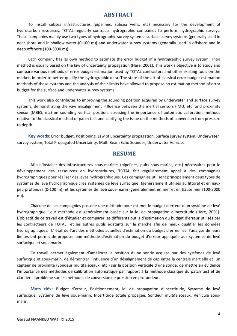
Classically, a surface survey system is composed of several sensors: a SVP probe, a GNSS positioning system
(GNSS receiver), a motion sensor (IMU5 /MRU6 and a gyro‐compass) and an acoustic sounder (Single or Multi‐
Beam Echo Sounder/MBES), all mounted on a vessel (see Figure 1 below). The MBES measures the depth of the
water. The SVP probe is used to determine the sound velocity profile (SVP) in the water column in order to
correct the depth measured by the MBES from sound speed variations. A sound velocity sensor (SVS) located
close to the MBES allows correcting the sound velocity close to transducer head. The motion sensor (IMU)
measures the attitude of the vessel (roll, pitch and yaw). The GNSS positioning system measures the vessel
position. The heave sensor is used to measure the vertical displacement of the vessel (heave). With most of
modern IMU, it is possible to measure both the attitude (roll, pitch and yaw) and the vertical displacement of
vessel (Ixblue, 2004).
Figure 1: Sensors and frames of a surface survey system (Bjørn & Einar, 2005)[modified]
Each sensor acquires its data in its own frame. The multiplicity of frames is a source of error. The various
frames of sensors (IMU frame and MBES frame) need to be aligned (Debese, 2013). As much as possible, sensors
alignment is achieved during the installation of the system. Possible misalignments between sensors are generally
corrected during the calibration phase (patch test) or after data acquisition (by automatic calibration methods
3Total Exploration & Production’s branch aims to discover and develop oil and gas fields to meet the world’s growing energy demand. 4These surveys identify any conditions at the seabed or in the foundation zone where hazardous subsurface features or unstable soil conditions exist. 5Inertial Measurement Unit 6Motion Reference Unit
7 Geraud NAANKEU WATI © 2015
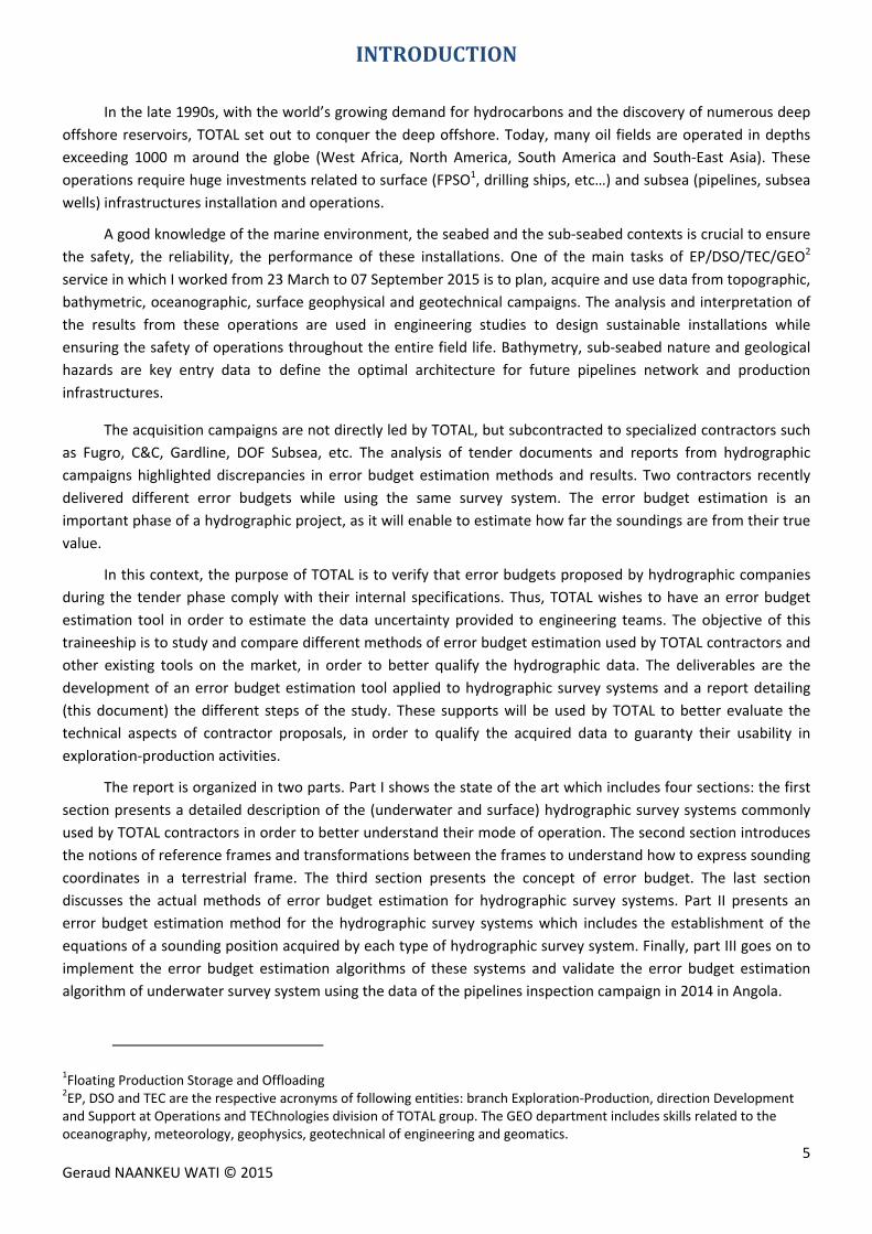
based on least squares). The Figure 2 below presents an example of misalignment between the MBES frame and
the IMU frame. More details about the manual calibration methods are further explained in the work of
(Skilltrade, 2012), (Debese, 2013) and (Seube, 2014). See (Seube, Levilly, & Keyetieu, 2015), for further
information about the automatic calibration methods.
Figure 2 Misalignment between MBES frame and IMU frame
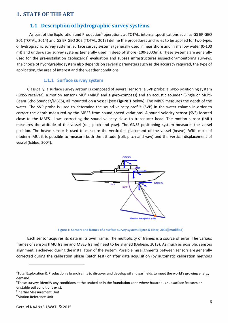
After the data acquisition phase, all the data of various sensors are loaded into data processing softwares.
The most used are CARIS, EIVA, HYSWEEP and QINSy. Data from the various sensors are not acquired exactly at
the same time (see Figure 3 below). Latency is introduced or can exist between sensors to take into account the
time of information transmission and the computation. It is commonly determined during the system calibration
phase because the data from different sensors needs to be synchronous during acquisition.
There are two main techniques to synchronize data. The first technique is to transfer the data on a single
system to date the time of receipt. To overcome transfer delays between the sensors, it is preferable to
synchronize the clocks of each sensor (second technique). The time stamp of data is then made at acquisition
time. Synchronization of various sensors is generally performed using a PPS signal (Pulse Per Second) from the
GNSS positioning system. For a detailed study on the synchronization methods, see the work of (Bjørn & Einar,
2005).
Figure 3: Illustration of asynchronous measurements in a surface survey system and Interpolation to MBES measurement time. (Bjørn & Einar, 2005)‐ [Modified]. The true measurement time is the time at which a data is measured. The time stamp is the time at which
8 Geraud NAANKEU WATI © 2015
1.1.2 Underwater survey system
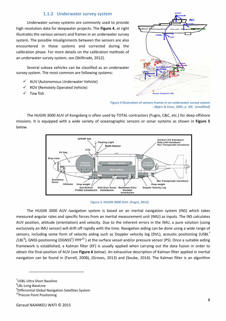
Underwater survey systems are commonly used to provide
high resolution data for deepwater projects. The Figure 4, at right
illustrates the various sensors and frames in an underwater survey
system. The possible misalignments between the sensors are also
encountered in these systems and corrected during the
calibration phase. For more details on the calibration methods of
an underwater survey system, see (Skilltrade, 2012).
Several subsea vehicles can be classified as an underwater survey system. The most common are following systems:
AUV (Autonomous Underwater Vehicle)
ROV (Remotely Operated Vehicle)
Tow fish
Figure 4 Illustration of sensors frames in an underwater survey system ‐ (Bjørn & Einar, 2005, p. 39) ‐ [modified]
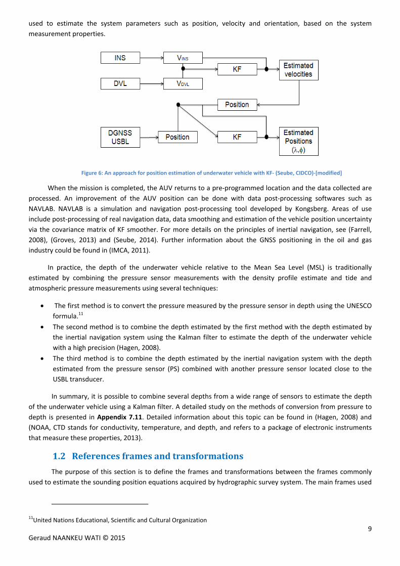
The HUGIN 3000 AUV of Kongsberg is often used by TOTAL contractors (Fugro, C&C, etc.) for deep offshore
missions. It is equipped with a wide variety of oceanographic sensors or sonar systems as shown in Figure 5
below.
Figure 5: HUGIN 3000 AUV‐ (Fugro, 2013)
The HUGIN 3000 AUV navigation system is based on an inertial navigation system (INS) which takes
measured angular rates and specific forces from an inertial measurement unit (IMU) as inputs. The INS calculates
AUV position, attitude (orientation) and velocity. Due to the inherent errors in the IMU, a pure solution (using
exclusively an IMU sensor) will drift off rapidly with the time. Navigation aiding can be done using a wide range of
sensors, including some form of velocity aiding such as Doppler velocity log (DVL), acoustic positioning (USBL7
/LBL8), GNSS positioning (DGNSS9/ PPP10 ) at the surface vessel and/or pressure sensor (PS). Once a suitable aiding
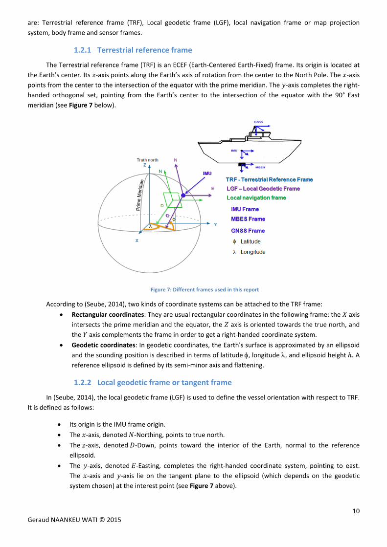
framework is established, a Kalman filter (KF) is usually applied when carrying out the data fusion in order to
obtain the final position of AUV (see Figure 6 below). An exhaustive description of Kalman filter applied in inertial
navigation can be found in (Farrell, 2008), (Groves, 2013) and (Seube, 2014). The Kalman filter is an algorithm
7USBL‐Ultra Short Baseline 8LBL‐Long BaseLine 9Differential Global Navigation Satellites System 10Precise Point Positioning
9 Geraud NAANKEU WATI © 2015
used to estimate the system parameters such as position, velocity and orientation, based on the system
measurement properties.
Figure 6: An approach for position estimation of underwater vehicle with KF‐ (Seube, CIDCO)‐[modified]
When the mission is completed, the AUV returns to a pre‐programmed location and the data collected are
processed. An improvement of the AUV position can be done with data post‐processing softwares such as
NAVLAB. NAVLAB is a simulation and navigation post‐processing tool developed by Kongsberg. Areas of use
include post‐processing of real navigation data, data smoothing and estimation of the vehicle position uncertainty
via the covariance matrix of KF smoother. For more details on the principles of inertial navigation, see (Farrell,
2008), (Groves, 2013) and (Seube, 2014). Further information about the GNSS positioning in the oil and gas
industry could be found in (IMCA, 2011).
In practice, the depth of the underwater vehicle relative to the Mean Sea Level (MSL) is traditionally
estimated by combining the pressure sensor measurements with the density profile estimate and tide and
atmospheric pressure measurements using several techniques:
The first method is to convert the pressure measured by the pressure sensor in depth using the UNESCO
formula.11
The second method is to combine the depth estimated by the first method with the depth estimated by
the inertial navigation system using the Kalman filter to estimate the depth of the underwater vehicle
with a high precision (Hagen, 2008).
The third method is to combine the depth estimated by the inertial navigation system with the depth
estimated from the pressure sensor (PS) combined with another pressure sensor located close to the
USBL transducer.
In summary, it is possible to combine several depths from a wide range of sensors to estimate the depth
of the underwater vehicle using a Kalman filter. A detailed study on the methods of conversion from pressure to
depth is presented in Appendix 7.11. Detailed information about this topic can be found in (Hagen, 2008) and
(NOAA, CTD stands for conductivity, temperature, and depth, and refers to a package of electronic instruments
that measure these properties, 2013).
1.2 Referencesframesandtransformations
The purpose of this section is to define the frames and transformations between the frames commonly
used to estimate the sounding position equations acquired by hydrographic survey system. The main frames used
11United Nations Educational, Scientific and Cultural Organization
10 Geraud NAANKEU WATI © 2015
are: Terrestrial reference frame (TRF), Local geodetic frame (LGF), local navigation frame or map projection
system, body frame and sensor frames.
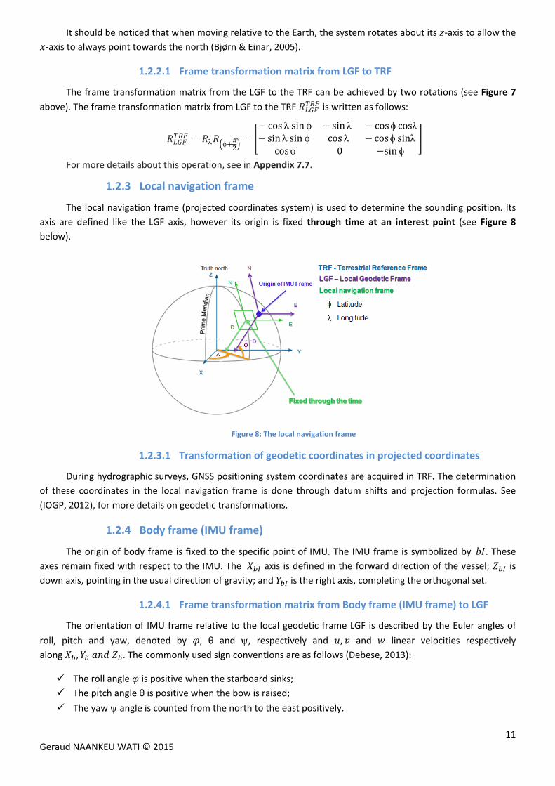
1.2.1 Terrestrial reference frame
The Terrestrial reference frame (TRF) is an ECEF (Earth‐Centered Earth‐Fixed) frame. Its origin is located at
the Earth’s center. Its ‐axis points along the Earth’s axis of rotation from the center to the North Pole. The ‐axis
points from the center to the intersection of the equator with the prime meridian. The ‐axis completes the right‐
handed orthogonal set, pointing from the Earth’s center to the intersection of the equator with the 90° East
meridian (see Figure 7 below).
Figure 7: Different frames used in this report
According to (Seube, 2014), two kinds of coordinate systems can be attached to the TRF frame:
Rectangular coordinates: They are usual rectangular coordinates in the following frame: the axis intersects the prime meridian and the equator, the axis is oriented towards the true north, and
the axis complements the frame in order to get a right‐handed coordinate system.
Geodetic coordinates: In geodetic coordinates, the Earth's surface is approximated by an ellipsoid
and the sounding position is described in terms of latitude, longitude, and ellipsoid height . A
reference ellipsoid is defined by itssemi‐minor axis and flattening.
1.2.2 Local geodetic frame or tangent frame
In (Seube, 2014), the local geodetic frame (LGF) is used to define the vessel orientation with respect to TRF.
It is defined as follows:
Its origin is the IMU frame origin.
The ‐axis, denoted ‐Northing, points to true north.
The ‐axis, denoted ‐Down, points toward the interior of the Earth, normal to the reference
ellipsoid.
The ‐axis, denoted ‐Easting, completes the right‐handed coordinate system, pointing to east.
The ‐axis and ‐axis lie on the tangent plane to the ellipsoid (which depends on the geodetic
system chosen) at the interest point (see Figure 7 above).
11 Geraud NAANKEU WATI © 2015
It should be noticed that when moving relative to the Earth, the system rotates about its ‐axis to allow the
‐axis to always point towards the north (Bjørn & Einar, 2005).
1.2.2.1 Frame transformation matrix from LGF to TRF
The frame transformation matrix from the LGF to the TRF can be achieved by two rotations (see Figure 7
above). The frame transformation matrix from LGF to the TRF is written as follows:
cos sin sin cos cossin sin cos cos sincos 0 sin
For more details about this operation, see in Appendix 7.7.
1.2.3 Local navigation frame
The local navigation frame (projected coordinates system) is used to determine the sounding position. Its
axis are defined like the LGF axis, however its origin is fixed through time at an interest point (see Figure 8
below).
Figure 8: The local navigation frame
1.2.3.1 Transformation of geodetic coordinates in projected coordinates
During hydrographic surveys, GNSS positioning system coordinates are acquired in TRF. The determination
of these coordinates in the local navigation frame is done through datum shifts and projection formulas. See
(IOGP, 2012), for more details on geodetic transformations.
1.2.4 Body frame (IMU frame)
The origin of body frame is fixed to the specific point of IMU. The IMU frame is symbolized by . These
axes remain fixed with respect to the IMU. The axis is defined in the forward direction of the vessel; is
down axis, pointing in the usual direction of gravity; and is the right axis, completing the orthogonal set.
1.2.4.1 Frame transformation matrix from Body frame (IMU frame) to LGF
The orientation of IMU frame relative to the local geodetic frame LGF is described by the Euler angles of
roll, pitch and yaw, denoted by , θ and , respectively and , and linear velocities respectively
along , . The commonly used sign conventions are as follows (Debese, 2013):
The roll angle is positive when the starboard sinks;
The pitch angle θ is positive when the bow is raised;
The yaw angle is counted from the north to the east positively.
12 Geraud NAANKEU WATI © 2015
According to (Seube, 2014), the frame transformation matrix from the IMU frame to the local geodetic
frame can be done through a series of three rotations. For more details about this series of rotations, see
Appendix 7.7.2.
The resulting transformation is:
φ, θ, ψ cosψcosθ cosψsinθsinφ sinψcosφ cosψsinθcosφ sinψsinφsinψcosθ sinψsinθsinφ cosψcosφ sinψsinθcosφ cosψsinφ
sinθ cosθsinφ cosθcosφ
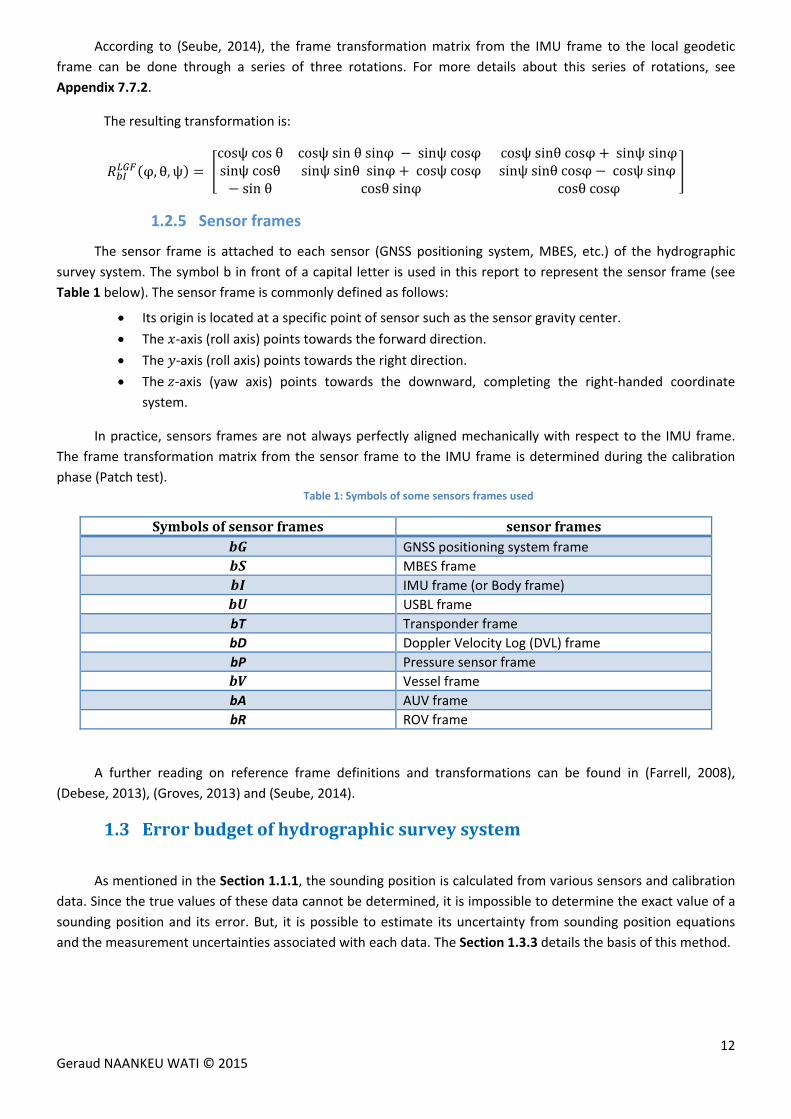
1.2.5 Sensor frames
The sensor frame is attached to each sensor (GNSS positioning system, MBES, etc.) of the hydrographic
survey system. The symbol b in front of a capital letter is used in this report to represent the sensor frame (see
Table 1 below). The sensor frame is commonly defined as follows:
Its origin is located at a specific point of sensor such as the sensor gravity center.
The ‐axis (roll axis) points towards the forward direction.
The ‐axis (roll axis) points towards the right direction.
The ‐axis (yaw axis) points towards the downward, completing the right‐handed coordinate
system.
In practice, sensors frames are not always perfectly aligned mechanically with respect to the IMU frame.
The frame transformation matrix from the sensor frame to the IMU frame is determined during the calibration
phase (Patch test). Table 1: Symbols of some sensors frames used
Symbolsofsensorframes sensorframes GNSS positioning system frame
MBES frame
IMU frame (or Body frame)
USBL frame
bT Transponder frame
bD Doppler Velocity Log (DVL) frame
bP Pressure sensor frame
Vessel frame
bA AUV frame
bR ROV frame
A further reading on reference frame definitions and transformations can be found in (Farrell, 2008),
(Debese, 2013), (Groves, 2013) and (Seube, 2014).
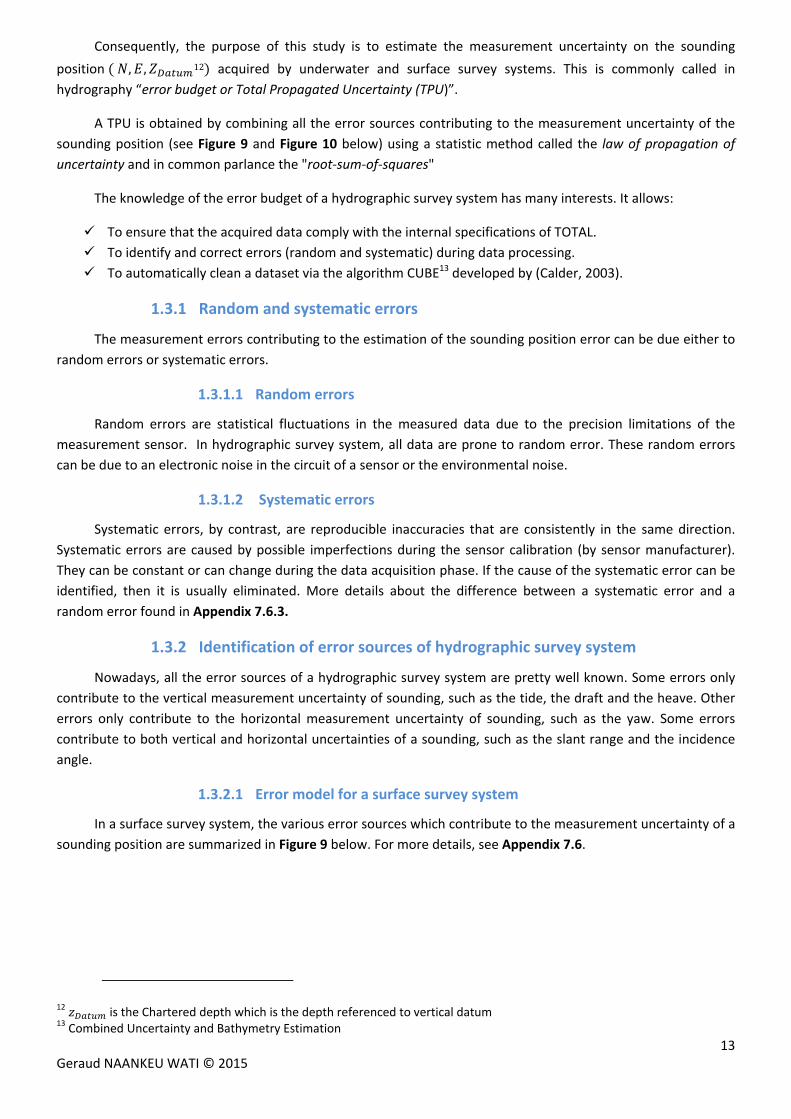
1.3 Errorbudgetofhydrographicsurveysystem
As mentioned in the Section 1.1.1, the sounding position is calculated from various sensors and calibration
data. Since the true values of these data cannot be determined, it is impossible to determine the exact value of a
sounding position and its error. But, it is possible to estimate its uncertainty from sounding position equations
and the measurement uncertainties associated with each data. The Section 1.3.3 details the basis of this method.
13 Geraud NAANKEU WATI © 2015
Consequently, the purpose of this study is to estimate the measurement uncertainty on the sounding
position , , 12 acquired by underwater and surface survey systems. This is commonly called in
hydrography “error budget or Total Propagated Uncertainty (TPU)”.
A TPU is obtained by combining all the error sources contributing to the measurement uncertainty of the
sounding position (see Figure 9 and Figure 10 below) using a statistic method called the law of propagation of
uncertainty and in common parlance the "root‐sum‐of‐squares"
The knowledge of the error budget of a hydrographic survey system has many interests. It allows:
To ensure that the acquired data comply with the internal specifications of TOTAL.
To identify and correct errors (random and systematic) during data processing.
To automatically clean a dataset via the algorithm CUBE13 developed by (Calder, 2003).
1.3.1 Random and systematic errors
The measurement errors contributing to the estimation of the sounding position error can be due either to
random errors or systematic errors.
1.3.1.1 Random errors
Random errors are statistical fluctuations in the measured data due to the precision limitations of the
measurement sensor. In hydrographic survey system, all data are prone to random error. These random errors
can be due to an electronic noise in the circuit of a sensor or the environmental noise.
1.3.1.2 Systematic errors
Systematic errors, by contrast, are reproducible inaccuracies that are consistently in the same direction.
Systematic errors are caused by possible imperfections during the sensor calibration (by sensor manufacturer).
They can be constant or can change during the data acquisition phase. If the cause of the systematic error can be
identified, then it is usually eliminated. More details about the difference between a systematic error and a
random error found in Appendix 7.6.3.
1.3.2 Identification of error sources of hydrographic survey system
Nowadays, all the error sources of a hydrographic survey system are pretty well known. Some errors only
contribute to the vertical measurement uncertainty of sounding, such as the tide, the draft and the heave. Other
errors only contribute to the horizontal measurement uncertainty of sounding, such as the yaw. Some errors
contribute to both vertical and horizontal uncertainties of a sounding, such as the slant range and the incidence
angle.
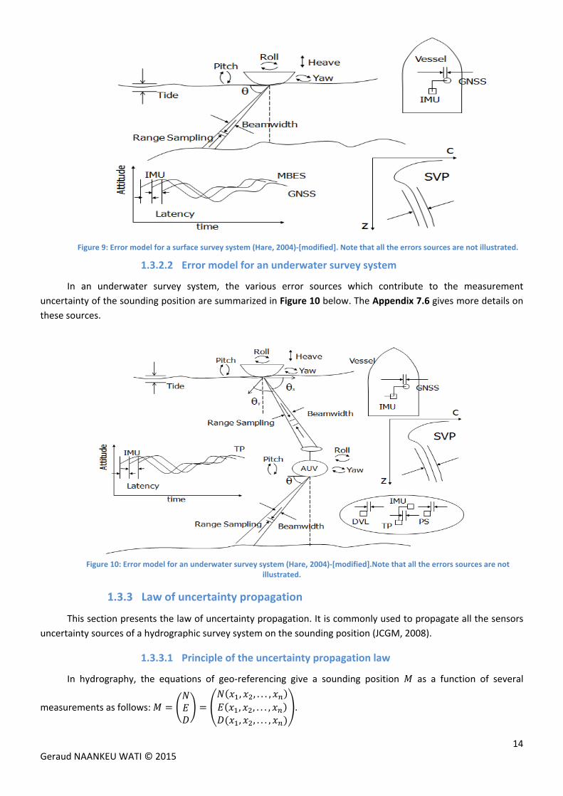
1.3.2.1 Error model for a surface survey system
In a surface survey system, the various error sources which contribute to the measurement uncertainty of a
sounding position are summarized in Figure 9 below. For more details, see Appendix 7.6.
12 is the Chartered depth which is the depth referenced to vertical datum 13 Combined Uncertainty and Bathymetry Estimation
14 Geraud NAANKEU WATI © 2015
Figure 9: Error model for a surface survey system (Hare, 2004)‐[modified]. Note that all the errors sources are not illustrated.
1.3.2.2 Error model for an underwater survey system
In an underwater survey system, the various error sources which contribute to the measurement
uncertainty of the sounding position are summarized in Figure 10 below. The Appendix 7.6 gives more details on
these sources.
Figure 10: Error model for an underwater survey system (Hare, 2004)‐[modified].Note that all the errors sources are not
illustrated.
1.3.3 Law of uncertainty propagation
This section presents the law of uncertainty propagation. It is commonly used to propagate all the sensors
uncertainty sources of a hydrographic survey system on the sounding position (JCGM, 2008).
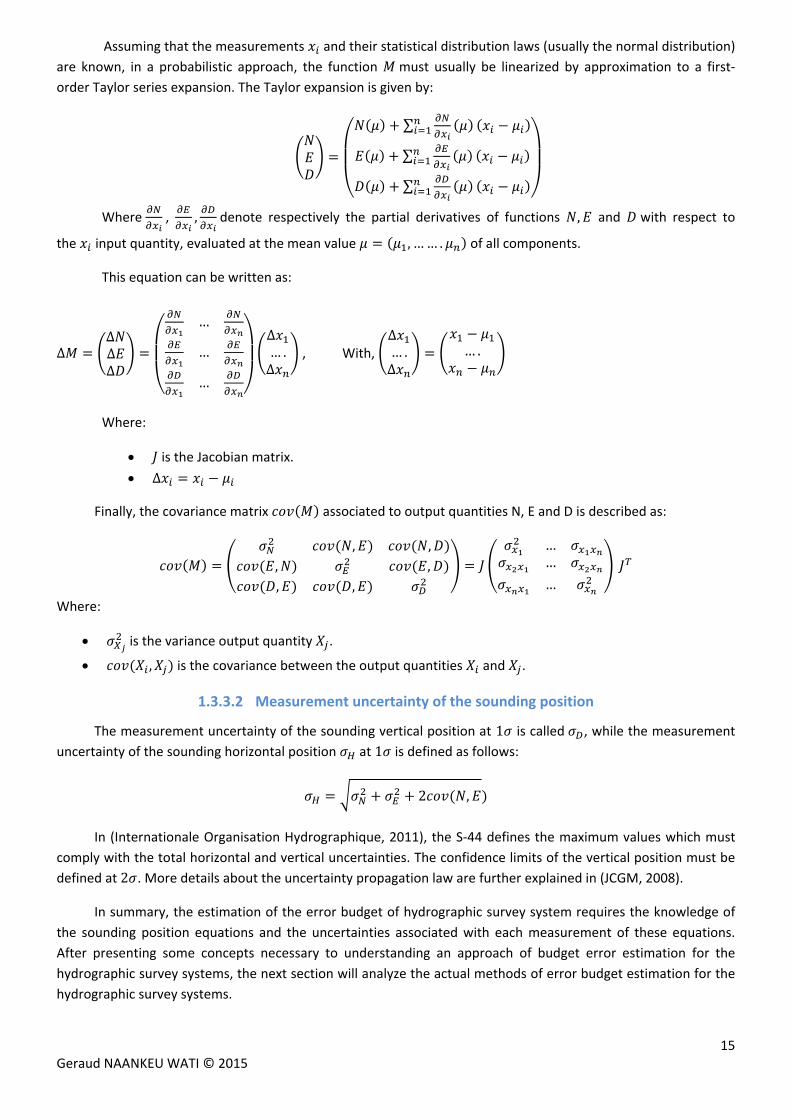
1.3.3.1 Principle of the uncertainty propagation law
In hydrography, the equations of geo‐referencing give a sounding position as a function of several
measurements as follows:, , . . . ,, , . . . ,, , . . . ,
.
15 Geraud NAANKEU WATI © 2015
Assuming that the measurements and their statistical distribution laws (usually the normal distribution)
are known, in a probabilistic approach, the function must usually be linearized by approximation to a first‐
order Taylor series expansion. The Taylor expansion is given by:
∑
∑
∑
Where , , denote respectively the partial derivatives of functions , and with respect to
the input quantity, evaluated at the mean value , …… . of all components.
This equation can be written as:
∆∆∆∆
…
…
…
∆… .∆
, With, ∆… .∆
… .
Where:
is the Jacobian matrix.
∆
Finally, the covariance matrix associated to output quantities N, E and D is described as:
, ,, ,, ,
……
…
Where:
is the variance output quantity .
, is the covariance between the output quantities and .
1.3.3.2 Measurement uncertainty of the sounding position
The measurement uncertainty of the sounding vertical position at 1 is called , while the measurement
uncertainty of the sounding horizontal position at 1 is defined as follows:
2 ,
In (Internationale Organisation Hydrographique, 2011), the S‐44 defines the maximum values which must
comply with the total horizontal and vertical uncertainties. The confidence limits of the vertical position must be
defined at2 . More details about the uncertainty propagation law are further explained in (JCGM, 2008).
In summary, the estimation of the error budget of hydrographic survey system requires the knowledge of
the sounding position equations and the uncertainties associated with each measurement of these equations.
After presenting some concepts necessary to understanding an approach of budget error estimation for the
hydrographic survey systems, the next section will analyze the actual methods of error budget estimation for the
hydrographic survey systems.
16 Geraud NAANKEU WATI © 2015
1.4 Analysisofactualmethodsoferrorbudgetestimationforhydrographicsurveysystems
At the end of the 20th century, the error budget estimation of a hydrographic survey system has been the
subject of several studies. Scientists like Erik Hammerstad (Hammerstad, 2001) and Rob Hare (Hare, 2001) have
proposed an estimation method for the error budget of a surface survey system. In 2005, a work group with
representatives from Statoil, Norwegian Hydrographic Service, Blom Maritime, Deep Ocean, Subsea 7 and
Geoconsult (Bjørn & Einar, 2005) has worked on the estimation of the sounding position offset due to the latency
effect between the sensors. The objective of their work was to derive well‐founded specifications on referencing
in hydrographic survey systems. In 2014, a group of researchers (Yanhui, Shuai, Shuxin, Zhiliang, & Hongwei,
2014) have analyzed the error budget of an underwater survey system.
But the most commonly used method in the industry for the error budget estimation of a surface survey
system was developed by Rob Hare in his technical report (Hare, 2001). It is implemented in various data
processing softwares such as CARIS, EIVA, HYSWEEP and QINSy and used by the TOTAL contractors (C&C, Fugro,
Gardline, etc.).The error budget estimation method of an underwater survey system can be used in a similar way
as surface survey system as mentioned in (Bjørn & Einar, 2005) and (Seube, 2014).
The objective of this section is to analyze Rob Hare’s approach and to identify the error sources classically
considered in the error budget estimation of underwater and surface survey systems. The results of this analysis
will be used in part II to propose an error budget estimation method for these systems. This analysis isn’t focused
on sensors error model estimation such as the model proposed by Xavier Lurton of IFREMER for the measurement
uncertainty estimation of MBES (Lurton, 2001). The popular methods of error sources estimation such as
(Hammerstad, 2001) and (Lurton, 2001) will be used in this study. Appendix 5.3 summarizes the methods of
estimation of measurement uncertainties of sensors in real time and post‐processing (Jason & Rob, 2011).
1.4.1 Analysis of the traditional method of the error budget estimation for
surface survey systems
In his technical report (Hare, 2001), Rob hare proposes a simplified method of error budget estimation for a
classical MBES surface survey. It consists in assessing separately the horizontal and vertical total uncertainties of
the sounding position as the square root of the sum of the variances of various uncertainty sources which
contribute to the sounding position. Nowadays, lots of hydrographic surveys are referenced relative to the
ellipsoid, commonly called ellipsoid referenced survey (ERS) (International Federation of Surveyors, 2006). The
position equations of a sounding acquired by the Ellipsoid referenced surveys will be also analyzed in this section.
1.4.1.1 Equations of sounding position for the surface survey systems
1.4.1.1.1 Classical hydrographic survey (Tide)
In the case of a classical MBES hydrographic survey, Rob Hare first expresses the horizontal position of a
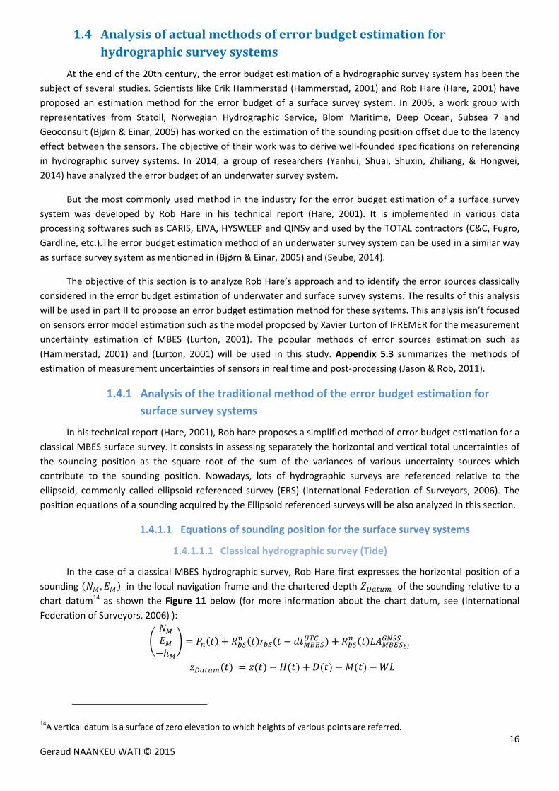
sounding , in the local navigation frame and the chartered depth of the sounding relative to a chart datum14 as shown the Figure 11 below (for more information about the chart datum, see (International
Federation of Surveyors, 2006) ):
14A vertical datum is a surface of zero elevation to which heights of various points are referred.
17 Geraud NAANKEU WATI © 2015
Figure 11 : Depth measurement corrections in the case of classical hydrographic survey ‐ (International Federation of Surveyors, 2006)‐[modified]
Where:
M is the sounding located at the seabed;
is the reference time from the GNSS positioning system in UTC;
, is the sounding horizontal position, resolved about the local navigation frame ;
is the latency between the GNSS positioning system and the MBES;
is the phase center position of GNSS positioning system, resolved about the axis of the local navigation
frame ;
is the rotation matrix from MBES frame to navigation frame ;
is the sounding position, resolved about the axis of MBES frame ;
is the lever arm offsets from the phase center position of GNSS positioning system and the
acoustic center of MBES (origin of MBES frame) , resolved about the axes of IMU frame;
is the dynamic draft;
is the measured heave (heave sensor);
is the measured or predicted tide;
is water height above chart datum (vertical datum);
is the ellipsoid height , which is the sounding height, resolved about the axis of the local navigation frame
is the vertical offset between the seabed and the IMU frame origin;
is the chartered depth.
1.4.1.1.2 Ellipsoid Reference Survey (ERS)
In the case of an ERS, the horizontal position equations of a sounding are similar to the classical
hydrographic survey. It requires the separation model (SEP) between the chart datum and the reference ellipsoid
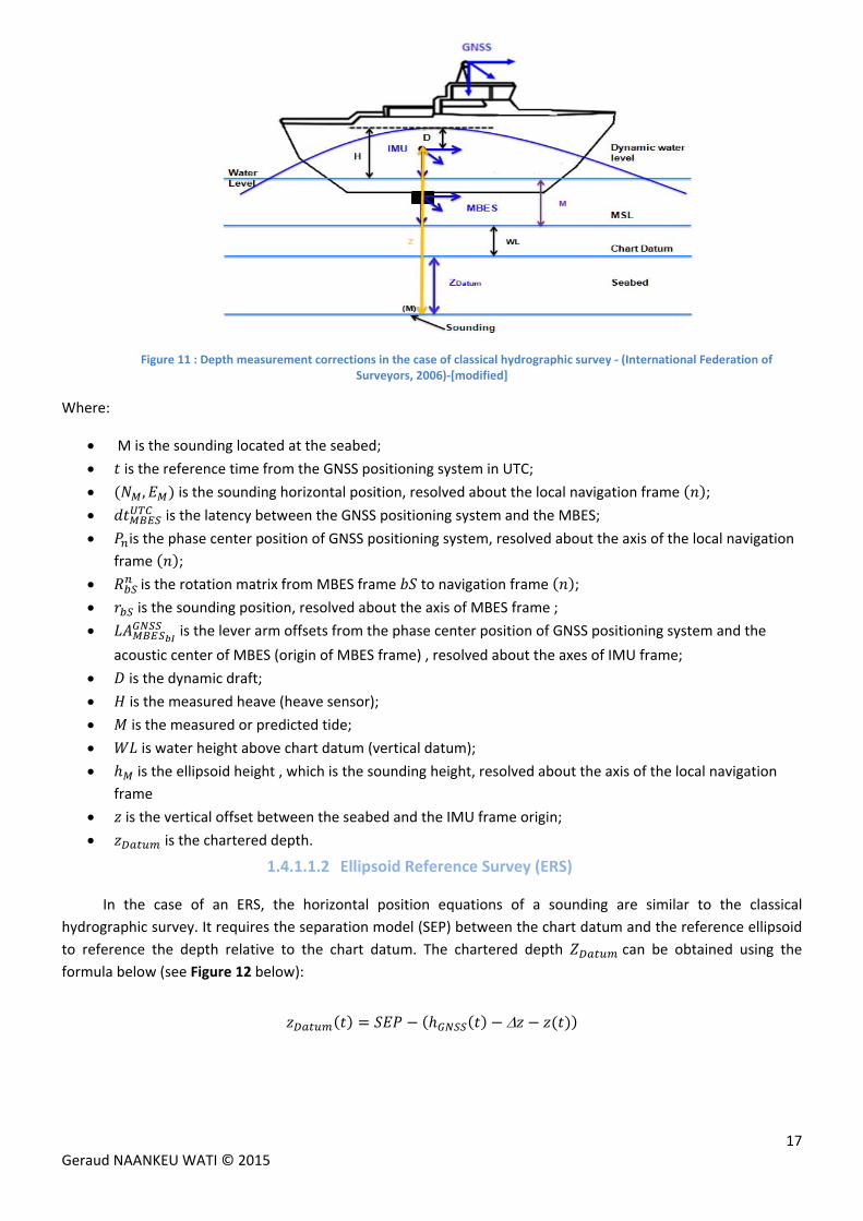
to reference the depth relative to the chart datum. The chartered depth can be obtained using the formula below (see Figure 12 below):
18 Geraud NAANKEU WATI © 2015
Figure 12: Depth measurement corrections in the case of GNSS survey‐ (International Federation of Surveyors, 2006)‐[modified]
Where:
is the separation model between the chart datum and the reference ellipsoid;
is the ellipsoid height of the GNSS positioning system;
is the vertical offset between the IMU and GNSS positioning system, resolved about the axis of the
local navigation frame;
is the vertical offset between the IMU and the GNSS positioning system, resolved about the axis of the
local navigation frame.
, the chartered depth.
1.4.1.2 Estimation of the error budget of surface survey system
In (Hare, 2001), the total horizontal and vertical uncertainties of the sounding position are estimated
separately by applying the law of uncertainty propagation on the equations of horizontal position and chartered
depth of a sounding, respectively. The assumptions made in Rob Hare’s method are:
1. All uncertainty sources are independent, unbiased and normally distributed.
2. The total uncertainty of the sounding horizontal position at 1 is equal to the square root of the sum
of variances of the horizontal uncertainties and by neglecting the covariance term . A
rigorous formulation of the total uncertainty of sounding horizontal position is defined as
2 (See in the Section 1.3.3).
3. The vertical position offset of a sounding due to the latency effect between the GNSS positioning system
and the MBES is negligible for the small pitch angles.
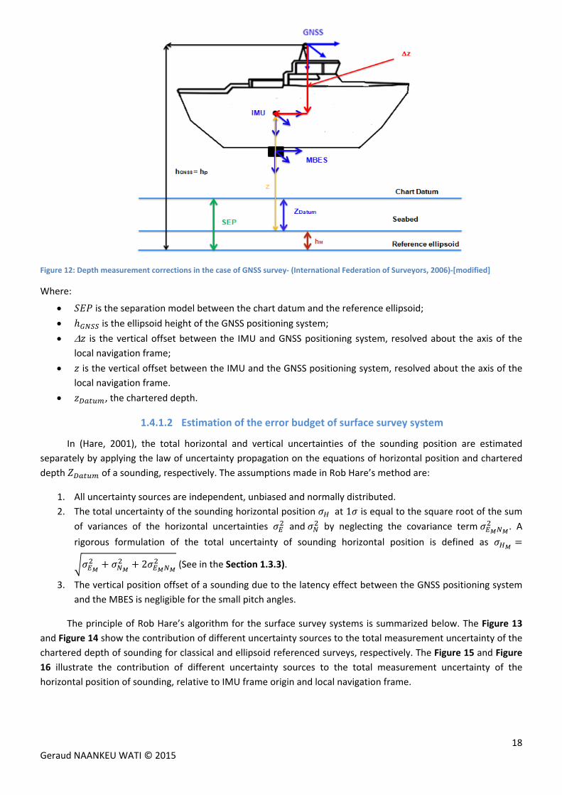
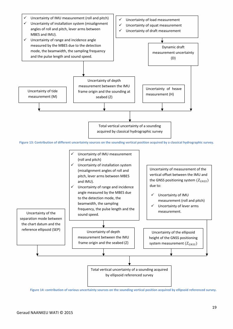
The principle of Rob Hare’s algorithm for the surface survey systems is summarized below. The Figure 13
and Figure 14 show the contribution of different uncertainty sources to the total measurement uncertainty of the
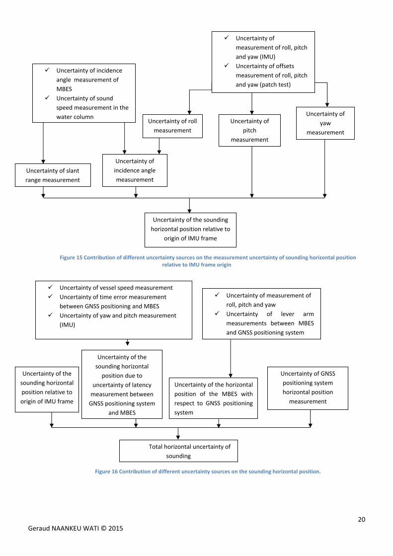
chartered depth of sounding for classical and ellipsoid referenced surveys, respectively. The Figure 15 and Figure
16 illustrate the contribution of different uncertainty sources to the total measurement uncertainty of the
horizontal position of sounding, relative to IMU frame origin and local navigation frame.
19 Geraud NAANKEU WATI © 2015
Figure 13: Contribution of different uncertainty sources on the sounding vertical position acquired by a classical hydrographic survey.
Figure 14: contribution of various uncertainty sources on the sounding vertical position acquired by ellipsoid referenced survey.
Uncertainty of depth
measurement between the IMU
frame origin and the seabed (Z)
Uncertainty of the
separation mode between
the chart datum and the
reference ellipsoid (SEP)
Total vertical uncertainty of a sounding acquired
by ellipsoid referenced survey
Uncertainty of IMU measurement
(roll and pitch)
Uncertainty of installation system
(misalignment angles of roll and
pitch, lever arms between MBES
and IMU).
Uncertainty of range and incidence
angle measured by the MBES due
to the detection mode, the
beamwidth, the sampling
frequency, the pulse length and the
sound speed.
Uncertainty of the ellipsoid
height of the GNSS positioning
system measurement
Uncertainty of measurement of the
vertical offset between the IMU and
the GNSS positioning system
due to:
Uncertainty of IMU
measurement (roll and pitch)
Uncertainty of lever arms
measurement.
Uncertainty of heave
measurement (H)
Dynamic draft
measurement uncertainty
(D)
Uncertainty of depth
measurement between the IMU
frame origin and the sounding at
seabed (Z)
Uncertainty of tide
measurement (M)
Total vertical uncertainty of a sounding
acquired by classical hydrographic survey
Uncertainty of load measurement
Uncertainty of squat measurement
Uncertainty of draft measurement
Uncertainty of IMU measurement (roll and pitch)
Uncertainty of installation system (misalignment
angles of roll and pitch, lever arms between
MBES and IMU).
Uncertainty of range and incidence angle
measured by the MBES due to the detection
mode, the beamwidth, the sampling frequency
and the pulse length and sound speed.
20 Geraud NAANKEU WATI © 2015
Figure 15 Contribution of different uncertainty sources on the measurement uncertainty of sounding horizontal position relative to IMU frame origin
Figure 16 Contribution of different uncertainty sources on the sounding horizontal position.
Uncertainty of incidence
angle measurement of
MBES
Uncertainty of sound
speed measurement in the
water column Uncertainty of roll
measurement
Uncertainty of
pitch
measurement
Uncertainty of
yaw
measurement
Uncertainty of
incidence angle
measurement
Uncertainty of slant
range measurement
Uncertainty of the sounding
horizontal position relative to
origin of IMU frame
Uncertainty of
measurement of roll, pitch
and yaw (IMU)
Uncertainty of offsets
measurement of roll, pitch
and yaw (patch test)
Uncertainty of measurement of
roll, pitch and yaw
Uncertainty of lever arm
measurements between MBES
and GNSS positioning system
Uncertainty of vessel speed measurement
Uncertainty of time error measurement
between GNSS positioning and MBES
Uncertainty of yaw and pitch measurement
(IMU)
Uncertainty of the
sounding horizontal
position relative to
origin of IMU frame
Uncertainty of the
sounding horizontal
position due to
uncertainty of latency
measurement between
GNSS positioning system
and MBES
Uncertainty of the horizontal
position of the MBES with
respect to GNSS positioning
system
Uncertainty of GNSS
positioning system
horizontal position
measurement
Total horizontal uncertainty of
sounding
21 Geraud NAANKEU WATI © 2015
1.4.2 Limitations of TPU classical estimation methods
The analysis of the estimation method of the error budget proposed by Rob Hare has allowed us to
highlight two important points:
The expression of the frame transformation matrix from the MBES Frame to local navigation frame ;
The position offset of a sounding due to the latency between the sensors.
1.4.2.1 Expression of the rotation matrix from the MBES Frame to the local
navigation frame
Below are the equations of sounding position resolved about the axis of local navigation frame defined by
Rob Hare’s approach:
With:
is the rotation matrix from MBES frame to local navigation frame ;
is the rotation matrix from IMU frame to local navigation frame ;
is the position of sounding M, resolved about the axis of MBES frame.
As mentioned in the Sections 1.1.1 and 1.2.4.1, the angles of roll , pitch and yaw, between the IMU
frame and the local geodetic frame, which is approximated at the local navigation frame (this approximation will
be explained later in part II) are measured by the IMU. While, the misalignment angles , , between the
MBES frame and the IMU frame are determined during the system calibration phase.
To determine the sounding position in the local navigation frame, Rob Hare expresses the rotation matrix
from MBES frame to local navigation frame as below:
, ,, , , , ,
With:
φ, θ, ψ cosψcosθ cosψsinθsinφ sinψcosφ cosψsinθcosφ sinψsinφsinψcosθ sinψsinθsinφ cosψcosφ sinψsinθcosφ cosψsinφ
sinθ cosθsinφ cosθcosφ
The measurement uncertainties of the corrected attitude angles , , after the system calibration
phase have been approximated as shown in Table 2 below:
Table 2: Measurement uncertainties of corrected attitude angles from (Hare, 2001)
To make this approximation, Rob Hare assumed that the measurement uncertainty of the sounding
horizontal position at 1 is equal to the square root of the sum of variances of the measurement
uncertainties of and , by neglecting the covariance term . In fact, all coupling terms between
measurement parameters are ignored for the sake of simplicity. However, they should be taking into account.
Corrected angles Measurement uncertainties of Corrected angles
22 Geraud NAANKEU WATI © 2015
From (Bjørn & Einar, 2005), (Hagen, 2006), (Farrell, 2008), (Groves, 2013), (Seube, 2014) and (Seube, Levilly,
& Keyetieu, 2015), the frame transformation matrix from MBES frame to local navigation frame results of
two successive rotations:
The frame transformation matrix between the MBES frame and the IMU frame and;
The frame transformation matrix between the IMU frame and the local navigation frame .
The resulting transformation is:
, ,, , , , , , ,
This approach is mostly used in the applications such as LIDAR (Gonçalves & Jalobeanu, 2011), mobile 3D
laser scanner and AUV.
According to (Farrell, 2008), (Groves, 2013 ) and (Seube, 2014), two successive rotations cannot be
expressed simply by adding the Euler angles ( , , # , , , , . Then,
the Rob Hare’s approach is not correct. The second approach is right and is more appropriate in hydrography to
determine the matrix rotation from the MBES frame to the local navigation frame. As in a hydrographic survey
system, the roll, pitch and yaw misalignments , , angles between the MBES frame and IMU frame are
determined during the system calibration phase. While, the roll, pitch and yaw angles , , between the IMU frame and local navigation frame are measured by the IMU during the acquisition phase.
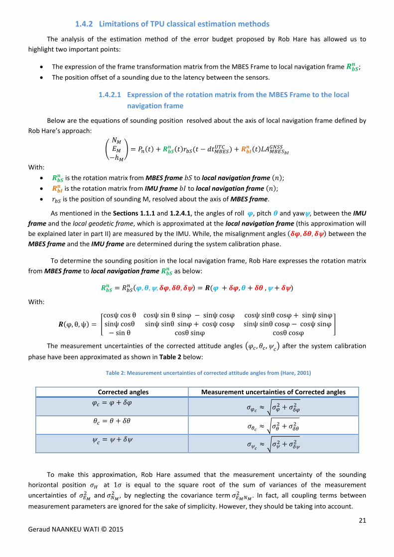
The Figure 17, Figure 18 and Figure 19 show the differences between the second approach and Rob hare’s
approach versus the depth, in easting, northing and depth, respectively. These differences are not null and vary
with the misalignment angles between the MBES frame and the IMU frame. Figure 19 below clearly presents that
a yaw misalignment affects the sounding vertical position. Other figures on the misalignments influence of
roll, pitch and yaw can be found in Appendix 7.5.
Figure 17: Influence of the misalignment yaw on ∆ with, °, °, °, ° . °.
0 50 100 150 200 250 300 350 400 450 500-0.08
-0.06
-0.04
-0.02
0
0.02
0.04
z (in m)
E
(in
m)
0°
0.1°
0.3°
0.7°
1°
23 Geraud NAANKEU WATI © 2015
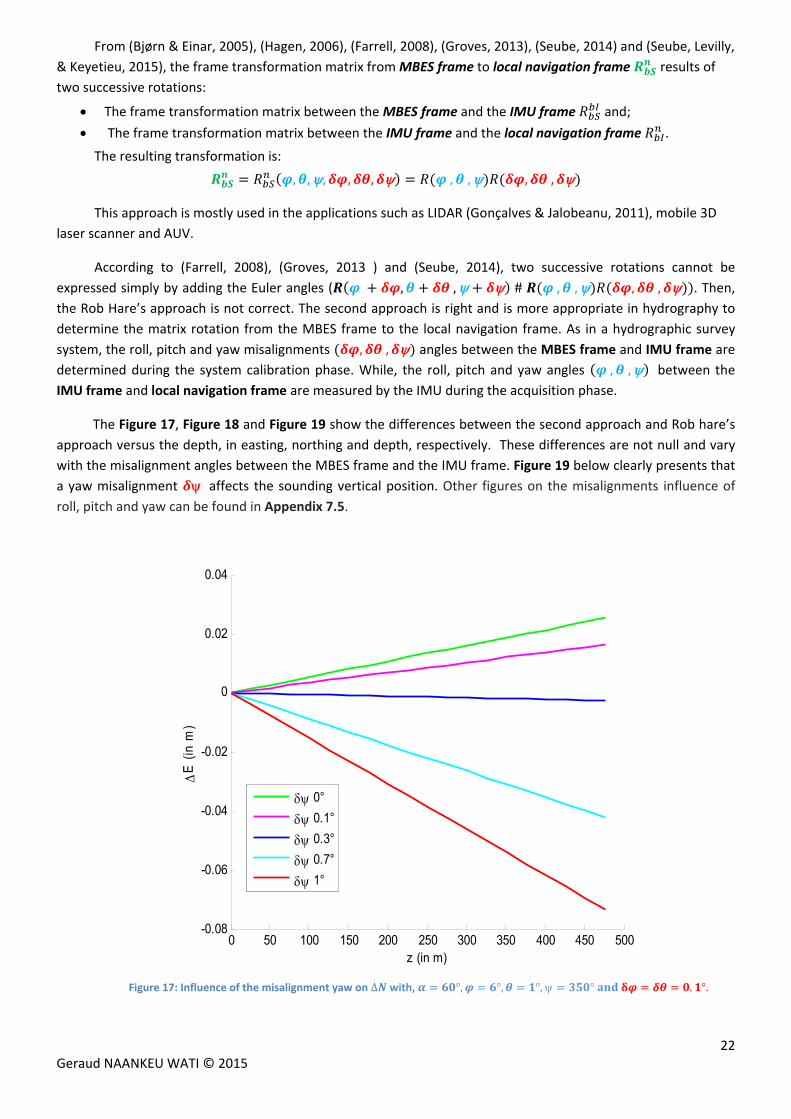
Figure 18: Influence of the misalignment yaw on ∆ with, °, °, °, ° . °.
Figure 19 : Influence of the misalignment yaw on ∆ with, °, °, °, ° . °.
The misalignment angles between the MBES frame and IMU frame are not always small (like 0.1° shown in
the figures above) in the hydrographic survey systems used by TOTAL contractors (see Table 3 below). This could
lead to significant offset on the sounding position.
0 50 100 150 200 250 300 350 400 450 500-1.4
-1.2
-1
-0.8
-0.6
-0.4
-0.2
0
z (in m)
N
(in m
)
0°
0.1°
0.3°
0.7°
1°
0 50 100 150 200 250 300 350 400 450 5000
0.05
0.1
0.15
0.2
0.25
0.3
0.35
0.4
z (in m)
h
(in m
)
0°
0.1°
0.3°
0.7°
1°
24 Geraud NAANKEU WATI © 2015
Table 3: Calibration using the patch Test on the vessel Fugro IMPI ‐Cap Lopez 2012
Startingofproject 15/12/2012 Endofproject17/12/2012Rollmisalignment 2.35 ° 2.05°
Pitchmisalignment ‐1° ‐1°
Yawmisalignment ‐1.0° ‐1.10°
LatencyMBES/GNSS 0.38 s ‐0.15 s
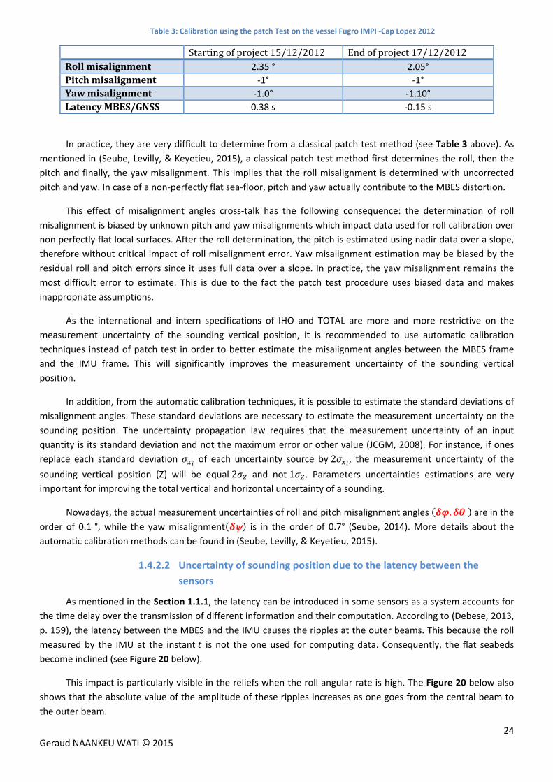
In practice, they are very difficult to determine from a classical patch test method (see Table 3 above). As
mentioned in (Seube, Levilly, & Keyetieu, 2015), a classical patch test method first determines the roll, then the
pitch and finally, the yaw misalignment. This implies that the roll misalignment is determined with uncorrected
pitch and yaw. In case of a non‐perfectly flat sea‐floor, pitch and yaw actually contribute to the MBES distortion.
This effect of misalignment angles cross‐talk has the following consequence: the determination of roll
misalignment is biased by unknown pitch and yaw misalignments which impact data used for roll calibration over
non perfectly flat local surfaces. After the roll determination, the pitch is estimated using nadir data over a slope,
therefore without critical impact of roll misalignment error. Yaw misalignment estimation may be biased by the
residual roll and pitch errors since it uses full data over a slope. In practice, the yaw misalignment remains the
most difficult error to estimate. This is due to the fact the patch test procedure uses biased data and makes
inappropriate assumptions.
As the international and intern specifications of IHO and TOTAL are more and more restrictive on the
measurement uncertainty of the sounding vertical position, it is recommended to use automatic calibration
techniques instead of patch test in order to better estimate the misalignment angles between the MBES frame
and the IMU frame. This will significantly improves the measurement uncertainty of the sounding vertical
position.
In addition, from the automatic calibration techniques, it is possible to estimate the standard deviations of
misalignment angles. These standard deviations are necessary to estimate the measurement uncertainty on the
sounding position. The uncertainty propagation law requires that the measurement uncertainty of an input
quantity is its standard deviation and not the maximum error or other value (JCGM, 2008). For instance, if ones
replace each standard deviation of each uncertainty source by2 , the measurement uncertainty of the
sounding vertical position (Z) will be equal2 and not1 . Parameters uncertainties estimations are very
important for improving the total vertical and horizontal uncertainty of a sounding.
Nowadays, the actual measurement uncertainties of roll and pitch misalignment angles , are in the order of 0.1 °, while the yaw misalignment is in the order of 0.7° (Seube, 2014). More details about the
automatic calibration methods can be found in (Seube, Levilly, & Keyetieu, 2015).
1.4.2.2 Uncertainty of sounding position due to the latency between the
sensors
As mentioned in the Section 1.1.1, the latency can be introduced in some sensors as a system accounts for
the time delay over the transmission of different information and their computation. According to (Debese, 2013,
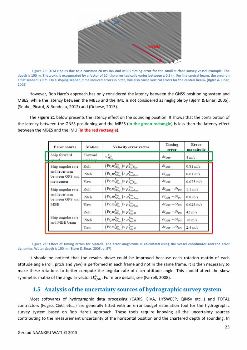
p. 159), the latency between the MBES and the IMU causes the ripples at the outer beams. This because the roll
measured by the IMU at the instant is not the one used for computing data. Consequently, the flat seabeds
become inclined (see Figure 20 below).
This impact is particularly visible in the reliefs when the roll angular rate is high. The Figure 20 below also
shows that the absolute value of the amplitude of these ripples increases as one goes from the central beam to
the outer beam.
25 Geraud NAANKEU WATI © 2015
Figure 20: DTM ripples due to a constant 20 ms INS and MBES timing error for the small surface survey vessel example. The depth is 100 m. The z‐axis is exaggerated by a factor of 10; the error typically varies between ± 0.5 m. For the central beam, the error on a flat seabed is 0 m. On a sloping seabed, time induced errors in pitch, will also cause vertical errors for the central beam‐ (Bjørn & Einar, 2005)
However, Rob Hare’s approach has only considered the latency between the GNSS positioning system and
MBES, while the latency between the MBES and the IMU is not considered as negligible by (Bjørn & Einar, 2005),
(Seube, Picard, & Rondeau, 2012) and (Debese, 2013).
The Figure 21 below presents the latency effect on the sounding position. It shows that the contribution of
the latency between the GNSS positioning and the MBES (in the green rectangle) is less than the latency effect
between the MBES and the IMU (in the red rectangle).
Figure 21: Effect of timing errors for Sjøtroll. The error magnitude is calculated using the vessel coordinates and the error dynamics. Water depth is 100 m. (Bjørn & Einar, 2005, p. 97)
It should be noticed that the results above could be improved because each rotation matrix of each
attitude angle (roll, pitch and yaw) is performed in each frame and not in the same frame. It is then necessary to
make these rotations to better compute the angular rate of each attitude angle. This should affect the skew
symmetric matrix of the angular vectorΩ / . For more details, see (Farrell, 2008).
1.5 Analysisoftheuncertaintysourcesofhydrographicsurveysystem
Most softwares of hydrographic data processing (CARIS, EIVA, HYSWEEP, QINSy etc…) and TOTAL
contractors (Fugro, C&C, etc…) are generally fitted with an error budget estimation tool for the hydrographic
survey system based on Rob Hare’s approach. These tools require knowing all the uncertainty sources
contributing to the measurement uncertainty of the horizontal position and the chartered depth of sounding. In
26 Geraud NAANKEU WATI © 2015
practice, some uncertainty sources are neglected. Analyzing the different softwares on the market, this part tries
to determine whether some uncertainties could be neglected or not.
1.5.1 Analysis of the uncertainty sources of a surface survey system
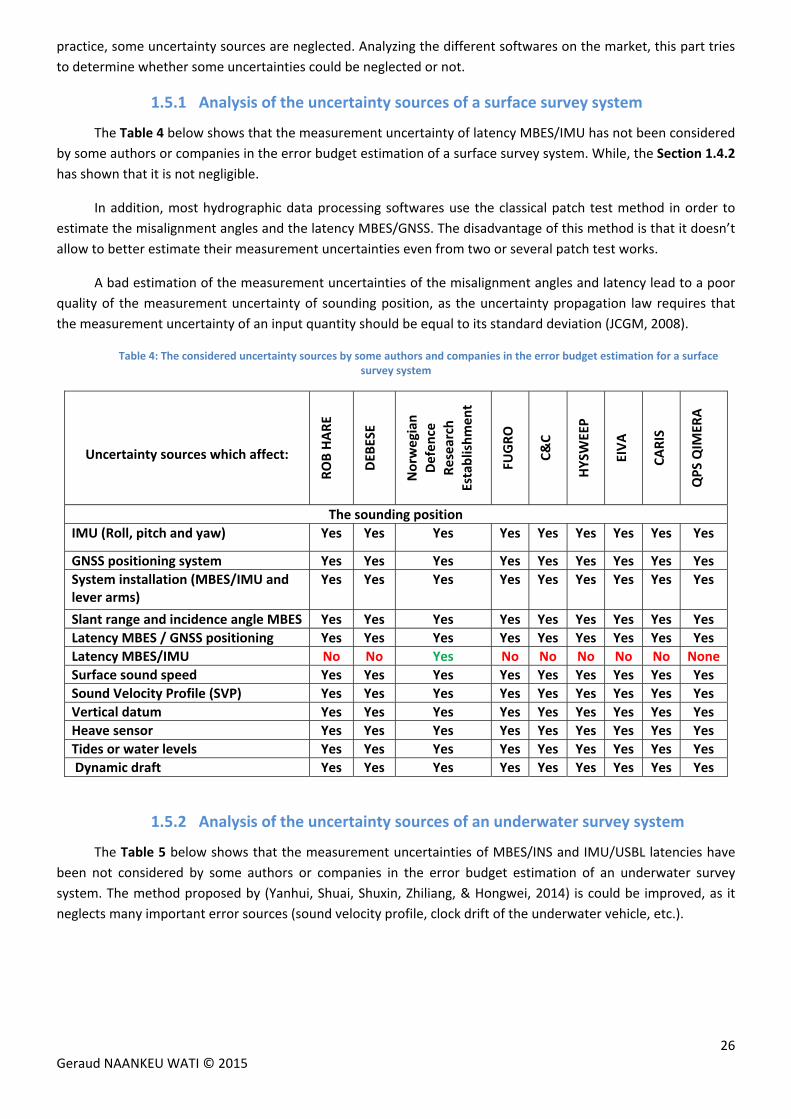
The Table 4 below shows that the measurement uncertainty of latency MBES/IMU has not been considered
by some authors or companies in the error budget estimation of a surface survey system. While, the Section 1.4.2
has shown that it is not negligible.
In addition, most hydrographic data processing softwares use the classical patch test method in order to
estimate the misalignment angles and the latency MBES/GNSS. The disadvantage of this method is that it doesn’t
allow to better estimate their measurement uncertainties even from two or several patch test works.
A bad estimation of the measurement uncertainties of the misalignment angles and latency lead to a poor
quality of the measurement uncertainty of sounding position, as the uncertainty propagation law requires that
the measurement uncertainty of an input quantity should be equal to its standard deviation (JCGM, 2008).
Table 4: The considered uncertainty sources by some authors and companies in the error budget estimation for a surface survey system
Uncertainty sources which affect:
ROB HARE
DEB
ESE
Norw
egian
Defence
Research
Establishment
FUGRO
C&C
HYSW
EEP
EIVA
CARIS
QPS QIM
ERA
The sounding position
IMU (Roll, pitch and yaw) Yes Yes Yes Yes Yes Yes Yes Yes Yes
GNSS positioning system Yes Yes Yes Yes Yes Yes Yes Yes Yes
System installation (MBES/IMU and lever arms)
Yes Yes Yes Yes Yes Yes Yes Yes Yes
Slant range and incidence angle MBES Yes Yes Yes Yes Yes Yes Yes Yes Yes
Latency MBES / GNSS positioning Yes Yes Yes Yes Yes Yes Yes Yes Yes
Latency MBES/IMU No No Yes No No No No No None
Surface sound speed Yes Yes Yes Yes Yes Yes Yes Yes Yes
Sound Velocity Profile (SVP) Yes Yes Yes Yes Yes Yes Yes Yes Yes
Vertical datum Yes Yes Yes Yes Yes Yes Yes Yes Yes
Heave sensor Yes Yes Yes Yes Yes Yes Yes Yes Yes
Tides or water levels Yes Yes Yes Yes Yes Yes Yes Yes Yes
Dynamic draft Yes Yes Yes Yes Yes Yes Yes Yes Yes
1.5.2 Analysis of the uncertainty sources of an underwater survey system
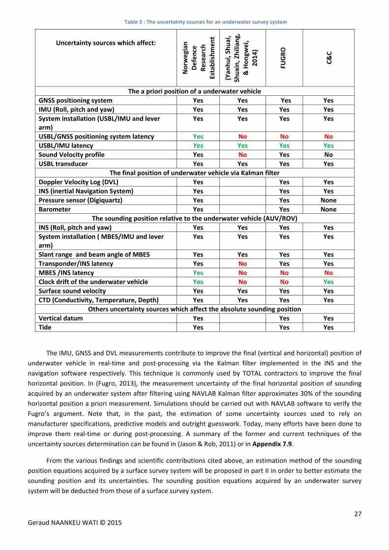
The Table 5 below shows that the measurement uncertainties of MBES/INS and IMU/USBL latencies have
been not considered by some authors or companies in the error budget estimation of an underwater survey
system. The method proposed by (Yanhui, Shuai, Shuxin, Zhiliang, & Hongwei, 2014) is could be improved, as it
neglects many important error sources (sound velocity profile, clock drift of the underwater vehicle, etc.).
27 Geraud NAANKEU WATI © 2015
Table 5 : The uncertainty sources for an underwater survey system
The IMU, GNSS and DVL measurements contribute to improve the final (vertical and horizontal) position of
underwater vehicle in real‐time and post‐processing via the Kalman filter implemented in the INS and the
navigation software respectively. This technique is commonly used by TOTAL contractors to improve the final
horizontal position. In (Fugro, 2013), the measurement uncertainty of the final horizontal position of sounding
acquired by an underwater system after filtering using NAVLAB Kalman filter approximates 30% of the sounding
horizontal position a priori measurement. Simulations should be carried out with NAVLAB software to verify the
Fugro’s argument. Note that, in the past, the estimation of some uncertainty sources used to rely on
manufacturer specifications, predictive models and outright guesswork. Today, many efforts have been done to
improve them real‐time or during post‐processing. A summary of the former and current techniques of the
uncertainty sources determination can be found in (Jason & Rob, 2011) or in Appendix 7.9.
From the various findings and scientific contributions cited above, an estimation method of the sounding
position equations acquired by a surface survey system will be proposed in part II in order to better estimate the
sounding position and its uncertainties. The sounding position equations acquired by an underwater survey
system will be deducted from those of a surface survey system.
Uncertainty sources which affect:
Norw
egian
Defence
Research
Establishment
(Yan
hui, Shuai,
Shuxin, Zhilian
g,
& Hongw
ei,
2014)
FUGRO
C&C
The a priori position of a underwater vehicle
GNSS positioning system Yes Yes Yes Yes
IMU (Roll, pitch and yaw) Yes Yes Yes Yes
System installation (USBL/IMU and lever arm)
Yes Yes Yes Yes
USBL/GNSS positioning system latency Yes No No No
USBL/IMU latency Yes Yes Yes Yes
Sound Velocity profile Yes No Yes No
USBL transducer Yes Yes Yes Yes
The final position of underwater vehicle via Kalman filter
Doppler Velocity Log (DVL) Yes Yes Yes
INS (inertial Navigation System) Yes Yes Yes
Pressure sensor (Digiquartz) Yes Yes None
Barometer Yes Yes None
The sounding position relative to the underwater vehicle (AUV/ROV)
INS (Roll, pitch and yaw) Yes Yes Yes Yes
System installation ( MBES/IMU and lever arm)
Yes Yes Yes Yes
Slant range and beam angle of MBES Yes Yes Yes Yes
Transponder/INS latency Yes No Yes Yes
MBES /INS latency Yes No No No
Clock drift of the underwater vehicle Yes No No Yes
Surface sound velocity Yes Yes Yes Yes
CTD (Conductivity, Temperature, Depth) Yes Yes Yes Yes
Others uncertainty sources which affect the absolute sounding position
Vertical datum Yes Yes Yes
Tide Yes Yes Yes
28 Geraud NAANKEU WATI © 2015
2. PROPOSEDMETHODFORERRORBUDGETESTIMATIONFORHYDROGRAPHICSURVEYSYSTEMS
The purpose of this second part is to present a simplified method of error budget estimation for surface
and underwater survey systems. The equations of sounding position acquired by these systems will be established
in order to estimate the error budget for each type of hydrographic survey system using the law of uncertainty
propagation (see Section1.3.3).
2.1 Equationsofsoundingpositionofasurfacesurveysystem
2.1.1 Geometric description of a surface multi beam survey system
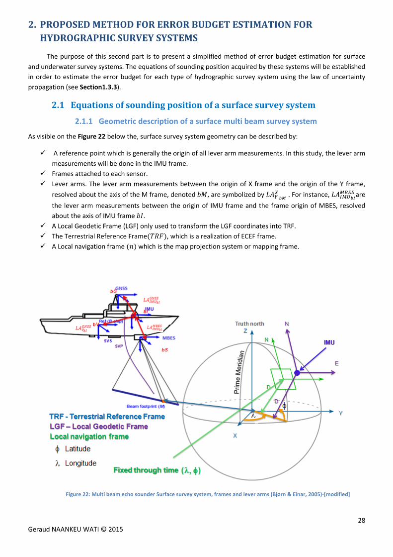
As visible on the Figure 22 below the, surface survey system geometry can be described by:
A reference point which is generally the origin of all lever arm measurements. In this study, the lever arm
measurements will be done in the IMU frame.
Frames attached to each sensor.
Lever arms. The lever arm measurements between the origin of X frame and the origin of the Y frame,
resolved about the axis of the M frame, denoted , are symbolized by . For instance, are
the lever arm measurements between the origin of IMU frame and the frame origin of MBES, resolved
about the axis of IMU frame .
A Local Geodetic Frame (LGF) only used to transform the LGF coordinates into TRF.
The Terrestrial Reference Frame , which is a realization of ECEF frame.
A Local navigation frame which is the map projection system or mapping frame.
Figure 22: Multi beam echo sounder Surface survey system, frames and lever arms (Bjørn & Einar, 2005)‐[modified]
29 Geraud NAANKEU WATI © 2015
2.1.2 Geo‐referencing equations in the navigation frame
The purpose of this section is to determine the equations of a sounding position acquired by a surface
survey system in the local navigation frame. This work will establish equations of a sounding position , first in the
MBES frame, then in the IMU frame, the terrestrial reference frame (TRF) and finally in the local navigation frame
or map projection frame.
In this report, the position equations of a sounding will be expressed in the mapping frame coordinate
system. These position equations will then be derived using the symbolic language tool of Maxima or Matlab in
order to determine the uncertainty on the sounding position. The approach hypotheses are:
1. The lever arms offsets are already known and resolved about the axis of IMU frame.
2. The misalignments angles between the MBES frame and the IMU frame exist and are known.
3. The sound speed profile of the water column is adequately known.
4. The data acquired by the different sensors of the survey system are synchronous. That is to say that all
the sensors measurements are acquired at the same time. But, it is not always the case because there is
generally latency between the sensors. The position offset a sounding due to the latency will be
determined later.
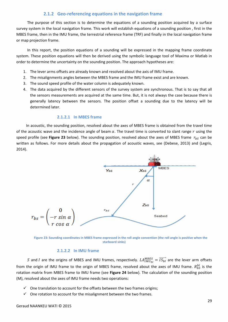
2.1.2.1 In MBES frame
In acoustic, the sounding position, resolved about the axes of MBES frame is obtained from the travel time
of the acoustic wave and the incidence angle of beam . The travel time is converted to slant range using the
speed profile (see Figure 23 below). The sounding position, resolved about the axes of MBES frame can be
written as follows. For more details about the propagation of acoustic waves, see (Debese, 2013) and (Legris,
2014).
Figure 23: Sounding coordinates in MBES frame expressed in the roll angle convention (the roll angle is positive when the starboard sinks)
2.1.2.2 In IMU frame
and are the origins of MBES and IMU frames, respectively. are the lever arm offsets
from the origin of IMU frame to the origin of MBES frame, resolved about the axes of IMU frame. is the
rotation matrix from MBES frame to IMU frame (see Figure 24 below). The calculation of the sounding position
(M), resolved about the axes of IMU frame needs two operations:
One translation to account for the offsets between the two frames origins;
One rotation to account for the misalignment between the two frames.
30 Geraud NAANKEU WATI © 2015
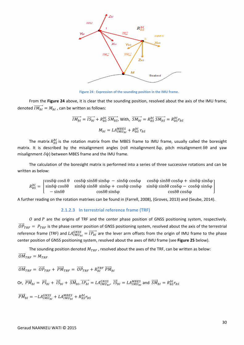
Figure 24 : Expression of the sounding position in the IMU frame.
From the Figure 24 above, it is clear that the sounding position, resolved about the axis of the IMU frame,
denoted , can be written as follows:
, With,
The matrix is the rotation matrix from the MBES frame to IMU frame, usually called the boresight
matrix. It is described by the misalignment angles (roll misalignmentδφ, pitch misalignmentδθ and yaw misalignment ψ) between MBES frame and the IMU frame.
The calculation of the boresight matrix is performed into a series of three successive rotations and can be
written as below:
cosδψcosδθ cosδψsinδθsinδφ sinδψcosδφ cosδψsinδθcosδφ sinδψsinδφsinδψcosδθ sinδψsinδθsinδφ cosδψcosδφ sinδψsinδθcosδφ cosδψsinδφ
sinδθ cosδθsinδφ cosδθcosδφ
A further reading on the rotation matrixes can be found in (Farrell, 2008), (Groves, 2013) and (Seube, 2014).
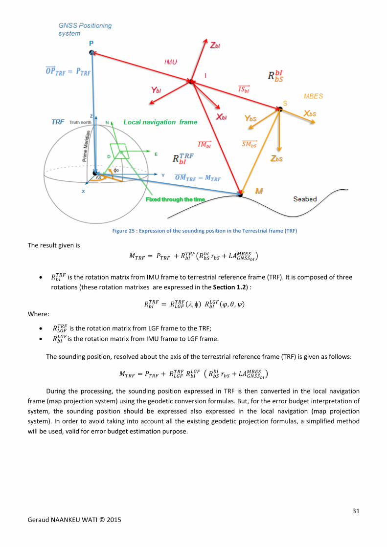
2.1.2.3 In terrestrial reference frame (TRF)
and are the origins of TRF and the center phase position of GNSS positioning system, respectively.
is the phase center position of GNSS positioning system, resolved about the axis of the terrestrial
reference frame (TRF) and are the lever arm offsets from the origin of IMU frame to the phase
center position of GNSS positioning system, resolved about the axes of IMU frame (see Figure 25 below).
The sounding position denoted , resolved about the axes of the TRF, can be written as below:
Or, , , and
31 Geraud NAANKEU WATI © 2015
Figure 25 : Expression of the sounding position in the Terrestrial frame (TRF)
The result given is
is the rotation matrix from IMU frame to terrestrial reference frame (TRF). It is composed of three
rotations (these rotation matrixes are expressed in the Section 1.2) :
, , ,
Where:
is the rotation matrix from LGF frame to the TRF;
is the rotation matrix from IMU frame to LGF frame.
The sounding position, resolved about the axis of the terrestrial reference frame (TRF) is given as follows:
During the processing, the sounding position expressed in TRF is then converted in the local navigation
frame (map projection system) using the geodetic conversion formulas. But, for the error budget interpretation of
system, the sounding position should be expressed also expressed in the local navigation (map projection
system). In order to avoid taking into account all the existing geodetic projection formulas, a simplified method
will be used, valid for error budget estimation purpose.
32 Geraud NAANKEU WATI © 2015
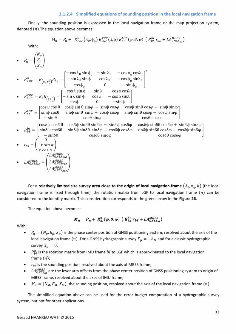
2.1.2.4 Simplified equations of sounding position in the local navigation frame
Finally, the sounding position is expressed in the local navigation frame or the map projection system,
denoted .The equation above becomes:
, , , ,
With:
cos sin sin cos cossin sin cos cos sin cos 0 sin
cos sin sin cos cossin sin cos cos sincos 0 sin
cosψcosθ cosψsinθsinφ sinψcosφ cosψsinθcosφ sinψsinφsinψcosθ sinψsinθsinφ cosψcosφ sinψsinθcosφ cosψsinφ
sinθ cosθsinφ cosθcosφ
cosδψcosδθ cosδψsinδθsinδφ sinδψcosδφ cosδψsinδθcosδφ sinδψsinδφsinδψcosδθ sinδψsinδθsinδφ cosδψcosδφ sinδψsinδθcosδφ cosδψsinδφ
sinδθ cosδθsinδφ cosδθcosδφ
0
For a relatively limited size survey area close to the origin of local navigation frame , , (the local
navigation frame is fixed through time), the rotation matrix from LGF to local navigation frame can be
considered to the identity matrix. This consideration corresponds to the green arrow in the Figure 26.
The equation above becomes:
, ,
With:
, , is the phase center position of GNSS positioning system, resolved about the axis of the
local navigation frame . For a GNSS hydrographic survey and for a classic hydrographic
survey 0.
is the rotation matrix from IMU frame to LGF which is approximated to the local navigation
frame ;
is the sounding position, resolved about the axis of MBES frame;
are the lever arm offsets from the phase center position of GNSS positioning system to origin of
MBES frame, resolved about the axes of IMU frame;
, , , the sounding position, resolved about the axis of the local navigation frame .
The simplified equation above can be used for the error budget computation of a hydrographic survey
system, but not for other applications.
33 Geraud NAANKEU WATI © 2015
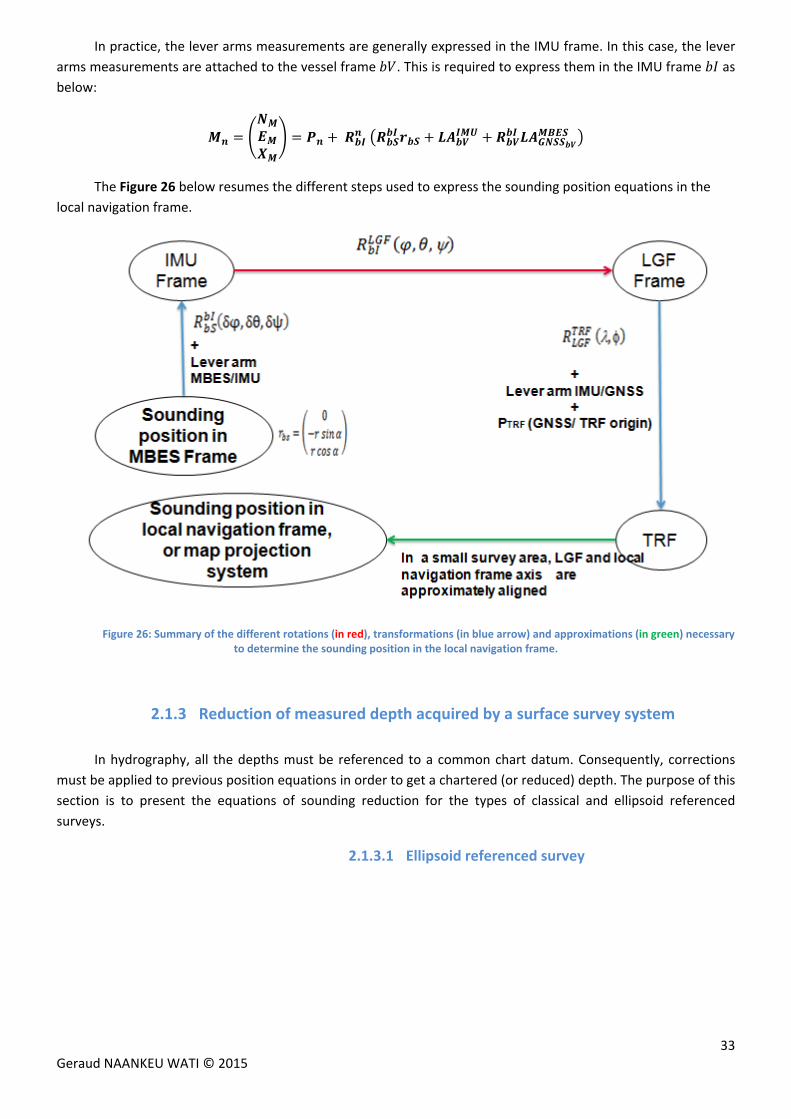
In practice, the lever arms measurements are generally expressed in the IMU frame. In this case, the lever
arms measurements are attached to the vessel frame . This is required to express them in the IMU frame as
below:
The Figure 26 below resumes the different steps used to express the sounding position equations in the
local navigation frame.
Figure 26: Summary of the different rotations (in red), transformations (in blue arrow) and approximations (in green) necessary to determine the sounding position in the local navigation frame.
2.1.3 Reduction of measured depth acquired by a surface survey system
In hydrography, all the depths must be referenced to a common chart datum. Consequently, corrections
must be applied to previous position equations in order to get a chartered (or reduced) depth. The purpose of this
section is to present the equations of sounding reduction for the types of classical and ellipsoid referenced
surveys.
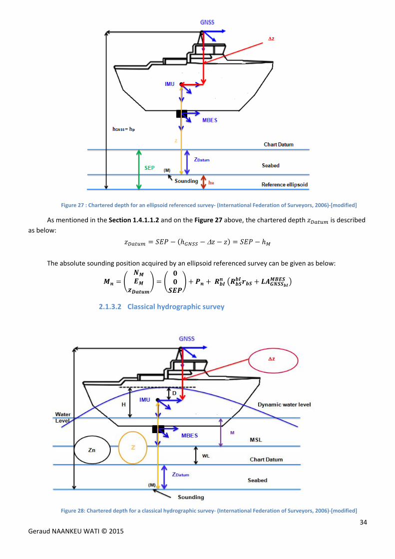
2.1.3.1 Ellipsoid referenced survey
34 Geraud NAANKEU WATI © 2015
Figure 27 : Chartered depth for an ellipsoid referenced survey‐ (International Federation of Surveyors, 2006)‐[modified]
As mentioned in the Section 1.4.1.1.2 and on the Figure 27 above, the chartered depth is described as below:
The absolute sounding position acquired by an ellipsoid referenced survey can be given as below:
2.1.3.2 Classical hydrographic survey
Figure 28: Chartered depth for a classical hydrographic survey‐ (International Federation of Surveyors, 2006)‐[modified]
35 Geraud NAANKEU WATI © 2015
As mentioned in the Section 1.4.1.1.1 and in the Figure 28 above, the chartered depth acquired by a
classical hydrographic survey is given by the formula below:
is the dynamic draft;
is the measured heave (Heave sensor);
is the measured tide;
is vertical offset between the MSL and the chart datum;
is the vertical offset between a sounding located at seabed and the IMU frame origin;
The vertical offset between a sounding located at the seabed and the IMU frame origin, is denoted . It is equal to the difference between the vertical offset between the seabed and the phase center position of GNSS
positioning system, denoted and the vertical offset between the phase center position of GNSS positioning
system and the IMU frame origin, denoted∆ .
∆
With:
∆ ; With,
The chartered depth becomes:
∆
The absolute sounding position acquired by a classical hydrographic survey can be given as below:
∆
As mentioned in the Section 1.1, the data acquired by the various sensors of a surface survey system are
not synchronous. Latency is introduced in some sensors of the system to take into account the time delay for
information transmission and computation. This creates a non‐negligible offset on the sounding position (Bjørn &
Einar, 2005). The purpose of this next section is to model the offset position of sounding due to the latency in
order to estimate the contribution of its latency measurement uncertainty on the sounding position during the
patch test. The measurement of latency by the classical patch test method is challenging. As an example, a
variation of latency GNSS/MBES of 0.53 s was observed between the start and the end of a bathymetry survey
around Cap Lopez‐Gabon in 2012.
Table 6: Calibration using the patch Test on the vessel Fugro IMPI‐Cap Lopez‐Gabon 2012
2.1.3.3 The dynamic equations of sounding position of surface survey system
The mathematical modeling of the sounding position offset due to the latency between the sensors has
been studied by (Seube, 2014) and (Bjørn & Einar, 2005) in a different way. The proposed approach in this section
is based on the approaches of (Seube, 2014) and (Bjørn & Einar, 2005) . It will allow improving the estimation of
Starting of project 15/12/2012 End of project 17/12/2012
Roll misalignment 2.35 ° 2.05°
Pitch misalignment ‐1° ‐1°
Yaw misalignment ‐1.0° ‐1.10°
Latency GNSS/MBES 0.38 s ‐0.15 s
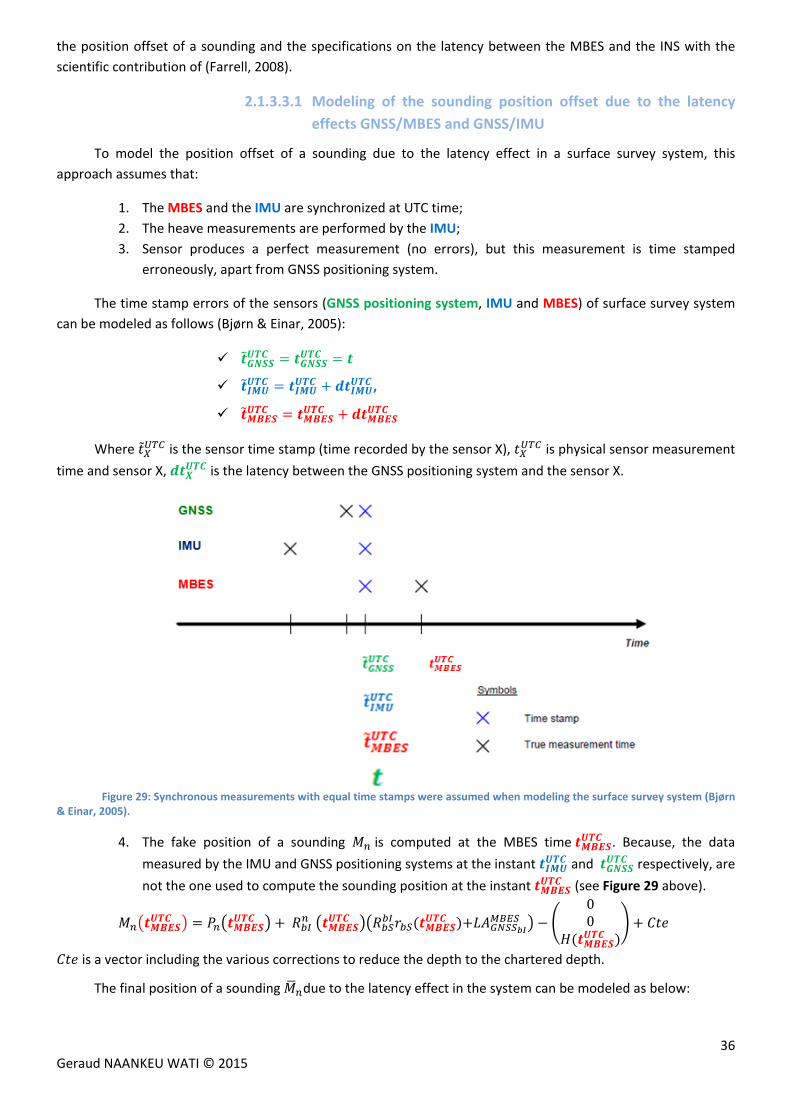
36 Geraud NAANKEU WATI © 2015
the position offset of a sounding and the specifications on the latency between the MBES and the INS with the
scientific contribution of (Farrell, 2008).
2.1.3.3.1 Modeling of the sounding position offset due to the latency
effects GNSS/MBES and GNSS/IMU
To model the position offset of a sounding due to the latency effect in a surface survey system, this
approach assumes that:
1. The MBES and the IMU are synchronized at UTC time;
2. The heave measurements are performed by the IMU;
3. Sensor produces a perfect measurement (no errors), but this measurement is time stamped
erroneously, apart from GNSS positioning system.
The time stamp errors of the sensors (GNSS positioning system, IMU and MBES) of surface survey system
can be modeled as follows (Bjørn & Einar, 2005):
,
Where is the sensor time stamp (time recorded by the sensor X), is physical sensor measurement
time and sensor X, is the latency between the GNSS positioning system and the sensor X.
Figure 29: Synchronous measurements with equal time stamps were assumed when modeling the surface survey system (Bjørn
& Einar, 2005).
4. The fake position of a sounding is computed at the MBES time . Because, the data
measured by the IMU and GNSS positioning systems at the instant and respectively, are
not the one used to compute the sounding position at the instant (see Figure 29 above).
00
is a vector including the various corrections to reduce the depth to the chartered depth.
The final position of a sounding due to the latency effect in the system can be modeled as below:
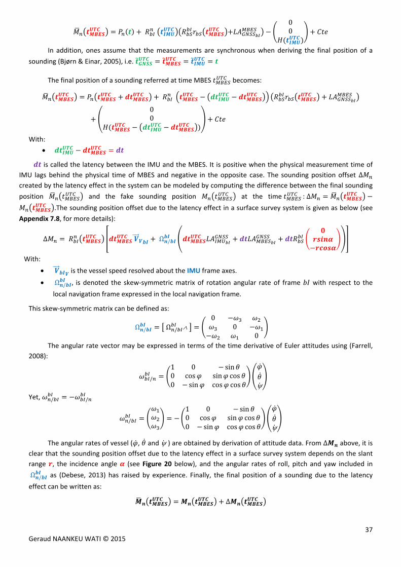
37 Geraud NAANKEU WATI © 2015
00
In addition, ones assume that the measurements are synchronous when deriving the final position of a
sounding (Bjørn & Einar, 2005), i.e.
The final position of a sounding referred at time MBES becomes:
00
With:
is called the latency between the IMU and the MBES. It is positive when the physical measurement time of
IMU lags behind the physical time of MBES and negative in the opposite case. The sounding position offset ∆
created by the latency effect in the system can be modeled by computing the difference between the final sounding
position and the fake sounding position at the time :∆
.The sounding position offset due to the latency effect in a surface survey system is given as below (see
Appendix 7.8, for more details):
∆ Ω /
With:
is the vessel speed resolved about the IMU frame axes.
Ω / , is denoted the skew‐symmetric matrix of rotation angular rate of frame with respect to the
local navigation frameexpressed in the local navigation frame.
This skew‐symmetric matrix can be defined as:
Ω / Ω / 0
00
The angular rate vector may be expressed in terms of the time derivative of Euler attitudes using (Farrell,
2008):
/
1 0 sin0 cos sin cos0 sin cos cos
Yet, / /
/
1 0 sin0 cos sin cos0 sin cos cos
The angular rates of vessel ( , and ) are obtained by derivation of attitude data. From ∆ above, it is
clear that the sounding position offset due to the latency effect in a surface survey system depends on the slant
range , the incidence angle (see Figure 20 below), and the angular rates of roll, pitch and yaw included in
Ω / as (Debese, 2013) has raised by experience. Finally, the final position of a sounding due to the latency
effect can be written as:
∆
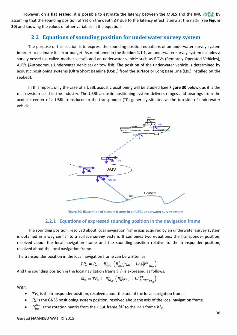
38 Geraud NAANKEU WATI © 2015
However, on a flat seabed, it is possible to estimate the latency between the MBES and the IMU by
assuming that the sounding position offset on the depth ∆ due to the latency effect is zero at the nadir (see Figure
20) and knowing the values of other variables in the equation.
2.2 Equationsofsoundingpositionforunderwatersurveysystem
The purpose of this section is to express the sounding position equations of an underwater survey system
in order to estimate its error budget. As mentioned in the Section 1.1.1, an underwater survey system includes a
survey vessel (so‐called mother vessel) and an underwater vehicle such as ROVs (Remotely Operated Vehicles),
AUVs (Autonomous Underwater Vehicles) or tow fish. The position of the underwater vehicle is determined by
acoustic positioning systems (Ultra Short Baseline (USBL) from the surface or Long Base Line (LBL) installed on the
seabed).
In this report, only the case of a USBL acoustic positioning will be studied (see Figure 30 below), as it is the
main system used in the industry. The USBL acoustic positioning system delivers ranges and bearings from the
acoustic center of a USBL transducer to the transponder (TP) generally situated at the top side of underwater
vehicle.
Figure 30: Illustration of sensors frames in an USBL underwater survey system
2.2.1 Equations of expressed sounding position in the navigation frame
The sounding position, resolved about local navigation frame axis acquired by an underwater survey system
is obtained in a way similar to a surface survey system. It combines two equations: the transponder position,
resolved about the local navigation frame and the sounding position relative to the transponder position,
resolved about the local navigation frame.
The transponder position in the local navigation frame can be written as:
And the sounding position in the local navigation frame is expressed as follows:
With:
is the transponder position, resolved about the axis of the local navigation frame.
is the GNSS positioning system position, resolved about the axis of the local navigation frame.
is the rotation matrix from the USBL frame to the IMU frame .
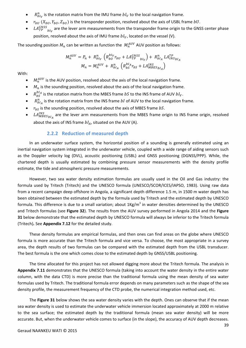
39 Geraud NAANKEU WATI © 2015
is the rotation matrix from the IMU frame to the local navigation frame.
, , is the transponder position, resolved about the axis of USBL frame .
are the lever arm measurements from the transponder frame origin to the GNSS center phase
position, resolved about the axis of IMU frame , located on the vessel (V).
The sounding position can be written as function the AUV position as follows:
With:
is the AUV position, resolved about the axis of the local navigation frame.
is the sounding position, resolved about the axis of the local navigation frame.
is the rotation matrix from the MBES frame to the INS frame of AUV .
is the rotation matrix from the INS frame of AUV to the local navigation frame.
is the sounding position, resolved about the axis of MBES frame .
are the lever arm measurements from the MBES frame origin to INS frame origin, resolved
about the axis of INS frame , situated on the AUV (A).
2.2.2 Reduction of measured depth
In an underwater surface system, the horizontal position of a sounding is generally estimated using an
inertial navigation system integrated in the underwater vehicle, coupled with a wide range of aiding sensors such
as the Doppler velocity log (DVL), acoustic positioning (USBL) and GNSS positioning (DGNSS/PPP). While, the
chartered depth is usually estimated by combining pressure sensor measurements with the density profile
estimate, the tide and atmospheric pressure measurements.
However, two sea water density estimation formulas are usually used in the Oil and Gas industry: the
formula used by Tritech (Tritech) and the UNESCO formula (UNESCO/SCOR/ICES/IAPSO, 1983). Using raw data
from a recent campaign deep offshore in Angola, a significant depth difference 1.5 m, in 1500 m water depth has
been obtained between the estimated depth by the formula used by Tritech and the estimated depth by UNESCO
formula. This difference is due to a small variation; about 1Kg/m3 in water densities determined by the UNESCO
and Tritech formulas (see Figure 32). The results from the AUV survey performed in Angola 2014 and the Figure
31 below demonstrate that the estimated depth by UNESCO formula will always be inferior to the Tritech formula
(Tritech). See Appendix 7.12 for the detailed study.
These density formulas are empirical formulas, and then ones can find areas on the globe where UNESCO
formula is more accurate than the Tritech formula and vice versa. To choose, the most appropriate in a survey
area, the depth results of two formulas can be compared with the estimated depth from the USBL transducer.
The best formula is the one which comes close to the estimated depth by GNSS/USBL positioning.
The time allocated for this project has not allowed digging more about the Tritech formula. The analysis in
Appendix 7.11 demonstrates that the UNESCO formula (taking into account the water density in the entire water
column, with the data CTD) is more precise than the traditional formula using the mean density of sea water
formulas used by Tritech. The traditional formula error depends on many parameters such as the shape of the sea
density profile, the measurement frequency of the CTD probe, the numerical integration method used, etc.
The Figure 31 below shows the sea water density varies with the depth. Ones can observe that if the mean
sea water density is used to estimate the underwater vehicle immersion located approximately at 2000 m relative
to the sea surface; the estimated depth by the traditional formula (mean sea water density) will be more
accurate. But, when the underwater vehicle comes to surface (in the slope), the accuracy of AUV depth decreases.
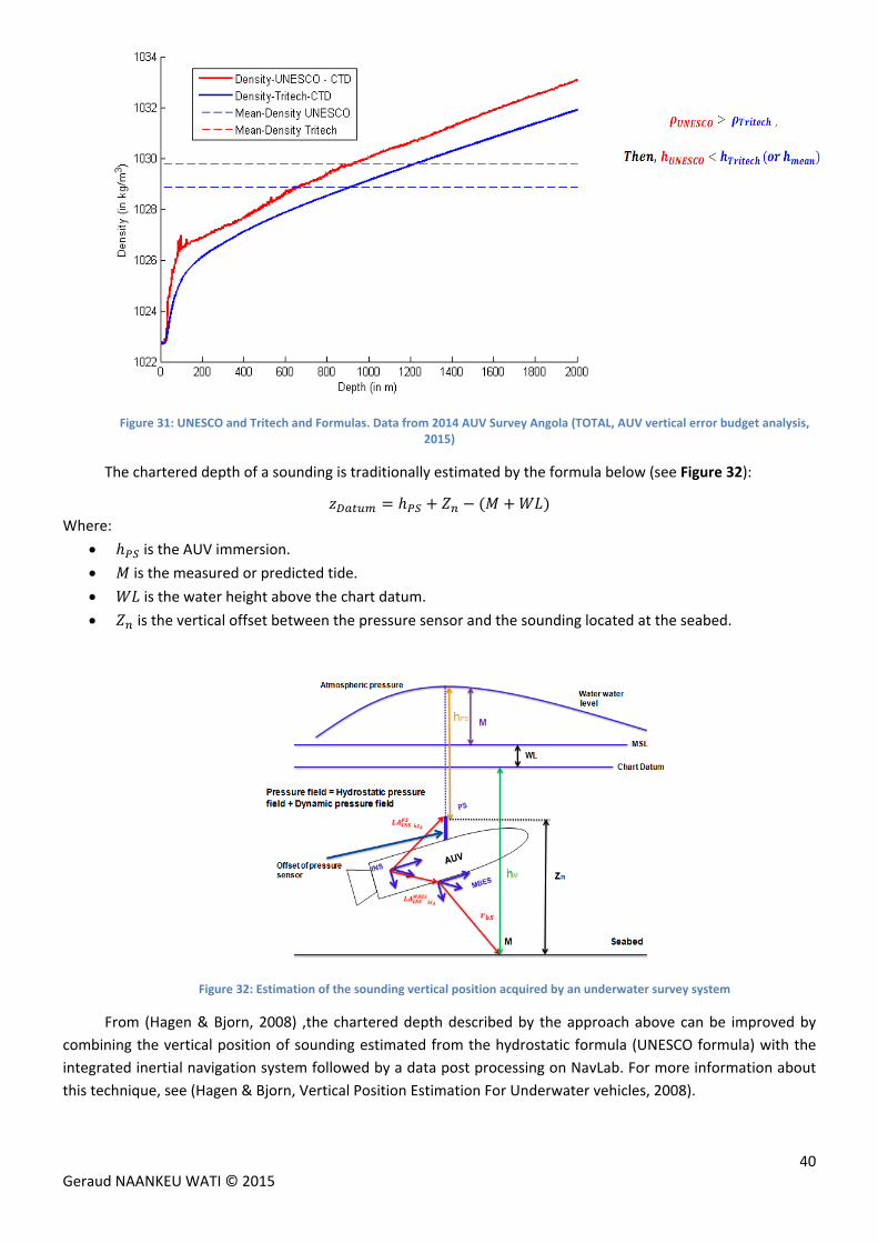
40 Geraud NAANKEU WATI © 2015
Figure 31: UNESCO and Tritech and Formulas. Data from 2014 AUV Survey Angola (TOTAL, AUV vertical error budget analysis, 2015)
The chartered depth of a sounding is traditionally estimated by the formula below (see Figure 32):
Where:
is the AUV immersion.
is the measured or predicted tide.
is the water height above the chart datum.
is the vertical offset between the pressure sensor and the sounding located at the seabed.
Figure 32: Estimation of the sounding vertical position acquired by an underwater survey system
From (Hagen & Bjorn, 2008) ,the chartered depth described by the approach above can be improved by
combining the vertical position of sounding estimated from the hydrostatic formula (UNESCO formula) with the
integrated inertial navigation system followed by a data post processing on NavLab. For more information about
this technique, see (Hagen & Bjorn, Vertical Position Estimation For Underwater vehicles, 2008).
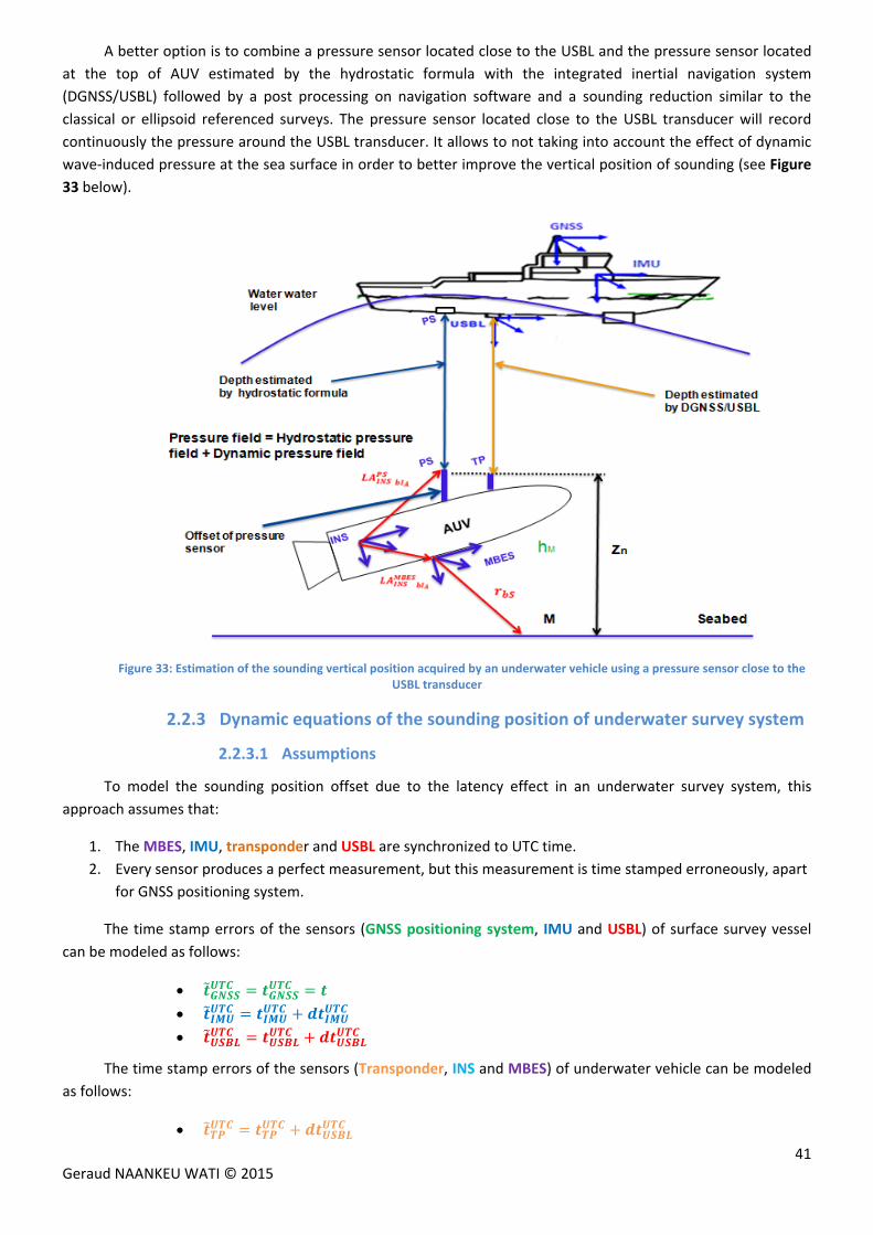
41 Geraud NAANKEU WATI © 2015
A better option is to combine a pressure sensor located close to the USBL and the pressure sensor located
at the top of AUV estimated by the hydrostatic formula with the integrated inertial navigation system
(DGNSS/USBL) followed by a post processing on navigation software and a sounding reduction similar to the
classical or ellipsoid referenced surveys. The pressure sensor located close to the USBL transducer will record
continuously the pressure around the USBL transducer. It allows to not taking into account the effect of dynamic
wave‐induced pressure at the sea surface in order to better improve the vertical position of sounding (see Figure
33 below).
Figure 33: Estimation of the sounding vertical position acquired by an underwater vehicle using a pressure sensor close to the USBL transducer
2.2.3 Dynamic equations of the sounding position of underwater survey system
2.2.3.1 Assumptions
To model the sounding position offset due to the latency effect in an underwater survey system, this
approach assumes that:
1. The MBES, IMU, transponder and USBL are synchronized to UTC time.
2. Every sensor produces a perfect measurement, but this measurement is time stamped erroneously, apart
for GNSS positioning system.
The time stamp errors of the sensors (GNSS positioning system, IMU and USBL) of surface survey vessel
can be modeled as follows:
The time stamp errors of the sensors (Transponder, INS and MBES) of underwater vehicle can be modeled
as follows:
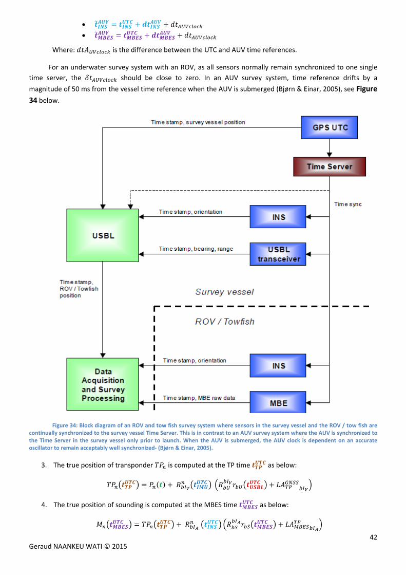
42 Geraud NAANKEU WATI © 2015
Where: is the difference between the UTC and AUV time references.
For an underwater survey system with an ROV, as all sensors normally remain synchronized to one single
time server, the should be close to zero. In an AUV survey system, time reference drifts by a
magnitude of 50 ms from the vessel time reference when the AUV is submerged (Bjørn & Einar, 2005), see Figure
34 below.
Figure 34: Block diagram of an ROV and tow fish survey system where sensors in the survey vessel and the ROV / tow fish are continually synchronized to the survey vessel Time Server. This is in contrast to an AUV survey system where the AUV is synchronized to the Time Server in the survey vessel only prior to launch. When the AUV is submerged, the AUV clock is dependent on an accurate oscillator to remain acceptably well synchronized‐ (Bjørn & Einar, 2005).
3. The true position of transponder is computed at the TP time as below:
4. The true position of sounding is computed at the MBES time as below:
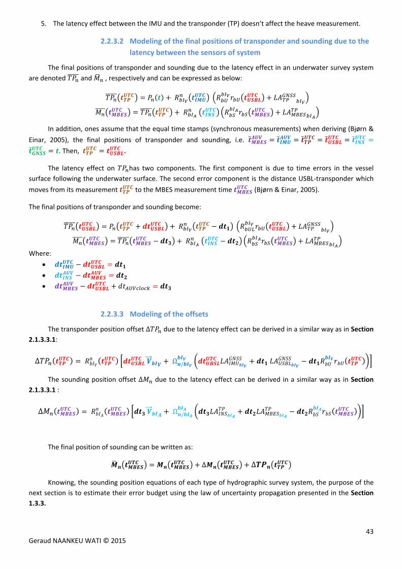
43 Geraud NAANKEU WATI © 2015
5. The latency effect between the IMU and the transponder (TP) doesn’t affect the heave measurement.
2.2.3.2 Modeling of the final positions of transponder and sounding due to the
latency between the sensors of system
The final positions of transponder and sounding due to the latency effect in an underwater survey system
are denoted and , respectively and can be expressed as below:
In addition, ones assume that the equal time stamps (synchronous measurements) when deriving (Bjørn &
Einar, 2005), the final positions of transponder and sounding, i.e.
. Then, .
The latency effect on has two components. The first component is due to time errors in the vessel
surface following the underwater surface. The second error component is the distance USBL‐transponder which
moves from its measurement to the MBES measurement time (Bjørn & Einar, 2005).
The final positions of transponder and sounding become:
Where:
2.2.3.3 Modeling of the offsets
The transponder position offset ∆ due to the latency effect can be derived in a similar way as in Section
2.1.3.3.1:
∆ Ω /
The sounding position offset ∆ due to the latency effect can be derived in a similar way as in Section
2.1.3.3.1 :
∆ Ω /
The final position of sounding can be written as:
∆ ∆
Knowing, the sounding position equations of each type of hydrographic survey system, the purpose of the
next section is to estimate their error budget using the law of uncertainty propagation presented in the Section
1.3.3.
44 Geraud NAANKEU WATI © 2015
3. ERRORBUDGETESTIMATIONFORHYDROGRAPHICSURVEYSYSTEMS
The objective of this section is to estimate the measurement uncertainty of the sounding position acquired
by underwater and surface survey systems. It will also enable analyzing the effect of each sensor uncertainties on
the sounding position.
3.1 Errorbudgetestimationforsurfacesurveysystem
The sounding position acquired by a surface survey system depends on several parameters measured by
various sensors (GNSS positioning system, MBES, IMU, etc). Each measurement has an uncertainty. The
uncertainties are then combined to estimate the measurement uncertainty of the sounding position, using the
law of uncertainty propagation described in the Section 1.3.3. The sensors uncertainties are summarized in
Appendix 7.9.
3.1.1.1 Algorithm of error budget estimation for surface survey system
The algorithm assumptions of error budget estimation for surface survey system are:
1. All the parameters uncertainties measured by the sensors of system are well known. The uncertainties of
angle measurements must be converted in radians and the uncertainties of distance measurements must
be converted in meters.
2. All parameters uncertainties are normally distributed and uncorrelated. This assumption is not true as all
the measurements acquired by a same sensor must be correlated. For instance, there is a correlation
between the measurements of roll, pitch and yaw estimated by the IMU. But, there is no a correlation
between the roll measured by a MRU and the yaw measured by the Gyrocompass. This assumption has
been done as the correlation values between the parameters of a sensor aren’t provided by the
manufacturers. With more intensive mathematic considerations, it is will possible for them to estimate
the correlation between the various measurements of a sensor.
3. The sounding horizontal position uncertainty at 1 is 2| , |. The
covariance term is in absolute value as it is non negligible. When N and E position coordinates vary in the
opposite direction, the covariance term is negative and affects significantly the uncertainty position. This
assumption allows having more realistic results.
4. The measurement uncertainty model of the MBES used is this proposed by (Hammerstad, 2001).
The algorithm of error budget estimation has been developed on EXCEL (VBA). Most functions have been
written on Matlab and then imported into EXCEL (VBA). It is also possible to import these functions (position
equations and error budget) in FORTRAN, C, and PYTHON languages to easily implement the algorithm in
hydrographic data acquisition, navigation and processing softwares. This tool can be used on many operating
systems including Windows, Windows Phone, Android and MAC OSX.
It is important to notice that this algorithm takes into account the covariance between the fake position of
sounding (without latency) and the position offset of the sounding due to the latency effect (or time stamp error)
in the system.
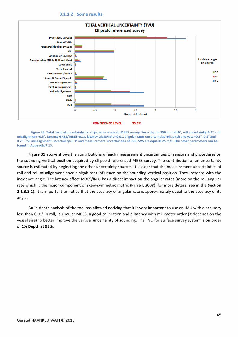
45 Geraud NAANKEU WATI © 2015
3.1.1.2 Some results
Figure 35: Total vertical uncertainty for ellipsoid referenced MBES survey. For a depth=250 m, roll=6°, roll uncertainty=0.1°, roll misalignment=0.5°, Latency GNSS/MBES=0.1s, latency GNSS/IMU=0.01, angular rates uncertainties roll, pitch and yaw =0.1°, 0.1° and 0.2 °, roll misalignment uncertainty=0.1° and measurement uncertainties of SVP, SVS are equal 0.25 m/s. The other parameters can be found in Appendix 7.13.
Figure 35 above shows the contributions of each measurement uncertainties of sensors and procedures on
the sounding vertical position acquired by ellipsoid referenced MBES survey. The contribution of an uncertainty
source is estimated by neglecting the other uncertainty sources. It is clear that the measurement uncertainties of
roll and roll misalignment have a significant influence on the sounding vertical position. They increase with the
incidence angle. The latency effect MBES/IMU has a direct impact on the angular rates (more on the roll angular
rate which is the major component of skew‐symmetric matrix (Farrell, 2008), for more details, see in the Section
2.1.3.3.1). It is important to notice that the accuracy of angular rate is approximately equal to the accuracy of its
angle.
An in‐depth analysis of the tool has allowed noticing that it is very important to use an IMU with a accuracy
less than 0.01° in roll, a circular MBES, a good calibration and a latency with millimeter order (it depends on the
vessel size) to better improve the vertical uncertainty of sounding. The TVU for surface survey system is on order
of 1% Depth at 95%.
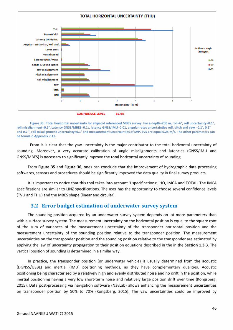
46 Geraud NAANKEU WATI © 2015
Figure 36 : Total horizontal uncertainty for ellipsoid referenced MBES survey. For a depth=250 m, roll=6°, roll uncertainty=0.1°, roll misalignment=0.5°, Latency GNSS/MBES=0.1s, latency GNSS/IMU=0.01, angular rates uncertainties roll, pitch and yaw =0.1°, 0.1° and 0.2 °, roll misalignment uncertainty=0.1° and measurement uncertainties of SVP, SVS are equal 0.25 m/s. The other parameters can be found in Appendix 7.13.
From it is clear that the yaw uncertainty is the major contributor to the total horizontal uncertainty of
sounding. Moreover, a very accurate calibration of angle misalignments and latencies (GNSS/IMU and
GNSS/MBES) is necessary to significantly improve the total horizontal uncertainty of sounding.
From Figure 35 and Figure 36, ones can conclude that the improvement of hydrographic data processing
softwares, sensors and procedures should be significantly improved the data quality in final survey products.
It is important to notice that this tool takes into account 3 specifications: IHO, IMCA and TOTAL. The IMCA
specifications are similar to LINZ specifications. The user has the opportunity to choose several confidence levels
(TVU and THU) and the MBES shape (linear and circular).
3.2 Errorbudgetestimationofunderwatersurveysystem
The sounding position acquired by an underwater survey system depends on lot more parameters than
with a surface survey system. The measurement uncertainty on the horizontal position is equal to the square root
of the sum of variances of the measurement uncertainty of the transponder horizontal position and the
measurement uncertainty of the sounding position relative to the transponder position. The measurement
uncertainties on the transponder position and the sounding position relative to the transponder are estimated by
applying the law of uncertainty propagation to their position equations described in the in the Section 1.3.3. The
vertical position of sounding is determined in a similar way.
In practice, the transponder position (or underwater vehicle) is usually determined from the acoustic
(DGNSS/USBL) and inertial (IMU) positioning methods, as they have complementary qualities. Acoustic
positioning being characterized by a relatively high and evenly distributed noise and no drift in the position, while
inertial positioning having a very low short‐term noise and relatively large position drift over time (Kongsberg,
2015). Data post‐processing via navigation software (NavLab) allows enhancing the measurement uncertainties
on transponder position by 50% to 70% (Kongsberg, 2015). The yaw uncertainties could be improved by
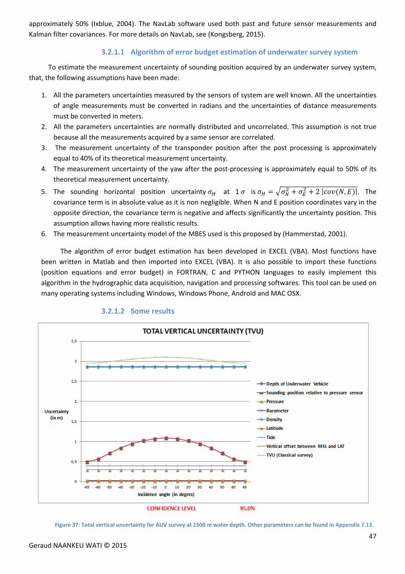
47 Geraud NAANKEU WATI © 2015
approximately 50% (Ixblue, 2004). The NavLab software used both past and future sensor measurements and
Kalman filter covariances. For more details on NavLab, see (Kongsberg, 2015).
3.2.1.1 Algorithm of error budget estimation of underwater survey system
To estimate the measurement uncertainty of sounding position acquired by an underwater survey system,
that, the following assumptions have been made:
1. All the parameters uncertainties measured by the sensors of system are well known. All the uncertainties
of angle measurements must be converted in radians and the uncertainties of distance measurements
must be converted in meters.
2. All the parameters uncertainties are normally distributed and uncorrelated. This assumption is not true
because all the measurements acquired by a same sensor are correlated.
3. The measurement uncertainty of the transponder position after the post processing is approximately
equal to 40% of its theoretical measurement uncertainty.
4. The measurement uncertainty of the yaw after the post‐processing is approximately equal to 50% of its
theoretical measurement uncertainty.
5. The sounding horizontal position uncertainty at 1 is 2| , |. The
covariance term is in absolute value as it is non negligible. When N and E position coordinates vary in the
opposite direction, the covariance term is negative and affects significantly the uncertainty position. This
assumption allows having more realistic results.
6. The measurement uncertainty model of the MBES used is this proposed by (Hammerstad, 2001).
The algorithm of error budget estimation has been developed in EXCEL (VBA). Most functions have
been written in Matlab and then imported into EXCEL (VBA). It is also possible to import these functions
(position equations and error budget) in FORTRAN, C and PYTHON languages to easily implement this
algorithm in the hydrographic data acquisition, navigation and processing softwares. This tool can be used on
many operating systems including Windows, Windows Phone, Android and MAC OSX.
3.2.1.2 Some results
Figure 37: Total vertical uncertainty for AUV survey at 1500 m water depth. Other parameters can be found in Appendix 7.13.
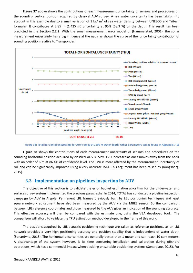
48 Geraud NAANKEU WATI © 2015
Figure 37 above shows the contributions of each measurement uncertainty of sensors and procedures on
the sounding vertical position acquired by classical AUV survey. A sea water uncertainty has been taking into
account in this example due to a small variation of 1 kg/ m3 of sea water density between UNESCO and Tritech
formulas. It contributes at 2.85 m (1.425 m) uncertainty at 95% (68.3 %) on the depth. This result has been
predicted in the Section 2.2.2. With the sonar measurement error model of (Hammerstad, 2001), the sonar
measurement uncertainty has a big influence at the nadir as shown the curve of the uncertainty contribution of
sounding position relative to Transponder.
Figure 38: Total horizontal uncertainty for AUV survey at 1500 m water depth. Other parameters can be found in Appendix 7.13
Figure 38 shows the contributions of each measurement uncertainty of sensors and procedures on the
sounding horizontal position acquired by classical AUV survey. TVU increases as ones moves away from the nadir
with an order of 6 m at 86.4% of confidence level. The TVU is more affected by the measurement uncertainty of
roll and can be significantly improved using a very accurate IMU. This argument has been raised by (Kongsberg,
2015).
3.3 ImplementationonpipelinesinspectionbyAUV
The objective of this section is to validate the error budget estimation algorithm for the underwater and
surface survey system implemented the previous paragraphs. In 2014, TOTAL has conducted a pipeline inspection
campaign by AUV in Angola. Permanent LBL frames previously built by LBL positioning techniques and least
square network adjustment have also been measured by the AUV via the MBES sensor. So the comparison
between LBL reference coordinates and those measured by the AUV gives an indication of the sounding accuracy.
This effective accuracy will then be compared with the estimate one, using the VBA developed tool. The
comparison will afford to validate the TPU estimation method developed in the frame of this work.
The positions acquired by LBL acoustic positioning technique are taken as reference positions, as an LBL
network provides a very high positioning accuracy and position stability that is independent of water depth
(Sonardyne, 2015). The horizontal uncertainties are generally better than 1‐meter and can reach 10 centimeters.
A disadvantage of the system however, is its time consuming installation and calibration during offshore
operations, which has a commercial impact when deciding on suitable positioning systems (Sonardyne, 2015). For
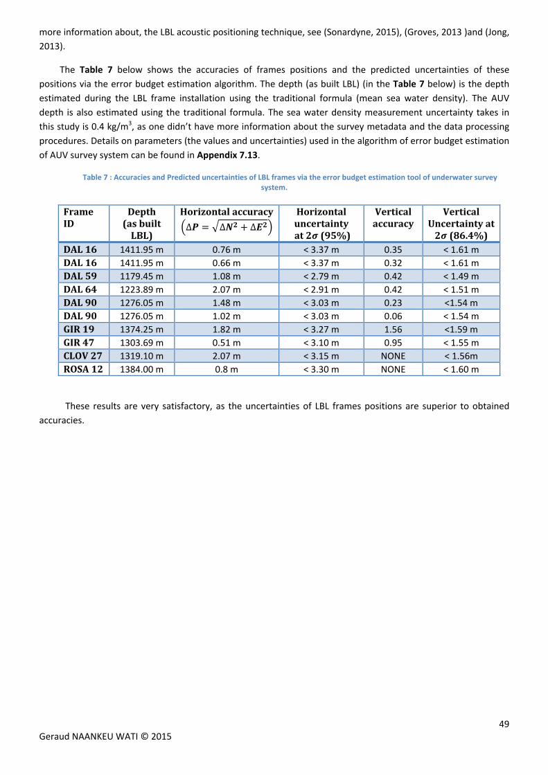
49 Geraud NAANKEU WATI © 2015
more information about, the LBL acoustic positioning technique, see (Sonardyne, 2015), (Groves, 2013 )and (Jong,
2013).
The Table 7 below shows the accuracies of frames positions and the predicted uncertainties of these
positions via the error budget estimation algorithm. The depth (as built LBL) (in the Table 7 below) is the depth
estimated during the LBL frame installation using the traditional formula (mean sea water density). The AUV
depth is also estimated using the traditional formula. The sea water density measurement uncertainty takes in
this study is 0.4 kg/m3, as one didn’t have more information about the survey metadata and the data processing
procedures. Details on parameters (the values and uncertainties) used in the algorithm of error budget estimation
of AUV survey system can be found in Appendix 7.13.
Table 7 : Accuracies and Predicted uncertainties of LBL frames via the error budget estimation tool of underwater survey system.
These results are very satisfactory, as the uncertainties of LBL frames positions are superior to obtained
accuracies.
FrameID
Depth(asbuiltLBL)
∆ ∆ ∆
Horizontal accuracy Horizontaluncertaintyat2 (95%)
Verticalaccuracy
VerticalUncertaintyat2 (86.4%)
DAL16 1411.95 m 0.76 m < 3.37 m 0.35 < 1.61 m
DAL16 1411.95 m 0.66 m < 3.37 m 0.32 < 1.61 m
DAL59 1179.45 m 1.08 m < 2.79 m 0.42 < 1.49 m
DAL64 1223.89 m 2.07 m < 2.91 m 0.42 < 1.51 m
DAL90 1276.05 m 1.48 m < 3.03 m 0.23 <1.54 m
DAL90 1276.05 m 1.02 m < 3.03 m 0.06 < 1.54 m
GIR19 1374.25 m 1.82 m < 3.27 m 1.56 <1.59 m
GIR47 1303.69 m 0.51 m < 3.10 m 0.95 < 1.55 m
CLOV27 1319.10 m 2.07 m < 3.15 m NONE < 1.56m
ROSA12 1384.00 m 0.8 m < 3.30 m NONE < 1.60 m
50 Geraud NAANKEU WATI © 2015
CONCLUSIONANDOUTLOOK
The objective of this final year project was to study and compare different methods of error budget
estimation used by TOTAL contractors and other existing tools on the market, in order to better qualify the
hydrographic data. The outcome of this work can be summarized as follows:
Improvement of the sounding position acquired by the underwater and surface survey systems.
Improvement of the error budget estimation algorithm for underwater and surface survey systems. The
main added value is:
The consideration of all the couplings between the errors by the differentiation and the errors
propagation of a MBES functional model.
The consideration of time‐stamping error.
The consideration of couplings IMU surface /MBES, MBES/IMU (underwater) and time‐stamping.
Demonstration that a yaw misalignment between the IMU (or MRU and Gyrocompass) and the MBES
influences the vertical position of sounding,
Identification of the automatic calibration methods importance relative to the classical patch test method,
Clarification of the issue related to the methods of conversion from pressure to depth.
The deliverables of this study are the implementation of error budget estimation algorithms on EXCEL
(VBA) applied to underwater and surface survey systems and a report (this document) detailing the workflow of
the study. These supports will be used by TOTAL to evaluate the technical aspects of contractor proposals, in
order to better qualify acquired data and monitor the exploration‐production activities. The error budget
estimation and position equations algorithms for underwater and surface survey systems can be easily imported
in FORTRAN, C and PYTHON in order to quickly update hydrographic data acquisition, navigation and processing
softwares. They can be used on many operating systems including Windows, Windows Phone, Android and MAC
OSX. An implementation of error budget estimation tool has been done from the data of the inspection campaign
of pipelines by AUV in Angola in 2014. The results obtained are satisfactory.
Graceful thanks for the members of the hydrographic survey community involved in this project for their
insightful and constructive help. This objective could be achieved through the combined efforts of several people
of the hydrographic survey community. This report benefited from comments from: Jean‐baptiste GELDOF
(TOTAL), Vincent LATRON (TOTAL), Marie‐Laure GEAI (TOTAL), Nicolas SEUBE (CIDCO), Frederic AUGER (TOTAL),
Pierre BOSSER (ENSTA Bretagne), Patricia GASPAR (CARIS), Marc KEBBEL (FUGRO), Nathalie DEBESE (ENSTA
Bretagne), Arnaud VIDAL (TOTAL), Chris MALZONE (QPS), Emilie BLANCART (TOTAL), Rabine KEYETIEU (CIDCO),
Jeppe NIELSEN (EIVA) and Colin CAMERON (DOF Subsea). The equations developed in this report have been
validated by Nicolas SEUBE (Doctorate in Mathematics, President of FIG/IHO/ICA International Board on
Standards of Competence for Hydrographic Surveyors and Nautical Cartographers, Scientific Director at CIDCO).
This work is very likely to be published in scientific paper.
At the same time as this internship occurred, CARIS introduced a new Sound Velocity Correction algorithm
in HIPS and SIPS that significantly improves the results in deep water (the sounding position equations, the error
budget and the calibration methods). Also, CIDCO is developing an automatic calibration tool (MBES). Their
preliminary results are very satisfactory and should improve the uncertainties of the sounding position.
Moreover, FUGRO is developing a new GNSS positioning technique (PPP‐IAR) which significantly improves the
offshore positioning.
A major axis of improvement for MBES manufacturers would be to improve their sensors by cancelling the
roll compensation (as this simplification isn’t valid when there is a misalignment between the IMU and the MBES).
Future research may focus on the improvement of sensors accuracies (IMU, MBES, USBL, etc), hydrographic data
processing softwares, procedures (sounding reduction, uncertainty estimation of predicted tide) in order to
answer to needs of hydrographic survey community (oil and gas industry, hydrographic services, etc.).
51 Geraud NAANKEU WATI © 2015
4. BIBLIOGRAPHY
Barry, T., & Chris, K. (1994). Guidelines for Evaluating and Expressing the Uncertainty of NIST
Measurement Results. Retrieved May 17, 2015, from http://physics.nist.gov/Pubs/guidelines/sec5.html#5.2
Bjørn, J., & Einar, B. (2005). Time Referencing in Offshore Survey Systems. FFI.
Bjørn, J., & Einar, B. (2005). Time Referencing in Offshore Survey Systems. FFI.
Bjorn, J., & Kenneth, G. (1998). POSITIIONING ACCURACY FOR THE HUGIN DETAILED SEABED MAPPING
UUV. Norwegian Defence Research Establishment (FFI). Kjeller,Norway: OCEANS'98 Conference Proceedings 1.
Bosser, P. (2013). GNSS: Systèmes Globaux de Positionnement par Satellite. Support de Cours de Géodésie
à l'Ecole Nationale des Sciences Géographiques ( ENSG).
Calder, B. (2003). Automated Statistical Processing of Multibeam Echosounder Data. Hydro Review.
Canadian Hydrographic Servicce. (2012, Février). Fisheries and Oceans Canada. Retrieved Mai 6, 2015,
from http://www.charts.gc.ca/data‐gestion/hydrographic/bathymetric‐traitement‐fra.pdf
CARIS. (2004). Total Propagated Uncertainty Computation. Retrieved July 20, 2015, from CARIS:
http://www.caris.com/tpu/
Cenac, J.‐O. (1997). Utilisation des modèles de marée issus d'altimétrie radar en sismique 3D marine.
Mémoire d'ingénieur de l'ESGT pour le Groupe TOTAL.
Debese, N. (2013). Bathymétrie. Sondeurs,traitement de données,modèles numériques de terrain. Paris:
Ellipses Editions Marketing S.A.
Exell, R. H. (2001). Error Analysis. Retrieved May 15, 2015, from
http://www.jgsee.kmutt.ac.th/exell/PracMath/ErrorAn.htm
Farrell, J. (2008). Aided Navigation: GPS with High Rate Sensors. New York: McGraw‐Hill.
Forence, I. (2014). Underwater Acoustic Positioning. Kongsberg. Scotland: Kongsberg.
Fugro. (2013). HUGIN 3000 AUV Error Budget.
Gonçalves, & Jalobeanu, A. (2011). LiDAR bore‐sight calibration:a study comparative.
Groves, P. D. (2013). PRINCIPLES OF GNSS, INERTIAL, AND MULTISENSOR INTEGRATED NAVIGATION
SYSTEMS (Second Edition ed.). Houston: Artech House.
Groves, P. D. (2013 ). Principles of GNSS, Inertial, and Multisensor Integrated Navigation Systems (Second
Edition ed.). Houston: Artech House.
Hagen, O. K. (2008). Fom Pressure to Depth‐Estimation of underwater vertical position. Norwegian
Defence Research Establishment‐FFI.
hagen, O. K. (2008). From pressure to depth‐Estimation of underwater vertical position.
Hagen, O. K. (2006). TerrLab ‐ a generic simulation and post‐processing tool for terrain referenced
navigation. Norwegian Defence Research Establishment, Norway.
52 Geraud NAANKEU WATI © 2015
Hagen, O. K., & Bjorn. (2008). Vertical Position Estimation For Underwater vehicles.
Hammerstad, E. (2001). Multibeam Echo Sounder Accuracy. EM Technical Note, Kongsberg Simrad AS.
Hansen, R. E. (2012). Introduction to sonar. Oslo.
Hare, R. (2004, July). Retrieved June 1, 2015, from
http://www.google.fr/url?url=ftp://moray.dms.usm.edu/archived/cube/8a_Hare%2520on%2520CUBE%2520%26
%2520NavSurface.ppt&rct=j&frm=1&q=&esrc=s&sa=U&ei=PDhsVZ35JZKf7gbb4YDoCQ&ved=0CBQQFjAA&usg=AF
QjCNEntKcc6bz‐4HFXOyExYWuc5m0TQw
Hare, R. ( 2001). Error Budget Analysis for US NAVAL Oceanographic Office (NAVOCEANO) Hydrographic
Survey Systems. Mississippi: University Mississippi.
Huang M, Z. G. (2002). The influence of carrier's attitude and the position reduction in multibeam
echosounder and airbone laser depth sounding. International Hydrographic Review for publication in the spring
2002 edition.
IGN. (2008). Systèmes de coordonnées.
IMCA. (2011). Guidelines for the GNSS positioning in the oil & gas industry.
IMCA. (2011). Guidelines for the GNSS positioning in the oil & gas industry.
In‐Situ. (2000). Water Level Accuracy and Correcting for Errors. Retrieved May 27, 2015
International Federation of Surveyors. (2006). FIG Guide on the development of Vertical Reference Surface
for Hydrography. Denmark.
Internationale Organisation Hydrographique. (2011). Publication spéciale n°44 : Normes OHI pour les levés
hydrographiques (première parution en 2008, révisée en 2011) (Vol. 5ème edition). Monaco: Editions Bureau
Hydrographique International.
Internationale, O. H. (2011). Publication spéciale n°44 : Normes OHI pour les levés hydrographiques
(première parution en 2008, révisée en 2011) (Vol. 5ème edition). Monaco: Editions Bureau Hydrographique
International.
IOGP. (2012). Geomatics Guidance ‐ Coordinate Conversions and Transformations including Formulas (Vol.
I).
Ixblue. (2004). Ixblue. Retrieved July 20, 2015, from http://www.ixblue.com/products/usbl‐positioning‐
systems
Jason, B., & Rob, H. (2011, June 18). Hydro International. Retrieved June 1, 2015, from http://www.hydro‐
international.com/issues/articles/id1290‐Solving_the_Uncertainty_Management_Puzzle.html
JCGM. (2008). Evaluation of measurement data ‐ Guide to the expression of uncertainty in measurement
(Vol. I).
Jekeli, C. (2000). Inertial Navigation Systems with Geodetic Applications.
Jong, K. D. (2013). Offshore Positioning. Cours à l'ENSTA Bretagne, spécialité Hydrographie, Brest.
Knippers. (2009, 2014). Geometric Aspects of Mapping. Retrieved May 14, 2015, from
http://kartoweb.itc.nl/geometrics/coordinate%20transformations/coordtrans.html
53 Geraud NAANKEU WATI © 2015
Kongsberg. (2015). Retrieved July 7, 2015, from
http://www.km.kongsberg.com/ks/web/NOKBG0240.nsf/AllWeb/CD81027CDE8C21ADC125721800428002?Open
Document
Kongsberg. (2015). Retrieved July 18, 2015, from
http://www.km.kongsberg.com/ks/web/nokbg0240.nsf/AllWeb/BC10CC31F901DECAC125721800372543?OpenD
ocument
Kongsberg. (2015). Retrieved June 31, 2015, from
http://www.km.kongsberg.com/ks/web/NOKBG0240.nsf/AllWeb/19F6F6FD9513D33AC1257218004646BA?Open
Document
Kongsberg. (n.d.). High Presicion Acoustic Positioning ‐ HIPAP. Retrieved July 20, 2015, from
http://www.km.kongsberg.com/ks/web/nokbg0397.nsf/AllWeb/D3F9B693E19302BBC12571B6003DD0AE/$file/H
iPAP_Family_brochure_v3_lowres.pdf?OpenElement
Ladroit, Y. (2012). Amélioration des méthodes de détection et de qualification des sondes pour les sondeurs
multifaisceaux bathymétriques. Université européenne de Bretagne.
Legris, M. (2014). Bathymétrie. Cours à l'ENSTA Bretagne, spécialité Hydrographie, Brest.
Leitch, R. (2014). Survey Sensors. Scotland: Nautronix.
Lurton, X. (2001). Précision de mesure des sonars bathymétrique en fonction du rapport signal/bruit.
Magne, M., Kenneth, G., & Bjorn, J. (2004). Integrating DGPS‐USBL position measurements with inertial
navigation in the HUGIN 3000 AUV. Kongsberg Simrad‐Norwegian Defence Research Establishment. Norway:
Norwegian Defence Research Establishment.
Massard, E. (2007). Incertitudes de mesures bathymétriques: évaluation, valisation et application sur les
levés bathymétriques de la Seudre et sur les bancs ostréicoles du Bassin de Marennes‐Oléron. Rapport de Stage‐
Université de La Rochelle.
Maybeck, P. (1973). Wander azimuth implementation algorithm for a strapdown inertial system.
Moller, E. (2012). Acoustic (Subsea) Positioning Systems. Presentation at Hydrofest 2012, Sonardyne,
Scotland.
Nicolle, A. (2014). Marée. Cours à l'ENSTA Bretagne, spécialité Hydrographie, Brest.
NOAA. (2013, Octobre 15). Retrieved Mai 5, 2015, from http://tidesandcurrents.noaa.gov/hydro.html
NOAA. (2015, June 2). Retrieved June 1, 2015, from http://www.nauticalcharts.noaa.gov/csdl/AUV.html
NOAA. (2013, Avril). CTD stands for conductivity, temperature, and depth, and refers to a package of
electronic instruments that measure these properties. Retrieved May 26, 2015, from
http://oceanexplorer.noaa.gov/facts/ctd.html
NOAA. (2013, Avril). CTD stands for conductivity, temperature, and depth, and refers to a package of
electronic instruments that measure these properties. Retrieved May 26, 2015, from
http://oceanexplorer.noaa.gov/facts/ctd.html
NOAA. (2015, May 18). Vertical Datums. Retrieved May 2015, 26, from
http://www.ngs.noaa.gov/datums/vertical/
54 Geraud NAANKEU WATI © 2015
Oyvind Hegrenaes, K. G. (2009). Underwater Transponder Positioning and Navigation of Autonomous
Underwater Vehicles. Konsgberg Maritime Subsea, AUV department ‐ Norwegian Defence Research
Establishment. BILOXI: In proceedings of the MTS/IEE Oceans Conference and Exhbition.
P.H.Milne. (1980). Underwater Engineering Surveys. Houston,Texas: Gulf Pulishing Company.
Portland State Aerospace Society. (2007, September 15). Retrieved May 13, 2015, from
http://psas.pdx.edu/CoordinateSystem/Latitude_to_LocalTangent.pdf
QPS. (2013, October 23). Retrieved June 6, 2015, from
https://confluence.qps.nl/display/KBE/Howto+Pressure+to+Depth+Conversion
Raduga. (2015, May 1). Retrieved May 26, 2015, from
http://www.code10.info/index.php?option=com_content&view=category&id=54&Itemid=79
Schmidtenknecht, M. (2010). Contrôle et suivi de flambage de pipeline. Memoire d'ingénieur d'INSA.
Seube, N. (n.d.). CIDCO. Retrieved June 6, 2015, from
http://www.cidco.ca/images/fichiers/Nicolas%20Seube.pdf
Seube, N. (2014). Hydrographie. Cours à l'ENSTA Bretagne, spécialité Hydrographie, Brest.
Seube, N., Levilly, S., & Keyetieu, R. (2015). Automatic 3D Boresight and Latency Estimation of IMU and
Multi‐Beam Echo Sounder Systems.
Seube, N., Picard, A., & Rondeau, M. (2012). A simple method to record the latency time of tactical grade
IMU systems. ISPRS Journal of photogrammetry and Remote sensing 74.
Skilltrade. (2012). Handbook of Offshore Surveying (2e Edition ed., Vol. II). (M.‐J. T. Huibert‐Jarn
Lekkerkerk, Ed.)
Sonardyne. (2015). Retrieved July 30, 2015, from
http://www.sonardyne.com/products/positioning/lbl.html
Stephane.L. (1994). Positionnement et Navigation pour l'Exploration Pétrolière. Paris: TOTAL.
Thomas Touze, N. S. (2012‐2013). Least square estimation. Brest: ENSTA Bretagne.
Tisserand, F. (2012). Détermination de marées par Techniques GNSS adaptées pour les opérations
d'exploration‐production du Groupe Total. Mémoire d'ingénieur d'INSA.
TOTAL. (2015). AUV vertical error budget analysis.
TOTAL. (2014). GS EP GEO 201 Offshore Geophysical Site Investigation.
TOTAL. (2013). GS EP GEO 202 : ROV Survey Work for the Installation and/or the Inspection of Offshore
Structures and Flowlines.
TOTAL. (2008). Offshore Reference Book‐ DeepWater ROV and Tools (3e édition ed.). Paris: TOTAL E & P.
TOTAL. (2008). Offshore Reference Book‐ Subsea Productions Systems . Paris: TOTAl E & P.
Touze, T., & Seube, N. (2013). Least square estimation. Brest: ENSTA Bretagne.
Tritech. Seaking 700 series‐ Integrated Oceanographic Sensor Suite.
55 Geraud NAANKEU WATI © 2015
UNESCO, Intergovernmental Oceanographic Commission. (2006). Manual on Sea Level, Measurement and
Interpretation (Vol. IV).
UNESCO/SCOR/ICES/IAPSO. (1983). Algorithms for computation of fundamental properties of seawater.
Willumsen, B., Hagen, O. K., & Boge, P. N. (2007). Filtering Depth Measurements in Underwater Vehicles
for improved Seabed Imaging.
Yanhui, W., Shuai, S., Shuxin, W., Zhiliang, W., & Hongwei, Z. (2014). Measurement error analysis of
multibeam echosounder system mounted on the deep‐sea autonomouns underwater vehicle. Ocean enginnering
91 (2014).
56 Geraud NAANKEU WATI © 2015
5. LISTOFFIGURES
Figure 1: Sensors and frames of a surface survey system (Bjørn & Einar, 2005)[modified] ............................ 6
Figure 2 Misalignment between MBES frame and IMU frame ........................................................................ 7
Figure 3: Illustration of asynchronous measurements in a surface survey system and Interpolation to MBES
measurement time. (Bjørn & Einar, 2005)‐ [Modified]. The true measurement time is the time at which a data is
measured. The time stamp is the time at which .......................................................................................................... 7
Figure 4 Illustration of sensors frames in an underwater survey system ‐ (Bjørn & Einar, 2005, p. 39) ‐
[modified] ..................................................................................................................................................................... 8
Figure 5: HUGIN 3000 AUV‐ (Fugro, 2013) ....................................................................................................... 8
Figure 6: An approach for position estimation of underwater vehicle with KF‐ (Seube, CIDCO)‐[modified] .. 9
Figure 7: Different frames used in this report................................................................................................ 10
Figure 8: The local navigation frame .............................................................................................................. 11
Figure 9: Error model for a surface survey system (Hare, 2004)‐[modified]. Note that all the errors sources
are not illustrated. ...................................................................................................................................................... 14
Figure 10: Error model for an underwater survey system (Hare, 2004)‐[modified].Note that all the errors
sources are not illustrated. ......................................................................................................................................... 14
Figure 11 : Depth measurement corrections in the case of classical hydrographic survey ‐ (International
Federation of Surveyors, 2006)‐[modified] ................................................................................................................ 17
Figure 12: Depth measurement corrections in the case of GNSS survey‐ (International Federation of
Surveyors, 2006)‐[modified] ....................................................................................................................................... 18
Figure 13: Contribution of different uncertainty sources on the sounding vertical position acquired by a
classical hydrographic survey. .................................................................................................................................... 19
Figure 14: contribution of various uncertainty sources on the sounding vertical position acquired by
ellipsoid referenced survey. ....................................................................................................................................... 19
Figure 15 Contribution of different uncertainty sources on the measurement uncertainty of sounding
horizontal position relative to IMU frame origin ........................................................................................................ 20
Figure 16 Contribution of different uncertainty sources on the sounding horizontal position. .................... 20
Figure 17: Influence of the misalignment yaw on ∆ with, 60°, 6°, 1°, 350°andδ0.1°. ................................................................................................................................................................... 22 Figure 18: Influence of the misalignment yaw on ∆ with, 60°, 6°, 1°, 350°andδ
0.1°. ................................................................................................................................................................... 23 Figure 19 : Influence of the misalignment yaw on ∆ with, 60°, 6°, 1°, 350°andδ
0.1°. ................................................................................................................................................................... 23 Figure 20: DTM ripples due to a constant 20 ms INS and MBES timing error for the small surface survey
vessel example. The depth is 100 m. The z‐axis is exaggerated by a factor of 10; the error typically varies between
± 0.5 m. For the central beam, the error on a flat seabed is 0 m. On a sloping seabed, time induced errors in pitch,
will also cause vertical errors for the central beam‐ (Bjørn & Einar, 2005) ............................................................... 25
Figure 21: Effect of timing errors for Sjøtroll. The error magnitude is calculated using the vessel
coordinates and the error dynamics. Water depth is 100 m. (Bjørn & Einar, 2005, p. 97) ........................................ 25
Figure 22: Multi beam echo sounder Surface survey system, frames and lever arms (Bjørn & Einar, 2005)‐
[modified] ................................................................................................................................................................... 28
Figure 23: Sounding coordinates in MBES frame expressed in the roll angle convention (the roll angle is
positive when the starboard sinks) ............................................................................................................................ 29
Figure 24 : Expression of the sounding position in the IMU frame. ............................................................... 30
Figure 25 : Expression of the sounding position in the Terrestrial frame (TRF) ............................................. 31
Figure 26: Summary of the different rotations (in red), transformations (in blue arrow) and approximations
(in green) necessary to determine the sounding position in the local navigation frame. ......................................... 33
57 Geraud NAANKEU WATI © 2015
Figure 27 : Chartered depth for an ellipsoid referenced survey‐ (International Federation of Surveyors,
2006)‐[modified] ......................................................................................................................................................... 34
Figure 28: Chartered depth for a classical hydrographic survey‐ (International Federation of Surveyors,
2006)‐[modified] ......................................................................................................................................................... 34
Figure 29: Synchronous measurements with equal time stamps were assumed when modeling the surface
survey system (Bjørn & Einar, 2005). ......................................................................................................................... 36
Figure 30: Illustration of sensors frames in an USBL underwater survey system .......................................... 38
Figure 31: UNESCO and Tritech and Formulas. Data from 2014 AUV Survey Angola (TOTAL, AUV vertical
error budget analysis, 2015) ....................................................................................................................................... 40
Figure 32: Estimation of the sounding vertical position acquired by an underwater survey system ............ 40
Figure 33: Estimation of the sounding vertical position acquired by an underwater vehicle using a pressure
sensor close to the USBL transducer .......................................................................................................................... 41
Figure 34: Block diagram of an ROV and tow fish survey system where sensors in the survey vessel and the
ROV / tow fish are continually synchronized to the survey vessel Time Server. This is in contrast to an AUV survey
system where the AUV is synchronized to the Time Server in the survey vessel only prior to launch. When the AUV
is submerged, the AUV clock is dependent on an accurate oscillator to remain acceptably well synchronized‐
(Bjørn & Einar, 2005). ................................................................................................................................................. 42
Figure 35: Total vertical uncertainty for ellipsoid referenced MBES survey. For a depth=250 m, roll=6°, roll
uncertainty=0.1°, roll misalignment=0.5°, Latency GNSS/MBES=0.1s, latency GNSS/IMU=0.01, angular rates
uncertainties roll, pitch and yaw =0.1°, 0.1° and 0.2 °, roll misalignment uncertainty=0.1° and measurement
uncertainties of SVP, SVS are equal 0.25 m/s. The other parameters can be found in Appendix 7.13. .................... 45
Figure 36 : Total horizontal uncertainty for ellipsoid referenced MBES survey. For a depth=250 m, roll=6°,
roll uncertainty=0.1°, roll misalignment=0.5°, Latency GNSS/MBES=0.1s, latency GNSS/IMU=0.01, angular rates
uncertainties roll, pitch and yaw =0.1°, 0.1° and 0.2 °, roll misalignment uncertainty=0.1° and measurement
uncertainties of SVP, SVS are equal 0.25 m/s. The other parameters can be found in Appendix 7.13. .................... 46
Figure 37: Total vertical uncertainty for AUV survey at 1500 m water depth. Other parameters can be
found in Appendix 7.13. ............................................................................................................................................. 47
Figure 38: Total horizontal uncertainty for AUV survey at 1500 m water depth. Other parameters can be
found in Appendix 7.13 .............................................................................................................................................. 48
Figure 39: Definition of accuracy and precision ............................................................................................. 61
Figure 40 : Difference between random and systematic errors‐ (Exell, 2001)‐[modified] ............................ 70
Figure 41: Vehicle position ‐ (hagen, 2008) .................................................................................................... 81
Figure 42: Depth comparison between as‐built frame elevation and as‐found depth during the AUV
campaign using pressure‐to‐depth conversion with (1) UNESCO formula and (2) observed mean water density. .. 84
6. LISTOFTABLES
Table 1: Symbols of some sensors frames used ............................................................................................. 12
Table 2: Measurement uncertainties of corrected attitude angles from (Hare, 2001) ................................. 21
Table 3: Calibration using the patch Test on the vessel Fugro IMPI ‐Cap Lopez 2012 ................................... 24
Table 4: The considered uncertainty sources by some authors and companies in the error budget
estimation for a surface survey system ...................................................................................................................... 26
Table 5 : The uncertainty sources for an underwater survey system ............................................................ 27
Table 6: Calibration using the patch Test on the vessel Fugro IMPI‐Cap Lopez‐Gabon 2012 ........................ 35
Table 7 : Accuracies and Predicted uncertainties of LBL frames via the error budget estimation tool of
underwater survey system. ........................................................................................................................................ 49
Table 8: Legacy uncertainty parameter estimation (circa 1995) ‐ (Jason & Rob, 2011) ................................ 63
Table 9: Status of uncertainty source estimation today‐ (Jason & Rob, 2011) .............................................. 64
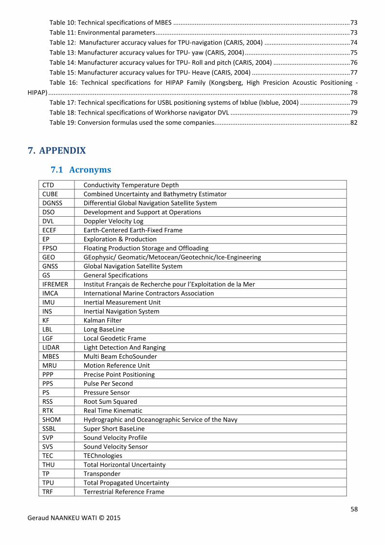
58 Geraud NAANKEU WATI © 2015
Table 10: Technical specifications of MBES ................................................................................................... 73
Table 11: Environmental parameters ............................................................................................................. 73
Table 12: Manufacturer accuracy values for TPU‐navigation (CARIS, 2004) ................................................ 74
Table 13: Manufacturer accuracy values for TPU‐ yaw (CARIS, 2004) ........................................................... 75
Table 14: Manufacturer accuracy values for TPU‐ Roll and pitch (CARIS, 2004) ........................................... 76
Table 15: Manufacturer accuracy values for TPU‐ Heave (CARIS, 2004) ....................................................... 77
Table 16: Technical specifications for HIPAP Family (Kongsberg, High Presicion Acoustic Positioning ‐
HIPAP) ......................................................................................................................................................................... 78
Table 17: Technical specifications for USBL positioning systems of Ixblue (Ixblue, 2004) ............................ 79
Table 18: Technical specifications of Workhorse navigator DVL ................................................................... 79
Table 19: Conversion formulas used the some companies............................................................................ 82
7. APPENDIX
7.1 Acronyms
CTD Conductivity Temperature Depth
CUBE Combined Uncertainty and Bathymetry Estimator
DGNSS Differential Global Navigation Satellite System
DSO Development and Support at Operations
DVL Doppler Velocity Log
ECEF Earth‐Centered Earth‐Fixed Frame
EP Exploration & Production
FPSO Floating Production Storage and Offloading
GEO GEophysic/ Geomatic/Metocean/Geotechnic/Ice‐Engineering
GNSS Global Navigation Satellite System
GS General Specifications
IFREMER Institut Français de Recherche pour l’Exploitation de la Mer
IMCA International Marine Contractors Association
IMU Inertial Measurement Unit
INS Inertial Navigation System
KF Kalman Filter
LBL Long BaseLine
LGF Local Geodetic Frame
LIDAR Light Detection And Ranging
MBES Multi Beam EchoSounder
MRU Motion Reference Unit
PPP Precise Point Positioning
PPS Pulse Per Second
PS Pressure Sensor
RSS Root Sum Squared
RTK Real Time Kinematic
SHOM Hydrographic and Oceanographic Service of the Navy
SSBL Super Short BaseLine
SVP Sound Velocity Profile
SVS Sound Velocity Sensor
TEC TEChnologies
THU Total Horizontal Uncertainty
TP Transponder
TPU Total Propagated Uncertainty
TRF Terrestrial Reference Frame
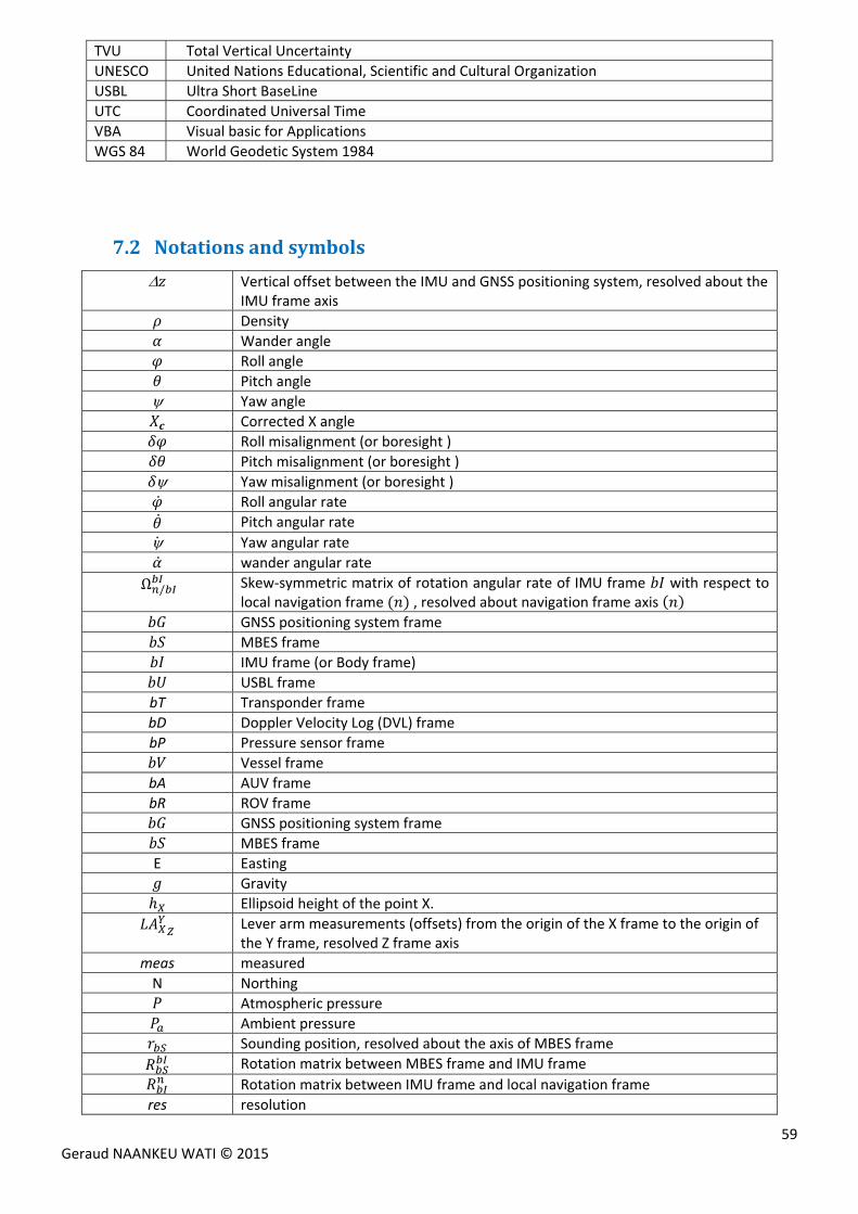
59 Geraud NAANKEU WATI © 2015
TVU Total Vertical Uncertainty
UNESCO United Nations Educational, Scientific and Cultural Organization
USBL Ultra Short BaseLine
UTC Coordinated Universal Time
VBA Visual basic for Applications
WGS 84 World Geodetic System 1984
7.2 Notationsandsymbols
Vertical offset between the IMU and GNSS positioning system, resolved about the IMU frame axis
Density
Wander angle
Roll angle
Pitch angle
Yaw angle
Corrected X angle
Roll misalignment (or boresight )
Pitch misalignment (or boresight )
Yaw misalignment (or boresight )
Roll angular rate
Pitch angular rate
Yaw angular rate
wander angular rate
Ω / Skew‐symmetric matrix of rotation angular rate of IMU frame with respect to local navigation frame , resolved about navigation frame axis
GNSS positioning system frame
MBES frame
IMU frame (or Body frame)
USBL frame
bT Transponder frame
bD Doppler Velocity Log (DVL) frame
bP Pressure sensor frame
Vessel frame
bA AUV frame
bR ROV frame
GNSS positioning system frame
MBES frame
E Easting
Gravity
Ellipsoid height of the point X.
Lever arm measurements (offsets) from the origin of the X frame to the origin of the Y frame, resolved Z frame axis
meas measured
N Northing
Atmospheric pressure
Ambient pressure
Sounding position, resolved about the axis of MBES frame
Rotation matrix between MBES frame and IMU frame
Rotation matrix between IMU frame and local navigation frame
res resolution
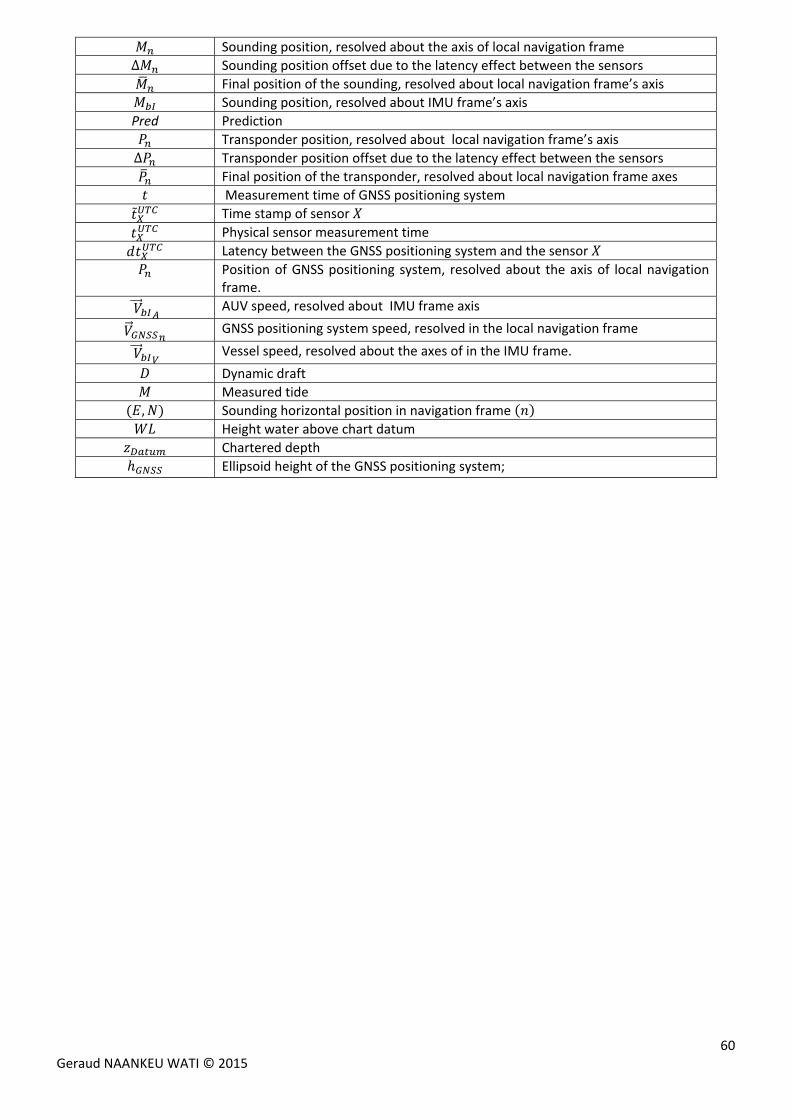
60 Geraud NAANKEU WATI © 2015
Sounding position, resolved about the axis of local navigation frame
∆ Sounding position offset due to the latency effect between the sensors
Final position of the sounding, resolved about local navigation frame’s axis
Sounding position, resolved about IMU frame’s axis
Pred Prediction
Transponder position, resolved about local navigation frame’s axis
∆ Transponder position offset due to the latency effect between the sensors
Final position of the transponder, resolved about local navigation frame axes
Measurement time of GNSS positioning system Time stamp of sensor
Physical sensor measurement time
Latency between the GNSS positioning system and the sensor
Position of GNSS positioning system, resolved about the axis of local navigation frame.
AUV speed, resolved about IMU frame axis
GNSS positioning system speed, resolved in the local navigation frame
Vessel speed, resolved about the axes of in the IMU frame.
Dynamic draft
Measured tide
, Sounding horizontal position in navigation frame
Height water above chart datum
Chartered depth
Ellipsoid height of the GNSS positioning system;
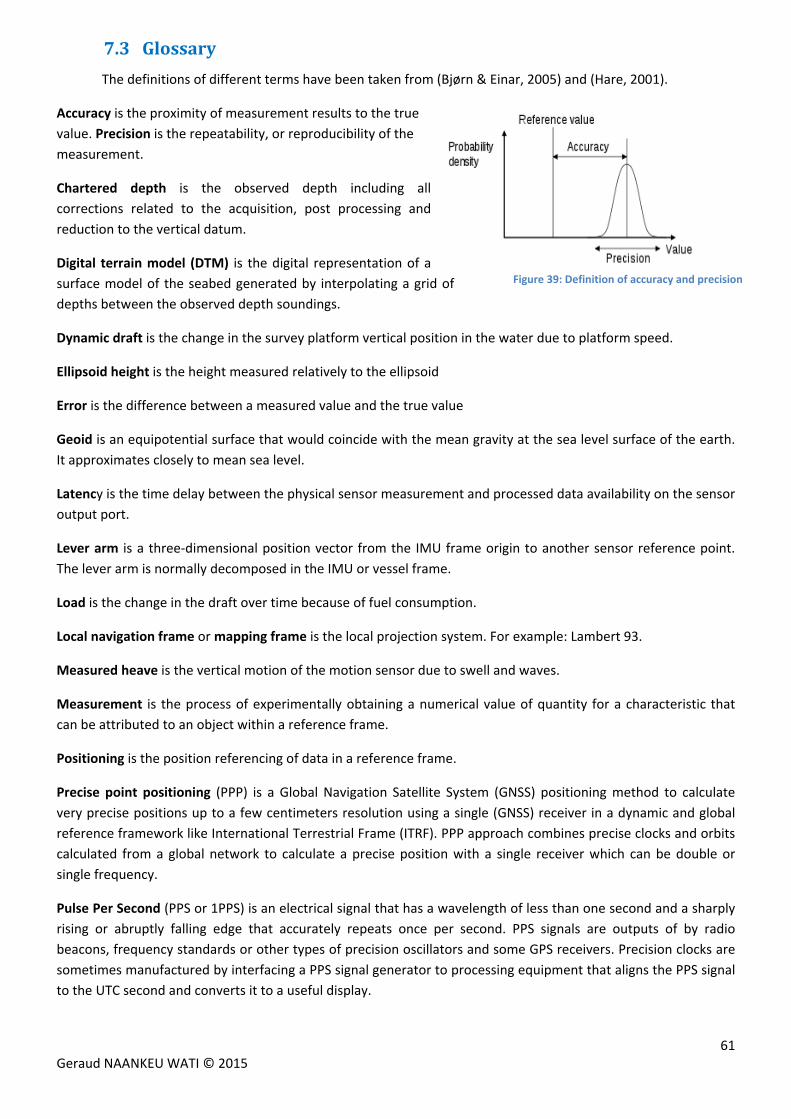
61 Geraud NAANKEU WATI © 2015
7.3 Glossary
The definitions of different terms have been taken from (Bjørn & Einar, 2005) and (Hare, 2001).
Accuracy is the proximity of measurement results to the true
value. Precision is the repeatability, or reproducibility of the
measurement.
Chartered depth is the observed depth including all
corrections related to the acquisition, post processing and
reduction to the vertical datum.
Digital terrain model (DTM) is the digital representation of a
surface model of the seabed generated by interpolating a grid of
depths between the observed depth soundings.
Dynamic draft is the change in the survey platform vertical position in the water due to platform speed.
Ellipsoid height is the height measured relatively to the ellipsoid
Error is the difference between a measured value and the true value
Geoid is an equipotential surface that would coincide with the mean gravity at the sea level surface of the earth.
It approximates closely to mean sea level.
Latency is the time delay between the physical sensor measurement and processed data availability on the sensor
output port.
Lever arm is a three‐dimensional position vector from the IMU frame origin to another sensor reference point.
The lever arm is normally decomposed in the IMU or vessel frame.
Load is the change in the draft over time because of fuel consumption.
Local navigation frame or mapping frame is the local projection system. For example: Lambert 93.
Measured heave is the vertical motion of the motion sensor due to swell and waves.
Measurement is the process of experimentally obtaining a numerical value of quantity for a characteristic that
can be attributed to an object within a reference frame.
Positioning is the position referencing of data in a reference frame.
Precise point positioning (PPP) is a Global Navigation Satellite System (GNSS) positioning method to calculate
very precise positions up to a few centimeters resolution using a single (GNSS) receiver in a dynamic and global
reference framework like International Terrestrial Frame (ITRF). PPP approach combines precise clocks and orbits
calculated from a global network to calculate a precise position with a single receiver which can be double or
single frequency.
Pulse Per Second (PPS or 1PPS) is an electrical signal that has a wavelength of less than one second and a sharply
rising or abruptly falling edge that accurately repeats once per second. PPS signals are outputs of by radio
beacons, frequency standards or other types of precision oscillators and some GPS receivers. Precision clocks are
sometimes manufactured by interfacing a PPS signal generator to processing equipment that aligns the PPS signal
to the UTC second and converts it to a useful display.
Figure 39: Definition of accuracy and precision
62 Geraud NAANKEU WATI © 2015
Random errors are errors in measurement that lead to measurable values being inconsistent when repeated
measures of a constant attribute or quantity are taken.
Real‐time, a real‐time system responds in a (timely) predictable way to unpredictable external stimuli arrivals. In
the context of this document; a processor responsible for time stamping reacts within a given predictable time
interval when a measurement arrives.
Sensor is an instrument that reacts to certain physical conditions and provides information (measurement) on
these.
Squat is the variation of the draft due to the changes of the vessel speed.
System is the integration of two or more sensors.
Systematic error is a type of error that deviates by a fixed amount from the true value of measurement. A
systematic error may also be an error having a nonzero mean, so that its effect is not reduced when observations
are averaged.
Time stamp is the time at which a data is recorded by taking into account the computation time in the system.
Total horizontal uncertainty (THU) is the component of total propagated uncertainty (TPU) calculated in the
horizontal plane.
Total propagated uncertainty (TPU) is the result of uncertainty propagation, when all contributing measurement
uncertainties, both random and systematic, have been included in the propagation. Uncertainty propagation
combines the effects of measurement uncertainties from several sources upon the uncertainties of derived or
calculated parameters.
Total vertical uncertainty (TVU) is the component of total propagated uncertainty (TPU) calculated in the vertical
dimension. TVU is a 1 Dimensional quantity.
True measurement time is the time at which a data is measured.
Uncertainty is the interval (for a given value) that will contain the true value of measurements at a specific
confidence level. The confidence level of the interval and the assumed statistical distribution of errors must also
be quoted. In the context of the standard of International Hydrographic Organization (OHI) the terms uncertainty
and confidence interval are equivalent.
7.4 Identificationofuncertaintysourcesforhydrographicsystems
Both tables below Table 8 and Table 9 present modern processes and practices that can help the
hydrographic surveyors provide more realistic uncertainty estimates or help minimize influential components that
are difficult to measure or model. This work has been done by Jason Bartlett and Rob hare. For more information
about the computation of various uncertainty sources, see (Jason & Rob, 2011).
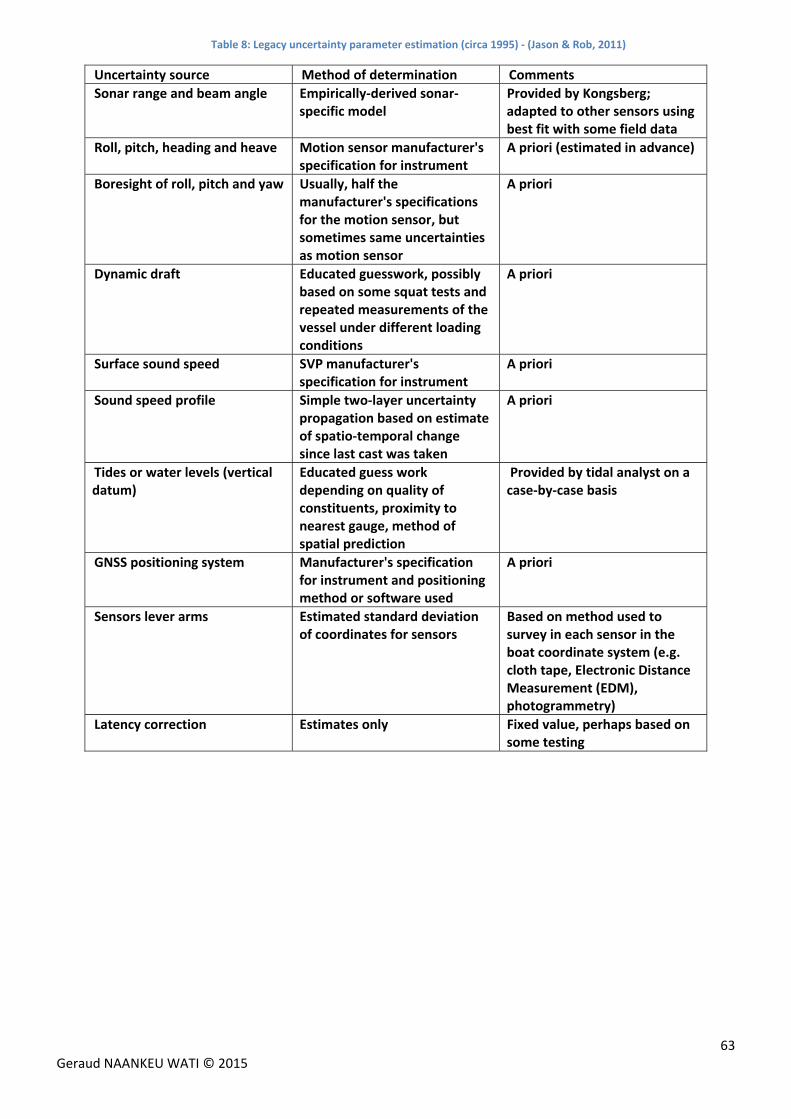
63 Geraud NAANKEU WATI © 2015
Table 8: Legacy uncertainty parameter estimation (circa 1995) ‐ (Jason & Rob, 2011)
Uncertainty source Method of determination Comments
Sonar range and beam angle Empirically‐derived sonar‐specific model
Provided by Kongsberg; adapted to other sensors using best fit with some field data
Roll, pitch, heading and heave Motion sensor manufacturer's specification for instrument
A priori (estimated in advance)
Boresight of roll, pitch and yaw Usually, half the manufacturer's specifications for the motion sensor, but sometimes same uncertainties as motion sensor
A priori
Dynamic draft Educated guesswork, possibly based on some squat tests and repeated measurements of the vessel under different loading conditions
A priori
Surface sound speed SVP manufacturer's specification for instrument
A priori
Sound speed profile Simple two‐layer uncertainty propagation based on estimate of spatio‐temporal change since last cast was taken
A priori
Tides or water levels (vertical datum)
Educated guess work depending on quality of constituents, proximity to nearest gauge, method of spatial prediction
Provided by tidal analyst on a case‐by‐case basis
GNSS positioning system Manufacturer's specification for instrument and positioning method or software used
A priori
Sensors lever arms Estimated standard deviation of coordinates for sensors
Based on method used to survey in each sensor in the boat coordinate system (e.g. cloth tape, Electronic Distance Measurement (EDM), photogrammetry)
Latency correction Estimates only Fixed value, perhaps based on some testing
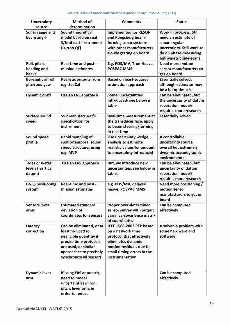
64 Geraud NAANKEU WATI © 2015
Table 9: Status of uncertainty source estimation today‐ (Jason & Rob, 2011)
Uncertainty source
Method of determination
Comments Status
Sonar range and beam angle
Sound theoretical model based on real S/N of each instrument (Lurton QF)
Implemented for RESON and Kongsberg beam‐forming sonar systems, with other manufacturers slowly getting on board
Work in progress. Still need an estimate of sonar angular uncertainty. Still work to do on phase‐measuring bathymetric side‐scans
Roll, pitch, heading and heave
Real‐time and post‐mission estimates
E.g. POS/MV, True‐Heave, POSPAC MMS
Need more motion sensor manufacturers to get on board
Boresight of roll, pitch and yaw
Realistic outputs from e.g. SeaCal
Based on least‐squares estimation approach
Essentially solved, although estimates may be a bit optimistic
Dynamic draft Use an ERS approach Some uncertainties introduced‐ see below in table
Can be eliminated, but the uncertainty of datum separation models requires more research
Surface sound speed
SVP manufacturer's specification for instrument
Real‐time measurement at the transducer face, apply to beam steering/forming in real‐time
Essentially solved
Sound speed profile
Rapid sampling of spatio‐temporal sound speed structure, using e.g. MVP
Use uncertainty wedge analysis to estimate realistic values for amount to uncertainty introduced
A controllable uncertainty source overall but extremely dynamic oceanographic environments
Tides or water levels ( vertical datum)
Use an ERS approach But, we introduce new uncertainties, see below in table.
Can be eliminated, but uncertainty of datum separation models requires more research
GNSS positioning system
Real‐time and post‐mission estimates
e.g. POS/MV, delayed heave, POSPAC MMS
Need more positioning / motion sensor manufacturers to get on board
Sensors lever arms
Estimated standard deviation of coordinates for sensors
Proper over‐determined sensor survey with output variance‐covariance matrix of coordinates
Can be computed effectively
Latency correction
Can be eliminated, or at least reduced to negligible quantitiy if precise time protocols are used, or similar approaches to precisely synchronize all sensors
IEEE 1588‐2002 PTP based on a network time protocol that effectively eliminates dynamic motion residuals due to small timing errors in the instrumentation.
A solvable problem with some hardware and software
Dynamic lever arm
If using ERS approach, need to model uncertainties in roll, pitch, lever arm, in order to reduce
Can be computed effectively
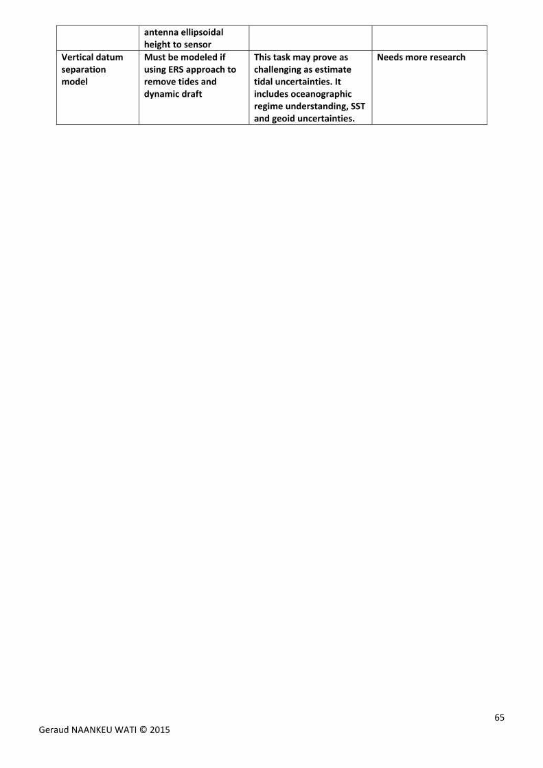
65 Geraud NAANKEU WATI © 2015
antenna ellipsoidal height to sensor
Vertical datum separation model
Must be modeled if using ERS approach to remove tides and dynamic draft
This task may prove as challenging as estimate tidal uncertainties. It includes oceanographic regime understanding, SST and geoid uncertainties.
Needs more research
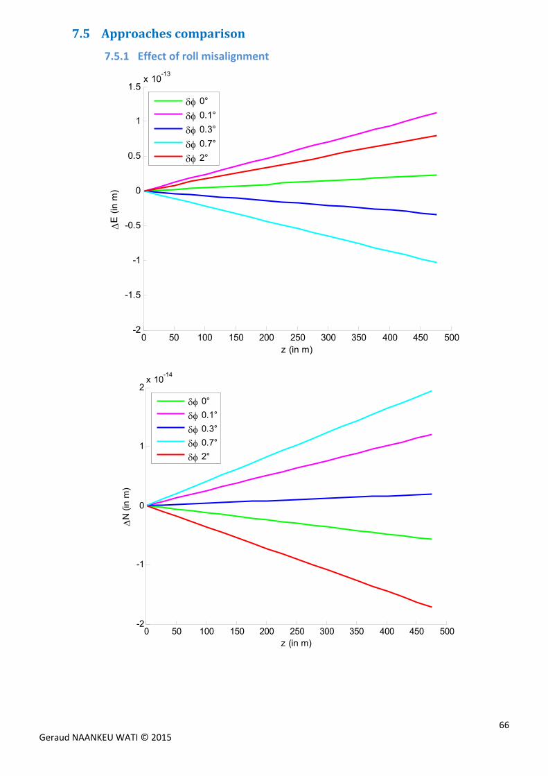
66 Geraud NAANKEU WATI © 2015
7.5 Approachescomparison
7.5.1 Effect of roll misalignment
0 50 100 150 200 250 300 350 400 450 500-2
-1.5
-1
-0.5
0
0.5
1
1.5x 10
-13
z (in m)
E
(in
m)
0°
0.1°
0.3°
0.7°
2°
0 50 100 150 200 250 300 350 400 450 500-2
-1
0
1
2x 10
-14
z (in m)
N
(in
m)
0°
0.1°
0.3°
0.7°
2°
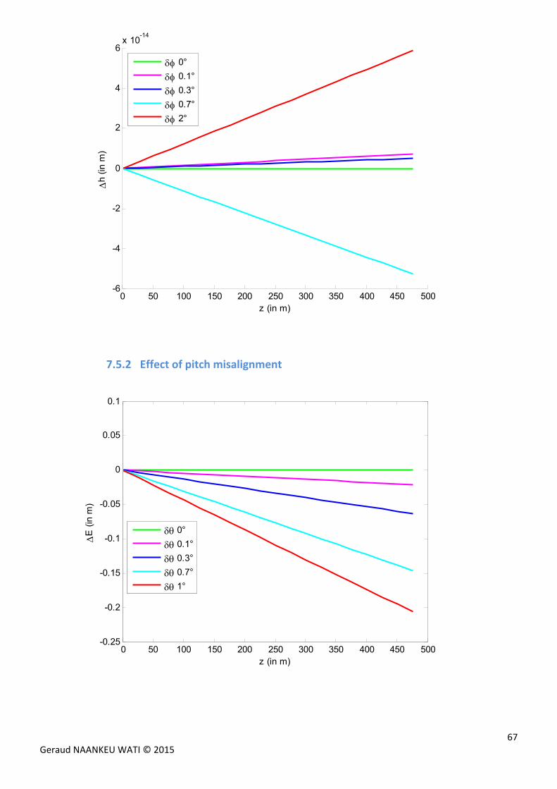
67 Geraud NAANKEU WATI © 2015
7.5.2 Effect of pitch misalignment
0 50 100 150 200 250 300 350 400 450 500-6
-4
-2
0
2
4
6x 10
-14
z (in m)
h
(in m
)
0°
0.1°
0.3°
0.7°
2°
0 50 100 150 200 250 300 350 400 450 500-0.25
-0.2
-0.15
-0.1
-0.05
0
0.05
0.1
z (in m)
E
(in
m)
0°
0.1°
0.3°
0.7°
1°
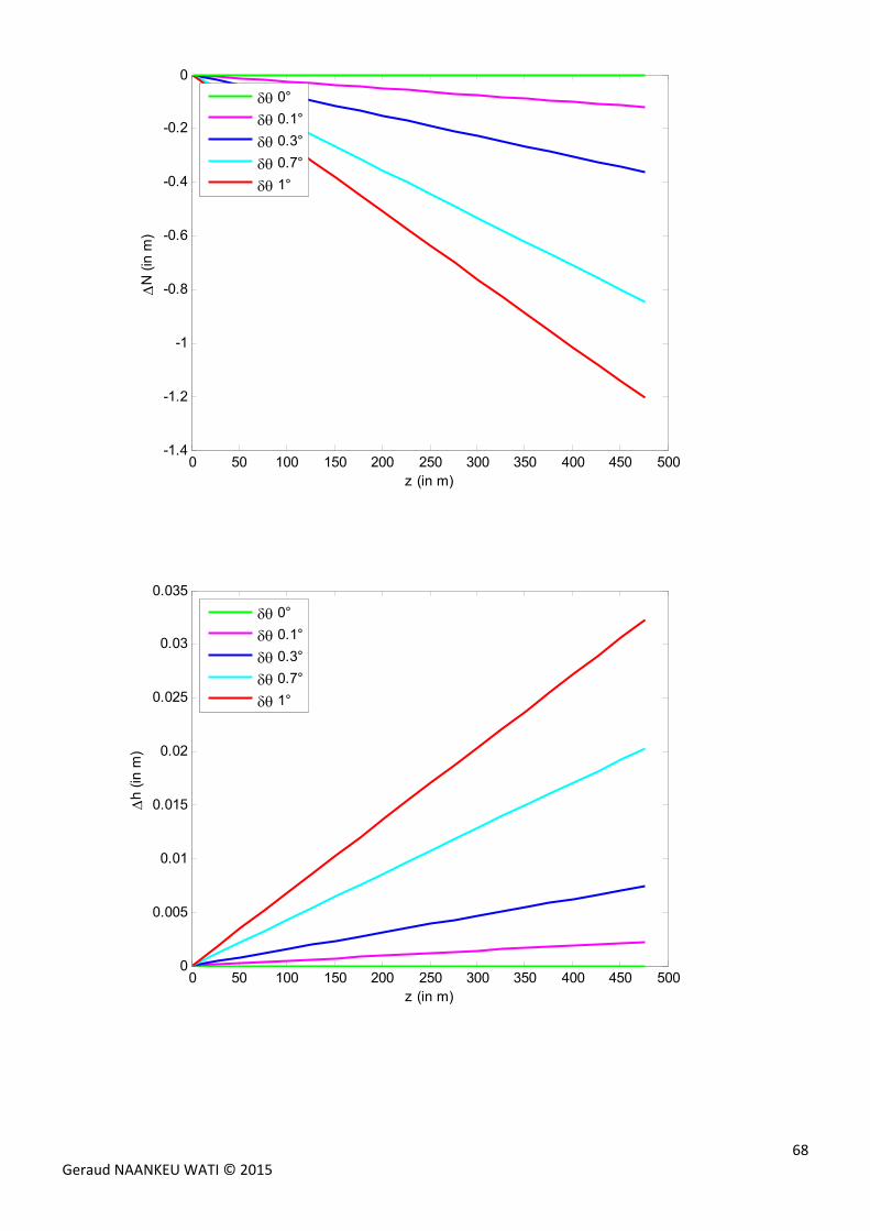
68 Geraud NAANKEU WATI © 2015
0 50 100 150 200 250 300 350 400 450 500-1.4
-1.2
-1
-0.8
-0.6
-0.4
-0.2
0
z (in m)
N
(in
m)
0°
0.1°
0.3°
0.7°
1°
0 50 100 150 200 250 300 350 400 450 5000
0.005
0.01
0.015
0.02
0.025
0.03
0.035
z (in m)
h
(in m
)
0°
0.1°
0.3°
0.7°
1°
69 Geraud NAANKEU WATI © 2015
7.6 Errormodelforhydrographicsurveysystems
7.6.1 Error model for a surface survey system
As summarized in the standard norms of the International Hydrographic Organization (Internationale
Organisation Hydrographique, 2011) and the work of (Debese, 2013), the errors associated with the evaluation of
the horizontal position of a single beam for a surface survey system must include:
Errors of GNSS positioning system measurement ;
Error of measurement of slant range and incidence angles by the MBES;
Error of the sound speed measurement, including the measurement errors of sound velocity profile and
the extrapolation of sound velocity profile;
Error of misalignment angles measurement between the sensors;
Errors of IMU measurement (roll, pitch and yaw);
Error of lever arms measurements ;
Error of latency measurement between sensors;
Error of vessel speed measurement.
Factors contributing to the uncertainty of sounding vertical position include:
Errors of GNSS positioning system measurement ;
Error of measurement of slant range and incidence angles by the MBES;
Error of tide measurement;
Error of speed of sound measurement, including the measurement errors of sound velocity profile and
the extrapolation of sound velocity profile;
Error of misalignment angles measurement between the sensors;
Error of lever arms measurement ;
Error of the vertical datum separation model;
Error of latency measurement between sensors.
Errors related to the motion of the vessel (roll, pitch, yaw (slope) and heave);
Error of dynamic draft measurement;
Seabed slope;
Error of vessel speed measurement.
According to (Debese, 2013) the most important error sources are the following: the measurement errors
of sound speed, heave, tide, latency, yaw and pitch.
7.6.2 Error model for an underwater survey system
In an underwater survey system, the various error sources which contribute to the horizontal uncertainty of
a sounding must include:
Errors of GNSS positioning system measurement ;
Error of measurement of slant range and incidence angles by the MBES;
Error of measurement of slant range and incidence angles by the USBL;
Error of the sound speed measurement, including the measurement errors of sound velocity profile, the
extrapolation of sound velocity profile;
Error of misalignment angles measurement between the sensors;
Errors of motion sensors measurement (roll, pitch and yaw);
Error of lever arms measurement ;
Error of latency measurement between sensors;
Error of horizontal position measurement of Doppler Velocity Log (DVL);
70 Geraud NAANKEU WATI © 2015
Error of vessel speed measurement.
Factors contributing to the vertical uncertainty of a sounding must include:
Errors of GNSS positioning system measurement ;
Error of measurement of slant range and incidence angles by the MBES;
Error of measurement of slant range and incidence angles by the USBL;
Error of misalignment angles measurement between the sensors;
Error of tide measurement;
Error of speed of sound measurement;
Error of lever arms measurement ;
Error of the vertical datum separation model;
Error of latency measurement between sensors;
Errors related to the motion of the vessel and the underwater vehicle(roll, pitch, yaw and heave);
Error of dynamic draft measurement;
Error of barometer and pressure sensor pressure measurement;
Error of water density measurement;
Error of gravity measurement;
Seabed slope;
Error of vessel speed measurement.
7.6.3 Difference between random and systematic errors
The differences between a systematic error and a random error can be illustrated using a target and arrows
image: the target center (in green) represents the quantity to be measured and each point in black is a
measurement of this quantity. The mean value of the measured quantities is represented in blue.
Figure 40 : Difference between random and systematic errors‐ (Exell, 2001)‐[modified]
Note that the systematic and random errors refer to problems associated with data acquisition. Mistakes
occurring in the calculations or when reading the instrument are not considered in the error budget analysis
7.7 Rotationmatrixesbetweentwoframes
7.7.1 Rotation matrix from LGF to TRF
The rotation matrix from the LGF to the TRF can be achieved by two rotations:
1. A rotation around the local East axis by the angle . It can be represented by the following matrix.
High accuracy High precision
Low accuracy High precision
High accuracy Low precision
Low accuracy Low precision
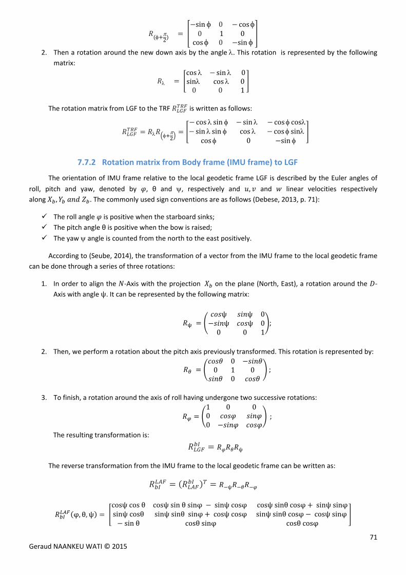
71 Geraud NAANKEU WATI © 2015
2
sin 0 cos0 1 0
cos 0 sin
2. Then a rotation around the new down axis by the angle. This rotation is represented by the following matrix:
cos sin 0sin cos 00 0 1
The rotation matrix from LGF to the TRF is written as follows:
cos sin sin cos cossin sin cos cos sincos 0 sin
7.7.2 Rotation matrix from Body frame (IMU frame) to LGF
The orientation of IMU frame relative to the local geodetic frame LGF is described by the Euler angles of
roll, pitch and yaw, denoted by , θ and , respectively and , and linear velocities respectively
along , . The commonly used sign conventions are as follows (Debese, 2013, p. 71):
The roll angle is positive when the starboard sinks;
The pitch angle θ is positive when the bow is raised;
The yaw angle is counted from the north to the east positively.
According to (Seube, 2014), the transformation of a vector from the IMU frame to the local geodetic frame
can be done through a series of three rotations:
1. In order to align the ‐Axis with the projection on the plane (North, East), a rotation around the ‐
Axis with angleψ. It can be represented by the following matrix:
ψ ψ 0ψ ψ 0
0 0 1;
2. Then, we perform a rotation about the pitch axis previously transformed. This rotation is represented by:
0
0 1 00
;
3. To finish, a rotation around the axis of roll having undergone two successive rotations:
1 0 000
;
The resulting transformation is:
ψ
The reverse transformation from the IMU frame to the local geodetic frame can be written as:
ψ
φ, θ, ψ cosψcosθ cosψsinθsinφ sinψcosφ cosψsinθcosφ sinψsinφsinψcosθ sinψsinθsinφ cosψcosφ sinψsinθcosφ cosψsinφ
sinθ cosθsinφ cosθcosφ
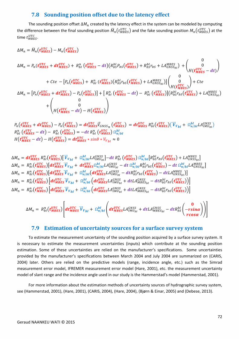
72 Geraud NAANKEU WATI © 2015
7.8 Soundingpositionoffsetduetothelatencyeffect
The sounding position offset ∆ created by the latency effect in the system can be modeled by computing
the difference between the final sounding position and the fake sounding position at the
time .
∆
∆ 00
00
∆
00
Ω /
Ω /
∗ ∗ 0
∆ Ω / Ω /
∆ Ω / Ω / Ω /
∆ Ω /
∆ Ω /
∆ Ω /
∆ Ω /
7.9 Estimationofuncertaintysourcesforasurfacesurveysystem
To estimate the measurement uncertainty of the sounding position acquired by a surface survey system. It
is necessary to estimate the measurement uncertainties (inputs) which contribute at the sounding position
estimation. Some of these uncertainties are relied on the manufacturer’s specifications. Some uncertainties
provided by the manufacturer’s specifications between March 2004 and July 2004 are summarized on (CARIS,
2004) later. Others are relied on the predictive models (range, incidence angle, etc.) such as the Simrad
measurement error model, IFREMER measurement error model (Hare, 2001), etc. the measurement uncertainty
model of slant range and the incidence angle used in our study is the Hammerstad’s model (Hammerstad, 2001).
For more information about the estimation methods of uncertainty sources of hydrographic survey system,
see (Hammerstad, 2001), (Hare, 2001), (CARIS, 2004), (Hare, 2004), (Bjørn & Einar, 2005) and (Debese, 2013).
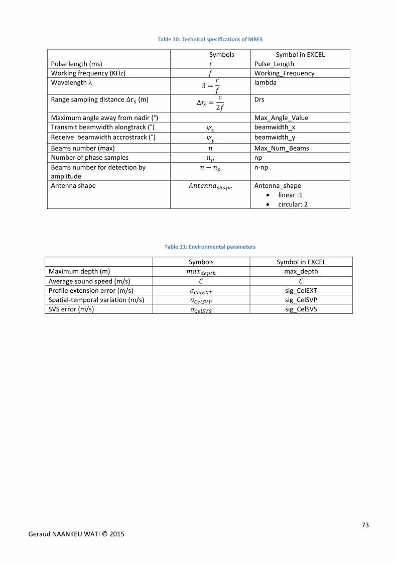
73 Geraud NAANKEU WATI © 2015
Table 10: Technical specifications of MBES
Symbols Symbol in EXCELPulse length (ms) Pulse_Length
Working frequency (KHz) Working_Frequency
Wavelength lambda
Range sampling distance ∆r (m)
∆2 Drs
Maximum angle away from nadir (°) Max_Angle_Value
Transmit beamwidth alongtrack (°) beamwidth_x
Receive beamwidth accrostrack (°) beamwidth_y
Beams number (max) Max_Num_Beams
Number of phase samples np
Beams number for detection by amplitude
n‐np
Antenna shape
Antenna_shape
linear :1
circular: 2
Table 11: Environmental parameters
Symbols Symbol in EXCEL
Maximum depth (m) max_depth
Average sound speed (m/s)
Profile extension error (m/s) sig_CelEXT
Spatial‐temporal variation (m/s) sig_CelSVP
SVS error (m/s) sig_CelSVS
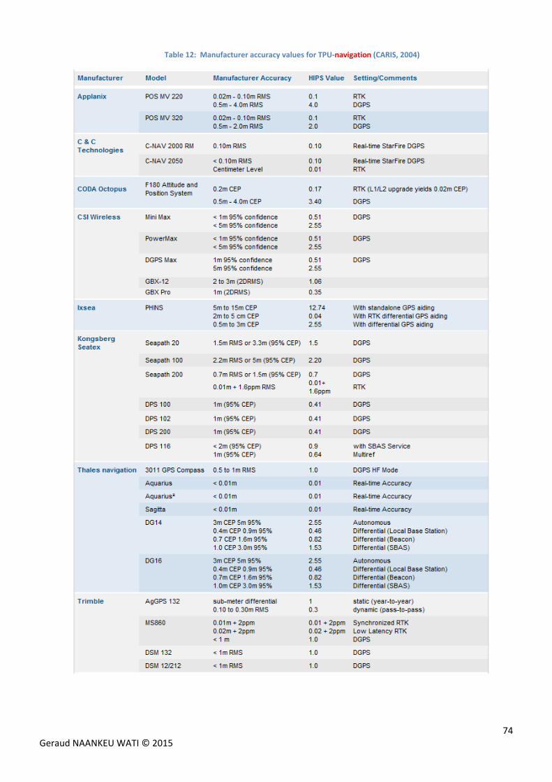
74 Geraud NAANKEU WATI © 2015
Table 12: Manufacturer accuracy values for TPU‐navigation (CARIS, 2004)
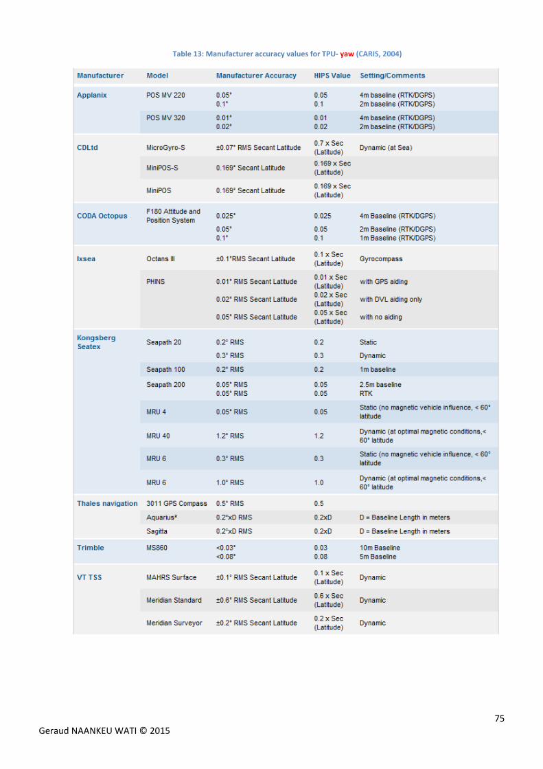
75 Geraud NAANKEU WATI © 2015
Table 13: Manufacturer accuracy values for TPU‐ yaw (CARIS, 2004)
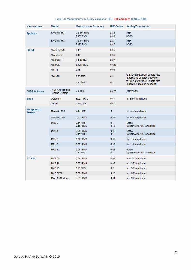
76 Geraud NAANKEU WATI © 2015
Table 14: Manufacturer accuracy values for TPU‐ Roll and pitch (CARIS, 2004)
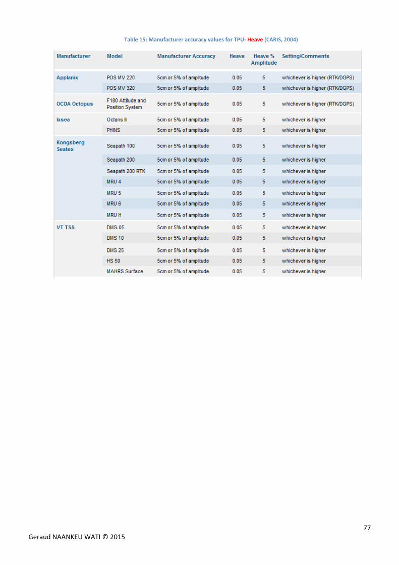
77 Geraud NAANKEU WATI © 2015
Table 15: Manufacturer accuracy values for TPU‐ Heave (CARIS, 2004)
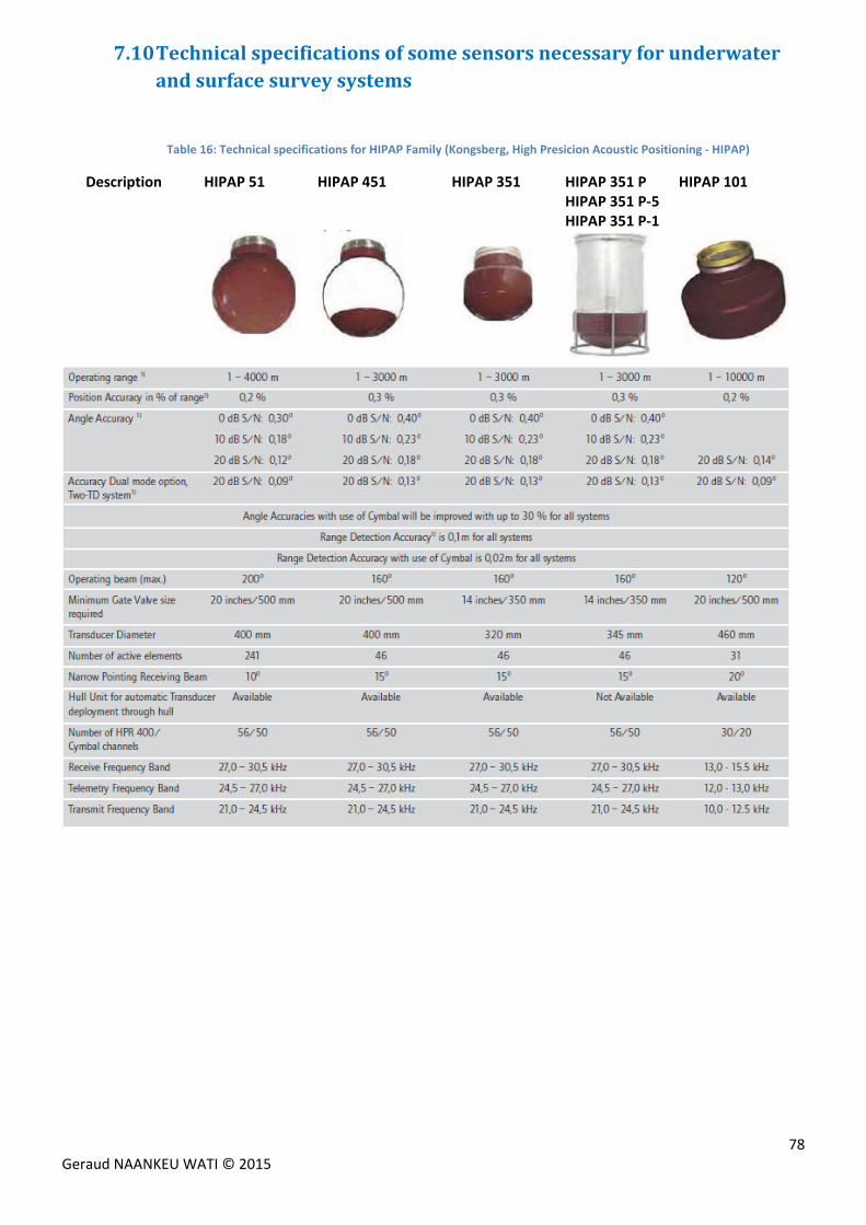
78 Geraud NAANKEU WATI © 2015
7.10 Technicalspecificationsofsomesensorsnecessaryforunderwaterandsurfacesurveysystems
Table 16: Technical specifications for HIPAP Family (Kongsberg, High Presicion Acoustic Positioning ‐ HIPAP)
Description HIPAP 51 HIPAP 451 HIPAP 351 HIPAP 351 P HIPAP 351 P‐5 HIPAP 351 P‐1
HIPAP 101
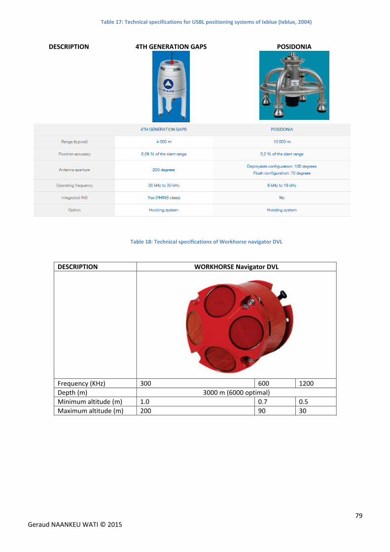
79 Geraud NAANKEU WATI © 2015
Table 17: Technical specifications for USBL positioning systems of Ixblue (Ixblue, 2004)
DESCRIPTION 4TH GENERATION GAPS POSIDONIA
Table 18: Technical specifications of Workhorse navigator DVL
DESCRIPTION WORKHORSE Navigator DVL
Frequency (KHz) 300 600 1200
Depth (m) 3000 m (6000 optimal)
Minimum altitude (m) 1.0 0.7 0.5
Maximum altitude (m) 200 90 30
80 Geraud NAANKEU WATI © 2015
7.11 Estimationofunderwatervehicleverticalposition
One of TOTAL main objectives is to better estimate the underwater vehicle vertical position relative to
chart datum in order to provide high resolution data for deepwater projects. The underwater vehicle vertical
position is traditionally estimated by combining the pressure sensor measurements with the density profile
estimate and measurements of tide and atmospheric pressure. However, the main challenge is due to the fact
that:
The density profile varies with position and time (the variation in depth is significant).
Gravitational acceleration depends on the vehicle’s position (latitude and the depth ).
Moreover, there are various formulas to estimate the underwater vehicle vertical position, commonly
called formulas from pressure to depth. These formulas used different computation algorithms of the sea water
properties (density, gravitational acceleration). Thus, it is useful these formulas and algorithms to find a good
solution of underwater vehicle vertical position estimate.
7.11.1 Computation algorithms of sea water properties
The sea water properties used to estimate the underwater vehicle vertical position are:
Salinity ;
Water density ;
Gravitational acceleration .
7.11.1.1 The salinity
The salinity , is directly related to conductivity15. It is estimated from the practical salinity scale
(PSS‐78) of Millero and Poisson below:
, ,, ,
35, 15, 0, ,
7.11.1.2 The density of the sea water
In the world of oil and gas industry, there are two algorithms for computation of the sea
waterdensity , / :
1. UNESCO formula , so‐called the international equation of state of sea water 1980 (IES‐80). It is
most used. It is function of the salinity , , the temperature , ° and the pressure ( , decibars).
It is given by:
, ,, , 0
1 / , ,
Where:
, , is the secant bulk modulus.
2. Formula used by Tritech International.
15The conductivity is the concentration of salt and other inorganic compounds in seawater.
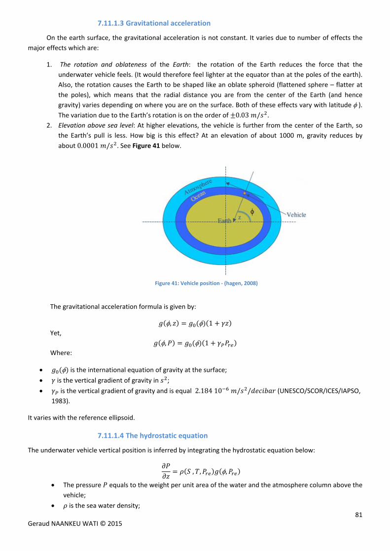
81 Geraud NAANKEU WATI © 2015
7.11.1.3 Gravitational acceleration
On the earth surface, the gravitational acceleration is not constant. It varies due to number of effects the
major effects which are:
1. The rotation and oblateness of the Earth: the rotation of the Earth reduces the force that the
underwater vehicle feels. (It would therefore feel lighter at the equator than at the poles of the earth).
Also, the rotation causes the Earth to be shaped like an oblate spheroid (flattened sphere – flatter at
the poles), which means that the radial distance you are from the center of the Earth (and hence
gravity) varies depending on where you are on the surface. Both of these effects vary with latitude). The variation due to the Earth’s rotation is on the order of 0.03 / .
2. Elevation above sea level: At higher elevations, the vehicle is further from the center of the Earth, so
the Earth’s pull is less. How big is this effect? At an elevation of about 1000 m, gravity reduces by
about0.0001 / . See Figure 41 below.
Figure 41: Vehicle position ‐ (hagen, 2008)
The gravitational acceleration formula is given by:
, 1
Yet,
, 1
Where:
is the international equation of gravity at the surface;
is the vertical gradient of gravity in ;
is the vertical gradient of gravity and is equal 2.18410 / / (UNESCO/SCOR/ICES/IAPSO,
1983).
It varies with the reference ellipsoid.
7.11.1.4 The hydrostatic equation
The underwater vehicle vertical position is inferred by integrating the hydrostatic equation below:
, , ,
The pressure equals to the weight per unit area of the water and the atmosphere column above the
vehicle;
is the sea water density;
82 Geraud NAANKEU WATI © 2015
is the gravitational acceleration.
For more details about the properties of the sea water, see (UNESCO/SCOR/ICES/IAPSO, 1983).
7.11.2 Analysis of the traditional formulas of conversion from pressure to depth
based on the hydrostatic equation
In the world of oil and gas industry, two conversion formulas from pressure to depth are usually used to
determine the underwater vehicle vertical position:
The UNESCO formula and;
An empirical formula (by assuming that the sea water density is constant in the water column).
But, the formula, the most used by TOTAL contractors during the acquisition campaigns is the empirical
formula. (See the Table 19 below).
Table 19: Conversion formulas used the some companies
Companies Formula of conversion from pressure to depth
Fugro Empirical formula /UNESCO formula
C&C Empirical formula/UNESCO formula
Norwegian Defence research establishment UNESCO formula
QINSy (from Norwegian Defence research establishment)
UNESCO formula
7.11.2.1 Analysis of the UNESCO formula
The UNESCO formula supposes that the sea water condition in the water column is equal to Standard
Ocean with temperature =0 °C, and salinity =35 PSU. A correction term is calculated to for the conditions
deviating from standard ocean (Temperature=0 °C, and salinity=35 PSU).
7.11.2.1.1 Algorithm of UNESCO formula
From the hydrostatic equation:
, , ,
, ,, ,
, 1
Where:
, , is the specific volume of water.
The pressure equals to the weight per unit area of the water and the atmosphere column above the
vehicle;
is the pressure reduced of the atmospheric pressure at the sea level.
is the sea water density;
is the international equation of gravity at surface.
The equation can be simplified as below:
83 Geraud NAANKEU WATI © 2015
1 , ,
, , 35, 0, 35, 0,
35, 0,
, , 35, 0, 0
Where :
∆ , , 35, 0,
, ,
1 35, 0, 0
∆
But, , then :
1 35, 0, 0
∆
35, 0, 0 1
∆ 1
35, 0, 0 1
∆9.8
35, 0, 0 1
∆ 9.8
16
Where:
∆ is called specific volume anomaly en / ;
is the vertical position of the underwater vehicle (m);
35, 0, 22 3 4.
With:
9.72659
2.2512
2.279
1.82
The coefficients of this equation are determined using the least squares method with a precision equivalent to
0.0002 m or better at 12000 decibars. The least squares formula eliminates the need for computing logarithms with
negligible loss of precision. The uncertainty of this formula is to 0.1 m over the pressure range 0‐10000 decibars
(UNESCO/SCOR/ICES/IAPSO, 1983).
The specific volume anomaly ∆ enables to improve the depth accuracy. It is calculated numerically using the
difference between the estimated from the measured CTD profile , , and the specific volume of the standard
16 ∆
9.8
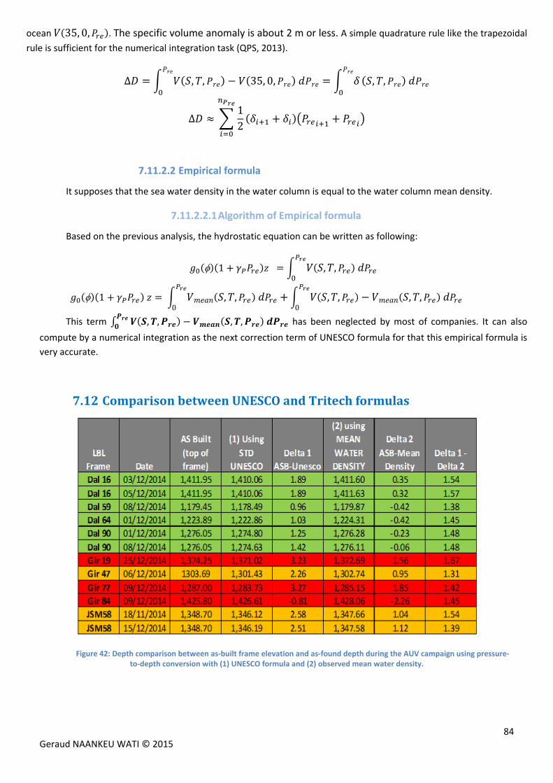
84 Geraud NAANKEU WATI © 2015
ocean 35, 0, . The specific volume anomaly is about 2 m or less. A simple quadrature rule like the trapezoidal
rule is sufficient for the numerical integration task (QPS, 2013).
∆ , , 35, 0,
, ,
∆12
7.11.2.2 Empirical formula
It supposes that the sea water density in the water column is equal to the water column mean density.
7.11.2.2.1 Algorithm of Empirical formula
Based on the previous analysis, the hydrostatic equation can be written as following:
1 , , 0
1 , , 0
, , , , 0
This term , , , , has been neglected by most of companies. It can also
compute by a numerical integration as the next correction term of UNESCO formula for that this empirical formula is
very accurate.
7.12 ComparisonbetweenUNESCOandTritechformulas
Figure 42: Depth comparison between as‐built frame elevation and as‐found depth during the AUV campaign using pressure‐to‐depth conversion with (1) UNESCO formula and (2) observed mean water density.
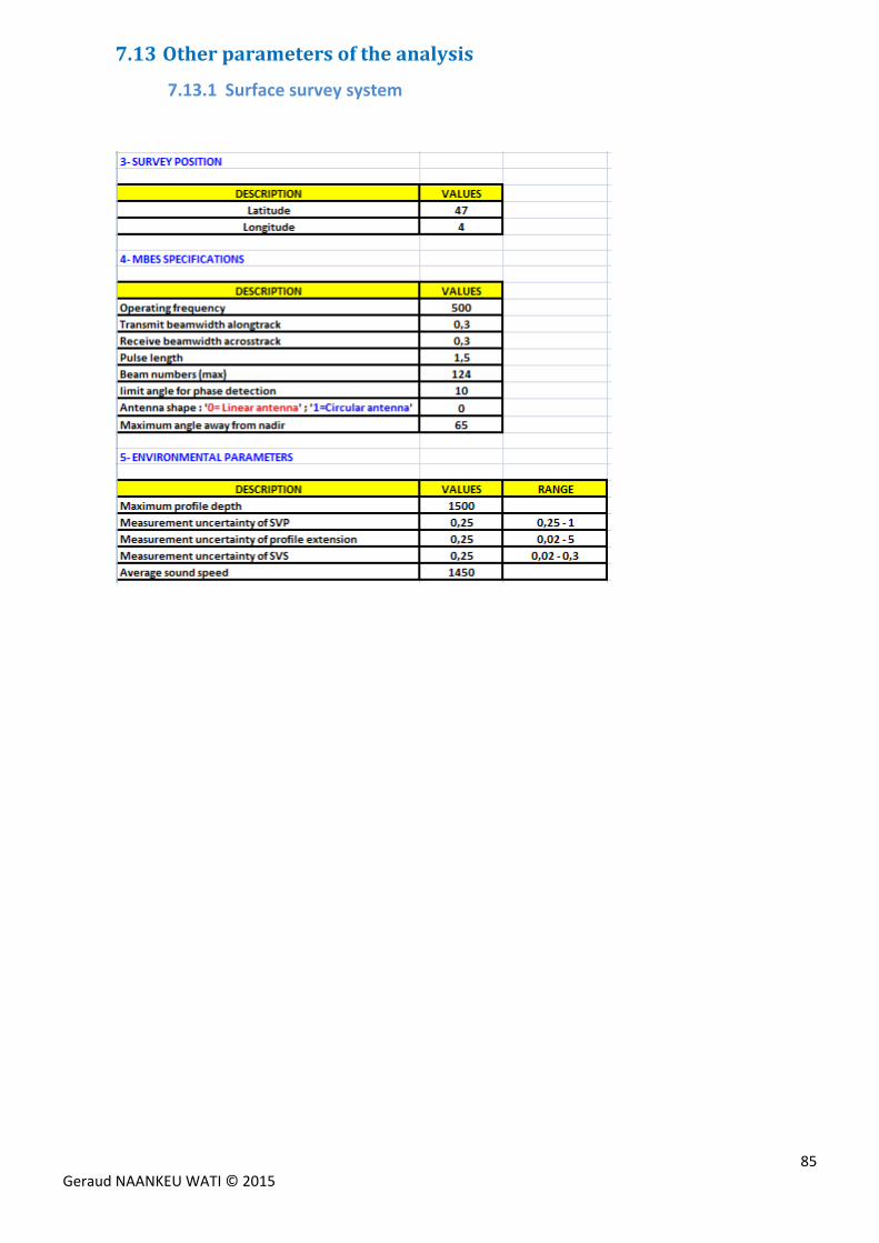
85 Geraud NAANKEU WATI © 2015
7.13 Otherparametersoftheanalysis
7.13.1 Surface survey system
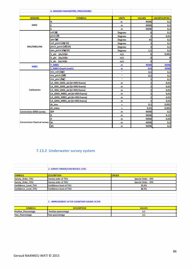
86 Geraud NAANKEU WATI © 2015
7.13.2 Underwater survey system
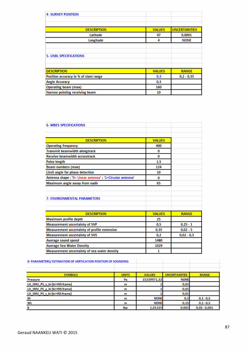
87 Geraud NAANKEU WATI © 2015
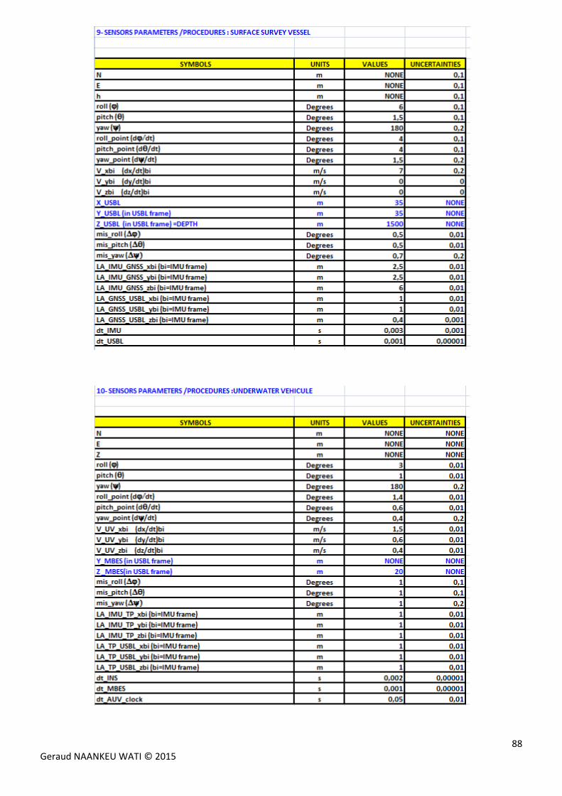
88 Geraud NAANKEU WATI © 2015
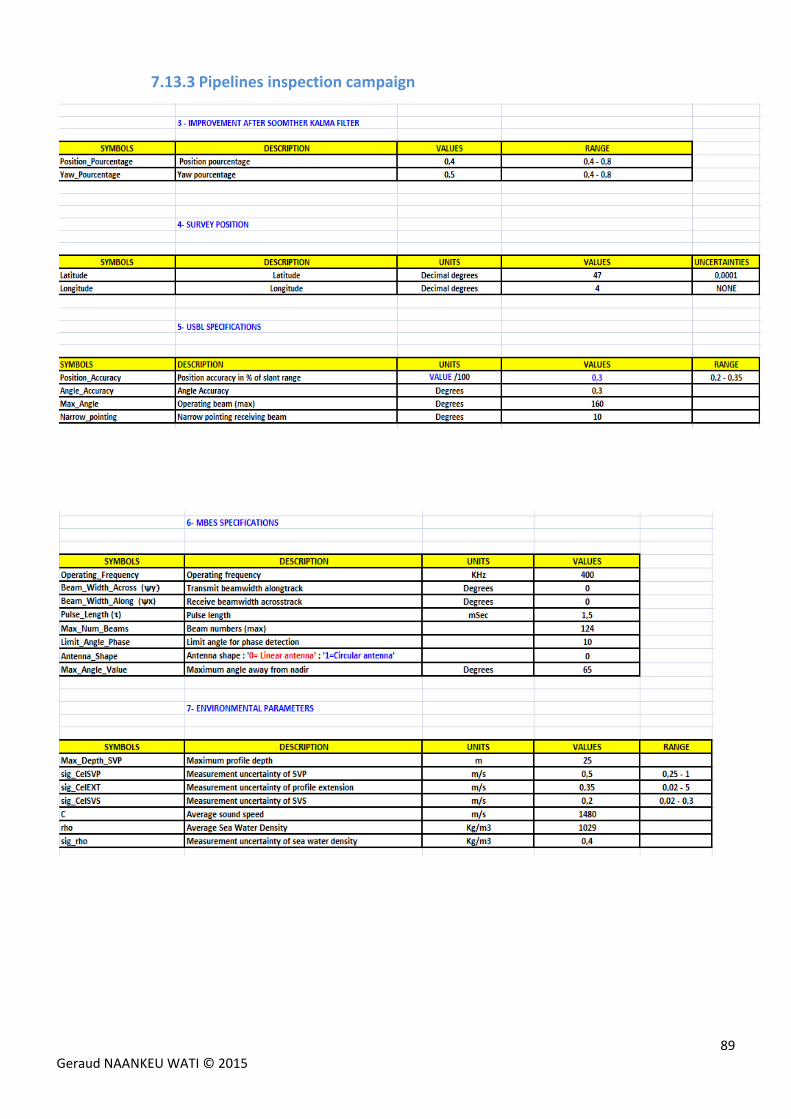
89 Geraud NAANKEU WATI © 2015
7.13.3 Pipelines inspection campaign
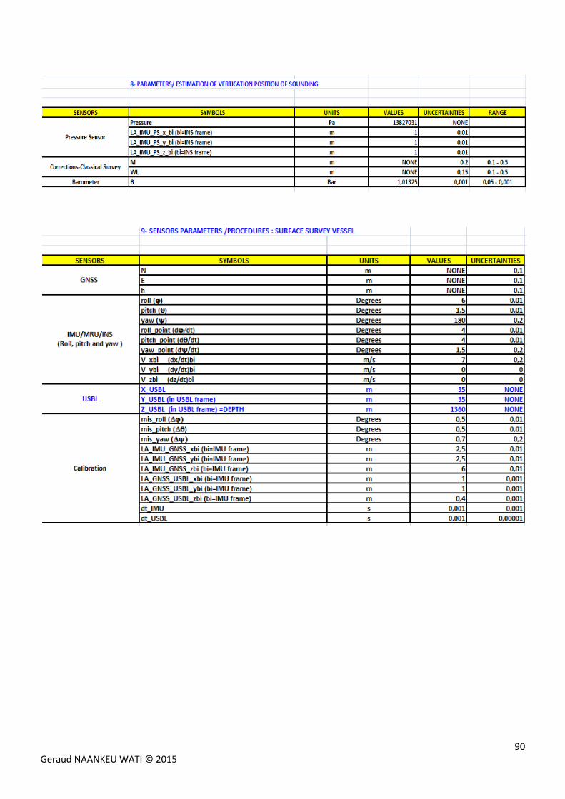
90 Geraud NAANKEU WATI © 2015
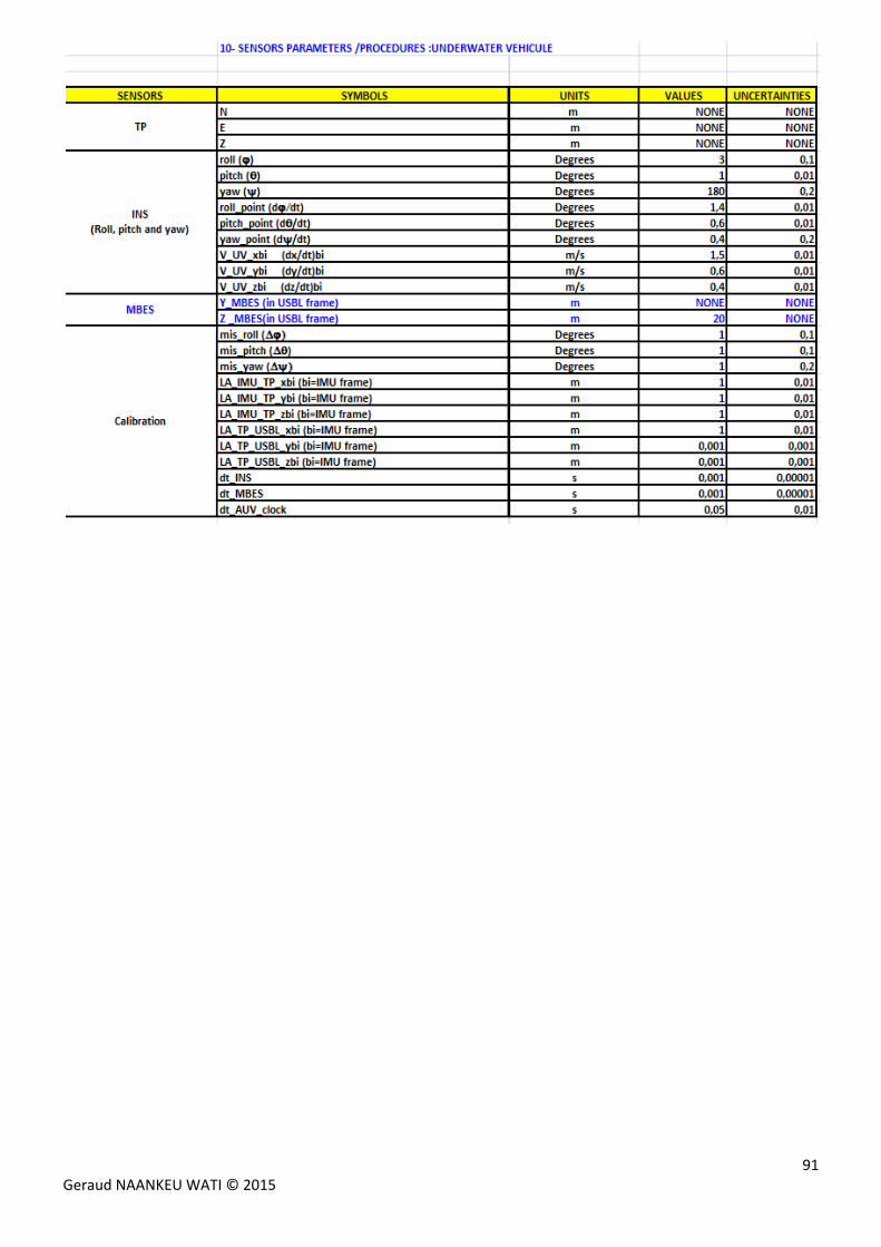
91 Geraud NAANKEU WATI © 2015

92 Geraud NAANKEU WATI © 2015
ENSTA BRETAGNE
Ecole Nationale Supérieure de Techniques Avancées Bretagne
Final Year Project in HydrographyAuthor: Geraud NAANKEU WATI Promotion 2015
Title: Error budget analysis for hydrographic survey systems; comparative study of methods and existing softwares; implementation on an inspection campaign of pipelines by AUV.
Thesis defence: 04 September 2015
Host institution TOTAL E&P
Volumes number: 1 Pages number: 50 (Report) +42 (Appendix)
Bibliographic references number: 78
Abstract
To install subsea infrastructures (pipelines, subsea wells, etc) necessary for the development of hydrocarbon resources, TOTAL regularly contracts hydrographic companies to perform hydrographic surveys. These companies mainly use two types of hydrographic survey systems: surface survey systems (generally used in near shore and in shallow water (0‐100 m)) and underwater survey systems (generally used in offshore and in deep offshore (100‐3000 m)). Each company has its own method to estimate the error budget of a hydrographic survey system. Their method is usually based on the law of uncertainty propagation (Hare, 2001). This work’s objective is to study and compare various methods of error budget estimation used by TOTAL contractors and other existing tools on the market, in order to better qualify the hydrographic data. The state of the art of classical error budget estimation methods of these systems and the analysis of their limits have allowed to propose an estimation method of error budget for the surface and underwater survey systems. This work also contributes to improving the sounding position acquired by underwater and surface survey systems, demonstrating the yaw misalignment influence between the inertial sensors (IMU, etc) and proximity sensor (MBES, etc) on sounding vertical position, stressing the importance of automatic calibration methods relative to the classical method of patch test and clarifying the issue on the methods of conversion from pressure to depth.
Key words: Error budget, Positioning, Law of uncertainty propagation, Surface survey system,
Underwater survey system, Total Propagated Uncertainty, Multi Beam Echo Sounder, Underwater Vehicle.
![WELCOME []projects over the year. Here are Stephanie’s learning experiences and encouragements for future students. “Throughout my research assistantship experiences I have gained](https://img.pdfslide.net/doc/110x75/5ecf99961b64bb5e9a1a4c23/welcome-projects-over-the-year-here-are-stephanieas-learning-experiences.jpg)