Embed Size (px)
Citation preview
Cluster Comput (2013) 16:527–544DOI 10.1007/s10586-012-0220-0
Finding scalable configurations for AEDB broadcasting protocolusing multi-objective evolutionary algorithms
Patricia Ruiz · Bernabe Dorronsoro · Pascal Bouvry
Received: 25 January 2012 / Accepted: 16 June 2012 / Published online: 18 July 2012© Springer Science+Business Media, LLC 2012
Abstract Energy consumption is one of the main concernsin mobile ad hoc networks (or MANETs). The lifetime ofits devices highly depends on the energy consumption asthey rely on batteries. The adaptive enhanced distance basedbroadcasting algorithm, AEDB, is a message disseminationprotocol for MANETs that uses cross-layer technology tohighly reduce the energy consumption of devices in the pro-cess, while still providing competitive performance in termsof coverage and time. We use two different multi-objectiveevolutionary algorithms to optimize the protocol on threenetwork densities, and we evaluate the scalability of the bestfound AEDB configurations on larger networks and differ-ent densities.
Keywords Broadcasting protocols · Optimizationalgorithms · Ad hoc networks · Energy efficiency
1 Introduction
Broadcasting is considered as one of the most important lowlevel operations in networking, as many applications andeven other protocols rely on its service. In the case of wire-less networks, these dissemination algorithms are generallyassociated with the broadcast storm problem [29]. However,
P. Ruiz (�) · P. BouvryUniversity of Luxembourg, Luxembourg, Luxembourge-mail: [email protected]
P. Bouvrye-mail: [email protected]
B. DorronsoroInterdisciplinary Center of Security, Reliability, and Trust,Luxembourg, Luxembourge-mail: [email protected]
due to the recently appearance of mobile ad hoc networks(MANETs), and all the drawbacks inherited from them (bat-tery life, mobility of devices, limited transmission range,etc.), the main problem in broadcasting is not only reduc-ing the number of forwardings but also trying to overcomeall these undesirable aspects.
One of the main drawbacks of MANETs is the depen-dence on the battery life of the devices, as when they run outof battery the network capabilities decrease, and might leadto the disappearance of the network. This is the reason whymany researchers focus on reducing the energy consumptionof devices conforming the MANET [27, 32].
In this work, we are improving the performance of theadaptive enhanced distance based broadcasting algorithm(AEDB hereinafter) [31]. We look for robust solutions thatoffer good performance for a number of densities and sce-narios of different sizes. AEDB is an energy aware and dis-tance based broadcasting algorithm that uses a cross-layerdesign to reduce the energy consumption. The mechanism ofAEDB relies on some thresholds that allow every device tomake decisions on whether to forward the received messageor not, and what transmission power to use when forward-ing. These thresholds have been experimentally chosen. Inthis work, we optimize the values of these thresholds usingsome multi-objective techniques, and some of the proposedsolutions are analyzed.
The contribution of this paper is threefold. First, we pro-vide a new multi-objective definition of the problem of opti-mizing AEDB performance, more precise than the one stud-ied in [33], considering the broadcast time as a constraintand taking into account the total number of forwardings inthe network. This is done in order to avoid the undesirablesituation in which most (or even all) devices forward themessage using very low transmission power, causing a highuse of the channel. Second, we perform a comparison on the
528 Cluster Comput (2013) 16:527–544
scalability of the multi-objective algorithms when optimiz-ing AEDB for different network densities. Third, we analyzethe scalability of the best chosen solutions on a number ofnetworks of different sizes and densities, comparing the re-sults with the best previously existing AEDB configuration.
The rest of the paper is organized as follows. Next sectionprovides a brief state of the art in energy aware broadcastingalgorithms for MANETs and on the use of metaheuristics forprotocol optimization. In Sect. 3, the description of AEDBis presented. Section 4 introduces the problem in hands, andSect. 5 the optimization algorithms used. The configurationused for both algorithms as well as its simulation parametersare explained in Sect. 6. The results obtained are presentedand analyzed in Sect. 7. And finally, we conclude the paperin Sect. 8.
2 Related work
We describe in this section the most outstanding related pa-pers to our work. In Sect. 2.1, we revise the state of the arton broadcasting protocols with energy efficiency considera-tions for MANETs. Then, we summarize the main existingworks using optimization algorithms to enhance the perfor-mance of protocols for MANETs in Sect. 2.2.
2.1 Energy aware broadcasting protocols for MANETs
As we mentioned before, the energy consumption in mo-bile ad hoc networks is a hot topic, since devices can runout of battery provoking the network degradation. Manyresearchers are focused on this aspect and therefore muchwork has been done. Below, we mention some of the mostoutstanding solutions that have been proposed for savingenergy in broadcasting algorithms dealing with ad hoc net-works.
Gomez et al. showed in [19] that a variable transmis-sion range can outperform a common range transmissionapproach in terms of power saving, with the possibility ofincreasing the capacity too. They also claimed that there isan optimal setting for the transmission range, not necessar-ily minimum, which maximizes the available capacity of thenodes in presence of mobility.
In [8], nodes exchange information in the beacons in or-der to know the transmission power needed to reach the twohop neighbors. The source node examines if the furthestnode in the one hop neighborhood is reachable through anyother neighbor, if so, it calculates the power needed via twohops. If the sum of powers needed using two hops is lessthan the power of sending the message directly, the sourcenode will exclude the furthest node from the neighborhoodand reduce the transmission range to reach the new furthestneighbor.
In [27] the transmission range is set in terms of the lo-cal density. To estimate the local density, a node calculatesthe number of neighbors by listening the radio channel andevaluating the distance from each neighbor (signal strengthor timing differential).
Extensive studies on energy efficient algorithms for find-ing the minimum-energy broadcast tree (MEBT) have beenproposed [6, 7]. Also, in [28], a minimum energy sharedmulticast tree built in a distributed fashion is presented,where the transmission power is either fixed or adjustable.
In [37] each node continuously monitors, records and up-dates the transmission power level it needs to reach all itsneighbors by overhearing all messages, even the ones thatare not intended for it. This is not a broadcasting approach,so when sending a message, the source node will use thepower needed to reach the intended neighbor.
In vehicular ad hoc networks, it is also a tendency to ad-just the transmission range used in order to reduce the num-ber of collisions, interferences, etc. In [30] nodes exchangebeacons periodically with other vehicles in range containinginformation about the path loss, and neighbors are sortedaccording to the average path loss. There is an specific tar-get number of neighbors to reach, so that when a broadcastmessage is received, the node checks the transmission powernecessary to reach the targeted number of nodes.
Ruiz and Bouvry proposed in [32] an enhanced distancebased broadcasting algorithm (called EDB) that not onlyconsiderably reduces the number of collisions but also theenergy consumption in the broadcast process without de-grading the network connectivity. Later in [31] the authorsimproved the protocol by making it adaptive to discard someone hop neighbors in very dense networks in order to saveenergy.
Another distance based adaptive protocol is DDAPF [23],that dynamically adjusts the probability of forwarding algo-rithm in terms of the distance to the source node.
2.2 Protocols optimization for MANETs withmetaheuristics
We can find in the literature some works dealing with meta-heuristics to optimize a number of different problems onmobile ad hoc networks. Many of these works consider theuse of metaheuristics in the network elements to optimizesome problem (as finding efficient routing paths) [1, 9, 11,22, 35, 38]. They are often implemented in the devices or insome centralized structure. However, these approaches arein general very difficult to use in real MANETs because theyrequire either intensive computations in the battery limiteddevices or the presence of some infrastructure in the net-work.
There are in the literature a few papers presenting the useof metaheuristics to optimize the behavior of protocols for
Cluster Comput (2013) 16:527–544 529
MANETs. In this case, the protocol optimization is an of-fline process that (usually) looks for the optimal configu-ration of the considered protocol to enhance some aspectof the network. Some examples are optimizing the networkQoS, the network use, or the energy used, as it is the caseconsidered in this work. Probably, the first studies in thisline were those by Alba et al. [2–4], in which a broadcastingprotocol for MANETS called DFCN [21] was optimized forthree different environments, namely, a shopping mall, anurban area, and a highway scenario. The problem was solvedwith multi-objective techniques, since the protocol was op-timized in terms of its coverage (number of devices reachedby the broadcasting message), the network use, and the to-tal broadcasting time. After these initial papers, a number ofworks appeared studying the same problem in the literature[14, 15, 25, 26].
García-Nieto et al. published some works on the opti-mization of the parameters of AODV routing protocol forvehicular ad hoc networks [16] and a file transfer proto-col [17]. Later, Toutouh et al. [36] presented a parallel ge-netic algorithm to optimize the energy used by the OLSRrouting algorithm in VANETs subject to acceptable QoS re-quirements. Contrary to the previously commented works,in these two ones the authors are using single-objective tech-niques to optimize a weighted sum of the defined goals. Theconsequence is that the algorithm is providing only one solu-tion to the problem, which is strongly biased by the weightsused in the fitness function, while a multi-objective tech-nique would offer a wide range of very diverse solutions tothe problem, none better than the other, that will allow theprotocol designer to choose the most appropriate one.
Recently, Ruiz et al. [33, 34] propose the use of theCellDE multi-objective algorithm to optimize the per-formance of EDB and AEDB broadcasting protocols inMANETs by maximizing the coverage achieved in the dis-semination process and minimizing the time and the energyused. In this work, we define a different problem to optimizeAEDB. It lies in maximizing the coverage and minimizingthe energy used and the number of forwarded messages inthe network. This latter objective is added as an attempt toavoid the undesirable case in which many messages are sentwith very low transmission range, since it would cause anetwork congestion. The optimization is carried out subjectto a constraint on the maximum allowed broadcasting time.
3 Adaptive enhanced distance based broadcastingalgorithm, AEDB
In the minimum energy broadcasting problem every node isable to adjust the transmission range in order to reduce thepower consumption of the dissemination process while stillguaranteeing full coverage in the network. In a real scenario
with obstacles, devices moving, fading, path loss, packetloss, etc. guaranteeing the full coverage might be very am-bitious or impossible (due to network partitioning), and insome cases even unnecessary. In safety, control or importantmessages it might be worth the overhead needed for deliv-ering the message to all nodes in the network. But for allthe other messages (info, ads, etc.), it would rather be moreefficient to consider the possibility of not guaranteeing fullcoverage, and thus, saving all the overhead derived from ac-knowledgments, retransmissions, etc.
In this work, we consider this second family of protocols,where full coverage is not required.
The adaptive enhanced distance based broadcasting al-gorithm (AEDB hereinafter) aims at saving energy in sparsenetworks as well as in dense ones. AEDB [31] is an exten-sion of EDB [32], a broadcasting algorithm that reduces thetransmission power for disseminating a message. As any dis-tance based broadcasting algorithm, nodes are candidates toforward the message if the distance to the source node ishigher than a predefined threshold. Thus, there exists a for-warding area, and only nodes located in it are potential for-warders. In this case, we are using a crosslayer techniquethat informs the upper layers about the signal strength ofmessages received. Therefore, the decision is not taken interms of distance (m) but power (dBm). This predefinedvalue for the energy is called the borders_Threshold.
EDB tries to save energy by reducing the transmissionpower when forwarding the broadcasting message. The newtransmission power is the one that reaches the furthestneighbor. The energy needed is estimated according to thereception energy detected in the beacons exchanged (every1 second). In order to be aware of the nodes mobility, anextra fixed amount of energy is added to the one estimated.This is called the margin_Threshold.
In denser networks, the probability of having a node closeto the limit transmission range is higher, therefore, EDBdoes not reduce the transmission power. Indeed, when thenetwork is very dense the connectivity is usually very high.Thus, reducing the transmission power allowing the loss ofsome one hop neighbors will save energy without any detri-ment in the performance of the broadcasting process. Con-trary, when the network is sparse, the node must maintainthe network connectivity, as not doing so would make moredifficult to spread a message through the whole network.
AEDB considers the possibility of discarding someneighbors from the one hop neighborhood in dense net-works. In fact, the algorithm is able to adapt its behaviorto the network density. Potential forwarders set a randomdelay before resending. If, during this time, many nodes lo-cated in the forwarding area are detected (called neighbors_Threshold), the transmission range is reduced and some onehop neighbors are discarded. The new furthest neighbor isthe node located in the forwarding area that is the closest
530 Cluster Comput (2013) 16:527–544
one to the source node. A more detailed explanation can befound in [31] (Algorithm 1).
Algorithm 1 Pseudocode of AEDBData: m: the incoming broadcast message.Data: r: the node receiving broadcast message.Data: s: the node that sent m.Data: p: the received signal strength of m sent by s.Data: pmin: the minimum signal strength received from any s.Data: potentialForwarders: # neighbors in the forwarding area.
1: if m is received for the first time then2: calculate p;3: update pmin;4: if pmin > borders_Threshold then5: r → drop message m;6: else7: waiting ← true;8: wait time rand ∈ [delay interval];9: end if
10: else if waiting then11: calculate p;12: if p > pmin then13: update pmin;14: end if15: end if16: if pmin > borders_Threshold then17: r → drop message m;18: else19: if # potentialForwarders > neighbors_Threshold then20: estimate p to reach closest neighbor to borders_Threshold21: else22: discard s from the one hop neighbors list.23: estimate p to reach furthest neighbor24: end if25: transmit m;26: end if27: waiting ← false;
4 Optimization of AEDB protocol
The quality of the performance of a broadcasting algorithmin ad hoc networks is usually related to some standard mea-surements. The aspects we are considering and that are themost common ones in these kind of protocols are:
1. the coverage obtained, i.e., the number of devices that af-ter the dissemination process receive the broadcast mes-sage;
2. the energy used by the broadcast process, measured asthe sum of the energy every device consumes to forwardthe message;
3. the number of forwardings, considered as the amount ofnodes that after receiving the broadcasting message de-cide to resend it;
4. and the broadcast time, considered as the time needed tospread a message in the network, since the source nodesends the message until the last node receives it.
Previously in [33], AEDB was optimized consideringthree objectives: (1) the energy used, (2) the coverageachieved, and (3) the broadcast time. The optimization al-gorithm used found many solutions where the value of theborders_Threshold was close to the upper limit (−70 dBm).That meant the algorithm was promoting low transmissionpower and high number of forwardings. The number of for-wardings itself was not optimized in that work, but was in-trinsically related because the higher the number of forward-ings the longer the broadcasting time.
In this work, apart from comparing two different opti-mization algorithms, selecting the most appropriate valuesfor the parameters and analyzing them in large scale net-works, we considered it was worth verifying the hint con-cluded in [33]. Therefore, in this case, we are consideringthe number of forwardings as another objective for the opti-mization algorithm.
From the point of view of the designer of the broadcast-ing algorithm, the higher the number of objectives the morecomplex the decision making and the optimization process.Thus, for this work, we consider only three objectives and aconstraint.
We can observe in the results obtained in [33] that thebest solutions found do not take longer than 2 seconds fordisseminating the broadcasting message. Therefore, in theevaluation process of the optimization we consider a solu-tion is no longer valid if the broadcasting time is higher than2 seconds, and analyze the following three objectives: (1)energy used, (2) coverage achieved, and (3) number of for-wardings used.
As mentioned in Sect. 3, AEDB has a set of fixed pa-rameters whose values determine the behavior of the pro-tocol. Those thresholds are explained after and listed here:borders_ Threshold, margin_Forwarding, the delay interval,and neighbors_Threshold.
– The value of the borders_Threshold sets the size of theforwarding area. The higher the threshold, the higher thenumber of potential forwarders, the coverage, the networkresources and the number of collisions.
– The margin_Forwarding is related to both the energysaved and the coverage achieved. It is the extra amountof energy added to the estimated transmission power. Thehigher the margin value, the higher the coverage reachedas well as the energy used.
– The value of the delay interval sets the waiting time andalso affects the behavior of the protocol. If the delay isvery high, the time used to spread the message will behigh, but if it is very small, the number of collisions willprobably increase.
– Finally, the neighbors_Threshold that fixes the minimumnumber of neighbors in the forwarding area needed to dis-card some nodes. It affects the use of the network and theenergy used. The lower the value, the lower the energyused and the higher number of forwardings.
Cluster Comput (2013) 16:527–544 531
The purpose of this work is to tune all these parame-ters using multi-objective techniques (based on Pareto dom-inance) in order to obtain the best possible behavior of theprotocol, considering the three objectives and the constraintexplained above. Below, we include a formal definition ofthe problem.
s: instance of the ns3 simulator
dmin = d1 ∈ R|d1 ∈ minimum delay
dmax = d2 ∈ R|d2 ∈ maximum delay
b = b1 ∈ R|b1 ∈ border_threshold
m = m1 ∈ R|m1 ∈ margin_threshold
n = n1 ∈ R|n1 ∈ neighbor_threshold
z = (e, c, f, bt)
s(dmin,dmax, d,m,n) = z
f (dmin,dmax, b,m,n) =⎧⎨
⎩
min{e}max{c}min{f }
; s.t. bt < 2 (1)
where z is the set of objectives: e stands for energy saved,c for coverage, f for number of forwardings and bt is thebroadcasting time. The domain of the variables minimum de-lay, maximum delay, border_threshold, margin_threshold,and neighbor_ threshold are presented in detail in Table 1.
5 The optimization algorithms
Metaheuristics [18] are iterative stochastic optimizationtools that are able to provide good solutions in reasonabletime for highly complex optimization problems. Generally,metaheuristics make no assumptions about the problem tosolve, so they are generic tools that only need an adequacy(or fitness) function to guide the search towards better solu-tions.
Evolutionary Algorithms (EAs) [5] are a popular fam-ily of metaheuristics. One important feature of EAs is thatthey work with several candidate solutions at the same time,therefore simultaneously exploring several different regionsof the search space. This allows EAs to better explore thesearch space and reducing the probabilities of getting stuckin local optima with respect to other metaheuristics families.
In this paper, our problem is defined as a three-objectivesone, since to optimize the protocol performance we need tomaximize its coverage, and minimize the energy used andthe number of forwarded messages by the devices. There-fore, we rely on multi-objective optimization algorithms.Specifically, we use NSGAII [10], which is probably themost referenced multi-objective algorithm in the literature,and CellDE, because it is a highly competitive evolutionaryalgorithm for multi-objective optimization that has provento perform specially well for three-objectives problems with
continuous variables [12], as it is the case of our problem.In this work, we used the implementations of the algorithmsavailable in jMetal framework [13], with the configurationsprovided in their original papers (set by default in jMetal).
The use of these two multi-objective optimization algo-rithms will allow us to find a finite set of non-dominatedconfigurations (none is better than the others for the threeobjectives) for our AEDB protocol containing the solutionswith the best possible tradeoff among the three objectives.This will help in understanding the impact of the differentparameters on the behavior of the protocol, as well as choos-ing the best possible solution for our particular scenario.
6 Empirical setup
As mentioned before, we use in this paper CellDE and NS-GAII algorithms to look for the optimal configuration ofthe AEDB parameters (defined in Sect. 4) to get the bestpossible performance of the considered broadcasting proto-col. Measuring the quality of a given parameter configura-tion (i.e., a tentative solution to the problem) is a complextask that must evaluate the solution in terms of the coverage,the energy used, the number of forwarded messages, and thebroadcasting time obtained by the optimized protocol in anynetwork configuration.
Therefore, we rely on a simulator to evaluate every so-lution. The simulator we used is the network simulatorns3 [24], a highly realistic discrete event simulator writtenin C++ that allows us to deal with mobile ad hoc networks.As an attempt to obtain concluding results in the evaluationof solutions, we simulate every protocol configuration (i.e.,every solution) on 10 different networks. The fitness valuefor every objective is defined as the average of the valuesobtained for the 10 networks in every objective. We alwaysused the same 10 different seeds in our ns3 simulations toevaluate the solutions.
As we previously stated in Sect. 5, we used the im-plementation of CellDE and NSGAII provided in jMetalframework [13], and we used the default configurations,which match the ones proposed by the authors of the algo-rithms. The termination condition of the algorithms was setto 10,000 evaluations performed. Individuals are encodedas an array of 5 real values, and the values for the integervariables are rounded to the next integer value for evalua-tion.
These two algorithms try to find the combination of pa-rameters that gives the best possible values for the differentobjectives. The parameters (defined in Sect. 4) are: (1) min-imum value for the delay, (2) maximum value for the delay,(3) value for the border_Threshold, (4) value for the mar-gin_Threshold and (5) value for the neighbors_Threshold.
The objectives (presented also in Sect. 4) are: (1) the en-ergy used, (2) the coverage achieved and (3) the number
532 Cluster Comput (2013) 16:527–544
Table 1 Domain of the variables to optimize
minimum delay [0,1] s
maximum delay [0,5] s
border_Threshold [−95,−70] dBm
margin_Threshold [0,3] dBm
neighbors_Threshold [0,50]
Table 2 Configuration of ns3 for the simulations
Devices (km2) 100–200–300
Speed [0,2] m/s
Size of the area 500 m × 500 m
Default transmission power 16.02 dBm
Direction and speed change Every 20 s
of forwarded messages. Additionally, the broadcast time isconsidered as a problem constraint, rejecting those solutionsthat require more than two seconds in the broadcast process.
To measure the quality of each solution found, the multi-objective algorithms call ns3, giving as input the values ofthe parameters in that solution, and ns3 returns the valuesobtained for the different objectives using this configuration.In order to have reliable results, we perform 10 executions ofns3 every time the optimization algorithms check the qual-ity of the solution (this happens 10,000 times), thus, we an-alyze the behavior of AEDB over 10 different networks.
We choose an interval for each parameter in order to findreasonable solutions and limit the search space. These val-ues are shown in Table 1. The algorithm originally createsa set of random feasible solutions (values chosen from theintervals shown in Table 1), and automatically evolves themto better solutions.
Regarding the configuration of ns3 for the simulation ofthe broadcasting algorithm, the mobility model used to em-ulate the movements of the devices is the random walk, alsoknown as Brownian motion mobility model [20]. In it, nodesmove with a randomly chosen speed and direction during afixed amount of time (20 seconds in our case). After that,other random values for the speed and direction are chosen.The simulation environment used is a square area of 500 mside. The speed of the nodes can vary from 0 to 2 m/s (i.e.,between 0 and 7.2 km/h).
We study different network densities in the optimiza-tion process. The first one is a sparse network with 100devices/km2, the second one has 200 devices/km2, and fi-nally the densest one with 300 devices/km2. All the param-eters are summarized in Table 2.
In the simulations, the network evolves for 30 secondsin order to have the nodes uniformly distributed in the area.Then, after these 30 seconds, a node starts the broadcastingprocess. The simulation stops after 40 seconds.
7 Simulation results
We present and analyze in this section the results obtainedin our experimentation. Section 7.1 shows the results ob-tained by the optimization algorithms, comparing their per-formance for the different network densities considered. Af-ter that, we analyze the solutions reported by the algorithmsin Sect. 7.2. A subset of the solutions contained in the Paretofront that are compromised with the three studied objectivesare selected in Sect. 7.3, and a scalability study is performedin Sect. 7.4. Finally, the best compromised solutions fromthe designer of the protocol point of view are suggested inSect. 7.5.
7.1 Algorithms performance comparison
We compare in this section the performance of the two stud-ied multi-objective algorithms on the optimization of AEDBfor the three different network densities considered. To eval-uate the quality of the Pareto front approximations computedby the algorithms, several metrics measuring different as-pects of the fronts are used, as it is common in the literature.Specifically, we rely on I+
ε , I�, and IHV , measuring the ac-curacy of the front, the diversity of solutions, and both ofthem, respectively. They are defined next:
– Epsilon (I+ε ). It measures the smallest distance needed to
translate every solution in the front so that it dominatesthe optimal Pareto front of the problem. More formally,given z1 = (z1
1, . . . , z1n) and z2 = (z2
1, . . . , z2n), where n is
the number of objectives:
I 1ε+(A) = inf
{ε ∈ R|∀z2∈P F ∗∃z1∈A:z1≺ε z2} (2)
where, A is the front to evaluate, P F ∗ is the optimalPareto front for this problem, and z1 ≺ε z2 if and onlyif ∀1 ≤ i ≤ n : z1
i < ε + z2i .
Fronts with small I+ε values are desirable.
– Spread (I�). It quantifies the diversity of solutions in thefront by means of how well they are spread along thefront. It is defined as:
I� = df + dl + ∑N−1i=1 |di − d̄|
df + dl + (N − 1)d̄, (3)
where di is the Euclidean distance between consecutivesolutions, d̄ is the mean of these distances, and df and dl
are the Euclidean distances to the extreme solutions of theoptimal Pareto front in the objective space. This indica-tor takes value zero for an ideal distribution, which has aperfect spread of the solutions in the Pareto front.
– Hypervolume (IHV ). This indicator calculates the volume,in the objective space, covered by members of a non-dominated set of solutions Q, for problems where allobjectives are to be minimized [39]. Mathematically, foreach solution i ∈ Q, a hypercube vi is constructed with a
Cluster Comput (2013) 16:527–544 533
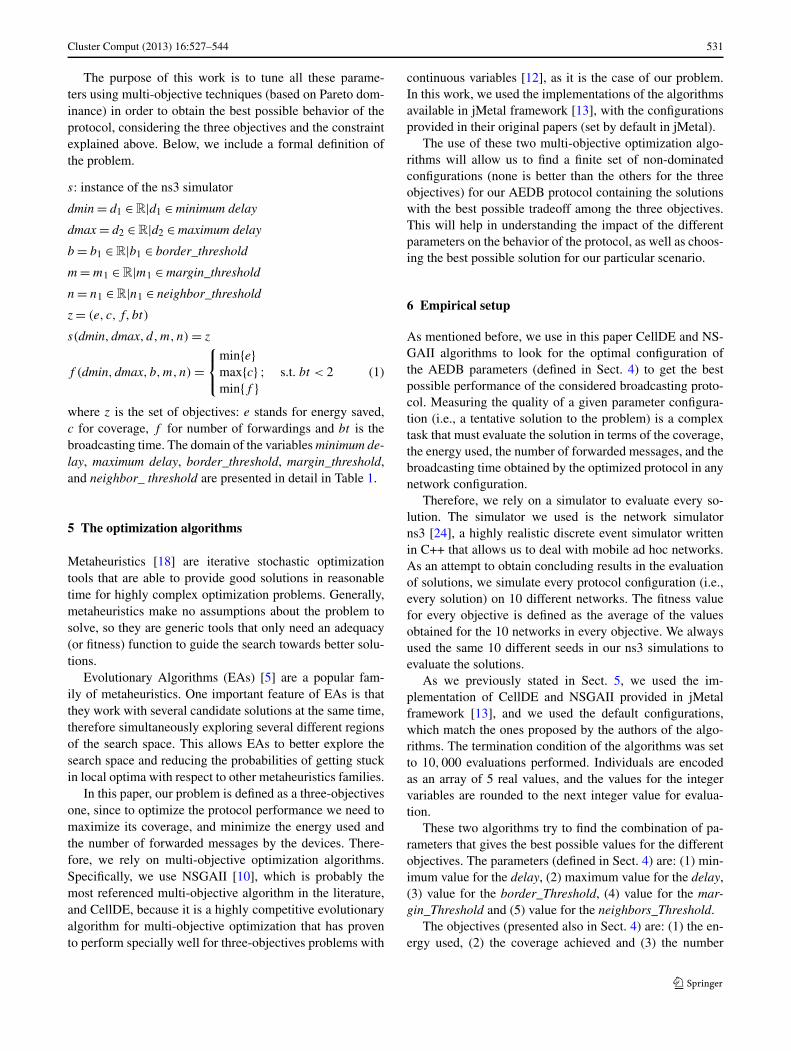
Fig. 1 Comparison of the quality of the fronts computed by the algorithms
reference point W and the solution i as the diagonal cor-ners of the hypercube. The reference point can simply befound by constructing a vector of worst objective functionvalues. Thereafter, a union of all hypercubes is found andits hypervolume (HV) is calculated as:
IHV = volume
( |Q|⋃
i=1
vi
)
. (4)
The higher the value of IHV , the better the approxi-mated Pareto front is.
It can be observed in Eq. (2) that the I+ε indicator makes
use of the optimal Pareto front. Because it is unknown forthe considered problem, we build a reference Pareto frontfrom the solutions reported by the two algorithms in the 30independent runs (they are shown in Fig. 2). In order to avoidpossible bias in the computation of these indicators due tothe different dimensions of the problem objectives, this ref-erence Pareto front is also used to normalize the approxi-mated fronts.
7.1.1 CellDE versus NSGAII
In Fig. 1, we compare the performance of CellDE versusNSGAII for the three problem densities studied according tothe three suggested metrics. In order to get strong statisticalevidence, these results are computed after performing 30 in-dependent runs of every algorithm for each problem density.In the displayed boxplots, the bottom and top of the boxesrepresent the lower and upper quartiles of the data distribu-tion, respectively, while the line between them is the median.The whiskers are the lowest datum still within 1.5 IQR of thelower quartile, and the highest datum still within 1.5 IQR ofthe upper quartile. The circles are data not included betweenthe whiskers. Finally, the notches in the boxes display the
variability of the median between samples. If the notches oftwo boxes are not overlapped, then it means that there arestatistical significant differences in the data with 95 % con-fidence.
The results in Fig. 1 show significant differences betweenthe algorithms in all cases but the I+
ε indicator for the 200and 300 devices network. We can see that NSGAII is provid-ing more accurate results than CellDE, as the boxplots forI+ε and IHV show. Differences are small for I+
ε , and moreimportant in the case of IHV . However, CellDE provides thedecision maker with a much broader choice of tradeoff so-lutions, as the I� plots demonstrate.
Now, we will pay attention on how the algorithms scalewith the problem size. The relative performance of the twoalgorithms is similar for all problem sizes: NSGAII is betterfor I+
ε and IHV , and worse for I�. For I+ε , the boxes are
overlapped for the three network densities, meaning that thesolutions in the first quartile of CellDE are better than thosein the third quartile of NSGAII. Moreover, no significant dif-ferences were found between the algorithms for the densestnetworks. Regarding I�, we can see that the performance ofCellDE with respect to NSGAII improves with the problemdensity, as it can be appreciated by the overlapping degree ofthe whiskers in the boxplots: very high for the 100 devicesproblem, almost null for 200 devices one, and far from beingoverlapped for the densest network. Finally, we observe thatthe difference between the two algorithms is lower for thesmall network than for the other two in the case of IHV too.However, the difference between the algorithms does not in-crease between 200 and 300 devices problems in this case(indeed, it slightly decreases).
7.2 Studying the optimization results
We analyze in this section the quality of the obtained results,and we validate them with the performance of the three orig-
534 Cluster Comput (2013) 16:527–544
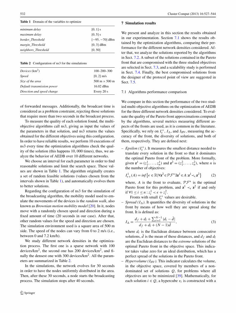
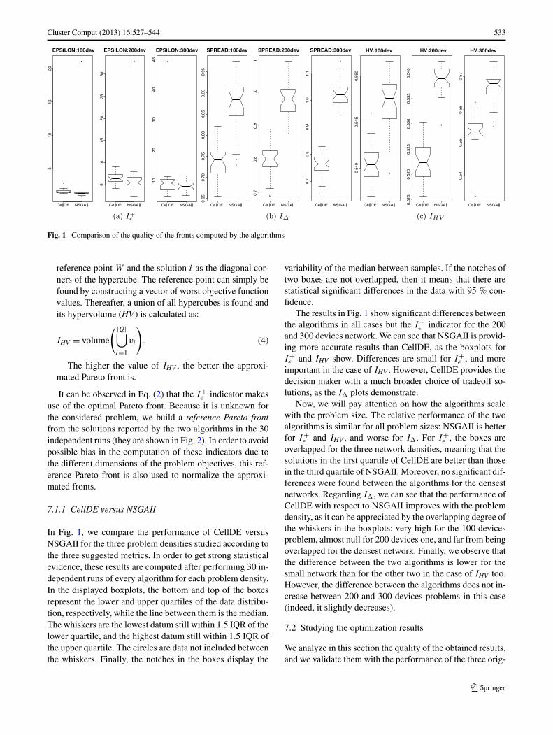
Fig. 2 The reference Pareto fronts obtained after merging all the Pareto front approximations obtained. Black filled circles are the solutions thatwere chosen in this work according to their performance
inal AEDB configurations (three different values of neigh-bors_Threshold parameter were proposed according to thenetwork density). Additionally, we select the five best con-figurations for every density, and evaluate them when scal-ing the network size and density.
As mentioned before, all the different solutions obtainedfor each optimization algorithm were considered to buildone single Pareto front approximation with the best non-dominated solutions found for every network density. Theyare displayed in Fig. 2. The maximum size for these frontswas set to 100 solutions, so when more than 100 non-dominated solutions are available, the best 100 ones, ac-cording to the crowding distance used in NSGAII, are se-lected.
In the Pareto front approximations shown in Fig. 2, itstands out that the fronts have two clear sets of solutionsin the three scenarios. For the lowest energy values in theapproximated range [−20,20] dBm, solutions provide verylow coverage and high number of forwardings, following alinear relationship between these two objectives in whichthe coverage value is similar to the number of forward-ings. These are typically solutions in which devices are onlybroadcasting the message to their closest one, and there-fore the number of forwardings is very close to the numberof devices receiving the message (i.e., the coverage). How-ever, for higher energy values over 20 dBm, the shape of thePareto front changes, and we can see a clearly defined frontof solutions in which coverage values are growing much
Cluster Comput (2013) 16:527–544 535
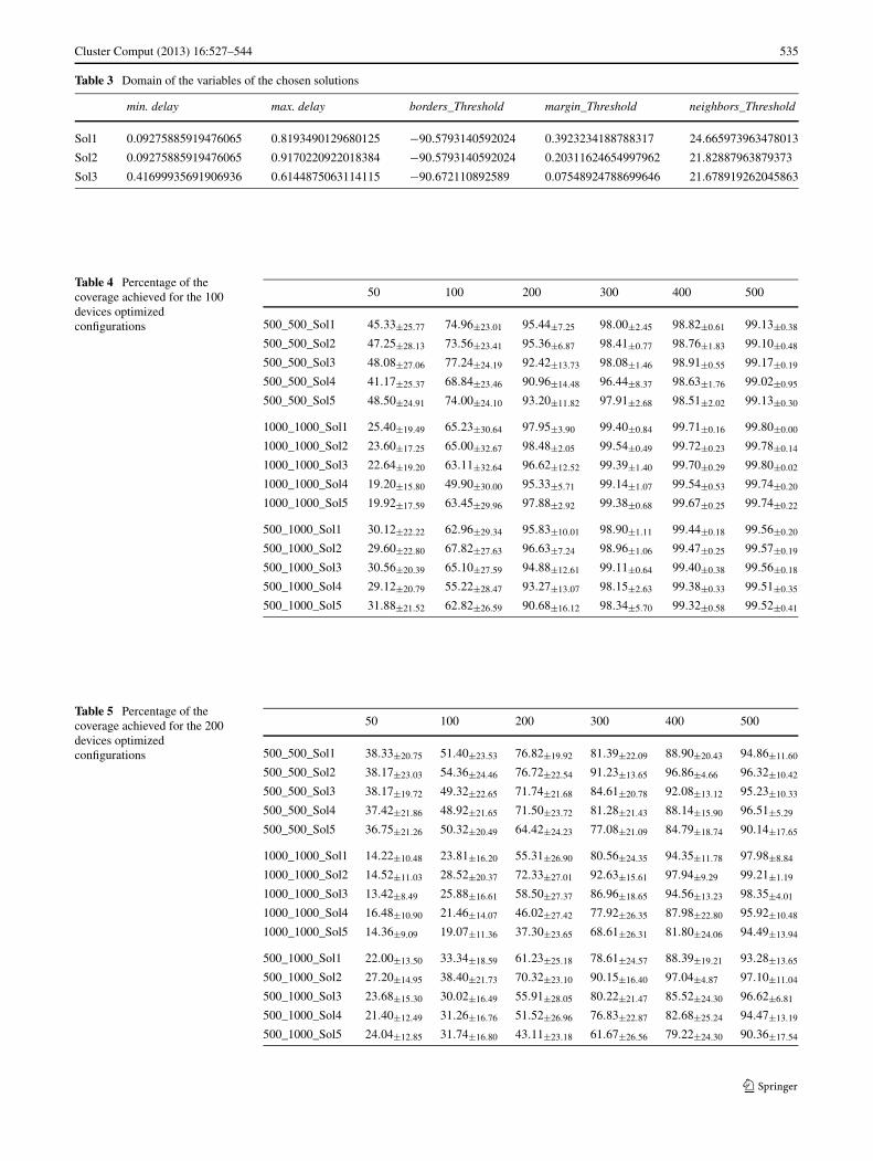
Table 3 Domain of the variables of the chosen solutions
min. delay max. delay borders_Threshold margin_Threshold neighbors_Threshold
Sol1 0.09275885919476065 0.8193490129680125 −90.5793140592024 0.3923234188788317 24.665973963478013
Sol2 0.09275885919476065 0.9170220922018384 −90.5793140592024 0.20311624654997962 21.82887963879373
Sol3 0.41699935691906936 0.6144875063114115 −90.672110892589 0.07548924788699646 21.678919262045863
Table 4 Percentage of thecoverage achieved for the 100devices optimizedconfigurations
50 100 200 300 400 500
500_500_Sol1 45.33±25.77 74.96±23.01 95.44±7.25 98.00±2.45 98.82±0.61 99.13±0.38
500_500_Sol2 47.25±28.13 73.56±23.41 95.36±6.87 98.41±0.77 98.76±1.83 99.10±0.48
500_500_Sol3 48.08±27.06 77.24±24.19 92.42±13.73 98.08±1.46 98.91±0.55 99.17±0.19
500_500_Sol4 41.17±25.37 68.84±23.46 90.96±14.48 96.44±8.37 98.63±1.76 99.02±0.95
500_500_Sol5 48.50±24.91 74.00±24.10 93.20±11.82 97.91±2.68 98.51±2.02 99.13±0.30
1000_1000_Sol1 25.40±19.49 65.23±30.64 97.95±3.90 99.40±0.84 99.71±0.16 99.80±0.00
1000_1000_Sol2 23.60±17.25 65.00±32.67 98.48±2.05 99.54±0.49 99.72±0.23 99.78±0.14
1000_1000_Sol3 22.64±19.20 63.11±32.64 96.62±12.52 99.39±1.40 99.70±0.29 99.80±0.02
1000_1000_Sol4 19.20±15.80 49.90±30.00 95.33±5.71 99.14±1.07 99.54±0.53 99.74±0.20
1000_1000_Sol5 19.92±17.59 63.45±29.96 97.88±2.92 99.38±0.68 99.67±0.25 99.74±0.22
500_1000_Sol1 30.12±22.22 62.96±29.34 95.83±10.01 98.90±1.11 99.44±0.18 99.56±0.20
500_1000_Sol2 29.60±22.80 67.82±27.63 96.63±7.24 98.96±1.06 99.47±0.25 99.57±0.19
500_1000_Sol3 30.56±20.39 65.10±27.59 94.88±12.61 99.11±0.64 99.40±0.38 99.56±0.18
500_1000_Sol4 29.12±20.79 55.22±28.47 93.27±13.07 98.15±2.63 99.38±0.33 99.51±0.35
500_1000_Sol5 31.88±21.52 62.82±26.59 90.68±16.12 98.34±5.70 99.32±0.58 99.52±0.41
Table 5 Percentage of thecoverage achieved for the 200devices optimizedconfigurations
50 100 200 300 400 500
500_500_Sol1 38.33±20.75 51.40±23.53 76.82±19.92 81.39±22.09 88.90±20.43 94.86±11.60
500_500_Sol2 38.17±23.03 54.36±24.46 76.72±22.54 91.23±13.65 96.86±4.66 96.32±10.42
500_500_Sol3 38.17±19.72 49.32±22.65 71.74±21.68 84.61±20.78 92.08±13.12 95.23±10.33
500_500_Sol4 37.42±21.86 48.92±21.65 71.50±23.72 81.28±21.43 88.14±15.90 96.51±5.29
500_500_Sol5 36.75±21.26 50.32±20.49 64.42±24.23 77.08±21.09 84.79±18.74 90.14±17.65
1000_1000_Sol1 14.22±10.48 23.81±16.20 55.31±26.90 80.56±24.35 94.35±11.78 97.98±8.84
1000_1000_Sol2 14.52±11.03 28.52±20.37 72.33±27.01 92.63±15.61 97.94±9.29 99.21±1.19
1000_1000_Sol3 13.42±8.49 25.88±16.61 58.50±27.37 86.96±18.65 94.56±13.23 98.35±4.01
1000_1000_Sol4 16.48±10.90 21.46±14.07 46.02±27.42 77.92±26.35 87.98±22.80 95.92±10.48
1000_1000_Sol5 14.36±9.09 19.07±11.36 37.30±23.65 68.61±26.31 81.80±24.06 94.49±13.94
500_1000_Sol1 22.00±13.50 33.34±18.59 61.23±25.18 78.61±24.57 88.39±19.21 93.28±13.65
500_1000_Sol2 27.20±14.95 38.40±21.73 70.32±23.10 90.15±16.40 97.04±4.87 97.10±11.04
500_1000_Sol3 23.68±15.30 30.02±16.49 55.91±28.05 80.22±21.47 85.52±24.30 96.62±6.81
500_1000_Sol4 21.40±12.49 31.26±16.76 51.52±26.96 76.83±22.87 82.68±25.24 94.47±13.19
500_1000_Sol5 24.04±12.85 31.74±16.80 43.11±23.18 61.67±26.56 79.22±24.30 90.36±17.54
536 Cluster Comput (2013) 16:527–544
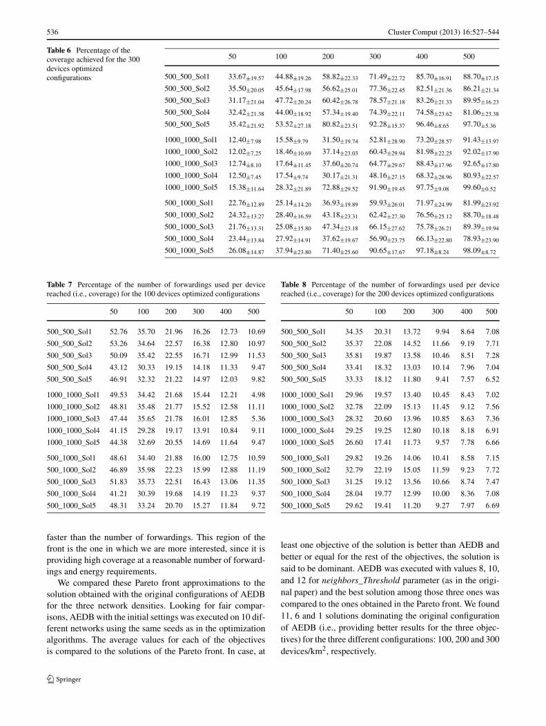
Table 6 Percentage of thecoverage achieved for the 300devices optimizedconfigurations
50 100 200 300 400 500
500_500_Sol1 33.67±19.57 44.88±19.26 58.82±22.33 71.49±22.72 85.70±16.91 88.70±17.15
500_500_Sol2 35.50±20.05 45.64±17.98 56.62±25.01 77.36±22.45 82.51±21.36 86.21±21.34
500_500_Sol3 31.17±21.04 47.72±20.24 60.42±26.78 78.57±21.18 83.26±21.33 89.95±16.23
500_500_Sol4 32.42±21.38 44.00±18.92 57.34±19.40 74.39±22.11 74.58±23.62 81.06±23.38
500_500_Sol5 35.42±21.92 53.52±27.18 80.82±23.51 92.28±15.37 96.46±8.65 97.70±5.36
1000_1000_Sol1 12.40±7.98 15.58±9.79 31.50±19.74 52.81±28.90 73.20±28.57 91.43±13.97
1000_1000_Sol2 12.02±7.25 18.46±10.69 37.14±23.03 60.43±29.94 81.98±22.25 92.02±17.90
1000_1000_Sol3 12.74±8.10 17.64±11.45 37.60±20.74 64.77±29.67 88.43±17.96 92.65±17.80
1000_1000_Sol4 12.50±7.45 17.54±9.74 30.17±21.31 48.16±27.15 68.32±28.96 80.93±22.57
1000_1000_Sol5 15.38±11.64 28.32±21.89 72.88±29.52 91.90±19.45 97.75±9.08 99.60±0.52
500_1000_Sol1 22.76±12.89 25.14±14.20 36.93±19.89 59.93±26.01 71.97±24.99 81.99±23.92
500_1000_Sol2 24.32±13.27 28.40±16.59 43.18±23.31 62.42±27.30 76.56±25.12 88.70±18.48
500_1000_Sol3 21.76±13.31 25.08±15.80 47.34±23.18 66.15±27.62 75.78±26.21 89.39±19.94
500_1000_Sol4 23.44±13.84 27.92±14.91 37.62±19.67 56.90±23.75 66.13±22.80 78.93±23.90
500_1000_Sol5 26.08±14.87 37.94±23.80 71.40±25.60 90.65±17.67 97.18±8.24 98.09±8.72
Table 7 Percentage of the number of forwardings used per devicereached (i.e., coverage) for the 100 devices optimized configurations
50 100 200 300 400 500
500_500_Sol1 52.76 35.70 21.96 16.26 12.73 10.69
500_500_Sol2 53.26 34.64 22.57 16.38 12.80 10.97
500_500_Sol3 50.09 35.42 22.55 16.71 12.99 11.53
500_500_Sol4 43.12 30.33 19.15 14.18 11.33 9.47
500_500_Sol5 46.91 32.32 21.22 14.97 12.03 9.82
1000_1000_Sol1 49.53 34.42 21.68 15.44 12.21 4.98
1000_1000_Sol2 48.81 35.48 21.77 15.52 12.58 11.11
1000_1000_Sol3 47.44 35.65 21.78 16.01 12.85 5.36
1000_1000_Sol4 41.15 29.28 19.17 13.91 10.84 9.11
1000_1000_Sol5 44.38 32.69 20.55 14.69 11.64 9.47
500_1000_Sol1 48.61 34.40 21.88 16.00 12.75 10.59
500_1000_Sol2 46.89 35.98 22.23 15.99 12.88 11.19
500_1000_Sol3 51.83 35.73 22.51 16.43 13.06 11.35
500_1000_Sol4 41.21 30.39 19.68 14.19 11.23 9.37
500_1000_Sol5 48.31 33.24 20.70 15.27 11.84 9.72
faster than the number of forwardings. This region of thefront is the one in which we are more interested, since it isproviding high coverage at a reasonable number of forward-ings and energy requirements.
We compared these Pareto front approximations to thesolution obtained with the original configurations of AEDBfor the three network densities. Looking for fair compar-isons, AEDB with the initial settings was executed on 10 dif-ferent networks using the same seeds as in the optimizationalgorithms. The average values for each of the objectivesis compared to the solutions of the Pareto front. In case, at
Table 8 Percentage of the number of forwardings used per devicereached (i.e., coverage) for the 200 devices optimized configurations
50 100 200 300 400 500
500_500_Sol1 34.35 20.31 13.72 9.94 8.64 7.08
500_500_Sol2 35.37 22.08 14.52 11.66 9.19 7.71
500_500_Sol3 35.81 19.87 13.58 10.46 8.51 7.28
500_500_Sol4 33.41 18.32 13.03 10.14 7.96 7.04
500_500_Sol5 33.33 18.12 11.80 9.41 7.57 6.52
1000_1000_Sol1 29.96 19.57 13.40 10.45 8.43 7.02
1000_1000_Sol2 32.78 22.09 15.13 11.45 9.12 7.56
1000_1000_Sol3 28.32 20.60 13.96 10.85 8.63 7.36
1000_1000_Sol4 29.25 19.25 12.80 10.18 8.18 6.91
1000_1000_Sol5 26.60 17.41 11.73 9.57 7.78 6.66
500_1000_Sol1 29.82 19.26 14.06 10.41 8.58 7.15
500_1000_Sol2 32.79 22.19 15.05 11.59 9.23 7.72
500_1000_Sol3 31.25 19.12 13.56 10.66 8.74 7.47
500_1000_Sol4 28.04 19.77 12.99 10.00 8.36 7.08
500_1000_Sol5 29.62 19.41 11.20 9.27 7.97 6.69
least one objective of the solution is better than AEDB andbetter or equal for the rest of the objectives, the solution issaid to be dominant. AEDB was executed with values 8, 10,and 12 for neighbors_Threshold parameter (as in the origi-nal paper) and the best solution among those three ones wascompared to the ones obtained in the Pareto front. We found11, 6 and 1 solutions dominating the original configurationof AEDB (i.e., providing better results for the three objec-tives) for the three different configurations: 100, 200 and 300devices/km2, respectively.
Cluster Comput (2013) 16:527–544 537
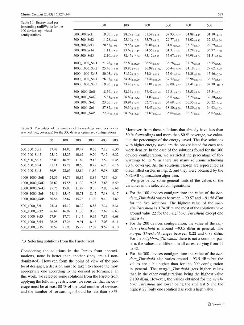
Table 10 Energy used perforwarding (miliWatts) for the100 devices optimizedconfigurations
50 100 200 300 400 500
500_500_Sol1 19.50±15.18 28.29±10.96 31.59±8.06 37.93±5.07 34.89±4.49 31.10±4.33
500_500_Sol2 11.78±8.68 25.10±10.71 33.78±8.03 29.77±3.31 34.02±4.13 32.15±4.24
500_500_Sol3 20.53±7.06 29.55±12.56 30.06±7.98 31.03±4.78 35.72±4.94 29.29±3.72
500_500_Sol4 11.11±12.03 23.68±10.19 34.55±7.71 31.31±8.31 31.28±3.92 35.97±3.80
500_500_Sol5 18.10±10.10 32.45±10.06 35.12±7.13 37.67±4.15 36.98±3.64 31.51±3.80
1000_1000_Sol1 21.78±17.26 32.80±25.20 36.54±8.60 36.28±9.05 37.76±9.78 16.75±3.83
1000_1000_Sol2 25.46±17.36 29.83±26.01 36.99±13.56 36.44±6.39 34.18±5.83 29.62±6.72
1000_1000_Sol3 20.03±18.64 31.39±23.01 34.24±16.81 37.04±9.44 34.28±6.20 15.46±5.06
1000_1000_Sol4 26.95±17.29 34.09±26.29 37.44±15.26 37.52±7.64 36.96±10.48 36.52±8.54
1000_1000_Sol5 19.80±13.94 33.43±20.54 35.01±14.29 38.09±7.67 37.41±10.71 37.30±10.17
500_1000_Sol1 18.39±15.10 32.36±19.25 37.42±10.48 37.31±8.05 35.53±5.54 33.54±6.71
500_1000_Sol2 15.81±10.34 26.82±17.82 34.02±10.37 36.63±5.77 35.24±6.22 32.30±5.52
500_1000_Sol3 23.36±15.83 29.94±17.61 32.77±14.23 34.68±7.35 36.55±7.74 30.22±6.94
500_1000_Sol4 27.82±12.51 29.30±21.23 34.43±14.74 38.80±8.29 35.80±6.29 34.93±6.73
500_1000_Sol5 22.20±15.13 28.97±15.21 35.69±12.72 35.64±7.68 36.27±6.27 35.02±5.83
Table 9 Percentage of the number of forwardings used per devicereached (i.e., coverage) for the 300 devices optimized configurations
50 100 200 300 400 500
500_500_Sol1 27.48 14.80 10.47 8.50 7.18 6.30
500_500_Sol2 25.12 15.25 10.67 9.20 7.42 6.32
500_500_Sol3 32.09 16.93 11.82 9.16 7.59 6.45
500_500_Sol4 31.11 15.27 10.50 8.48 6.70 6.16
500_500_Sol5 36.94 22.65 15.84 11.86 9.38 8.07
1000_1000_Sol1 24.35 14.76 10.87 8.84 7.36 6.34
1000_1000_Sol2 26.62 15.55 11.32 9.25 7.63 6.59
1000_1000_Sol3 25.75 15.93 11.99 9.35 7.90 6.68
1000_1000_Sol4 24.16 15.45 10.71 8.42 7.18 6.17
1000_1000_Sol5 30.56 22.67 15.76 11.90 9.40 7.89
500_1000_Sol1 25.31 15.19 10.32 8.83 7.34 6.31
500_1000_Sol2 26.64 16.97 11.30 9.26 7.69 6.63
500_1000_Sol3 27.94 17.70 11.47 9.65 7.83 6.68
500_1000_Sol4 26.28 17.26 9.91 8.48 7.03 6.11
500_1000_Sol5 30.52 21.98 15.29 12.02 9.52 8.10
7.3 Selecting solutions from the Pareto front
Considering the solutions in the Pareto front approxi-mations, none is better than another (they are all non-dominated). However, from the point of view of the pro-tocol designer, a decision must be taken to choose the mostappropriate one according to the desired performance. Inthis work, we selected some solutions from the Pareto frontapplying the following restrictions: we consider that the cov-erage must be at least 80 % of the total number of devices,and the number of forwardings should be less than 30 %.
Moreover, from those solutions that already have less than30 % forwardings and more than 80 % coverage, we calcu-late the percentage of the energy saved. The five solutionswith higher energy saved are the ones selected for each net-work density. In the case of the solutions found for the 300devices configuration, we restricted the percentage of for-wardings to 15 % as there are many solutions achieving80 % coverage. All the solutions chosen are represented asblack filled circles in Fig. 2, and they were obtained by theNSGAII optimization algorithm.
We give below some general hints of the values of thevariables in the selected configurations:
• For the 100 devices configuration: the value of the bor-ders_Threshold varies between −90.57 and −91.58 dBmfor the five solutions. The highest value of the mar-gin_Threshold is 0.74 dBm and most of the solutions havearound value 22 for the neighbors_Threshold except onethat is 47.
• For the 200 devices configuration: the value of the bor-ders_Threshold is around −93.5 dBm in general. Themargin_Threshold ranges between 0.22 and 0.83 dBm.For the neighbors_Threshold there is not a common pat-tern: the values are different in all cases, varying from 11to 42.
• For the 300 devices configuration: the value of the bor-ders_Threshold also varies around −93.5 dBm but thevalues are a bit higher than for the 200 configurationin general. The margin_Threshold gets higher valuesthan in the other configurations being the highest value2.109 dBm. However, the values obtained for the neigh-bors_Threshold are lower being the smallest 5 and thehighest 28 (only one solution has such a high value).
538 Cluster Comput (2013) 16:527–544
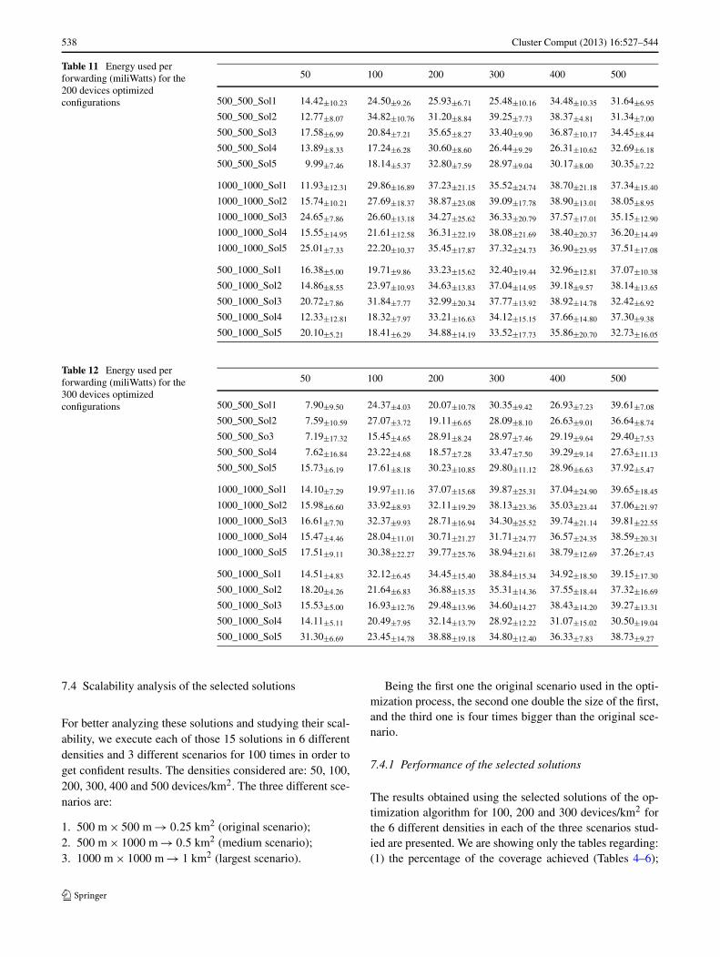
Table 11 Energy used perforwarding (miliWatts) for the200 devices optimizedconfigurations
50 100 200 300 400 500
500_500_Sol1 14.42±10.23 24.50±9.26 25.93±6.71 25.48±10.16 34.48±10.35 31.64±6.95
500_500_Sol2 12.77±8.07 34.82±10.76 31.20±8.84 39.25±7.73 38.37±4.81 31.34±7.00
500_500_Sol3 17.58±6.99 20.84±7.21 35.65±8.27 33.40±9.90 36.87±10.17 34.45±8.44
500_500_Sol4 13.89±8.33 17.24±6.28 30.60±8.60 26.44±9.29 26.31±10.62 32.69±6.18
500_500_Sol5 9.99±7.46 18.14±5.37 32.80±7.59 28.97±9.04 30.17±8.00 30.35±7.22
1000_1000_Sol1 11.93±12.31 29.86±16.89 37.23±21.15 35.52±24.74 38.70±21.18 37.34±15.40
1000_1000_Sol2 15.74±10.21 27.69±18.37 38.87±23.08 39.09±17.78 38.90±13.01 38.05±8.95
1000_1000_Sol3 24.65±7.86 26.60±13.18 34.27±25.62 36.33±20.79 37.57±17.01 35.15±12.90
1000_1000_Sol4 15.55±14.95 21.61±12.58 36.31±22.19 38.08±21.69 38.40±20.37 36.20±14.49
1000_1000_Sol5 25.01±7.33 22.20±10.37 35.45±17.87 37.32±24.73 36.90±23.95 37.51±17.08
500_1000_Sol1 16.38±5.00 19.71±9.86 33.23±15.62 32.40±19.44 32.96±12.81 37.07±10.38
500_1000_Sol2 14.86±8.55 23.97±10.93 34.63±13.83 37.04±14.95 39.18±9.57 38.14±13.65
500_1000_Sol3 20.72±7.86 31.84±7.77 32.99±20.34 37.77±13.92 38.92±14.78 32.42±6.92
500_1000_Sol4 12.33±12.81 18.32±7.97 33.21±16.63 34.12±15.15 37.66±14.80 37.30±9.38
500_1000_Sol5 20.10±5.21 18.41±6.29 34.88±14.19 33.52±17.73 35.86±20.70 32.73±16.05
Table 12 Energy used perforwarding (miliWatts) for the300 devices optimizedconfigurations
50 100 200 300 400 500
500_500_Sol1 7.90±9.50 24.37±4.03 20.07±10.78 30.35±9.42 26.93±7.23 39.61±7.08
500_500_Sol2 7.59±10.59 27.07±3.72 19.11±6.65 28.09±8.10 26.63±9.01 36.64±8.74
500_500_So3 7.19±17.32 15.45±4.65 28.91±8.24 28.97±7.46 29.19±9.64 29.40±7.53
500_500_Sol4 7.62±16.84 23.22±4.68 18.57±7.28 33.47±7.50 39.29±9.14 27.63±11.13
500_500_Sol5 15.73±6.19 17.61±8.18 30.23±10.85 29.80±11.12 28.96±6.63 37.92±5.47
1000_1000_Sol1 14.10±7.29 19.97±11.16 37.07±15.68 39.87±25.31 37.04±24.90 39.65±18.45
1000_1000_Sol2 15.98±6.60 33.92±8.93 32.11±19.29 38.13±23.36 35.03±23.44 37.06±21.97
1000_1000_Sol3 16.61±7.70 32.37±9.93 28.71±16.94 34.30±25.52 39.74±21.14 39.81±22.55
1000_1000_Sol4 15.47±4.46 28.04±11.01 30.71±21.27 31.71±24.77 36.57±24.35 38.59±20.31
1000_1000_Sol5 17.51±9.11 30.38±22.27 39.77±25.76 38.94±21.61 38.79±12.69 37.26±7.43
500_1000_Sol1 14.51±4.83 32.12±6.45 34.45±15.40 38.84±15.34 34.92±18.50 39.15±17.30
500_1000_Sol2 18.20±4.26 21.64±6.83 36.88±15.35 35.31±14.36 37.55±18.44 37.32±16.69
500_1000_Sol3 15.53±5.00 16.93±12.76 29.48±13.96 34.60±14.27 38.43±14.20 39.27±13.31
500_1000_Sol4 14.11±5.11 20.49±7.95 32.14±13.79 28.92±12.22 31.07±15.02 30.50±19.04
500_1000_Sol5 31.30±6.69 23.45±14.78 38.88±19.18 34.80±12.40 36.33±7.83 38.73±9.27
7.4 Scalability analysis of the selected solutions
For better analyzing these solutions and studying their scal-ability, we execute each of those 15 solutions in 6 differentdensities and 3 different scenarios for 100 times in order toget confident results. The densities considered are: 50, 100,200, 300, 400 and 500 devices/km2. The three different sce-narios are:
1. 500 m × 500 m → 0.25 km2 (original scenario);2. 500 m × 1000 m → 0.5 km2 (medium scenario);3. 1000 m × 1000 m → 1 km2 (largest scenario).
Being the first one the original scenario used in the opti-mization process, the second one double the size of the first,and the third one is four times bigger than the original sce-nario.
7.4.1 Performance of the selected solutions
The results obtained using the selected solutions of the op-timization algorithm for 100, 200 and 300 devices/km2 forthe 6 different densities in each of the three scenarios stud-ied are presented. We are showing only the tables regarding:(1) the percentage of the coverage achieved (Tables 4–6);
Cluster Comput (2013) 16:527–544 539
Table 13 Percentage of the energy saved per forwarding (miliWatts)for the 100 devices optimized configurations
50 100 200 300 400 500
500_500_Sol1 51.24 29.27 21.03 5.18 12.78 22.24
500_500_Sol2 70.56 37.26 15.54 25.59 14.95 19.61
500_500_Sol3 48.68 26.11 24.85 22.44 10.69 26.78
500_500_Sol4 72.22 40.80 13.62 21.72 21.81 10.06
500_500_Sol5 54.76 18.89 12.19 5.83 7.54 21.23
1000_1000_Sol1 45.55 18.00 8.64 9.29 5.61 58.12
1000_1000_Sol2 36.36 25.42 7.51 8.90 14.56 25.95
1000_1000_Sol3 49.93 21.53 14.40 7.39 14.30 61.35
1000_1000_Sol4 32.62 14.78 6.40 6.21 7.60 8.71
1000_1000_Sol5 50.51 16.43 12.48 4.78 6.46 6.74
500_1000_Sol1 54.01 19.09 6.44 6.72 11.17 16.15
500_1000_Sol2 60.46 32.94 14.95 8.43 11.90 19.24
500_1000_Sol3 41.59 25.15 18.06 13.30 8.64 24.45
500_1000_Sol4 30.45 26.75 13.91 3.00 10.49 12.69
500_1000_Sol5 44.50 27.59 10.78 10.90 9.32 12.45
Table 14 Percentage of the energy saved per forwarding (miliWatts)for the 200 devices optimized configurations
50 100 200 300 400 500
500_500_Sol1 63.95 38.76 35.19 36.30 13.81 20.89
500_500_Sol2 68.07 12.95 22.01 1.87 4.08 21.64
500_500_Sol3 56.06 47.91 10.88 16.49 7.84 13.87
500_500_Sol4 65.27 56.90 23.49 33.91 34.23 18.28
500_500_Sol5 75.03 54.64 17.99 27.58 24.58 24.13
1000_1000_Sol1 70.17 25.35 6.92 11.20 3.25 6.65
1000_1000_Sol2 60.65 30.77 2.82 2.28 2.74 4.88
1000_1000_Sol3 38.38 33.50 14.33 9.18 6.07 12.14
1000_1000_Sol4 61.12 45.97 9.23 4.81 4.00 9.49
1000_1000_Sol5 37.49 44.49 11.37 6.71 7.76 6.22
500_1000_Sol1 59.05 50.73 16.93 18.99 17.59 7.33
500_1000_Sol2 62.85 40.08 13.42 7.39 2.04 4.66
500_1000_Sol3 48.19 20.39 17.53 5.57 2.70 18.96
500_1000_Sol4 69.18 54.21 16.98 14.70 5.85 6.75
500_1000_Sol5 49.75 53.98 12.79 16.20 10.35 18.18
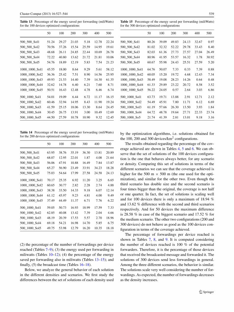
(2) the percentage of the number of forwardings per devicereached (Tables 7–9); (3) the energy used per forwarding inmiliwatts (Tables 10–12); (4) the percentage of the energysaved per forwarding also in miliwatts (Tables 13–15); andfinally, (5) the broadcast time (Tables 16–18).
Below, we analyze the general behavior of each solutionin the different densities and scenarios. We first study thedifferences between the set of solutions of each density used
Table 15 Percentage of the energy saved per forwarding (miliWatts)for the 300 devices optimized configurations
50 100 200 300 400 500
500_500_Sol1 80.26 39.09 49.83 24.13 32.67 0.97
500_500_Sol2 81.02 32.32 52.22 29.78 33.43 8.40
500_500_Sol3 82.03 61.36 27.73 27.57 27.04 26.49
500_500_Sol4 80.96 41.95 53.57 16.32 1.78 30.92
500_500_Sol5 60.67 55.98 24.43 25.51 27.59 5.20
1000_1000_Sol1 64.76 50.07 7.33 0.33 7.39 0.88
1000_1000_Sol2 60.05 15.20 19.72 4.68 12.43 7.34
1000_1000_Sol3 58.49 19.08 28.23 14.26 0.64 0.48
1000_1000_Sol4 61.33 29.89 23.22 20.72 8.58 3.52
1000_1000_Sol5 56.22 24.05 0.57 2.64 3.03 6.86
500_1000_Sol1 63.73 19.71 13.88 2.91 12.71 2.12
500_1000_Sol2 54.49 45.91 7.80 11.71 6.12 6.69
500_1000_Sol3 61.19 57.66 26.30 13.50 3.93 1.84
500_1000_Sol4 64.72 48.78 19.64 27.71 22.33 23.74
500_1000_So5 21.74 41.39 2.81 13.01 9.18 3.16
by the optimization algorithms, i.e. solutions obtained forthe 100, 200 and 300 devices/km2 configurations.
The results obtained regarding the percentage of the cov-erage achieved are shown in Tables 4, 5 and 6. We can ob-serve that the set of solutions of the 100 devices configura-tion is the one that behaves always better, for any scenarioor density. Comparing this set of solutions in terms of thedifferent scenarios we can see that the coverage achieved ishigher for the 500 m × 500 m (the one used for the opti-mization), and similar for the other two. Even though thethird scenario has double size and the second scenario isfour times bigger than the original, the coverage is not halfor one quarter. In fact, the set of solutions is scaling welland for 100 devices there is only a maximum of 18.94 %and 13.62 % difference with the second and third scenariosrespectively. And for 50 devices the maximum differenceis 28.58 % in case of the biggest scenario and 17.52 % forthe medium scenario. The other two configurations (200 and300 devices) do not behave as good as the 100 devices con-figuration in terms of the coverage achieved.
The percentage of forwardings per device reached isshown in Tables 7, 8, and 9. It is computed consideringthe number of devices reached is 100 % of the potentialforwarders. Therefore, it is the percentage of those devicesthat received the broadcasted message and forwarded it. Thesolutions of 300 devices send less forwardings in general.Among the three different scenarios, the behavior is similar.The solutions scale very well considering the number of for-wardings. As expected, the number of forwardings decreasesas the density increases.
540 Cluster Comput (2013) 16:527–544
Fig. 3 Energy saved per forwarding for each of the scenarios studied
In terms of the energy savings, we show in Tables 13, 14and 15 the percentage of energy saved per forwarding. Theenergy saved is calculated as:
EgSaved = #forwardings × DefTx − EgUsed
#forwardings. (5)
That is, the difference between the energy used in case allthe nodes sending the message are using the default trans-mission power and the actual energy used by the protocol(in miliWatts), divided by the number of forwardings.
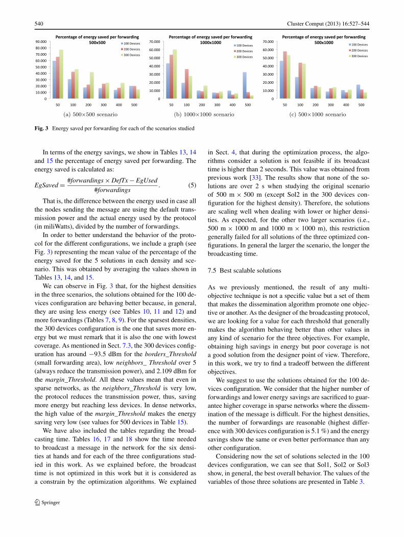
In order to better understand the behavior of the proto-col for the different configurations, we include a graph (seeFig. 3) representing the mean value of the percentage of theenergy saved for the 5 solutions in each density and sce-nario. This was obtained by averaging the values shown inTables 13, 14, and 15.
We can observe in Fig. 3 that, for the highest densitiesin the three scenarios, the solutions obtained for the 100 de-vices configuration are behaving better because, in general,they are using less energy (see Tables 10, 11 and 12) andmore forwardings (Tables 7, 8, 9). For the sparsest densities,the 300 devices configuration is the one that saves more en-ergy but we must remark that it is also the one with lowestcoverage. As mentioned in Sect. 7.3, the 300 devices config-uration has around −93.5 dBm for the borders_Threshold(small forwarding area), low neighbors_ Threshold over 5(always reduce the transmission power), and 2.109 dBm forthe margin_Threshold. All these values mean that even insparse networks, as the neighbors_Threshold is very low,the protocol reduces the transmission power, thus, savingmore energy but reaching less devices. In dense networks,the high value of the margin_Threshold makes the energysaving very low (see values for 500 devices in Table 15).
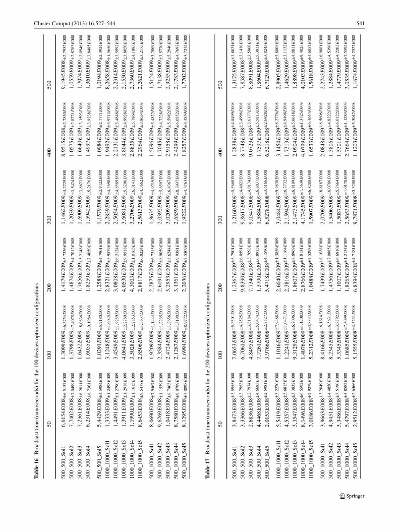
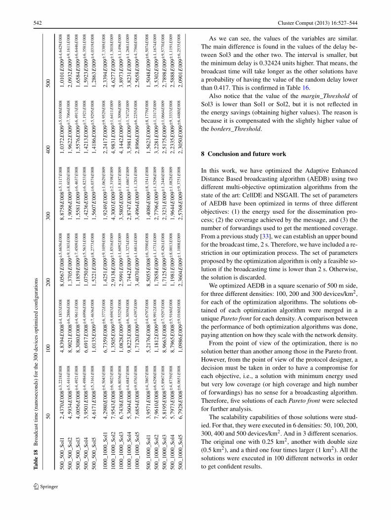
We have also included the tables regarding the broad-casting time. Tables 16, 17 and 18 show the time neededto broadcast a message in the network for the six densi-ties at hands and for each of the three configurations stud-ied in this work. As we explained before, the broadcasttime is not optimized in this work but it is considered asa constrain by the optimization algorithms. We explained
in Sect. 4, that during the optimization process, the algo-rithms consider a solution is not feasible if its broadcasttime is higher than 2 seconds. This value was obtained fromprevious work [33]. The results show that none of the so-lutions are over 2 s when studying the original scenarioof 500 m × 500 m (except Sol2 in the 300 devices con-figuration for the highest density). Therefore, the solutionsare scaling well when dealing with lower or higher densi-ties. As expected, for the other two larger scenarios (i.e.,500 m × 1000 m and 1000 m × 1000 m), this restrictiongenerally failed for all solutions of the three optimized con-figurations. In general the larger the scenario, the longer thebroadcasting time.
7.5 Best scalable solutions
As we previously mentioned, the result of any multi-objective technique is not a specific value but a set of themthat makes the dissemination algorithm promote one objec-tive or another. As the designer of the broadcasting protocol,we are looking for a value for each threshold that generallymakes the algorithm behaving better than other values inany kind of scenario for the three objectives. For example,obtaining high savings in energy but poor coverage is nota good solution from the designer point of view. Therefore,in this work, we try to find a tradeoff between the differentobjectives.
We suggest to use the solutions obtained for the 100 de-vices configuration. We consider that the higher number offorwardings and lower energy savings are sacrificed to guar-antee higher coverage in sparse networks where the dissem-ination of the message is difficult. For the highest densities,the number of forwardings are reasonable (highest differ-ence with 300 devices configuration is 5.1 %) and the energysavings show the same or even better performance than anyother configuration.
Considering now the set of solutions selected in the 100devices configuration, we can see that Sol1, Sol2 or Sol3show, in general, the best overall behavior. The values of thevariables of those three solutions are presented in Table 3.
Cluster Comput (2013) 16:527–544 541
Tabl
e16
Bro
adca
sttim
e(n
anos
econ
ds)
for
the
100
devi
ces
optim
ized
confi
gura
tions
5010
020
030
040
050
0
500_
500_
Sol1
6,61
54E
008 ±
6,51
57E
008
1,30
99E
009 ±
6,57
54E
008
1,41
79E
009 ±
5,73
36E
008
1,14
62E
009 ±
4,27
29E
008
8,95
15E
008 ±
2,78
30E
008
9,19
45E
008 ±
2,79
52E
008
500_
500_
Sol2
7,74
02E
008 ±
7,04
99E
008
1,37
98E
009 ±
7,40
75E
008
1,48
74E
009 ±
4,70
12E
008
1,20
39E
009 ±
3,54
24E
008
1,05
75E
009 ±
2,87
21E
008
1,05
59E
009 ±
2,82
83E
008
500_
500_
Sol3
7,23
61E
008 ±
6,20
11E
008
1,64
32E
009 ±
8,08
36E
008
1,76
56E
009 ±
5,21
48E
008
1,69
09E
009 ±
3,66
23E
008
1,66
40E
009 ±
3,15
93E
008
1,70
74E
009 ±
3,09
46E
008
500_
500_
Sol4
6,23
14E
008 ±
6,73
61E
008
1,60
55E
009 ±
9,19
84E
008
1,82
59E
009 ±
7,40
59E
008
1,59
42E
009 ±
5,21
76E
008
1,49
97E
009 ±
3,92
38E
008
1,36
10E
009 ±
3,84
85E
008
500_
500_
Sol5
5,44
29E
008 ±
4,59
84E
008
1,02
91E
009 ±
5,21
80E
008
1,25
88E
009 ±
4,79
01E
008
1,15
79E
009 ±
2,94
22E
008
1,09
84E
009 ±
2,77
71E
008
1,01
94E
009 ±
2,39
24E
008
1000
_100
0_So
l11,
3333
E00
9 ±1,
2498
E00
93,
1248
E00
9 ±1,
6045
E00
92,
8321
E00
9 ±5,
9579
E00
82,
2839
E00
9 ±4,
5698
E00
81,
9492
E00
9 ±3,
9714
E00
88,
2658
E00
8 ±1,
5656
E00
8
1000
_100
0_So
l21,
4491
E00
9 ±1,
2790
E00
93,
4549
E00
9 ±1,
9259
E00
93,
0808
E00
9 ±6,
2124
E00
82,
5054
E00
9 ±4,
8589
E00
82,
2131
E00
9 ±3,
4848
E00
82,
2314
E00
9 ±3,
5992
E00
8
1000
_100
0_So
l31,
3911
E00
9 ±1,
2918
E00
94,
0641
E00
9 ±2,
2789
E00
94,
0530
E00
9 ±9,
9518
E00
83,
6081
E00
9 ±5,
3206
E00
83,
8044
E00
9 ±4,
9928
E00
82,
1550
E00
9 ±3,
8050
E00
8
1000
_100
0_So
l41,
1990
E00
9 ±1,
1615
E00
93,
5028
E00
9 ±2,
2853
E00
94,
3003
E00
9 ±1,
0163
E00
93,
2706
E00
9 ±6,
3141
E00
82,
8835
E00
9 ±5,
7864
E00
82,
7360
E00
9 ±4,
1883
E00
8
1000
_100
0_So
l58,
6453
E00
8 ±9,
5478
E00
82,
8506
E00
9 ±1,
5637
E00
92,
8817
E00
9 ±6,
8224
E00
82,
5613
E00
9 ±4,
3662
E00
82,
2964
E00
9 ±3,
8654
E00
82,
2621
E00
9 ±3,
2175
E00
8
500_
1000
_Sol
18,
0690
E00
8 ±7,
9467
E00
81,
9209
E00
9 ±1,
1444
E00
92,
2875
E00
9 ±6,
7315
E00
81,
8635
E00
9 ±4,
9219
E00
81,
5096
E00
9 ±3,
4822
E00
81,
5124
E00
9 ±3,
2009
E00
8
500_
1000
_Sol
29,
6769
E00
8 ±1,
1539
E00
92,
3584
E00
9 ±1,
2235
E00
92,
6191
E00
9 ±8,
9059
E00
82,
0392
E00
9 ±5,
6597
E00
81,
7045
E00
9 ±4,
7228
E00
81,
7138
E00
9 ±3,
5770
E00
8
500_
1000
_Sol
31,
0418
E00
9 ±8,
7463
E00
82,
4724
E00
9 ±1,
2656
E00
93,
2953
E00
9 ±8,
6244
E00
83,
0209
E00
9 ±6,
4367
E00
82,
9158
E00
9 ±5,
5982
E00
82,
9255
E00
9 ±5,
2940
E00
8
500_
1000
_Sol
48,
7580
E00
8 ±9,
0799
E00
82,
1287
E00
9 ±1,
3190
E00
93,
1361
E00
9 ±9,
9381
E00
82,
6859
E00
9 ±8,
3037
E00
82,
4299
E00
9 ±6,
0552
E00
82,
1783
E00
9 ±4,
7697
E00
8
500_
1000
_Sol
58,
1295
E00
8 ±7,
0898
E00
81,
6994
E00
9 ±8,
9772
E00
82,
2036
E00
9 ±7,
5509
E00
81,
9222
E00
9 ±4,
3763
E00
81,
8257
E00
9 ±3,
4859
E00
81,
7702
E00
9 ±3,
7212
E00
8
Tabl
e17
Bro
adca
sttim
e(n
anos
econ
ds)
for
the
200
devi
ces
optim
ized
confi
gura
tions
5010
020
030
040
050
0
500_
500_
Sol1
3,84
73E
008±
3,59
55E
008
7,06
53E
008±
5,35
01E
008
1,23
67E
009±
5,79
01E
008
1,21
60E
009±
5,56
60E
008
1,28
38E
009±
4,84
99E
008
1,31
75E
009±
3,80
31E
008
500_
500_
Sol2
3,33
66E
008±
3,79
53E
008
6,70
61E
008±
4,75
25E
008
9,83
90E
008±
6,05
91E
008
9,86
17E
008±
4,40
23E
008
8,77
48E
008±
3,49
96E
008
7,85
87E
008±
3,14
16E
008
500_
500_
Sol3
2,68
36E
008±
2,79
74E
008
4,84
95E
008±
3,81
84E
008
7,73
40E
008±
3,70
93E
008
9,03
47E
008±
4,01
74E
008
9,07
23E
008±
3,61
77E
008
8,80
91E
008±
3,58
60E
008
500_
500_
Sol4
4,44
68E
008±
4,66
83E
008
7,72
61E
008±
5,04
74E
008
1,37
90E
009±
6,89
13E
008
1,58
84E
009±
6,80
37E
008
1,75
97E
009±
5,58
13E
008
1,86
04E
009±
5,38
11E
008
500_
500_
Sol5
2,01
53E
008±
2,59
81E
008
3,97
66E
008±
2,75
27E
008
5,47
18E
008±
4,15
90E
008
6,52
78E
008±
3,51
66E
008
6,52
18E
008±
2,69
28E
008
6,71
29E
008±
3,02
43E
008
1000
_100
0_So
l15,
5419
E00
8±5,
2270
E00
81,
1016
E00
9±7,
9488
E00
82,
6040
E00
9±1,
3856
E00
93,
0484
E00
9±9,
9830
E00
83,
1454
E00
9±8,
2776
E00
82,
8905
E00
9±5,
8808
E00
8
1000
_100
0_So
l24,
5357
E00
8±5,
6815
E00
81,
2241
E00
9±1,
0471
E00
92,
3816
E00
9±1,
1164
E00
92,
1594
E00
9±6,
7732
E00
81,
7313
E00
9±4,
9498
E00
81,
4629
E00
9±3,
1132
E00
8
1000
_100
0_So
l33,
3547
E00
8±3,
3832
E00
89,
3129
E00
8±6,
7096
E00
81,
8607
E00
9±8,
8969
E00
82,
1473
E00
9±6,
8109
E00
82,
0904
E00
9±5,
6618
E00
81,
8898
E00
9±4,
0811
E00
8
1000
_100
0_So
l48,
1496
E00
8±6,
5592
E00
81,
4076
E00
9±1,
1208
E00
92,
8766
E00
9±1,
8131
E00
94,
1745
E00
9±1,
5639
E00
94,
0799
E00
9±1,
3725
E00
94,
0103
E00
9±9,
4025
E00
8
1000
_100
0_So
l53,
0186
E00
8±2,
9279
E00
85,
2312
E00
8±3,
8334
E00
81,
0488
E00
9±7,
5293
E00
81,
5907
E00
9±6,
8288
E00
81,
6533
E00
9±6,
4644
E00
81,
5618
E00
9±4,
6857
E00
8
500_
1000
_Sol
13,
9663
E00
8±3,
2049
E00
88,
4166
E00
8±6,
1614
E00
81,
7439
E00
9±8,
1038
E00
82,
0709
E00
9±8,
6187
E00
82,
0848
E00
9±6,
5696
E00
82,
2743
E00
9±6,
9881
E00
8
500_
1000
_Sol
24,
9451
E00
8±4,
4850
E00
88,
2345
E00
8±6,
5631
E00
81,
4756
E00
9±7,
0885
E00
81,
5406
E00
9±6,
0786
E00
81,
3806
E00
9±4,
8222
E00
81,
2884
E00
9±4,
5390
E00
8
500_
1000
_Sol
33,
3486
E00
8±3,
5190
E00
85,
3345
E00
8±3,
8792
E00
81,
1007
E00
9±6,
6910
E00
81,
5087
E00
9±5,
7664
E00
81,
5301
E00
9±6,
0122
E00
81,
4779
E00
9±4,
2202
E00
8
500_
1000
_Sol
45,
4797
E00
8±4,
8582
E00
81,
0685
E00
9±7,
3099
E00
81,
8265
E00
9±1,
2154
E00
92,
5653
E00
9±1,
0178
E00
92,
7664
E00
9±1,
1283
E00
93,
0535
E00
9±7,
5592
E00
8
500_
1000
_Sol
52,
9512
E00
8±2,
6466
E00
85,
1555
E00
8±4,
3231
E00
86,
8394
E00
8±4,
7181
E00
89,
7871
E00
8±5,
3208
E00
81,
1203
E00
9±5,
5042
E00
81,
1674
E00
9±4,
2527
E00
8
542 Cluster Comput (2013) 16:527–544
Tabl
e18
Bro
adca
sttim
e(n
anos
econ
ds)
for
the
300
devi
ces
optim
ized
confi
gura
tions
5010
020
030
040
050
0
500_
500_
Sol1
2,43
70E
008±
3,22
18E
008
4,83
94E
008±
4,18
33E
008
8,05
67E
008±
5,66
56E
008
8,87
58E
008±
5,11
17E
008
1,03
72E
009±
5,01
00E
008
1,01
01E
009±
4,64
29E
008
500_
500_
Sol2
4,59
34E
008±
5,44
14E
008
8,90
21E
008±
6,28
86E
008
1,37
05E
009±
9,13
03E
008
1,90
96E
009±
8,60
20E
008
1,96
22E
009±
7,70
64E
008
2,09
32E
009±
9,16
11E
008
500_
500_
Sol3
4,00
56E
008±
4,49
21E
008
8,30
80E
008±
4,96
11E
008
1,18
59E
009±
7,45
09E
008
1,55
81E
009±
6,46
37E
008
1,55
76E
009±
6,49
13E
008
1,65
84E
009±
6,64
46E
008
500_
500_
Sol4
3,95
01E
008±
4,49
84E
008
6,69
17E
008±
4,69
96E
008
1,07
50E
009±
5,56
31E
008
1,42
36E
009±
6,82
33E
008
1,42
13E
009±
7,19
21E
008
1,59
23E
009±
6,35
81E
008
500_
500_
Sol5
4,61
71E
008±
5,31
61E
008
1,01
35E
009±
7,46
36E
008
1,52
21E
009±
8,27
73E
008
1,56
07E
009±
6,03
74E
008
1,41
86E
009±
5,92
95E
008
1,28
63E
009±
4,03
19E
008
1000
_100
0_So
l14,
2980
E00
8±4,
5043
E00
86,
7359
E00
8±6,
3772
E00
81,
4251
E00
9±9,
1059
E00
81,
9249
E00
9±1,
0629
E00
92,
2417
E00
9±9,
9529
E00
82,
3394
E00
9±7,
3389
E00
8
1000
_100
0_So
l27,
9543
E00
8±6,
9023
E00
81,
3505
E00
9±9,
6943
E00
82,
9138
E00
9±1,
8516
E00
94,
3003
E00
9±2,
3198
E00
94,
9831
E00
9±1,
6411
E00
94,
6277
E00
9±1,
3018
E00
9
1000
_100
0_So
l36,
7438
E00
8±6,
8036
E00
81,
0828
E00
9±9,
5325
E00
82,
5991
E00
9±1,
6092
E00
93,
5805
E00
9±1,
8187
E00
94,
1442
E00
9±1,
3096
E00
93,
8973
E00
9±1,
1496
E00
9
1000
_100
0_So
l45,
3604
E00
8±4,
6847
E00
89,
8223
E00
8±6,
3039
E00
81,
7442
E00
9±1,
3274
E00
92,
8747
E00
9±1,
6867
E00
93,
5981
E00
9±1,
7472
E00
93,
8231
E00
9±1,
2681
E00
9
1000
_100
0_So
l57,
6854
E00
8±9,
0763
E00
81,
7120
E00
9±1,
4397
E00
93,
4070
E00
9±1,
6814
E00
93,
4964
E00
9±1,
1201
E00
92,
8966
E00
9±6,
2255
E00
82,
5658
E00
9±4,
7560
E00
8
500_
1000
_Sol
13,
9571
E00
8±4,
3867
E00
85,
2176
E00
8±4,
6797
E00
88,
5055
E00
8±6,
3590
E00
81,
4086
E00
9±8,
1541
E00
81,
5623
E00
9±8,
1779
E00
81,
5048
E00
9±6,
5074
E00
8
500_
1000
_Sol
27,
9610
E00
8±6,
6290
E00
81,
1812
E00
9±8,
9912
E00
81,
7858
E00
9±1,
1731
E00
92,
7796
E00
9±1,
5296
E00
93,
2281
E00
9±1,
3317
E00
93,
5302
E00
9±1,
1674
E00
9
500_
1000
_Sol
35,
8195
E00
8±5,
8967
E00
88,
9663
E00
8±7,
9297
E00
81,
7125
E00
9±9,
4261
E00
82,
3231
E00
9±1,
2440
E00
92,
5175
E00
9±1,
0664
E00
92,
7898
E00
9±9,
5770
E00
8
500_
1000
_Sol
45,
7973
E00
8±4,
8739
E00
88,
7965
E00
8±5,
9160
E00
81,
1981
E00
9±8,
0013
E00
81,
9644
E00
9±1,
0828
E00
92,
2335
E00
9±9,
3333
E00
82,
5888
E00
9±1,
1191
E00
9
500_
1000
_Sol
56,
7928
E00
8±6,
0651
E00
81,
0986
E00
9±9,
0160
E00
82,
3604
E00
9±1,
1008
E00
92,
5768
E00
9±9,
3751
E00
82,
3050
E00
9±6,
4480
E00
82,
0901
E00
9±6,
2535
E00
8
As we can see, the values of the variables are similar.The main difference is found in the values of the delay be-tween Sol3 and the other two. The interval is smaller, butthe minimum delay is 0.32424 units higher. That means, thebroadcast time will take longer as the other solutions havea probability of having the value of the random delay lowerthan 0.417. This is confirmed in Table 16.
Also notice that the value of the margin_Threshold ofSol3 is lower than Sol1 or Sol2, but it is not reflected inthe energy savings (obtaining higher values). The reason isbecause it is compensated with the slightly higher value ofthe borders_Threshold.
8 Conclusion and future work
In this work, we have optimized the Adaptive EnhancedDistance Based broadcasting algorithm (AEDB) using twodifferent multi-objective optimization algorithms from thestate of the art: CellDE and NSGAII. The set of parametersof AEDB have been optimized in terms of three differentobjectives: (1) the energy used for the dissemination pro-cess; (2) the coverage achieved by the message, and (3) thenumber of forwardings used to get the mentioned coverage.From a previous study [33], we can establish an upper boundfor the broadcast time, 2 s. Therefore, we have included a re-striction in our optimization process. The set of parametersproposed by the optimization algorithm is only a feasible so-lution if the broadcasting time is lower than 2 s. Otherwise,the solution is discarded.
We optimized AEDB in a square scenario of 500 m side,for three different densities: 100, 200 and 300 devices/km2,for each of the optimization algorithms. The solutions ob-tained of each optimization algorithm were merged in aunique Pareto front for each density. A comparison betweenthe performance of both optimization algorithms was done,paying attention on how they scale with the network density.
From the point of view of the optimization, there is nosolution better than another among those in the Pareto front.However, from the point of view of the protocol designer, adecision must be taken in order to have a compromise foreach objective, i.e., a solution with minimum energy usedbut very low coverage (or high coverage and high numberof forwardings) has no sense for a broadcasting algorithm.Therefore, five solutions of each Pareto front were selectedfor further analysis.
The scalability capabilities of those solutions were stud-ied. For that, they were executed in 6 densities: 50, 100, 200,300, 400 and 500 devices/km2. And in 3 different scenarios.The original one with 0.25 km2, another with double size(0.5 km2), and a third one four times larger (1 km2). All thesolutions were executed in 100 different networks in orderto get confident results.
Cluster Comput (2013) 16:527–544 543
A deep study was performed in order to analyze the scal-ability of the different solutions in terms of: (1) the percent-age of the coverage achieved; (2) the percentage of forward-ings per device reached in the broadcasting process; and (3)the percentage of energy used and saved both in miliWatts.Finally, the broadcast time was also included in the analysis.
From all the results, we suggested that the set of solu-tions that generally behave and scale better were the onesfound in the Pareto front approximation obtained for 100devices/km2 density. Among the five solutions selected, 3were identified as the best overall ones.
It is necessary to highlight that except for the neigh-bors_Threshold, the other values obtained are quite similarto the original ones used in AEDB (i.e., AEDB was alreadyquite well fine tuned). Therefore, it is pointed out as a deci-sive parameter on the performance of the protocol.
As future work, we plan to make the parameters adaptive,so that, the protocol itself will change the value of the neigh-bors_threshold or any other value in terms of, for example,the network density.
Acknowledgements This work was completed with the support ofLuxembourg FNR GreenIT project (C09/IS/05).
References
1. Abdullah, J., Parish, D.J.: Node connectivity index as mobilitymetric for GA based QoS routing in MANET. In: Mobility 2007:Proceedings of the 4th International Conference on Mobile Tech-nology, Applications and Systems and the 1st International Sym-posium on Computer Human Interaction in Mobile Technology,pp. 104–111. ACM, New York (2007)
2. Alba, E., Bouvry, P., Dorronsoro, B., Luna, F., Nebro, A.: A cel-lular multi-objective genetic algorithm for optimal broadcastingstrategy in metropolitan MANETs. In: Nature Inspired DistributedComputing (NIDISC) Sessions of the (IPDPS) Workshop, p. 192b(2005)
3. Alba, E., Dorronsoro, B.: Cellular Genetic Algorithms: Opera-tions Research. Compuer Science Interfaces. Springer, Heidelberg(2008)
4. Alba, E., Dorronsoro, B., Luna, F., Nebro, A., Bouvry, P., Hogie,L.: A cellular multi-objective genetic algorithm for optimal broad-casting strategy in metropolitan MANETs. Comput. Commun.30(4), 685–697 (2007)
5. Bäck, T., Fogel, D., Michalewicz, Z. (eds.): Handbook of Evolu-tionary Computation. Oxford University Press, London (1997)
6. Cagalj, M., Hubaux, J.P., Enz, C.: Minimum-energy broadcast inall-wireless networks: Np-completeness and distribution issues.In: Proceedings of the 8th Annual International Conference onMobile Computing and Networking (MobiCom’02), pp. 172–182.ACM, New York (2002)
7. Cagalj, M., Hubaux, J.P., Enz, C.C.: Energy-efficient broadcastingin all-wireless networks. Wirel. Netw. 11(1–2), 177–188 (2005)
8. Chen, X., Faloutsos, M., Krishnamurthy, S.V.: Power adaptivebroadcasting with local information in ad hoc networks. In: Con-ference on Network Protocols, p. 168. Los Alamitos, IEEE Com-puter Society (2003)
9. Chiang, T., Liu, C., Huang, Y.: A near-optimal multicast schemefor mobile ad hoc networks using a hybrid genetic algorithm. Ex-pert Syst. Appl. 33(3), 734–742 (2007)
10. Deb, K., Pratap, A., Agarwal, S., Meyarivan, T.: A fast and eli-tist multiobjective genetic algorithm: NSGA-II. IEEE Trans. Evol.Comput. 6(2), 182–197 (2002)
11. Di Caro, G.A., Ducatelle, F., Gambardella, L.M.: AntHocNet: anadaptive nature-inspired algorithm for routing in mobile ad hocnetworks. Eur. Trans. Telecommun. 16(5), 443–455 (2005)
12. Durillo, J., Nebro, A., Luna, F., Alba, E.: Solving three-objectiveoptimization problems using a new hybrid cellular genetic algo-rithm. In: Parallel Problem Solving from Nature (PPSN X). Lec-ture Notes in Computer Science, vol. 5199, pp. 661–670. Springer,Berlin (2008)
13. Durillo, J.J., Nebro, A.J.: jMetal: A java framework for multi-objective optimization. Adv. Eng. Softw. 42, 760–771 (2011)
14. Durillo, J.J., Nebro, A.J., Luna, F., Alba, E.: A study of master-slave approaches to parallelize NSGA-II. In: Nature Inspired Dis-tributed Computing (NIDISC) Workshop of the (IPDPS), p. 11(2008)
15. García, S., Luque, C., Cervantes, A., Galván, I.: Multiobjectivealgorithms hybridization to optimize broadcasting parameters inmobile ad-hoc networks. In: Proceedings of the 10th Interna-tional Work-Conference on Artificial Neural Networks. Part I.Bio-inspired Systems: Computational and Ambient Intelligence.Lecture Notes in Computer Science, vol. 5517, pp. 728–735.Springer, Heidelberg (2009)
16. García-Nieto, J., Alba, E.: Automatic parameter tuning with meta-heuristics of the AODV routing protocol for vehicular ad-hoc net-works. In: Applications of Evolutionary Computation (EvoAppli-cations 2010). Lecture Notes in Computer Science, vol. 6025, pp.21–30. Springer, Heidelberg (2010)
17. García-Nieto, J., Toutouh, J., Alba, E.: Automatic tuning of com-munication protocols for vehicular ad hoc networks using meta-heuristics. Eng. Appl. Artif. Intell. 32(5), 795–805 (2010)
18. Gendreau, M., Potvin, J.Y. (eds.): Handbook of Metaheuristics. In-ternational Series in Operations Research & Management Science,vol. 146. Springer, Berlin (2010)
19. Gomez, J., Campbell, A.T.: Variable-range transmission powercontrol in wireless ad hoc networks. IEEE Trans. Mob. Comput.6(1), 87–99 (2007)
20. Groenevelt, R.B., Altman, E., Nain, P.: Relaying in mobile ad hocnetworks: the Brownian motion mobility model. Wirel. Netw. 12,561–571 (2006)
21. Hogie, L., Guinand, F., Bouvry, P.: A heuristic for efficient broad-casting in the metropolitan ad hoc network. In: 8th Int. Conf. onKnowledge-Based Intelligent Information and Engineering Sys-tems, pp. 727–733 (2004)
22. Huang, C., Chuang, Y., Hu, K.: Using particle swarm optimizationfor QoS in ad-hoc multicast. Eng. Appl. Artif. Intell. 22(8), 1188–1193 (2009)
23. Khan, I., Javaid, A., Qian, H.L.: Distance-based dynamically ad-justed probabilistic forwarding for wireless mobile ad hoc net-works. In: 5th IFIP International Conference on Wireless and Op-tical Communications Networks (WOCN’08), pp. 1–6 (2008)
24. Lacage, M., Henderson, T.R.: Yet another network simulator. In:Proceeding from the 2006 Workshop on ns-2: The IP NetworkSimulator (WNS2’06), p. 12 (2006)
25. León, C., Miranda, G., Segura, C.: Optimizing the configurationof a broadcast protocol through parallel cooperation of multi-objective evolutionary algorithms. In: Proc. of the 2nd Int. Conf.on Advanced Engineering Computing and Applications in Sci-ences, pp. 135–140 (2008)
26. León, C., Miranda, G., Segura, C.: Optimizing the broadcastin MANETs using a team of evolutionary algorithms. In: 6thInternational Conference on Large-Scale Scientific Computing(LSSC07). Lecture Notes in Computer Science, vol. 4818, pp.569–576. Springer, Heidelberg (2009)
544 Cluster Comput (2013) 16:527–544
27. Li, X., Nguyen, T.D., Martin, R.P.: Using adaptive range controlto optimize 1-hop broadcast coverage in dense wireless networks.In: SenSys, pp. 314–315 (2003)
28. Liang, W., Brent, R., Xu, Y., Wang, Q.: Minimum-energy all-to-all multicasting in wireless ad hoc networks. IEEE Trans. Wirel.Commun. 8(11), 5490–5499 (2009)
29. Ni, S.Y., Tseng, Y.C., Chen, Y.S., Sheu, J.P.: The broadcast stormproblem in a mobile ad hoc network. In: 5th Annual ACM/IEEEInternational Conference on Mobile Computing and Networking,pp. 151–162 (1999)
30. Reumerman, H., Runi, M.: Distributed power control for reliablebroadcast in inter-vehicle communication systems. In: 2nd Inter-national Workshop on Intelligent Transportation (2005)
31. Ruiz, P., Bouvry, P.: Distributed energy self-adaptation in ad hocnetworks. In: Proc. of IEEE Int. Workshop on Management ofEmerging Networks and Services (MENS), in Conjunction withIEEE Globecom, Miami, USA, pp. 539–543 (2010)
32. Ruiz, P., Bouvry, P.: Enhanced distance based broadcasting proto-col with reduced energy consumption. In: Workshop on Optimiza-tion Issues in Energy Efficient Distributed Systems (OPTIM), Partof the 2010 International Conference on High Performance Com-puting and Simulation (HPCS), pp. 249–258 (2010)
33. Ruiz, P., Dorronsoro, B., Bouvry, P.: Optimization and perfor-mance analysis of the AEDB broadcasting algorithm. In: Inter-national Workshop on Wireless Mesh and Ad Hoc Networks, inConjunction with International Conference on Computer Commu-nication Networks (ICCN), Maui, Hawaii, pp. 1–6 (2011)
34. Ruiz, P., Dorronsoro, B., Valentini, G., Pinel, F., Bouvry, P.: Op-timisation of the enhanced distance based broadcasting protocolfor manets. J. Supercomput. (Special Issue on Green Networks)(2012, to appear). doi:10.1007/s11227-011-0564-x
35. Sapienza, T.J.: Optimizing quality of service of wireless mobilead-hoc networks using evolutionary computation. In: Proceedingsof the 4th Annual Workshop on Cyber Security and Informa-tion Intelligence Research (CSIIRW), pp. 1–5. ACM, New York(2008)
36. Toutouh, J., Nesmachnow, S., Alba, E.: Fast energy-aware OLSRrouting in VANETs by means of a parallel evolutionary algorithm.Clust. Comput. (2012, to appear)
37. Wu, S.L., Tseng, Y.C., Lin, C.Y., Sheu, J.P.: A multi-channel macprotocol with power control for multi-hop mobile ad hoc net-works. Comput. J. 45(1), 101–110 (2002)
38. Yen, Y.S., Chan, Y.K., Chao, H.C., Park, J.H.: A genetic algorithmfor energy-efficient based multicast routing on MANETs. Com-put. Commun. 31, 2632–2641 (2008)
39. Zitzler, E., Thiele, L.: Multiobjective evolutionary algorithms: acomparative case study and the strength Pareto approach. IEEETrans. Evol. Comput. 3(4), 257–271 (1999)
Patricia Ruiz received her degreein telecommunication engineeringfrom the University of Málaga(Spain), and she received a nationalaward for her master thesis. She iscurrently working as a junior re-searcher at University of Luxem-bourg, but previously she was work-ing for the public research centerHenri Tudor at Luxembourg. Hermain research interests are mobilead hoc networks, crosslayer designand wireless communications. Shehas also published several top jour-nals and conferences papers in both
the ad hoc networks and the optimization fields.
Bernabe Dorronsoro received thedegree in engineering (2002) andthe Ph.D. in Computer Science(2007) from the University of Mála-ga (Spain), and he is currentlyworking as scientific collaboratorat the University of Luxembourg.His main research interests includeGrid computing, ad hoc networks,the design of new efficient meta-heuristics, and their application forsolving complex real-world prob-lems in the domains of logistics,telecommunications, bioinformat-ics, combinatorial, multiobjective,
and global optimization. Among his main successful publications, hehas several articles in impact journals and one book. Dr. Dorronsorohas been member of the organizing committees of several conferencesand workshops, and he usually serves as reviewer for leading impactjournals and conferences.
Pascal Bouvry earned his Ph.D. de-gree (’94) in computer science atthe University of Grenoble, France.He is now Professor at the Fac-ulty of Sciences, Technology andCommunication of the University ofLuxembourg and heading the Com-puter Science and Communicationresearch unit (http://csc.uni.lu). Pas-cal Bouvry is specialized in paral-lel and evolutionary computing. Hiscurrent interest concerns the appli-cation of nature-inspired computingfor solving reliability, security, andenergy-efficiency problems.