Embed Size (px)
Citation preview
Firearms and Violent Crime Lethality in the United States
- Sean Boldt, May 2015
Firearms occupy a unique place in the American identity. They were not only present, but
instrumental in the country’s defining moments. One has difficulty imagining the Revolution,
Civil War, westward expansion, or the two World Wars without firearms - and the Americans
who carried them – front and center in the mind’s eye. Despite this, the suitability of widespread
private firearm ownership is heavily debated in the U.S. body politic. One side argues that
firearms, especially the modern variants, pose a clear danger to civil society. The other
maintains that not only is firearm possession guaranteed by the Bill of Rights, but it is an armed
citizenry that guards against tyranny. This side contends, moreover, that the presence of
privately-owned firearms in America acts as a deterrent to crime.
Gun control in the U.S. has an interesting history. Old Western tales speak of local ordinances
forbidding carrying firearms in town and shootouts between rowdy cowboys, gunslingers, bank
robbers and lawmen. In the modern era the first gun case heard by the U.S. Supreme Court,
United States v. Miller, resulted in judgment against Mr. Miller, whose sawed-off shotgun was
deemed to possess no military value. More contemporaneously, in the 1960s and 70s California
governor Ronald Reagan proposed gun control measures in response to the presence of armed
blacks protesting in and around that state’s government buildings. Coincidentally, Reagan, then
president, was shot by a deranged man in 1981. His press secretary, James Brady, was struck as
well and later became an advocate for gun control. In recent years, shootings at stateside
military bases, movie theaters and elementary schools have kept the debate going, at least for
those who wish to see greater regulation of firearms.
Purpose
This analysis, then, seeks to determine which side of the gun debate is right, insofar as whether
or not firearms pose a significant danger to society. More specifically, we seek to determine if
guns make violent crime – defined by the FBI as murder, rape, robbery and aggravated assault -
deadlier. To conduct this, we will look at murder rate by state per 100,000 residents and the
percentage of four weapon types (firearms, cutting instruments, other weapons, hands-feet-fists)
in all violent crime categories combined, as well as the demographic factors of region,
population density, wealth disparity, rates of gun ownership and levels of state gun controls.
Data and variables
Data for murder rate (dependent variable, or y) was gathered from U.S. Census Bureau (USCB)
population reports for the years 2005 to 2012 and from Federal Bureau of Investigation (FBI)
Uniform Crime Reports (UCR) for the same years. The USCB data was collated to produce the
average population by state for the years 2005 to 2012. The FBI data was assembled to produce
the average of murders by state for the years 2005 to 2012. A murder rate was then calculated
for each state as: y = murders/(population average/100,000). This variable will be expressed as
“Murders 100K” in the testing portion of this report.
Data for the percentage of violent crimes (murder, robbery and aggravated assault) committed
with various types of weapons (predictor variables) was assembled from USCB reports and FBI
UCRs for the years 2005 to 2012. Instead of murder rate, however, the data was used to
Firearms, Violent Crime, Lethality Sean Boldt
assemble a by-state average for the years 2005 to 2012 of violent crime rate by percent weapon
type. This was calculated for each state as: x = total violent crime by weapon type(population
average/100,000). These variables will be expressed as “Percent Violent Crime by Firearm
100K”, “Percent Violent Crime by Cutting Instrument 100K”, “Percent Violent Crime by Other
Weapon 100K”, and “Percent Violent Crime by Hands-Feet-Fists 100K” in the testing portion of
this report.
Data for the demographic variables was in the cases of population density and Gini Coefficient
gathered from the USCB. States were assigned a region based on the FBI’s UCRs. Percentage
of gun ownership by state was taken from the report “The Relationship Between Gun Ownership
and Firearms Homicide Rates in the United States, 1981 – 2010” by Michael Siegel, Craig S.
Ross and Charles King III in American Journal of Public Health, November 2013, volume 103,
number 11. State gun control levels were taking from the “Laws for Firearms: Best States for
Gun Owners in 2013” by James Tarr in Guns & Ammo, March 14th, 2013. These variables will
be expressed as “Pop Density per sq mi”, “Gini Coefficient of Wealth Disparity 2010”,
“Region”, “Percent Gun Ownership AVG 2001-2010”, and “G&A Best States for Gun Owners
2013” in the testing portion of this report.
Additional elements regarding data:
While the FBI categorizes forcible rape as a violent crime, it is not present in the data
because by state numbers were not available in the FBI’s Uniform Crime Reports (UCR);
Reliable data on violent crime was not available in the UCRs for Florida and Illinois and
so these states are not present in the analysis;
Data was not available in the UCRs for all the years between 2005 and 2012 for Alabama,
Hawaii and the District of Columbia, but in each case data for at least three years was
present and so an adequate sample, average and rate was determined;
Preliminary analysis showed that the District of Columbia was a significant outlier with a
violent crime rate approximately five times the national average;
This could be addressed by eliminating Washington DC from the analysis entirely or
splitting its violent crime rates between the states of Virginia and Maryland as it sits
squarely between the two;
Firearms are defined as any device that uses chemical energy to power a projectile;
Cutting instruments are defined as knives or any edged device;
Other weapons are defined as blunt instruments, poison, drowning, etc.;
Hands-feet-fists is defined by the use of one’s own body to overpower or cause harm to a
victim
The FBI uses a hierarchy (respectively murder, forcible rape, robbery and aggravated
assault) when categorizing violent crime in the UCR. So, for example, if a robbery results
Firearms, Violent Crime, Lethality Sean Boldt
in the death of the victim, then that incident is categorized as a murder/non-negligent
homicide and not a robbery. The same holds true for incidents that may have begun as
aggravated assaults but resulted in the death of the victim.
Hypotheses
H0: The type of weapon used in the commission of a violent crime will not predict the U.S.
murder rate more accurately than the mean.
H1: The use of a firearm in the commission of a violent crime will predict the U.S. murder
rate more accurately than the mean.
H2: The use of a cutting instrument in the commission of a violent crime will predict the
U.S. murder rate more accurately than the mean.
H3: The use of other weapons in the commission of a violent crime will predict the U.S.
murder rate more accurately than the mean.
H4: The use of hands-feet-fists in the commission of a violent crime will predict the U.S.
murder rate more accurately than the mean.
H5: Region will predict the U.S. murder rate more accurately than the mean.
H6: Population density will predict the U.S. murder rate more accurately than the mean.
H7: The Gini Coefficient of Wealth Disparity will predict the U.S. murder rate more
accurately than the mean.
H8: The percentage of gun ownership will predict the U.S. murder rate more accurately
than the mean.
H9: State gun friendliness will predict the U.S. murder rate more accurately than the mean.
H10: Any combination of the above predictor variables will predict the U.S. murder rate
more accurately than the mean.
Method of analysis
A linear multiple regression analysis was conducted and then retested with outliers removed.
Conclusion
The analysis showed that a combination of the predictor variables (Percent Violent Crime by
Firearm 100K, Region and Gini Coefficient of Wealth Disparity 2010) predicted the value of
Murders 100K better than the mean. This answers in the affirmative the question posed at the
beginning of the paper as to whether or not firearms increase the lethality of violent crime in the
U.S.
Violent crimes perpetrated with firearms have a very strong and direct correlation with murder
rate. Guns used in violent crimes account for approximately 55% of the variance in murder rate.
Violent crimes perpetrated with knives, other weapons or hands and feet did not show near the
relationship to murder as do firearms. In fact, the multiple regression showed an inverse
Firearms, Violent Crime, Lethality Sean Boldt
relationship between murder rate and violent crimes committed with knives, other weapons or
hands and feet when firearms were taken into account.
Wealth disparity and region also had a measurable relationship with murder rate, though not
nearly as great as the presence of firearms.
Further studies might find it useful to split the population and predictor variable values for
Washington DC between Maryland and Virginia. As previously noted, Washington DC has an
extremely high murder rate (per 100K) despite being a high gun control jurisdiction. Given that
many of the people in Washington DC are actually residents of Virginia and Maryland, both of
which have relatively lax gun law, it would seem that this would be an appropriate solution.
Firearms, Violent Crime, Lethality Sean Boldt
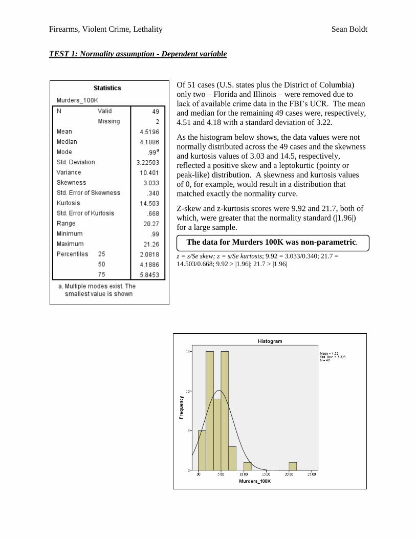
TEST 1: Normality assumption - Dependent variable
Of 51 cases (U.S. states plus the District of Columbia)
only two – Florida and Illinois – were removed due to
lack of available crime data in the FBI’s UCR. The mean
and median for the remaining 49 cases were, respectively,
4.51 and 4.18 with a standard deviation of 3.22.
As the histogram below shows, the data values were not
normally distributed across the 49 cases and the skewness
and kurtosis values of 3.03 and 14.5, respectively,
reflected a positive skew and a leptokurtic (pointy or
peak-like) distribution. A skewness and kurtosis values
of 0, for example, would result in a distribution that
matched exactly the normality curve.
Z-skew and z-kurtosis scores were 9.92 and 21.7, both of
which, were greater that the normality standard (|1.96|)
for a large sample.
The data for Murders 100K was non-parametric.
z = s/Se skew; z = s/Se kurtosis; 9.92 = 3.033/0.340; 21.7 =
14.503/0.668; 9.92 > |1.96|; 21.7 > |1.96|
Firearms, Violent Crime, Lethality Sean Boldt
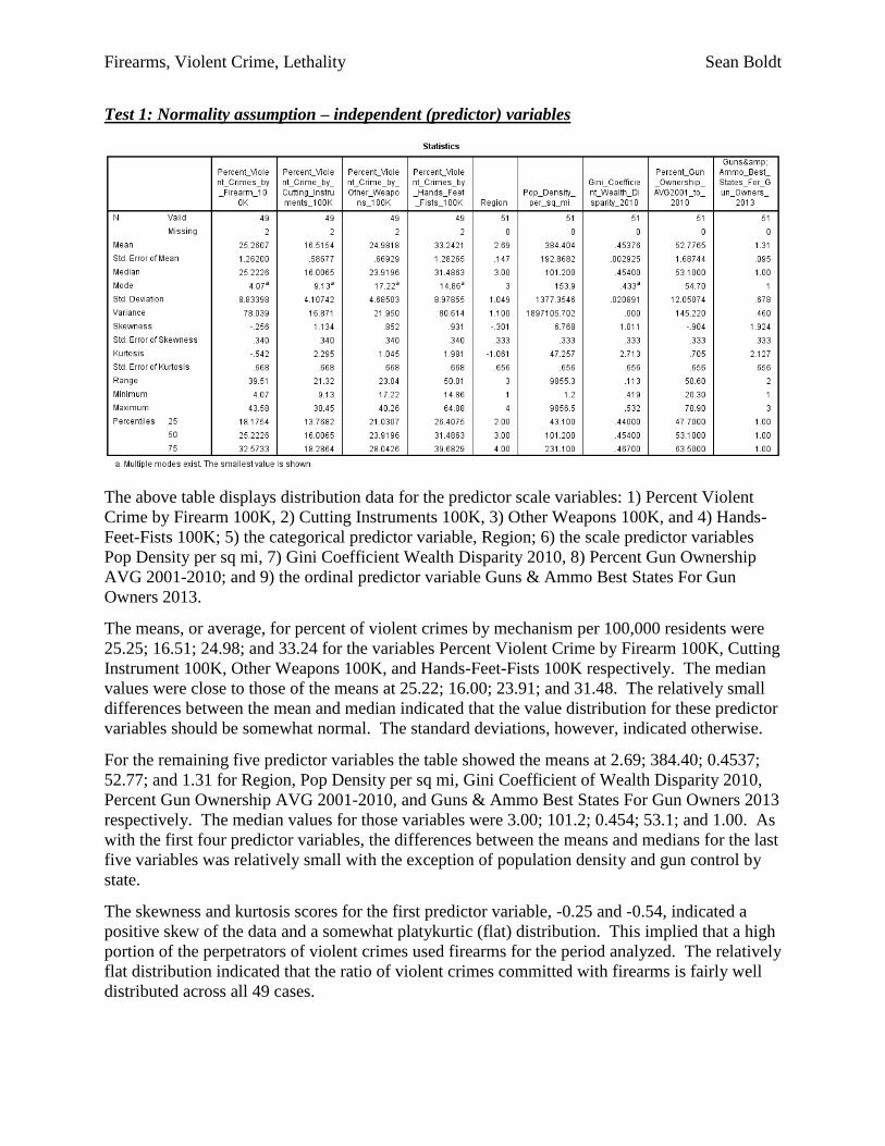
Test 1: Normality assumption – independent (predictor) variables
The above table displays distribution data for the predictor scale variables: 1) Percent Violent
Crime by Firearm 100K, 2) Cutting Instruments 100K, 3) Other Weapons 100K, and 4) Hands-
Feet-Fists 100K; 5) the categorical predictor variable, Region; 6) the scale predictor variables
Pop Density per sq mi, 7) Gini Coefficient Wealth Disparity 2010, 8) Percent Gun Ownership
AVG 2001-2010; and 9) the ordinal predictor variable Guns & Ammo Best States For Gun
Owners 2013.
The means, or average, for percent of violent crimes by mechanism per 100,000 residents were
25.25; 16.51; 24.98; and 33.24 for the variables Percent Violent Crime by Firearm 100K, Cutting
Instrument 100K, Other Weapons 100K, and Hands-Feet-Fists 100K respectively. The median
values were close to those of the means at 25.22; 16.00; 23.91; and 31.48. The relatively small
differences between the mean and median indicated that the value distribution for these predictor
variables should be somewhat normal. The standard deviations, however, indicated otherwise.
For the remaining five predictor variables the table showed the means at 2.69; 384.40; 0.4537;
52.77; and 1.31 for Region, Pop Density per sq mi, Gini Coefficient of Wealth Disparity 2010,
Percent Gun Ownership AVG 2001-2010, and Guns & Ammo Best States For Gun Owners 2013
respectively. The median values for those variables were 3.00; 101.2; 0.454; 53.1; and 1.00. As
with the first four predictor variables, the differences between the means and medians for the last
five variables was relatively small with the exception of population density and gun control by
state.
The skewness and kurtosis scores for the first predictor variable, -0.25 and -0.54, indicated a
positive skew of the data and a somewhat platykurtic (flat) distribution. This implied that a high
portion of the perpetrators of violent crimes used firearms for the period analyzed. The relatively
flat distribution indicated that the ratio of violent crimes committed with firearms is fairly well
distributed across all 49 cases.
Firearms, Violent Crime, Lethality Sean Boldt
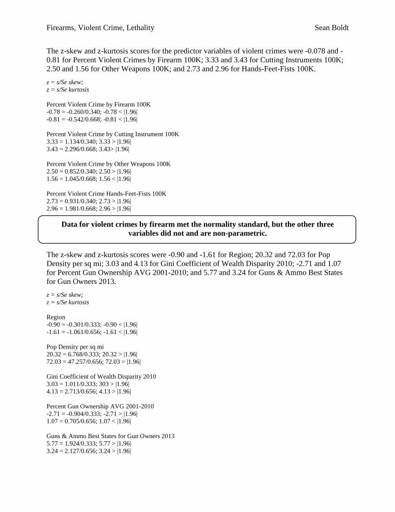
The z-skew and z-kurtosis scores for the predictor variables of violent crimes were -0.078 and -
0.81 for Percent Violent Crimes by Firearm 100K; 3.33 and 3.43 for Cutting Instruments 100K;
2.50 and 1.56 for Other Weapons 100K; and 2.73 and 2.96 for Hands-Feet-Fists 100K.
z = s/Se skew;
z = s/Se kurtosis
Percent Violent Crime by Firearm 100K
-0.78 = -0.260/0.340; -0.78 < |1.96|
-0.81 = -0.542/0.668; -0.81 < |1.96|
Percent Violent Crime by Cutting Instrument 100K
3.33 = 1.134/0.340; 3.33 > |1.96|
3.43 = 2.296/0.668; 3.43> |1.96|
Percent Violent Crime by Other Weapons 100K
2.50 = 0.852/0.340; 2.50 > |1.96|
1.56 = 1.045/0.668; 1.56 < |1.96|
Percent Violent Crime Hands-Feet-Fists 100K
2.73 = 0.931/0.340; 2.73 > |1.96|
2.96 = 1.981/0.668; 2.96 > |1.96|
Data for violent crimes by firearm met the normality standard, but the other three
variables did not and are non-parametric.
The z-skew and z-kurtosis scores were -0.90 and -1.61 for Region; 20.32 and 72.03 for Pop
Density per sq mi; 3.03 and 4.13 for Gini Coefficient of Wealth Disparity 2010; -2.71 and 1.07
for Percent Gun Ownership AVG 2001-2010; and 5.77 and 3.24 for Guns & Ammo Best States
for Gun Owners 2013.
z = s/Se skew;
z = s/Se kurtosis
Region
-0.90 = -0.301/0.333; -0.90 < |1.96|
-1.61 = -1.061/0.656; -1.61 < |1.96|
Pop Density per sq mi
20.32 = 6.768/0.333; 20.32 > |1.96|
72.03 = 47.257/0.656; 72.03 > |1.96|
Gini Coefficient of Wealth Disparity 2010
3.03 = 1.011/0.333; 303 > |1.96|
4.13 = 2.713/0.656; 4.13 > |1.96|
Percent Gun Ownership AVG 2001-2010
-2.71 = -0.904/0.333; -2.71 > |1.96|
1.07 = 0.705/0.656; 1.07 < |1.96|
Guns & Ammo Best States for Gun Owners 2013
5.77 = 1.924/0.333; 5.77 > |1.96|
3.24 = 2.127/0.656; 3.24 > |1.96|
Firearms, Violent Crime, Lethality Sean Boldt
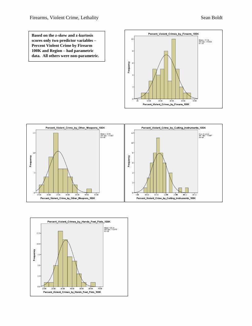
Based on the z-skew and z-kurtosis
scores only two predictor variables –
Percent Violent Crime by Firearm
100K and Region – had parametric
data. All others were non-parametric.
Firearms, Violent Crime, Lethality Sean Boldt
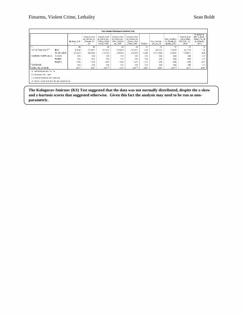
The Kologorav-Smirnov (KS) Test suggested that the data was not normally distributed, despite the z-skew
and z-kurtosis scores that suggested otherwise. Given this fact the analysis may need to be run as non-
parametric.
Firearms, Violent Crime, Lethality Sean Boldt
Test 2: Outliers
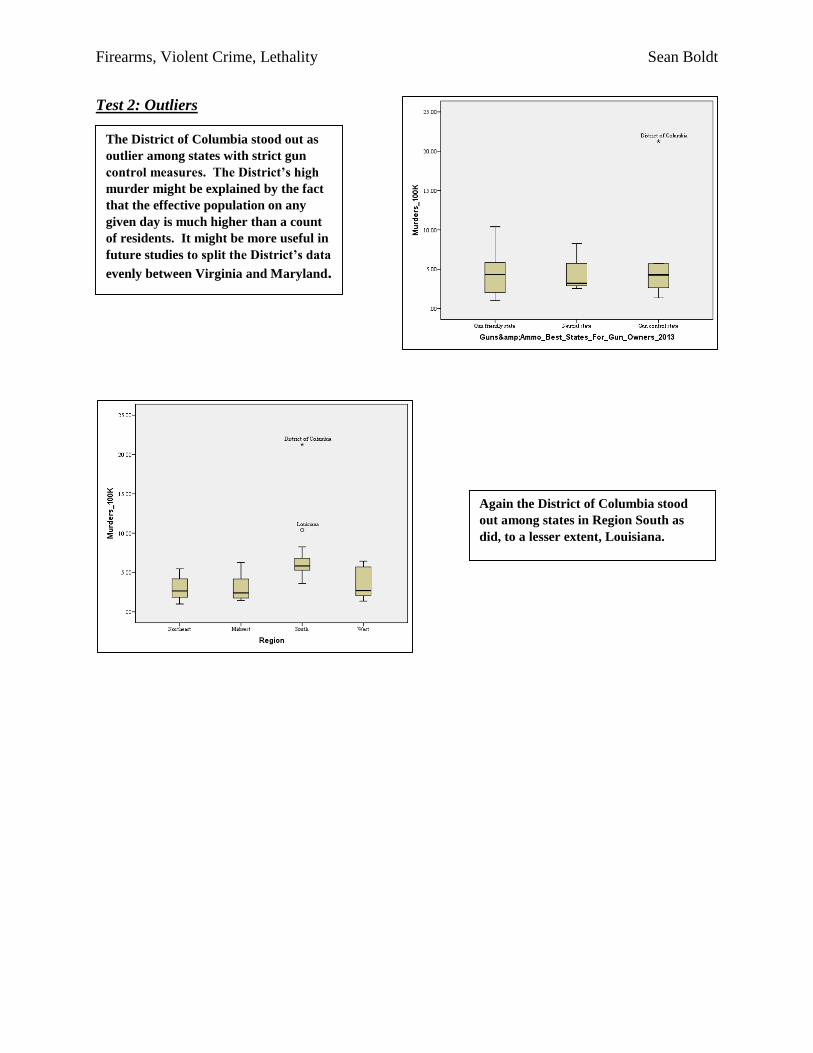
The District of Columbia stood out as
outlier among states with strict gun
control measures. The District’s high
murder might be explained by the fact
that the effective population on any
given day is much higher than a count
of residents. It might be more useful in
future studies to split the District’s data
evenly between Virginia and Maryland.
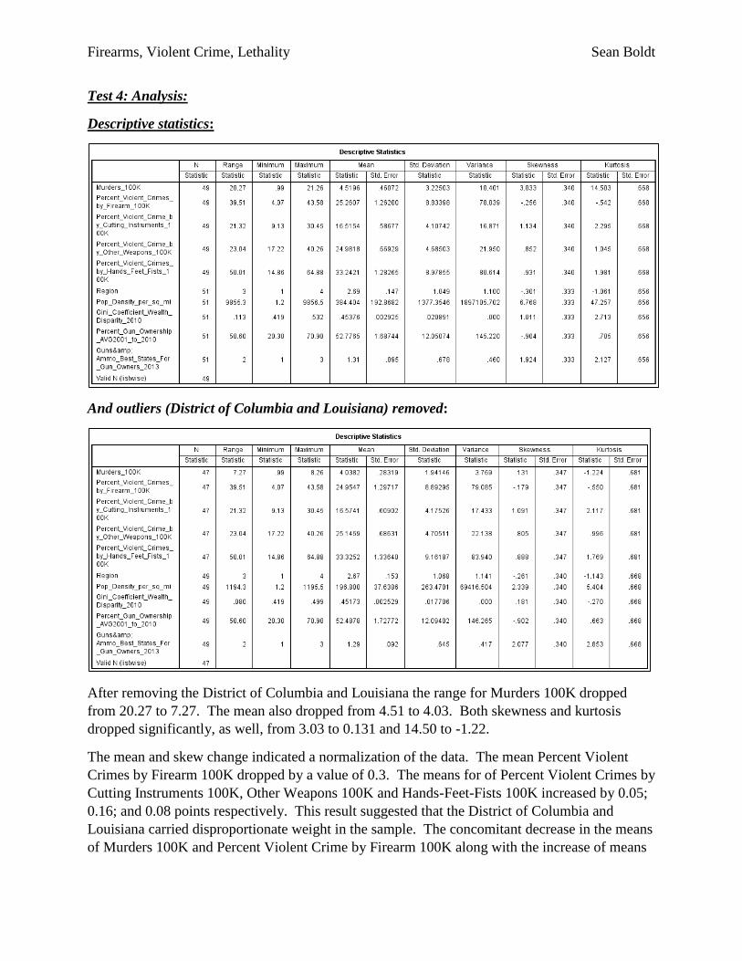
Again the District of Columbia stood
out among states in Region South as
did, to a lesser extent, Louisiana.
Firearms, Violent Crime, Lethality Sean Boldt
Test 4: Analysis:
Descriptive statistics:
And outliers (District of Columbia and Louisiana) removed:
After removing the District of Columbia and Louisiana the range for Murders 100K dropped
from 20.27 to 7.27. The mean also dropped from 4.51 to 4.03. Both skewness and kurtosis
dropped significantly, as well, from 3.03 to 0.131 and 14.50 to -1.22.
The mean and skew change indicated a normalization of the data. The mean Percent Violent
Crimes by Firearm 100K dropped by a value of 0.3. The means for of Percent Violent Crimes by
Cutting Instruments 100K, Other Weapons 100K and Hands-Feet-Fists 100K increased by 0.05;
0.16; and 0.08 points respectively. This result suggested that the District of Columbia and
Louisiana carried disproportionate weight in the sample. The concomitant decrease in the means
of Murders 100K and Percent Violent Crime by Firearm 100K along with the increase of means
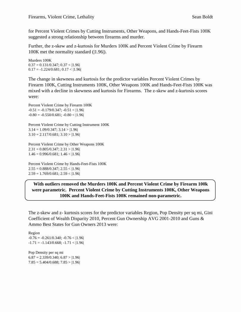
Firearms, Violent Crime, Lethality Sean Boldt
for Percent Violent Crimes by Cutting Instruments, Other Weapons, and Hands-Feet-Fists 100K
suggested a strong relationship between firearms and murder.
Further, the z-skew and z-kurtosis for Murders 100K and Percent Violent Crime by Firearm
100K met the normality standard (|1.96|).
Murders 100K
0.37 = 0.131/0.347; 0.37 < |1.96|
0.17 = -1.224/0.681; 0.17 < |1.96|
The change in skewness and kurtosis for the predictor variables Percent Violent Crimes by
Firearm 100K, Cutting Instruments 100K, Other Weapons 100K and Hands-Feet-Fists 100K was
mixed with a decline in skewness and kurtosis for Firearms. The z-skew and z-kurtosis scores
were:
Percent Violent Crime by Firearm 100K
-0.51 = -0.179/0.347; -0.51 < |1.96|
-0.80 = -0.550/0.681; -0.80 < |1.96|
Percent Violent Crime by Cutting Instrument 100K
3.14 = 1.09/0.347; 3.14 > |1.96|
3.10 = 2.117/0.681; 3.10 > |1.96|
Percent Violent Crime by Other Weapons 100K
2.31 = 0.805/0.347; 2.31 > |1.96|
1.46 = 0.996/0.681; 1.46 < |1.96|
Percent Violent Crime by Hands-Feet-Fists 100K
2.55 = 0.888/0.347; 2.55 < |1.96|
2.59 = 1.769/0.681; 2.59 < |1.96|
With outliers removed the Murders 100K and Percent Violent Crime by Firearm 100k
were parametric. Percent Violent Crime by Cutting Instruments 100K, Other Weapons
100K and Hands-Feet-Fists 100K remained non-parametric.
The z-skew and z- kurtosis scores for the predictor variables Region, Pop Density per sq mi, Gini
Coefficient of Wealth Disparity 2010, Percent Gun Ownership AVG 2001-2010 and Guns &
Ammo Best States for Gun Owners 2013 were:
Region
-0.76 = -0.261/0.340; -0.76 < |1.96|
-1.71 = -1.143/0.668; -1.71 < |1.96|
Pop Density per sq mi
6.87 = 2.339/0.340; 6.87 > |1.96|
7.85 = 5.404/0.688; 7.85 > |1.96|
Firearms, Violent Crime, Lethality Sean Boldt
Gini Coefficient of Wealth Disparity 2010
0.53 = 0.181/0.340; 0.53 < |1.96|
-0.40 = -0.270/0.668; -0.40 < |1.96|
Percent Gun Ownership AVG 2001-2010
-2.65 = -0.902/0.340; -2.65 > |1.96|
0.99 = 0.663/0.668; 0.99 < |1.96|
Guns & Ammo Best States for Gun Owners 2013
6.10 = 2.077/0.340; 6.10 > |1.96|
4.27 = 2.853/0.668; 4.27 > |1.96|
Region and Gini Coefficient of Wealth Disparity 2010 were normal, or parametric. All
others were non-parametric.
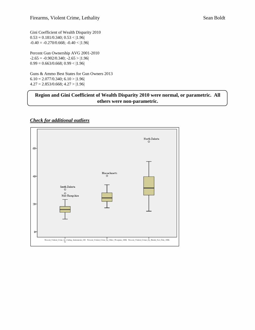
Check for additional outliers
Firearms, Violent Crime, Lethality Sean Boldt
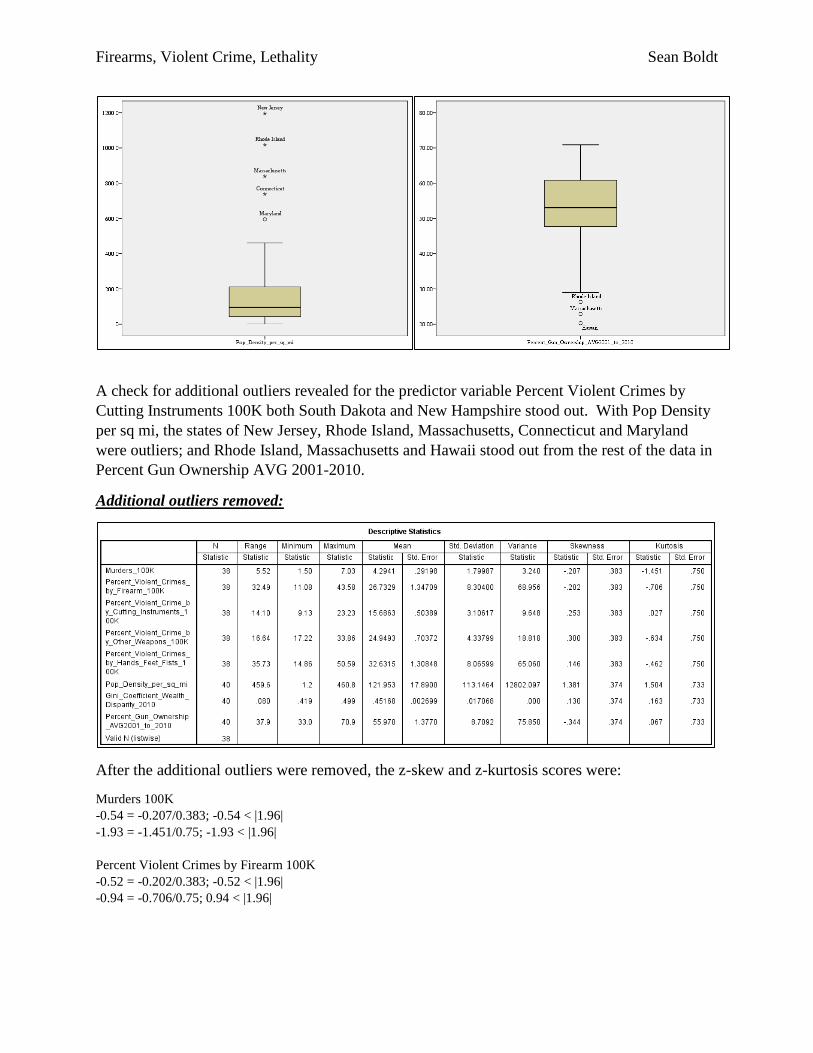
A check for additional outliers revealed for the predictor variable Percent Violent Crimes by
Cutting Instruments 100K both South Dakota and New Hampshire stood out. With Pop Density
per sq mi, the states of New Jersey, Rhode Island, Massachusetts, Connecticut and Maryland
were outliers; and Rhode Island, Massachusetts and Hawaii stood out from the rest of the data in
Percent Gun Ownership AVG 2001-2010.
Additional outliers removed:
After the additional outliers were removed, the z-skew and z-kurtosis scores were:
Murders 100K
-0.54 = -0.207/0.383; -0.54 < |1.96|
-1.93 = -1.451/0.75; -1.93 < |1.96|
Percent Violent Crimes by Firearm 100K
-0.52 = -0.202/0.383; -0.52 < |1.96|
-0.94 = -0.706/0.75; 0.94 < |1.96|
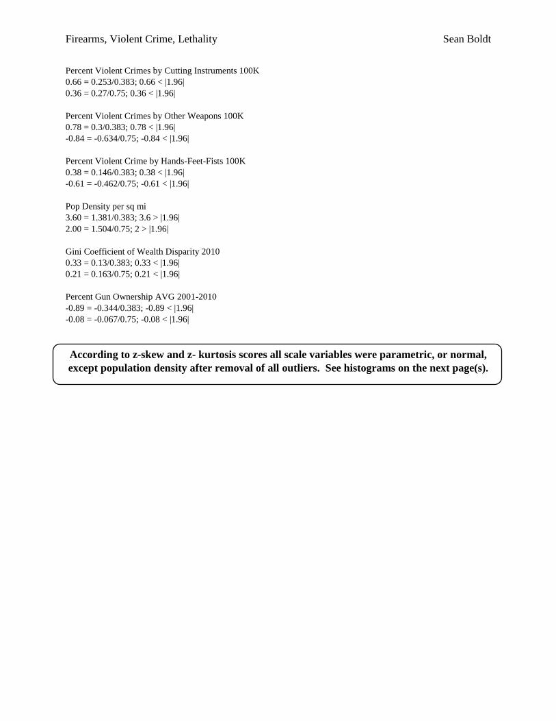
Firearms, Violent Crime, Lethality Sean Boldt
Percent Violent Crimes by Cutting Instruments 100K
0.66 = 0.253/0.383; 0.66 < |1.96|
0.36 = 0.27/0.75; 0.36 < |1.96|
Percent Violent Crimes by Other Weapons 100K
0.78 = 0.3/0.383; 0.78 < |1.96|
-0.84 = -0.634/0.75; -0.84 < |1.96|
Percent Violent Crime by Hands-Feet-Fists 100K
0.38 = 0.146/0.383; 0.38 < |1.96|
-0.61 = -0.462/0.75; -0.61 < |1.96|
Pop Density per sq mi
3.60 = 1.381/0.383; 3.6 > |1.96|
2.00 = 1.504/0.75; 2 > |1.96|
Gini Coefficient of Wealth Disparity 2010
0.33 = 0.13/0.383; 0.33 < |1.96|
0.21 = 0.163/0.75; 0.21 < |1.96|
Percent Gun Ownership AVG 2001-2010
-0.89 = -0.344/0.383; -0.89 < |1.96|
-0.08 = -0.067/0.75; -0.08 < |1.96|
According to z-skew and z- kurtosis scores all scale variables were parametric, or normal,
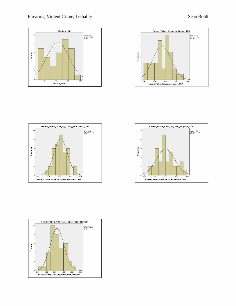
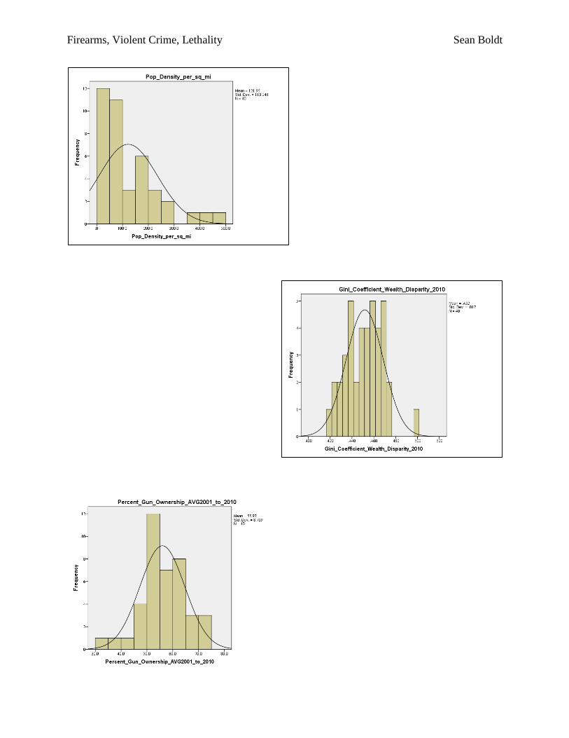
except population density after removal of all outliers. See histograms on the next page(s).
Firearms, Violent Crime, Lethality Sean Boldt
Firearms, Violent Crime, Lethality Sean Boldt
Firearms, Violent Crime, Lethality Sean Boldt
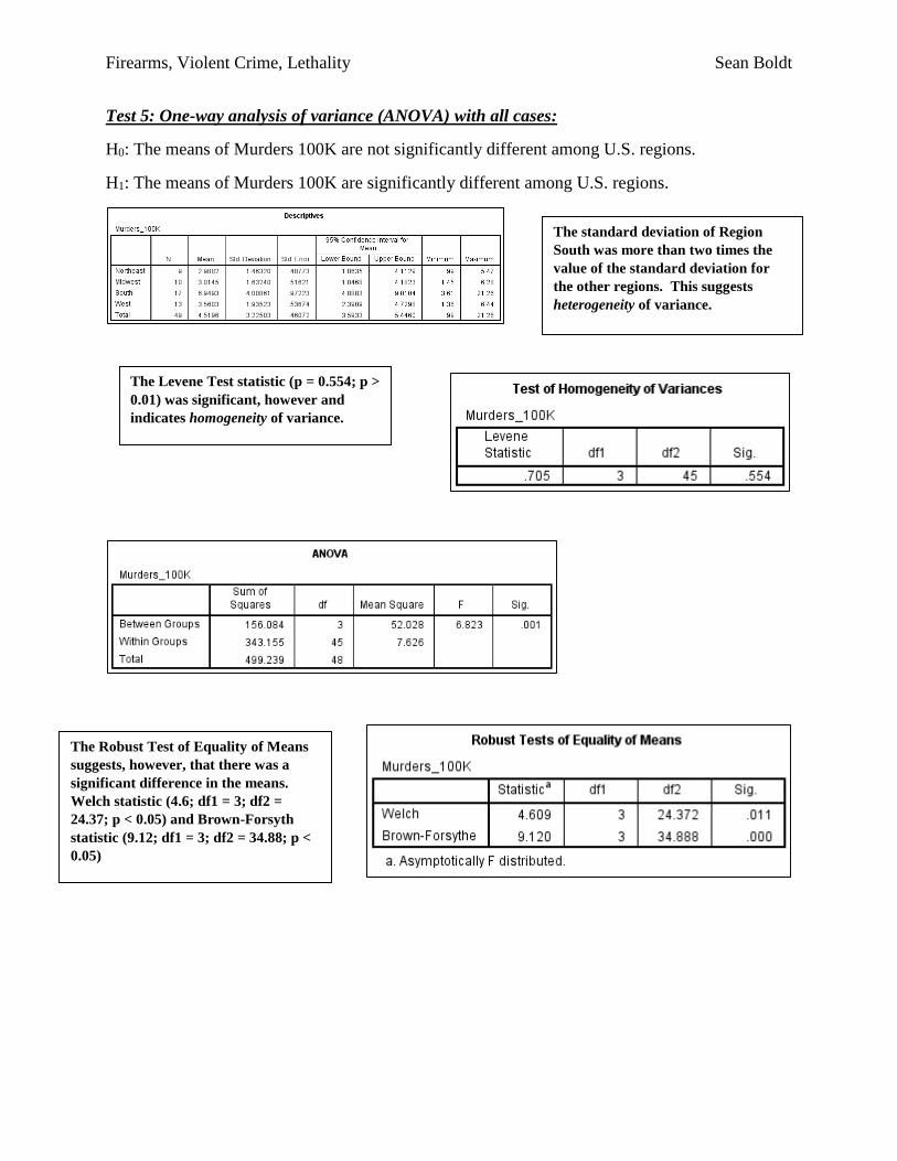
Test 5: One-way analysis of variance (ANOVA) with all cases:
H0: The means of Murders 100K are not significantly different among U.S. regions.
H1: The means of Murders 100K are significantly different among U.S. regions.
The standard deviation of Region
South was more than two times the
value of the standard deviation for
the other regions. This suggests
heterogeneity of variance.
The Levene Test statistic (p = 0.554; p >
0.01) was significant, however and
indicates homogeneity of variance.
The Robust Test of Equality of Means
suggests, however, that there was a
significant difference in the means.
Welch statistic (4.6; df1 = 3; df2 =
24.37; p < 0.05) and Brown-Forsyth
statistic (9.12; df1 = 3; df2 = 34.88; p <
0.05)
Firearms, Violent Crime, Lethality Sean Boldt
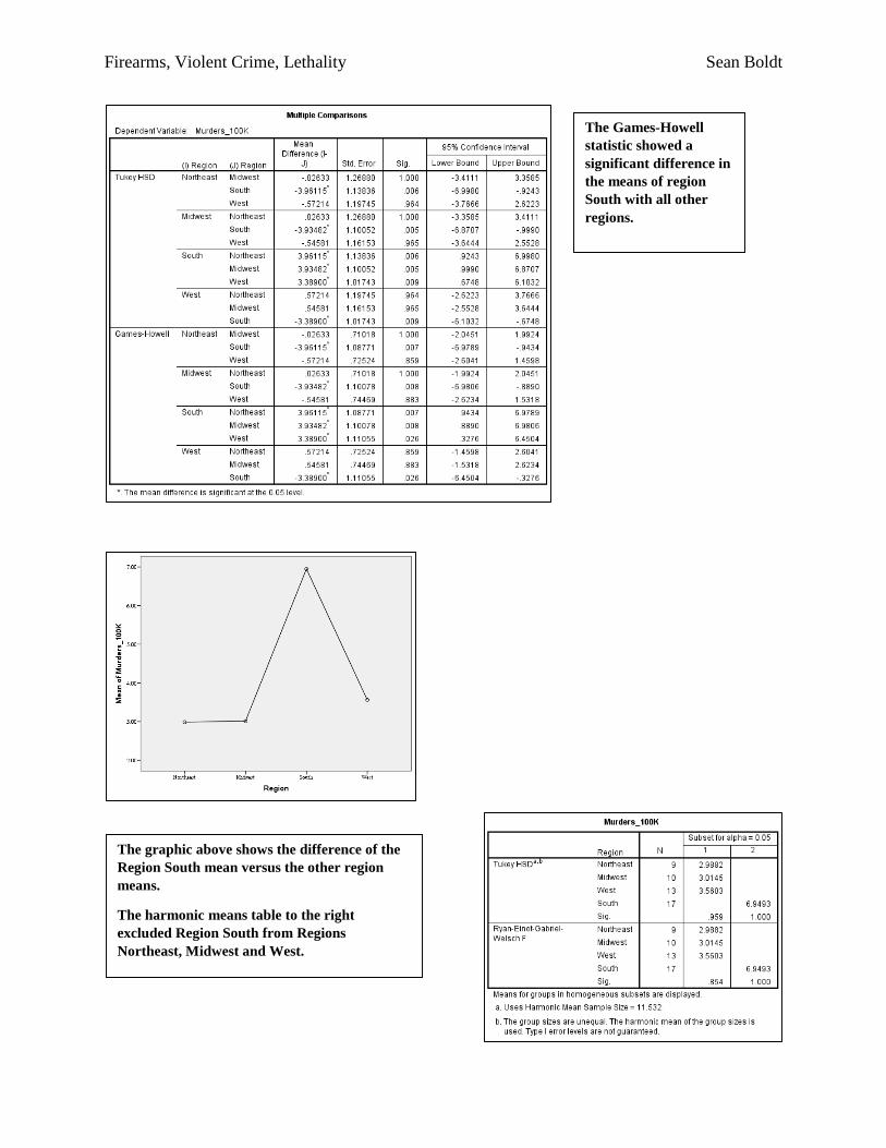
The Games-Howell
statistic showed a
significant difference in
the means of region
South with all other
regions.
The graphic above shows the difference of the
Region South mean versus the other region
means.
The harmonic means table to the right
excluded Region South from Regions
Northeast, Midwest and West.
Firearms, Violent Crime, Lethality Sean Boldt
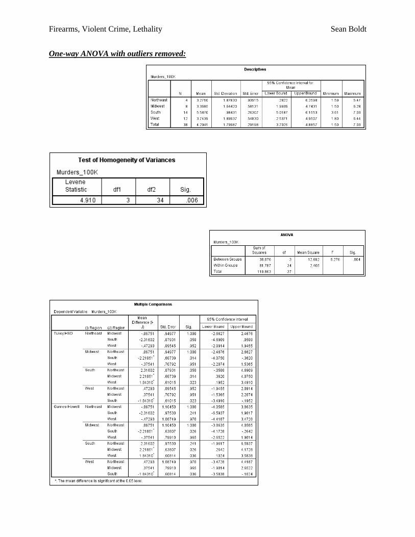
One-way ANOVA with outliers removed:
Firearms, Violent Crime, Lethality Sean Boldt
The same conclusion was reached without outliers as was with the outliers. The null
hypothesis is rejected, the alternative hypothesis as assumed - there is significant
difference in the means of rate of murder for the four U.S. regions.
Firearms, Violent Crime, Lethality Sean Boldt
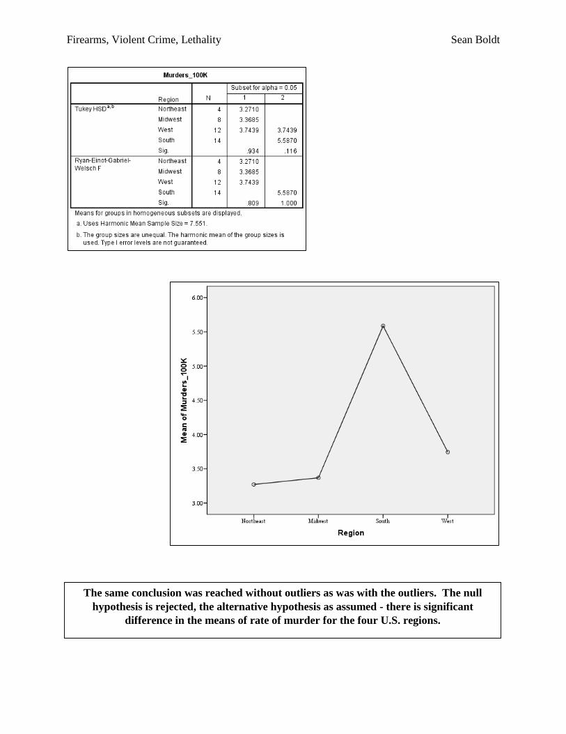
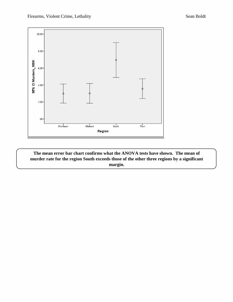
The mean error bar chart confirms what the ANOVA tests have shown. The mean of
murder rate for the region South exceeds those of the other three regions by a significant
margin.
Firearms, Violent Crime, Lethality Sean Boldt
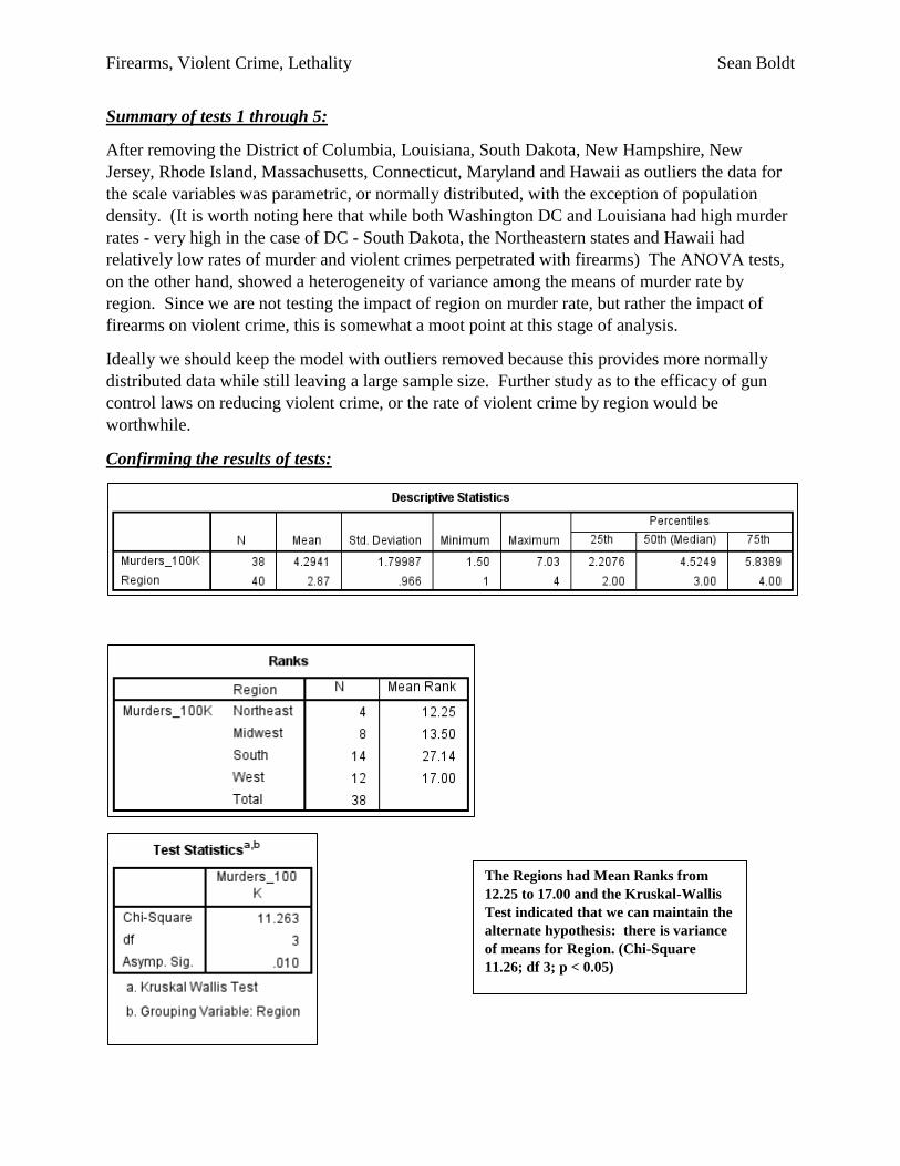
Summary of tests 1 through 5:
After removing the District of Columbia, Louisiana, South Dakota, New Hampshire, New
Jersey, Rhode Island, Massachusetts, Connecticut, Maryland and Hawaii as outliers the data for
the scale variables was parametric, or normally distributed, with the exception of population
density. (It is worth noting here that while both Washington DC and Louisiana had high murder
rates - very high in the case of DC - South Dakota, the Northeastern states and Hawaii had
relatively low rates of murder and violent crimes perpetrated with firearms) The ANOVA tests,
on the other hand, showed a heterogeneity of variance among the means of murder rate by
region. Since we are not testing the impact of region on murder rate, but rather the impact of
firearms on violent crime, this is somewhat a moot point at this stage of analysis.
Ideally we should keep the model with outliers removed because this provides more normally
distributed data while still leaving a large sample size. Further study as to the efficacy of gun
control laws on reducing violent crime, or the rate of violent crime by region would be
worthwhile.
Confirming the results of tests:
The Regions had Mean Ranks from
12.25 to 17.00 and the Kruskal-Wallis
Test indicated that we can maintain the
alternate hypothesis: there is variance
of means for Region. (Chi-Square
11.26; df 3; p < 0.05)
Firearms, Violent Crime, Lethality Sean Boldt
Multiple Regression:
Hypotheses:
H0: The type of weapon used in the commission of a violent crime will not predict the U.S.
murder rate more accurately than the mean.
H1: The use of a firearm in the commission of a violent crime will predict the U.S. murder rate
more accurately than the mean.
H2: The use of a cutting instrument in the commission of a violent crime will predict the U.S.
murder rate more accurately than the mean.
H3: The use of other weapons in the commission of a violent crime will predict the U.S. murder
rate more accurately than the mean.
H4: The use of hands-feet-fists in the commission of a violent crime will predict the U.S. murder
rate more accurately than the mean.
H5: Region will predict the U.S. murder rate more accurately than the mean.
H6: Population density will predict the U.S. murder rate more accurately than the mean.
H7: The Gini Coefficient of Wealth Disparity will predict the U.S. murder rate more accurately
than the mean.
H8: The percentage of gun ownership will predict the U.S. murder rate more accurately than the
mean.
H9: State gun friendliness will predict the U.S. murder rate more accurately than the mean.
H10: Any combination of the above predictor variables will predict the U.S. murder rate more
accurately than the mean.
Firearms, Violent Crime, Lethality Sean Boldt
Correlations:
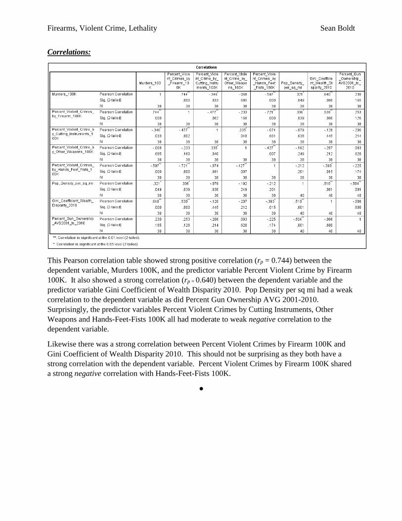
This Pearson correlation table showed strong positive correlation (rp = 0.744) between the
dependent variable, Murders 100K, and the predictor variable Percent Violent Crime by Firearm
100K. It also showed a strong correlation (rp = 0.640) between the dependent variable and the
predictor variable Gini Coefficient of Wealth Disparity 2010. Pop Density per sq mi had a weak
correlation to the dependent variable as did Percent Gun Ownership AVG 2001-2010.
Surprisingly, the predictor variables Percent Violent Crimes by Cutting Instruments, Other
Weapons and Hands-Feet-Fists 100K all had moderate to weak negative correlation to the
dependent variable.
Likewise there was a strong correlation between Percent Violent Crimes by Firearm 100K and
Gini Coefficient of Wealth Disparity 2010. This should not be surprising as they both have a
strong correlation with the dependent variable. Percent Violent Crimes by Firearm 100K shared
a strong negative correlation with Hands-Feet-Fists 100K.
●
Firearms, Violent Crime, Lethality Sean Boldt
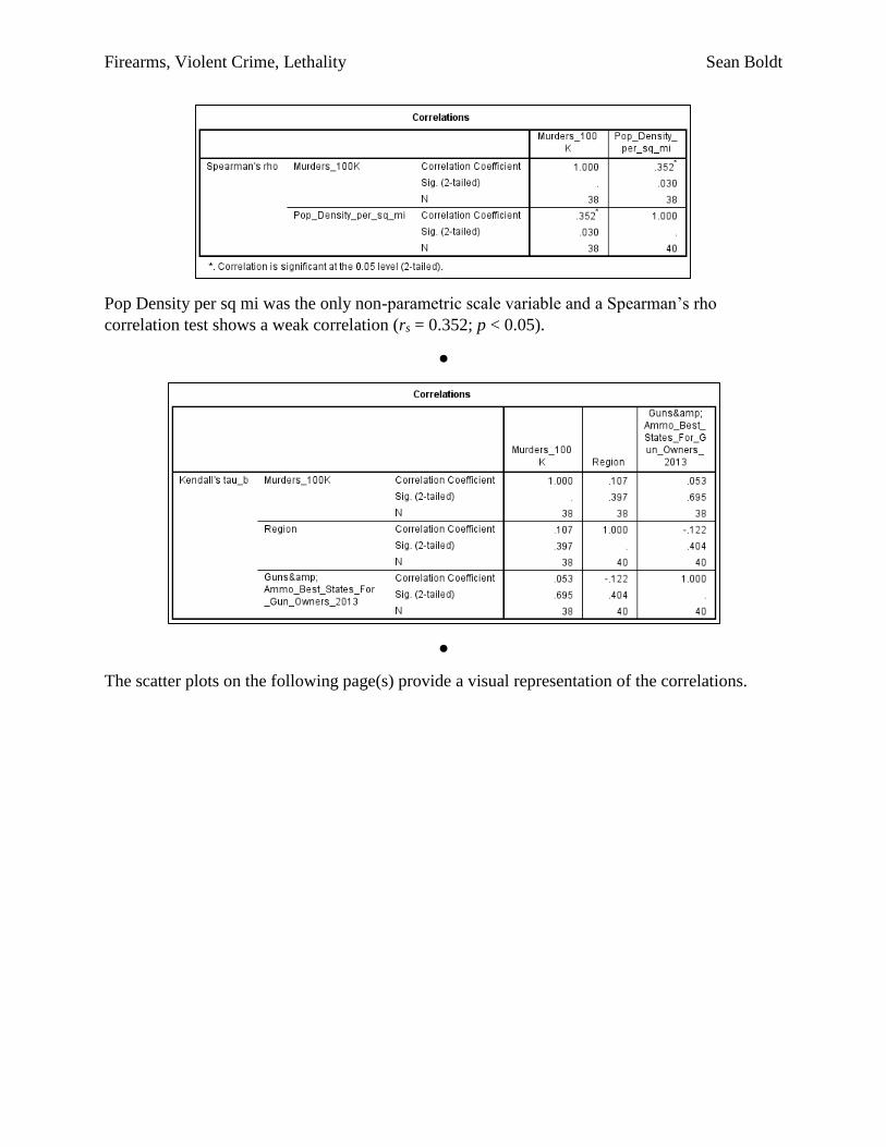
Pop Density per sq mi was the only non-parametric scale variable and a Spearman’s rho
correlation test shows a weak correlation (rs = 0.352; p < 0.05).
●
●
The scatter plots on the following page(s) provide a visual representation of the correlations.
Firearms, Violent Crime, Lethality Sean Boldt
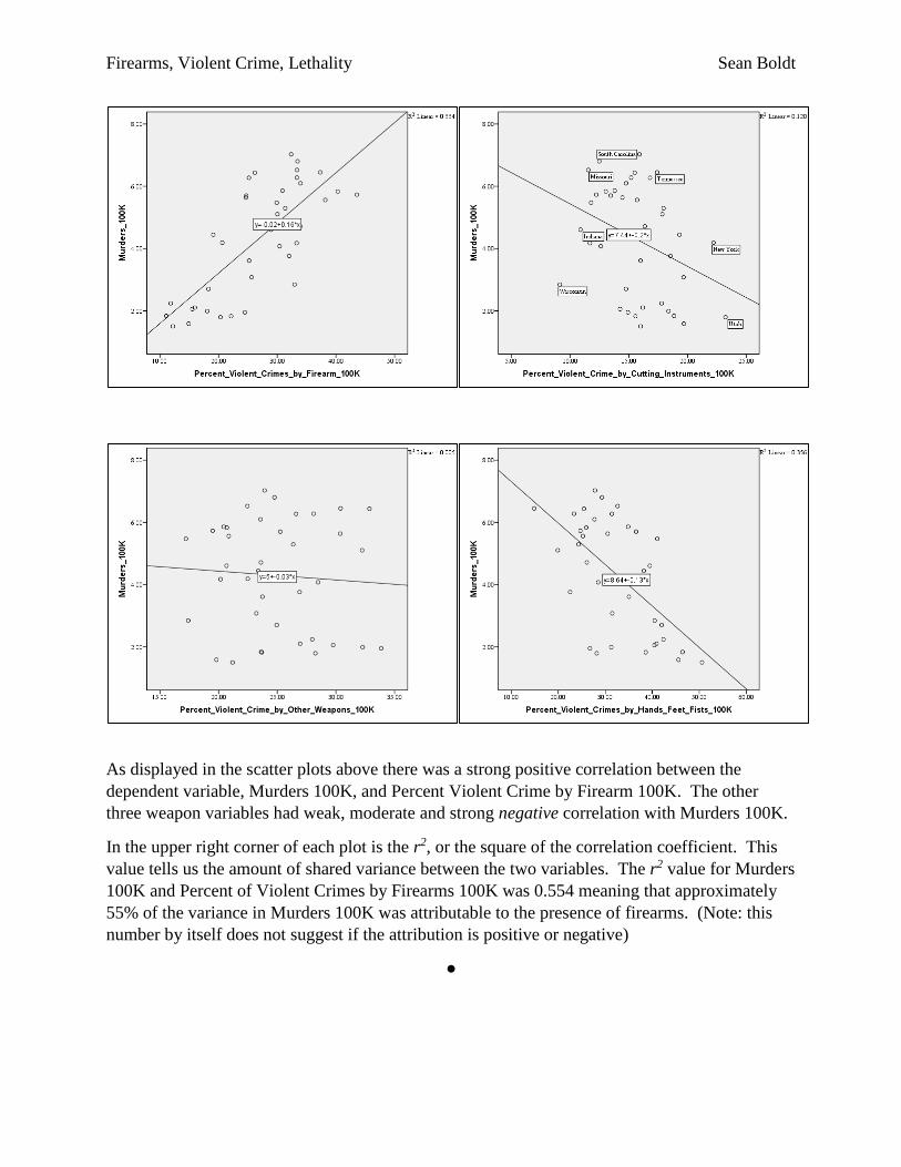
As displayed in the scatter plots above there was a strong positive correlation between the
dependent variable, Murders 100K, and Percent Violent Crime by Firearm 100K. The other
three weapon variables had weak, moderate and strong negative correlation with Murders 100K.
In the upper right corner of each plot is the r2, or the square of the correlation coefficient. This
value tells us the amount of shared variance between the two variables. The r2 value for Murders
100K and Percent of Violent Crimes by Firearms 100K was 0.554 meaning that approximately
55% of the variance in Murders 100K was attributable to the presence of firearms. (Note: this
number by itself does not suggest if the attribution is positive or negative)
●
Firearms, Violent Crime, Lethality Sean Boldt
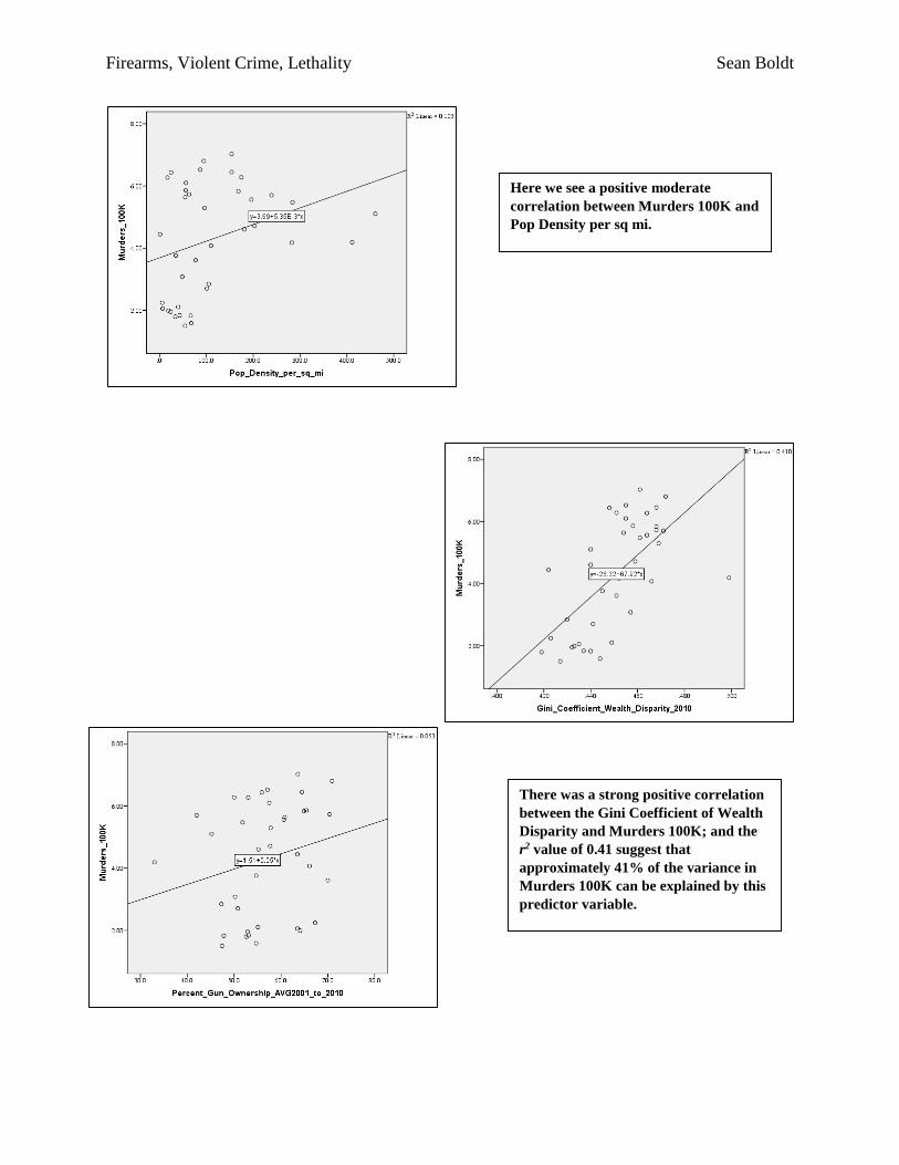
Here we see a positive moderate
correlation between Murders 100K and
Pop Density per sq mi.
There was a strong positive correlation
between the Gini Coefficient of Wealth
Disparity and Murders 100K; and the
r2 value of 0.41 suggest that
approximately 41% of the variance in
Murders 100K can be explained by this
predictor variable.
Firearms, Violent Crime, Lethality Sean Boldt
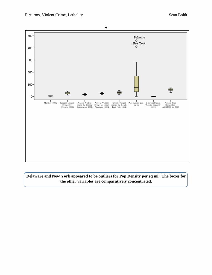
●
Delaware and New York appeared to be outliers for Pop Density per sq mi. The boxes for
the other variables are comparatively concentrated.
Firearms, Violent Crime, Lethality Sean Boldt
Stepwise regression:
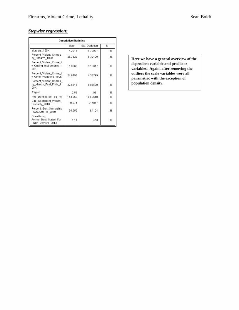
Here we have a general overview of the
dependent variable and predictor
variables. Again, after removing the
outliers the scale variables were all
parametric with the exception of
population density.
Firearms, Violent Crime, Lethality Sean Boldt
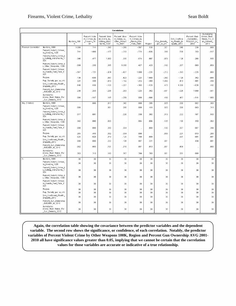
Again, the correlation table showing the covariance between the predictor variables and the dependent
variable. The second row shows the significance, or confidence, of each correlation. Notably, the predictor
variables of Percent Violent Crime by Other Weapons 100K, Region and Percent Gun Ownership AVG 2001-
2010 all have significance values greater than 0.05, implying that we cannot be certain that the correlation
values for those variables are accurate or indicative of a true relationship.
Firearms, Violent Crime, Lethality Sean Boldt
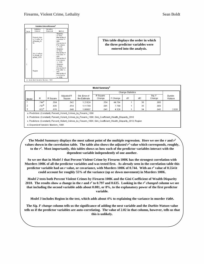
The Model Summary displays the most salient point of the multiple regression. Here we see the r and r2
values shown in the correlation table. The table also shows the adjusted r2 value which corresponds, roughly,
to the r2. Most importantly, this tables shows us how each of the predictor variables interact with the
dependent variable independently of one another.
So we see that in Model 1 that Percent Violent Crime by Firearm 100K has the strongest correlation with
Murders 100K of all the predictor variables and was tested first. As already seen in the correlation table this
predictor variable had an r value, or covariance, with Murders 100K of 0.744. With an r2 value of 0.554 it
could account for roughly 55% of the variance (up or down movement) in Murders 100K.
Model 2 tests both Percent Violent Crimes by Firearm 100K and the Gini Coefficient of Wealth Disparity
2010. The results show a change in the r and r2 to 0.797 and 0.635. Looking in the r2 changed column we see
that including the second variable adds about 0.081, or 8%, to the explanatory power of the first predictor
variable.
Model 3 includes Region in the test, which adds about 4% to explaining the variance in murder rate.
The Sig. F change column tells us the significance of adding the next variable and the Durbin-Watson value
tells us if the predictor variables are auto-correlating. The value of 2.02 in that column, however, tells us that
this is unlikely.
This table displays the order in which
the three predictor variables were
entered into the analysis.
Firearms, Violent Crime, Lethality Sean Boldt
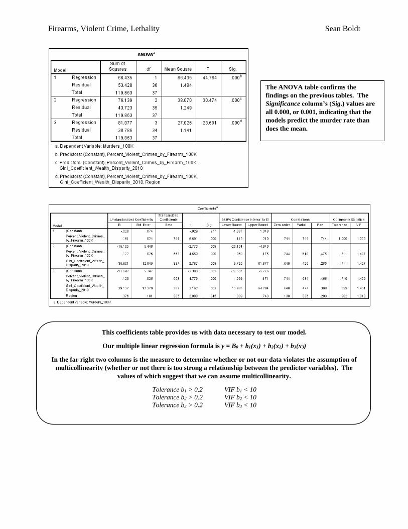
This coefficients table provides us with data necessary to test our model.
Our multiple linear regression formula is y = B0 + b1(x1) + b2(x2) + b3(x3)
In the far right two columns is the measure to determine whether or not our data violates the assumption of
multicollinearity (whether or not there is too strong a relationship between the predictor variables). The
values of which suggest that we can assume multicollinearity.
Tolerance b1 > 0.2 VIF b1 < 10
Tolerance b2 > 0.2 VIF b2 < 10
Tolerance b3 > 0.2 VIF b3 < 10
The ANOVA table confirms the
findings on the previous tables. The
Significance column’s (Sig.) values are
all 0.000, or 0.001, indicating that the
models predict the murder rate than
does the mean.
Firearms, Violent Crime, Lethality Sean Boldt
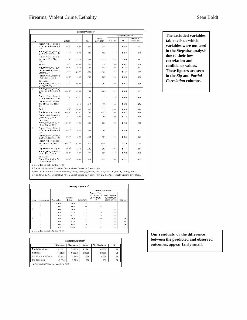
The excluded variables
table tells us which
variables were not used
in the Stepwise analysis
due to their low
correlation and
confidence values.
These figures are seen
in the Sig and Partial
Correlation columns.
Our residuals, or the difference
between the predicted and observed
outcomes, appear fairly small.
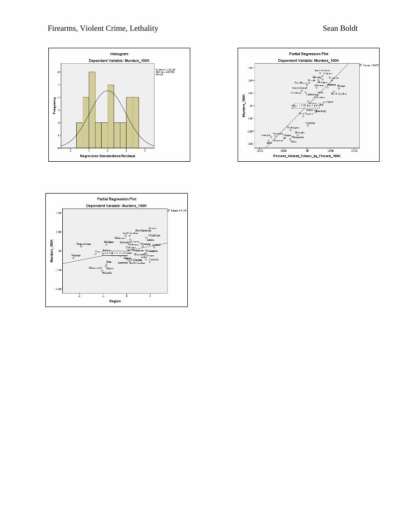
Firearms, Violent Crime, Lethality Sean Boldt
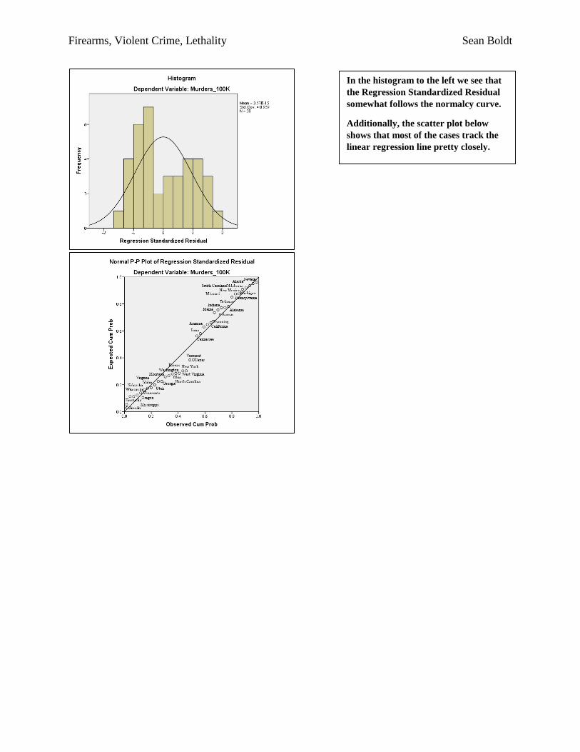
In the histogram to the left we see that
the Regression Standardized Residual
somewhat follows the normalcy curve.
Additionally, the scatter plot below
shows that most of the cases track the
linear regression line pretty closely.
Firearms, Violent Crime, Lethality Sean Boldt
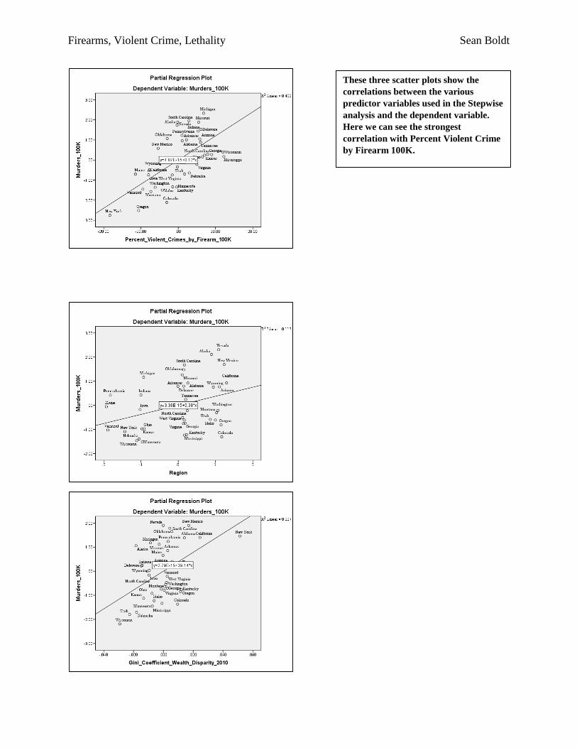
These three scatter plots show the
correlations between the various
predictor variables used in the Stepwise
analysis and the dependent variable.
Here we can see the strongest
correlation with Percent Violent Crime
by Firearm 100K.
Firearms, Violent Crime, Lethality Sean Boldt
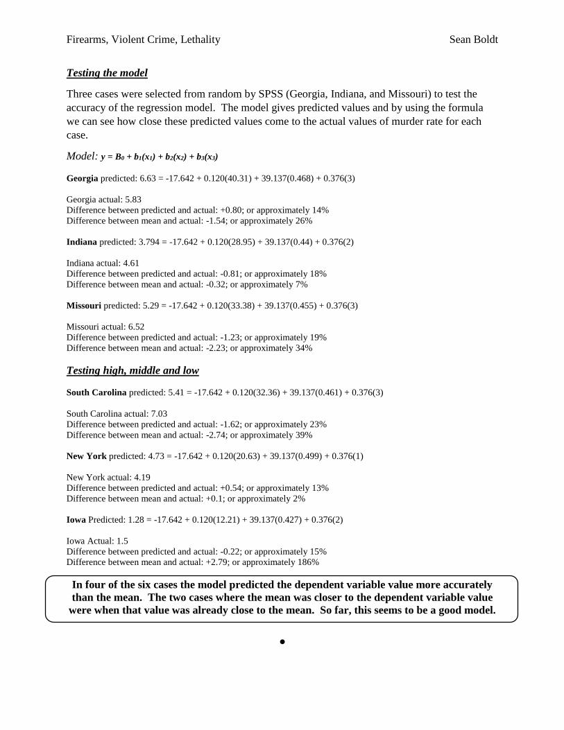
Testing the model
Three cases were selected from random by SPSS (Georgia, Indiana, and Missouri) to test the
accuracy of the regression model. The model gives predicted values and by using the formula
we can see how close these predicted values come to the actual values of murder rate for each
case.
Model: y = B0 + b1(x1) + b2(x2) + b3(x3)
Georgia predicted: 6.63 = -17.642 + 0.120(40.31) + 39.137(0.468) + 0.376(3)
Georgia actual: 5.83
Difference between predicted and actual: +0.80; or approximately 14%
Difference between mean and actual: -1.54; or approximately 26%
Indiana predicted: 3.794 = -17.642 + 0.120(28.95) + 39.137(0.44) + 0.376(2)
Indiana actual: 4.61
Difference between predicted and actual: -0.81; or approximately 18%
Difference between mean and actual: -0.32; or approximately 7%
Missouri predicted: 5.29 = -17.642 + 0.120(33.38) + 39.137(0.455) + 0.376(3)
Missouri actual: 6.52
Difference between predicted and actual: -1.23; or approximately 19%
Difference between mean and actual: -2.23; or approximately 34%
Testing high, middle and low
South Carolina predicted: 5.41 = -17.642 + 0.120(32.36) + 39.137(0.461) + 0.376(3)
South Carolina actual: 7.03
Difference between predicted and actual: -1.62; or approximately 23%
Difference between mean and actual: -2.74; or approximately 39%
New York predicted: 4.73 = -17.642 + 0.120(20.63) + 39.137(0.499) + 0.376(1)
New York actual: 4.19
Difference between predicted and actual: +0.54; or approximately 13%
Difference between mean and actual: +0.1; or approximately 2%
Iowa Predicted: 1.28 = -17.642 + 0.120(12.21) + 39.137(0.427) + 0.376(2)
Iowa Actual: 1.5
Difference between predicted and actual: -0.22; or approximately 15%
Difference between mean and actual: +2.79; or approximately 186%
In four of the six cases the model predicted the dependent variable value more accurately
than the mean. The two cases where the mean was closer to the dependent variable value
were when that value was already close to the mean. So far, this seems to be a good model.
●
Firearms, Violent Crime, Lethality Sean Boldt
Check for outliers:
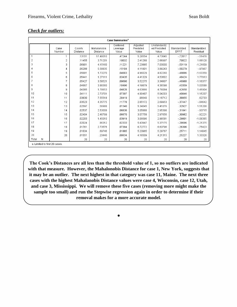
The Cook’s Distances are all less than the threshold value of 1, so no outliers are indicated
with that measure. However, the Mahalonobis Distance for case 1, New York, suggests that
it may be an outlier. The next highest in that category was case 11, Maine. The next three
cases with the highest Mahalanobis Distance values were case 4, Wisconsin, case 12, Utah,
and case 3, Mississippi. We will remove these five cases (removing more might make the
sample too small) and run the Stepwise regression again in order to determine if their
removal makes for a more accurate model.
●
Firearms, Violent Crime, Lethality Sean Boldt
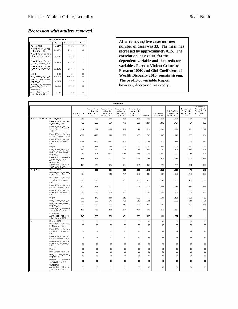
Regression with outliers removed:
After removing five cases our new
number of cases was 33. The mean has
increased by approximately 0.15. The
correlation, or r value, for the
dependent variable and the predictor
variables, Percent Violent Crime by
Firearm 100K and Gini Coefficient of
Wealth Disparity 2010, remain strong.
The predictor variable Region,
however, decreased markedly.
Firearms, Violent Crime, Lethality Sean Boldt
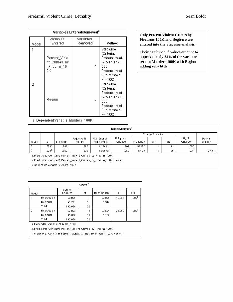
Only Percent Violent Crimes by
Firearms 100K and Region were
entered into the Stepwise analysis.
Their combined r2 values amount to
approximately 63% of the variance
seen in Murders 100K with Region
adding very little.
Firearms, Violent Crime, Lethality Sean Boldt
Firearms, Violent Crime, Lethality Sean Boldt
Firearms, Violent Crime, Lethality Sean Boldt
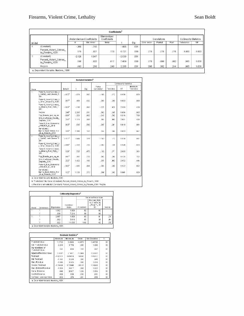
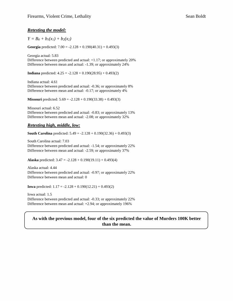
Retesting the model:
Y = B0 + b1(x1) + b2(x2)
Georgia predicted: 7.00 = -2.128 + 0.190(40.31) + 0.493(3)
Georgia actual: 5.83
Difference between predicted and actual: +1.17; or approximately 20%
Difference between mean and actual: -1.39; or approximately 24%
Indiana predicted: 4.25 = -2.128 + 0.190(28.95) + 0.493(2)
Indiana actual: 4.61
Difference between predicted and actual: -0.36; or approximately 8%
Difference between mean and actual: -0.17; or approximately 4%
Missouri predicted: 5.69 = -2.128 + 0.190(33.38) + 0.493(3)
Missouri actual: 6.52
Difference between predicted and actual: -0.83; or approximately 13%
Difference between mean and actual: -2.08; or approximately 32%
Retesting high, middle, low:
South Carolina predicted: 5.49 = -2.128 + 0.190(32.36) + 0.493(3)
South Carolina actual: 7.03
Difference between predicted and actual: -1.54; or approximately 22%
Difference between mean and actual: -2.59; or approximately 37%
Alaska predicted: 3.47 = -2.128 + 0.190(19.11) + 0.493(4)
Alaska actual: 4.44
Difference between predicted and actual: -0.97; or approximately 22%
Difference between mean and actual: 0
Iowa predicted: 1.17 = -2.128 + 0.190(12.21) + 0.493(2)
Iowa actual: 1.5
Difference between predicted and actual: -0.33; or approximately 22%
Difference between mean and actual: +2.94; or approximately 196%
As with the previous model, four of the six predicted the value of Murders 100K better
than the mean.
Firearms, Violent Crime, Lethality Sean Boldt
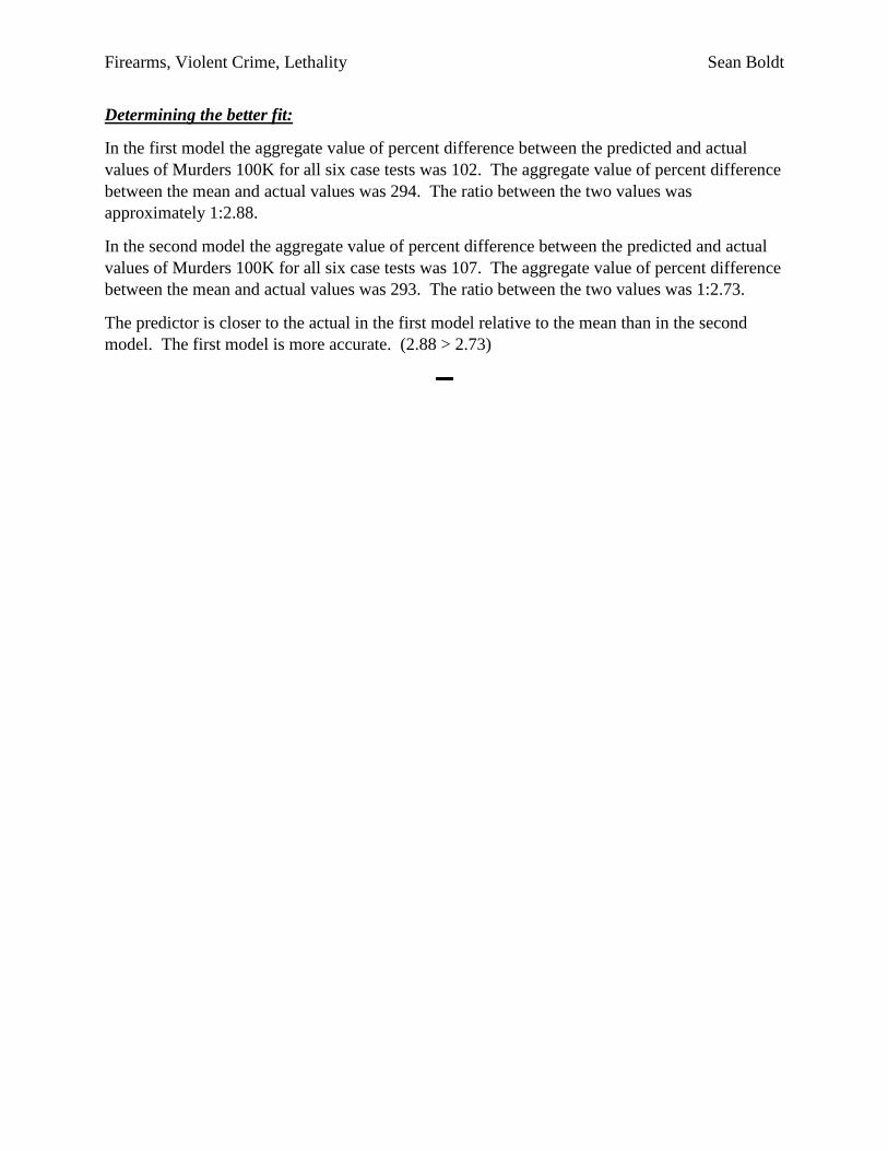
Determining the better fit:
In the first model the aggregate value of percent difference between the predicted and actual
values of Murders 100K for all six case tests was 102. The aggregate value of percent difference
between the mean and actual values was 294. The ratio between the two values was
approximately 1:2.88.
In the second model the aggregate value of percent difference between the predicted and actual
values of Murders 100K for all six case tests was 107. The aggregate value of percent difference
between the mean and actual values was 293. The ratio between the two values was 1:2.73.
The predictor is closer to the actual in the first model relative to the mean than in the second
model. The first model is more accurate. (2.88 > 2.73)
▬