1

Firm Heterogeneity, local externalities and Regional Business

Cycles Differentials

Roberto Basile

Second University of Naples, Faculty of Economics

Corso Gran Priorato di Malta - 81043 - Capua - (CE) roberto.basile@unina2.it

Sergio de Nardis

Nomisma

Strada Maggiore, 44 40125 – Bologna sergio.denardis@nomisma.it

Carmine Pappalardo

National Institute of Statistics (ISTAT)

Piazza dell’Indipendenza, 4 – 00185, Rome (Italy) cpappalardo@istat.it

Abstract. We use microeconomic information to analyze regional differences in business cycle

fluctuations. Working with monthly Italy’s firms data and estimating a random effects ordered

probit model, we first document sizable asymmetries in Northern and Southern firms business

cycles positively related to the intensity of the national cycle. Then, we explore the role of several

firm-specific factors (firm size, export propensity, liquidity constraints, demand conditions,

capacity utilization and expectations) and of local externalities in explaining regional disparities

in business cycle fluctuations. Results suggest that North-South differences in sectoral

composition scantly explain the diverging behaviour of Southern firms, while various firm

specific variables and local externalities capture large part of regional business cycles

differences.

JEL classification: Regional business cycle, firm heterogeneity, local externalities, random

effects ordered probit

Keywords: D21, E32, R10

2

1. Introduction

Regional business cycle analyses traditionally emphasize the role of regional industrial

structure as the major source of divergence in local business cycles. Following the

export-based approach, many studies carried out for the United States and the United

Kingdom argument that the region’s link to the rest of the world is through its export-

base activities so as income fluctuations in the rest of the world are transmitted to the

region through a change in the latter’s export (Domazlicky, 1980). Due to the high inter-

industry heterogeneity in export propensity, regional differences in the industry mix are

therefore the major responsible for regional differentials in business cycle intensity. The

role of industry mix is also highlighted within the “interest rate channel view” of the

monetary policy transmission theory (Carlino and DeFina, 1998; Dedola and Lippi,

2000): the output sensitiveness to a policy induced variation in the short term interest rate

varies significantly across industries, so as the monetary policy may have asymmetric

effects on regions with large differences in the industrial structure. It is puzzling that,

after controlling for industrial composition, these studies find significant regional cyclical

heterogeneity, so as the industry mix can only partially explain these differences.

More recent studies extend the analysis to European economies and question

whether there is an asymmetric regional reaction to monetary policy shocks (Montoya

and de Haan, 2007; Bradley et al., 2004). Some authors also use advanced time series

techniques to analyze co-movements and synchronizations in regional business cycles

and to identify regional specific turning points (see, e.g., Hess and Shin, 1997; Clark and

Shin, 1998; Carvalho and Harvey, 2002; Chen, 2007). With regard to the Italian case,

Mastromarco and Woitek (2007) use annual data for the period 1950-2004 to study the

synchronization of Italian regions’ business cycles. Their results show that regional co-

3

movements vary considerably over time: they were strongest in the 1965–1975 period;

after 1975, regional business cycles started to drift out of phase, with the North leading

the South. The authors argue that North-South business cycle differentials can be

explained with North-South differences in the economic activity (industry mix

explanation) and with North-South differences in political business cycle. Using monthly

data, Brasili and Brasili (2009) also analyze the characteristics and co-movements of

Italian regions’ business cycles to understand the consequences of the global crisis on the

local economies. These authors interpret regional business cycles differentials in terms of

regional product specialisation, regional financial markets development and regional

research intensity.

We claim that all previous studies, focusing on macroeconomic data, disregard the

effect of firm heterogeneity in business cycle behaviour and, thus, they do not clearly

answer the question of why regional business cycles differ. Thus, we suggest to use

microeconomic information in order to distinguish between sector-, and firm-specific

factors in determining regional differences in industrial firms’ business cycle behavior.

To this end, we build up a micro-econometric model so as to assess whether Northern

and Southern firms show significant differences in cyclical behaviour, after having

controlled for structural factors that alter the transmission mechanism of exogenous

shocks.

Working with monthly Italy’s firms data and estimating a random effects ordered

probit model, we first document sizable asymmetries in Northern and Southern firms

business cycles positively related to the intensity of the national cycle: firms located in

the South are more likely to reduce production levels than firms located in the North in

periods of business cycle expansion and viceversa (Section 2). Results also suggest that

North-South differences in sectoral composition scantly explain the lower volatility of

4

Southern firms’ industrial output. Then, we discuss some theoretical hypotheses on the

role of firm specific variables (firm size, export propensity, liquidity constraints,

idiosyncratic demand shocks, capacity utilization and expectations) in business cycle

behaviour and reports the list of microeconomic variables available from business cycle

surveys in Italy (Section 3). According to our assumptions, firm heterogeneity has a role

in explaining regional business cycle differentials only if some spatial contagion is at

work. Empirical evidence corroborates the hypothesis that firm specific variables (mainly

firm size, liquidity conditions and demand conditions) and local externalities capture

large part of regional business cycle differences (Section 4). Section 5 concludes.

2. North-South differences in business cycle: evidence from micro data

2.1 Modelling firms’ business cycle behaviour

To analyse regional differences along the cycle using firm-level information we first

specify an empirical micro-econometric model of firms’ business-cycle behaviour. We

rely on monthly microeconomic data drawn from the business survey carried out by the

Italian National Institute of Statistics (ISTAT). Data are longitudinal and regard 6,629

firms on the period April 2003-December 2010; total number of observations is 308,042.

Qualitative assessment made monthly by each suveyed firm on its level of production is

the dependent variable of the model. We label it as ity for firm 1,...,i N= at time

1,...,t T= ; it takes values 1, 2 and 3 according to firm’s evaluation of production as

‘low’, ‘normal’ and ‘high’, respectively. In addition to their self-reported evaluation of

the production levels, the data set includes many individual characteristics for each

monthly survey, some of which will be used as explanatory variables in our analysis.

5

Given the qualitative nature of the response variable, we use the Ordered Probit

Model with individual random effects (RE-OPM). The basic notion underlying this

model is the existence of a latent continuous variable, *ity , ranging from -∞ to +∞, related

to a set of explanatory variables by the standard linear relationship:

* ' 'it it i it it i i ity x z u x z′ ′= β + γ + = β + γ + ν + ε (1)

where itx is a vector of time-varying regressors, iz is a vector of time-invariant

covariates, β and γ are the associated parameter vectors and it i itu = ν + ε is a random

error term including both time-invariant, iν , and time-varying, itε , unobserved factors.

In model (1) both error components are normally distributed and orthogonal to the set of

predictors. Since the underlying variance of the composite error, 2 2 2u ν εσ = σ + σ , is not

identified, we set 2 1εσ = , so that the residual correlation term is

2 2 2 1 2 2 1, ( ) ( 1)

it isu u− −

ν ν ε ν νρ = σ σ + σ = σ σ + and 1/2[ /(1 )]νσ = ρ − ρ .

Although *ity is unobserved, the integer index ity is observed and related to *

ity by

the following relationship: ity j= (with 1,2,3j = ) iff *1j it jy−µ ≤ ≤ µ where jµ are

unobserved standardized thresholds defining the boundaries between different levels of

ity . In particular, we assume that 0µ = −∞ and Jµ = ∞ . Given the relationship between

ity and *ity , conditional cell probabilities are expressed as:

( )*1

' '1

2 2 2

Pr( | , ) Pr

Pr1 1 1

it it i j it j

j it i j it ii it

v v v

y j x z y

x z x z

−

−

= = µ ≤ ≤ µ

′ ′µ −β − γ µ −β − γν + ε = ≤ ≤ − σ − σ − σ

(2)

Estimations are performed using maximum likelihood. Individual heterogeneity is

unobserved; therefore to obtain the unconditional log-likelihood we need to integrate the

6

conditional log-likelihood. The integration is done with the Gauss-Hermite quadrature

(25 points were chosen) (Greene, 2005). Since the parameters of a latent model do not

have a direct interpretation per se, we refer to marginal probability effects (mpe)

evaluated at the sample average of the predictors. For inference purposes, we also

compute standard errors of mpe using the delta method.

2.2 Capturing national business cycle

We first apply the RE-OPM to monthly firm-level qualitative data to draw estimates of

the quarterly national business cycle. Specifically, we include in the set of regressors

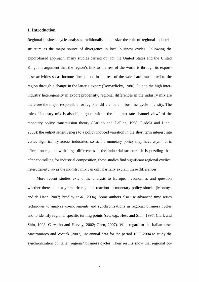
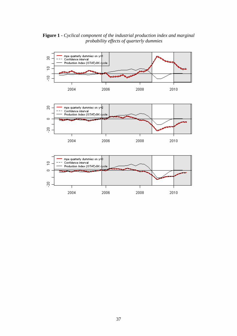
only quarterly dummies. The marginal effects of these dummies on ( )Pr y = 3 (the

probability that the level of production is ‘high’), on ( )Pr y = 2 (‘normal’) and on

( )Pr y = 1 (‘low’) change over time according to business-cycle movements. They are

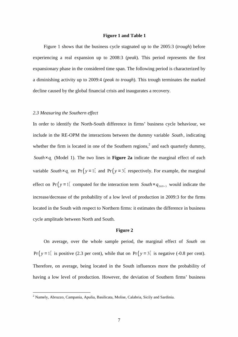
plotted in Figure 1 (continuous red lines) along with the confidence intervals. For

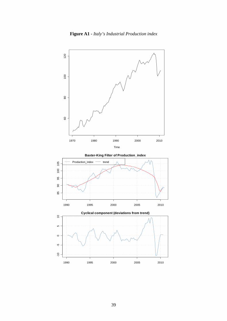
comparison purposes, this figure reports also the cyclical component of the quarterly

index of Italian industrial production (black line) (source: ISTAT) extracted through the

Baxter e King (BK, 1999) filter. This is the so-called deviance business cycle and is used

as benchmark to track business cycle turning points (peaks and troughs) (see also Figure

A1).1 The contemporaneous correlation between the series is rather high (0.67), although

the mpe on ( )Pr y = 3 tend to lead the cyclical component of industrial production as the

correlation peak is at lead 1 (Table 1). Overall, these results encourage us in using the

mpe’s of quarterly dummies as good proxy of the deviance business cycle.

1 It is worthwhile observing that the chronology used here may differ from the one based on the classical

approach to dating the business cycle. The latter considers the levels of the time series to identify the dates

of peaks and troughs that frame economic recession or expansion.

7

Figure 1 and Table 1

Figure 1 shows that the business cycle stagnated up to the 2005:3 (trough) before

experiencing a real expansion up to 2008:3 (peak). This period represents the first

expansionary phase in the considered time span. The following period is characterized by

a diminishing activity up to 2009:4 (peak to trough). This trough terminates the marked

decline caused by the global financial crisis and inaugurates a recovery.

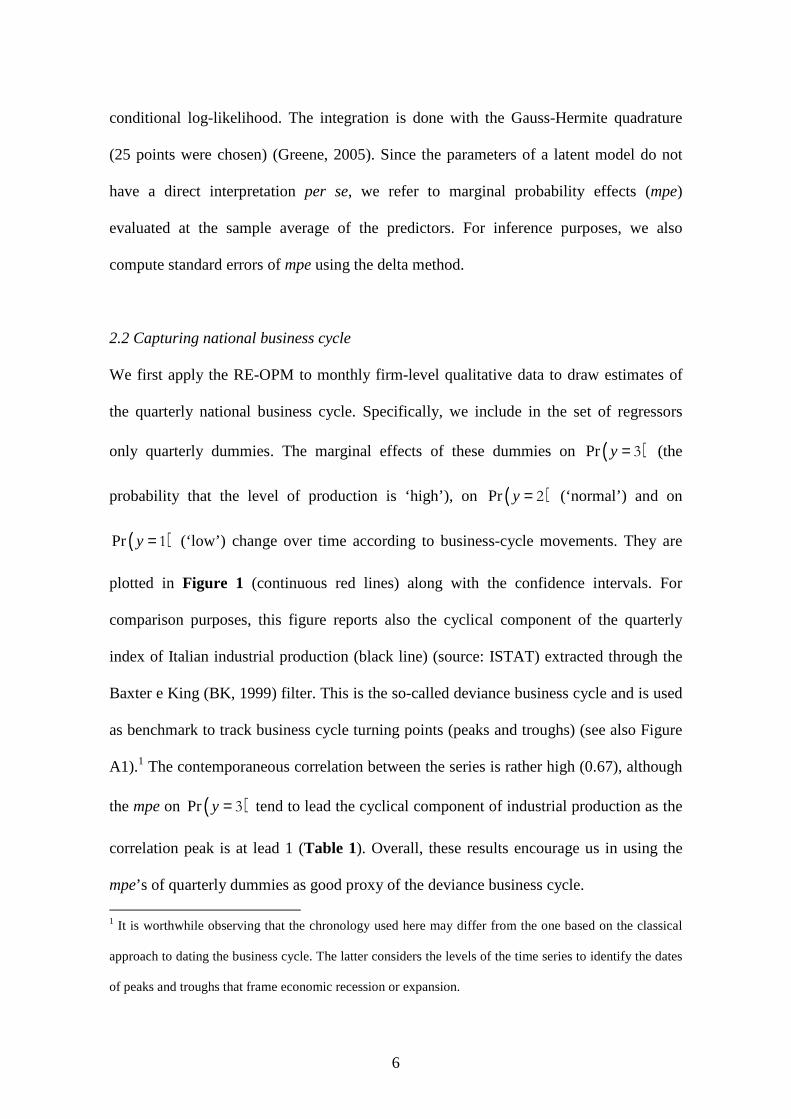
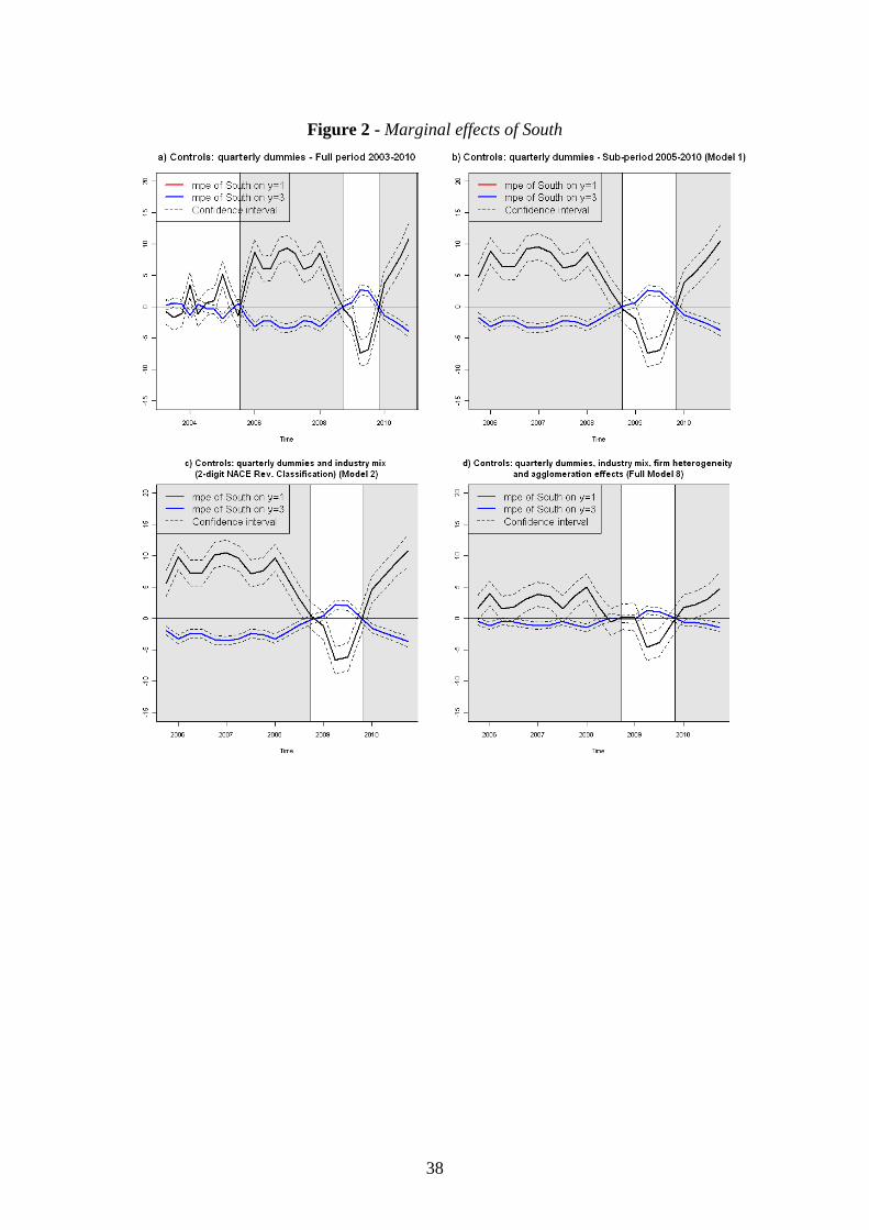
2.3 Measuring the Southern effect

In order to identify the North-South difference in firms’ business cycle behaviour, we

include in the RE-OPM the interactions between the dummy variable South, indicating

whether the firm is located in one of the Southern regions,2 and each quarterly dummy,

tSouth q× (Model 1). The two lines in Figure 2a indicate the marginal effect of each

variable tSouth q× on ( )Pr y = 1 and ( )Pr y = 3 respectively. For example, the marginal

effect on ( )Pr y = 1 computed for the interaction term South q −× 2009 3 would indicate the

increase/decrease of the probability of a low level of production in 2009:3 for the firms

located in the South with respect to Northern firms: it estimates the difference in business

cycle amplitude between North and South.

Figure 2

On average, over the whole sample period, the marginal effect of South on

( )Pr y = 1 is positive (2.3 per cent), while that on ( )Pr y = 3 is negative (-0.8 per cent).

Therefore, on average, being located in the South influences more the probability of

having a low level of production. However, the deviation of Southern firms’ business

2 Namely, Abruzzo, Campania, Apulia, Basilicata, Molise, Calabria, Sicily and Sardinia.

8

cycle behaviour varies greatly during the period, confirming that the degree of regional

“cohesion” along the cycle changes over time (Brasili and Brasili, 2009): standard

deviations of the marginal effect of South on ( )Pr y = 1 and on ( )Pr y = 3 are indeed

much higher than the mean (4.5 and 2.0, respectively). These findings do not change

significantly if estimated over the period 2005:3-2010:4 (Figure 2b), signaling the poor

informative content (in terms of business cycles frequencies) of the initial part of the

sample. Estimates presented below are therefore carried out over the time-span 2005:3-

2010:4, including a well-defined characterization of business-cycle phases.

More specifically, Figures 2a-2b show that the South effect on ( )Pr y = 1 is

negligible (-0.3 percent on average) over the period from 2003:2 to 2005:3, while it is

highly positive (6.9 percent on average, see Table 2 first row) in the expansion period

2005:4-2008:3, indicating a difficulty of Southern firms to participate to the recovery.

During the recession period (2008:4-2009:4), the marginal effect of South on ( )Pr y = 1

becomes strongly negative (-3.7 percent on average), indicating a lower penalization of

Southern firms with respect to Northern ones. Finally, in the upturn started on 2010:1 the

South effect on ( )Pr y = 1 is again highly positive (7 percent on average), confirming the

lower capacity of Southern firms to join the positive cycle.

Table 2

It is worth noticing that if regional business cycles were not synchronized, a

significant marginal effect of South could not be correctly interpreted as evidence of

regional difference in business cycle amplitude. However this is not the case: evidence

on the high degree of regional cyclical co-movements is provided in terms of cross-

correlations between the relative frequencies of firms’ assessment on production levels to

be low (y=1), normal (y=2) or high (y=3) in the North and in the South (Table 3).

9

Table 3

2.4 The role of industry mix

In this section we discuss the results of an analysis aimed to test whether North-South

differences over the cycle depend on heterogeneous specialization of the two regions.

Among the regressors of the model we include sector dummies (using the 2-digit NACE

Rev. 1 classification), besides the quarterly dummies and the interaction variables

tSouth q× (Model 2).3 Table 4 shows the contribution of sector heterogeneity in

explaining firms’ business cycle behavior: the log-likelihood moderately increases with

respect to Model 1 (including only quarterly dummies and tSouth q× ); the AIC slightly

decreases, while the BIC does not change and the goodness of fit does not considerably

improve.

Table 4

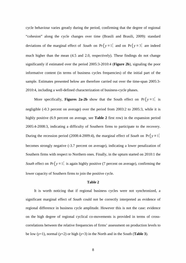
Figure 2c displays the marginal effects of tSouth q× while Table 2 reports their

mean values and test for their statistical difference against Model 1. The effect of South

on ( )Pr y = 1 is again highly positive for both expansion periods (2005:4-2008:3 and

2010:1-2010:4) and highly negative in the recession period (2008:4-2009:4). However,

with respect to Model 1, the marginal effects of South on ( )Pr y = 1 in expansion periods

increase contrary to the assumption of the industry mix view (see t-tests in parenthesis in

Table 2). This means that if North and South had the same industrial structure, the

regional difference in business cycle amplitude would be higher. A slight improvement

3 All manufacturing sectors, defined according to the international standard classification NACE_rev1

(Subsections 15-36), are included.

10

against Model 1 is observed for the marginal effects of tSouth q× on ( )Pr y = 3 (1

against 1.3) and on ( )Pr y = 1 (-2.9 against -3.7) during recession, although this

difference is not significantly different from zero. Similar findings are obtained using

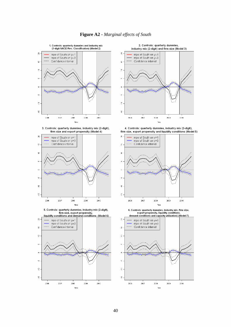
more detailed sector specification (3 digit level) (Figure A2.1). This evidence suggests

that the industry mix does not help explain regional differences in business cycle. More

inspection is therefore needed taking stocks of the rich firm-level information

characterizing the dataset.

3. Working hypotheses

In 1966 Siegel posed a relevant issue: “The really interesting question … is whether or

not regions differ from each other in cyclical performance for reasons other than industry

mix” (Siegel, 1966, p. 44). Results discussed so far show that this is still an open issue

and an effort is required to explain regional business-cycle differences in terms of

entrepreneurial composition (firm heterogeneity). Various strands of literature act as

guide for selecting the firm-specific variables able to affect, in our model, the ordinal

indicator for the level of production. In what follows, we describe them, with brief

discussion of theoretical underpinnings.

3.1 Borrowing constraints (firm size)

The role of microeconomic heterogeneity along the cycle has been firstly emphasized in

theories of monetary transmission. Specifically, firm size may be responsible for the

transmission of monetary shocks through the so called “balance-sheet” and the “bank-

lending” channels (Bernanke and Gertler, 1995; Carlino and DeFina, 1998; Guiso et al,

2000; Ehrmann, 2000; Dedola and Lippi, 2000). In the balance-sheet view, given

11

asymmetric information, access to credit depends on the value of firms’ assets, acting as

collateral. A monetary tightening can reduce the latter by deteriorating balance sheets.

Firms of different size are differently exposed to credit squeeze: given lower value of

assets and higher amount of required collateral, small firms are likely to be more credit

constrained than large ones.

Size matters in monetary transmission also for the bank-lending view. A tighter

monetary policy reduces the amount of credit for borrowers when the central bank has a

leverage over the volume of intermediated credit. Small firms, more dependent on

intermediated credit, are adversely affected; large firms can instead rely on easier access

to other forms of external finance (Christiano et al., 1996; Ehrmann, 2000; Dedola and

Lippi, 2000).4 Moreover, Carlino and DeFina (1998) have found evidence for the US that

asymmetric spatial distribution of small firms is partially responsible for different output

effects of monetary policy shocks across regions. This is relevant for our investigation as

it is possible to hypothesize that North-South differences in firm size composition are

partly responsible for North-South business cycle differentials (H.1).

4 The analyses of the effect of firm size on the transmission of monetary policy shock quoted above are

based on the use of Structural VAR approaches. They first identify either sectoral or regional differences in

the output effect of unanticipated monetary policy shocks by means of impulse response functions and then

use aggregated size composition measures (either at sectoral or regional level) as determinants of the

monetary policy impacts. The spirit of our analysis is partially different from these studies since we are

essentially interested in assessing the existence of regional disparities in business cycle fluctuations after

controlling for most of the firm level factors affecting the mechanism of real and monetary shocks

transmission. Moreover, we want to exploit all firm heterogeneity, avoiding to use aggregated size

composition measures.

12

We use the logarithm of the number of employees (ln emp) as proxy for capital

market access (ability to borrow), so as we expect a positive effect of firm size on the

probability to produce a high level of output, ( )Pr y = 3 , and a negative effect on the

probability to produce a low level of output, ( )Pr y = 1 . Uncertainty remains as for the

probability to produce a normal level of output, ( )Pr y = 2 . We might also expect time

heterogeneity in the influence of firm size, as suggested by the studies quoted above.

Thus, we include in our model interactions between firm size and temporal dummy

variables indicating whether the economy is in boom or recession. We also control for

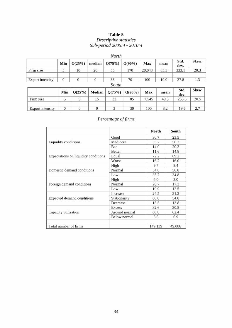
possible nonlinearities by introducing the square term of lnemp. Table 5 reports

descriptive statistics of the firm-level variables included in our models: on average

Southern firms are smaller than Northern ones.

Table 5

3.2 Liquidity constraints

Liquidity constraints are a further possible cause of firm heterogeneity over the cycle.

With borrowing limitations, entrepreneurs must finance their investments partly from

selling their holdings of money and equity. In this case, different liquidity degrees of

equities may affect differently entrepreneurs' investment (Kiyotaki and Moore, 2008).5

It is reasonable to assume that the effect of firms’ liquidity constraints on the real

economy are not randomly diffused over space, at least for two reasons: first, firms

5 An example of a liquidity shock which reduces re-saleability of equity persistently is represented by the

recent financial turmoil that made assets that used to be liquid scantly re-saleable. Naes et. al. (2010) also

document that, in the US case, measures of stock market liquidity contain leading information on the real

economy at least since 2nd World War.

13

located nearby have relatively denser vertical input-output linkages than those located

further apart, so as an adverse liquidity shock on an entrepreneur propagate to short-run

output of other firms with a distance decay effect; second, adverse liquidity conditions

may have a regional dimension to the extent they are induced by specific difficulties of

the local banking sector. On the grounds of these considerations one may hypothesize

firms' liquidity conditions as possible source of regional business cycle differentiation

(H.2).

Liquiditity conditions are captured by two dummy variables indicating whether the

firm considers its liquidity as good, mediocre or bad (reference category). We expect a

positive (negative) effect of good liquidity conditions on ( )Pr y = 3 ( ( )Pr y = 1 ). Table 5

shows that the percentage of firms with good liquidity conditions is higher in the North

than in the South.

Since firms’ production decisions are forward looking, it is important to take

expectations into account in our analysis. Business opinion surveys collect considerable

information on firms’ expectations about liquiditiy conditions. We exploit this

information by introducing dummy variables indicating, respectively, whether the firm

expects for the next period better, equal or worse (reference cateogory) liquidity

conditions.

3.3 Export propensity

Even in the export-based view it is not reasonable to assume that regional differences in

industry mix properly capture regional differences in export propensity. This is because,

as shown by a broad literature (e.g., Basile, 2001; Bernard and Jensen, 2004; Melitz and

14

Ottaviano, 2008), also within homogeneous industries there is huge firm heterogeneity in

export propensity.

Obviously, if exporters were randomly distributed over space, intra-industry firm

heterogeneity in export propensity would not help explain regional differentials in the

diffusion of international business cycle. Yet, there is evidence of asymmetric spatial

distributions of exporters reflecting substantial local spillovers: individual decisions to

export are influenced by the presence of nearby exporters (Koenig et al., 2010).

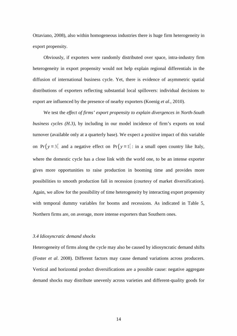
We test the effect of firms’ export propensity to explain divergences in North-South

business cycles (H.3), by including in our model incidence of firm’s exports on total

turnover (available only at a quarterly base). We expect a positive impact of this variable

on ( )Pr y = 3 and a negative effect on ( )Pr y = 1 : in a small open country like Italy,

where the domestic cycle has a close link with the world one, to be an intense exporter

gives more opportunities to raise production in booming time and provides more

possibilities to smooth production fall in recession (courtesy of market diversification).

Again, we allow for the possibility of time heterogeneity by interacting export propensity

with temporal dummy variables for booms and recessions. As indicated in Table 5,

Northern firms are, on average, more intense exporters than Southern ones.

3.4 Idiosyncratic demand shocks

Heterogeneity of firms along the cycle may also be caused by idiosyncratic demand shifts

(Foster et al. 2008). Different factors may cause demand variations across producers.

Vertical and horizontal product diversifications are a possible cause: negative aggregate

demand shocks may distribute unevenly across varieties and different-quality goods for

15

the mere fact that consumers with different tastes experiment heterogeneous demand

variations.

Firm-level idiosyncratic demand shifts may induce regional differences in the

business cycle if agglomeration is at work. The latter favours spatial concentration of

firms producing similar varieties (e.g. industrial districts) or of firms that are tied by

vertical input-output links. Moreover, within spatial clusters of small firms it is more

likely the formation of persistent customer-supplier relationships. In all these cases a

variety-specific demand shock may end up by diffusing to a whole territory with a

distance decay effect.

These considerations lead us to introduce in empirical testing firm-level demand

conditions as a further potential source of regional differentiation of business cycle

(H.4). Specifically, we control for the cyclical demand conditions at home and abroad,

proxing them by domestic and foreign orders. Firms are asked to indicate whether the

domestic and foreign demand level is high, normal or low over the reference period.

Thus, we introduce four dummy variables (low levels are used as reference categories)

and expect a positive effect of these dummies on the dependent variable. We also exploit

information on demand expectations and introduce dummy variables indicating,

respectively, whether the firm expects for the next period an increase, a stationarity or a

decrease (reference cateogory) of its demand level. Table 5 signals that the percentage of

firms with high demand conditions is, on average, higher in the North than in the South.

3.5 Capacity utilization

The issue of firm heterogeneity is also remarked in recent contributions to the real

business cycle literature analyzing the role of idle productive capacities in propagating

technological shocks (Fagnart et al., 1999). Given limited input substitution in the short

16

run, uncertainty at the time of capacity choices can explain why the installed productive

equipments of the economy are usually underutilized in equilibrium. Moreover,

idiosyncratic demand uncertainty can explain why some firms produce at full capacity

while others face excess capacities. In these models, the proportion of firms with excess

capacity plays an important role in magnifying and propagating aggregate technological

shocks.

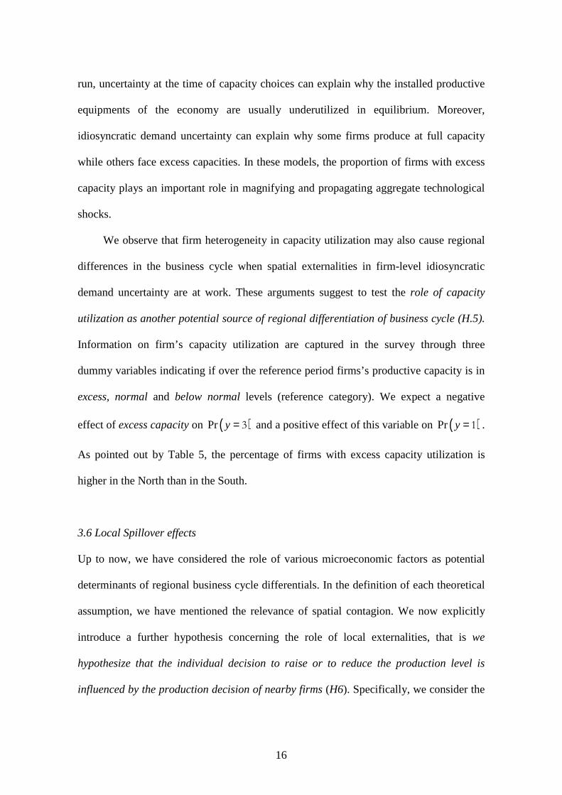
We observe that firm heterogeneity in capacity utilization may also cause regional

differences in the business cycle when spatial externalities in firm-level idiosyncratic

demand uncertainty are at work. These arguments suggest to test the role of capacity

utilization as another potential source of regional differentiation of business cycle (H.5).

Information on firm’s capacity utilization are captured in the survey through three

dummy variables indicating if over the reference period firms’s productive capacity is in

excess, normal and below normal levels (reference category). We expect a negative

effect of excess capacity on ( )Pr y = 3 and a positive effect of this variable on ( )Pr y = 1 .

As pointed out by Table 5, the percentage of firms with excess capacity utilization is

higher in the North than in the South.

3.6 Local Spillover effects

Up to now, we have considered the role of various microeconomic factors as potential

determinants of regional business cycle differentials. In the definition of each theoretical

assumption, we have mentioned the relevance of spatial contagion. We now explicitly

introduce a further hypothesis concerning the role of local externalities, that is we

hypothesize that the individual decision to raise or to reduce the production level is

influenced by the production decision of nearby firms (H6). Specifically, we consider the

17

possibility of local externalities at a fine geographical level corresponding to the province

(103 in Italy).

Production externalities are not only very likely to be localized, but they are also

very likely to depend on the degree of agglomeration of firms in the same area that is by

the density of economic activity within the province. The agglomeration of firms in the

same area may give rise to both market externalities (input-output linkages) and non-

market (technological) externalities, but also to higher competition. An example of

market externalities is the cost-sharing devices that allow firms to communicate together

on their products to final consumers. Non-market externalities involve informal

information transfers, which may benefit local firms through a decrease in variable or

fixed costs. We therefore measure local externalities by multiplying the employment

density in the province where firm i is located and the balance of the production level in

the same province, i.e. the difference between the percentage of firms (excluding firm i)

which evaluate the production level as ‘high’ and the percentage of firms (excluding firm

i) which evaluate the production level as ‘low’.

Combining H.1-H.6, we can say that regional differences in the entrepreneurial

mix (in terms of size, liquidity conditions, export intensity, demand shifts, capacity

utilization and expectations) may contribute to explain regional differences in business

cycles along with the industry mix and local externalities.

4. Evaluating the effects of firm heterogeneity in explaining North-South

business cycle differentials

4.1 Econometric issues

18

In section 2.4 we have discussed the role of sectoral composition in capturing North-

South business cycle differentials. The model was specified by including sectoral and

time dummies and the interactions between the dummy South and time dummies. We

now progressively extend that model by including the firm level variables listed above.

The aim is to verify whether controlling for the firm-specific variables leads to an

abatement of regional disparities in business cycle fluctuations. Before presenting the

results of this analysis, however, some methodological issue have to be discussed.

In describing the RE-OPM in section 2.1 we have assumed orthogonality between

error components and the set of predictors. However, if the explanatory variables and the

individual specific effects are correlated, the RE-OPM may lead to inconsistent

estimates. According to Wooldridge (2002), a possible route to overcome this issue

consists of including time averages of the time-varying variables ( ix ) as additional time-

invariant regressors. Modelling the expected value of the firm-specific error as a linear

combination of the elements of ix - ( | , )i it i iE x z x′ν = ψ - so that i i ix′ν = ψ + ξ , we may

recast model (1) as:

* ' ( ) ( )it it i i i i ity x x x z′ ′= β − + ψ + β + γ + ξ + ε (3)

where ψ is a conformable parameter vector and iξ is an orthogonal error with respect to

ixψ′ . Also, we assume both errors iξ and itε to be normally distributed conditionally on

itx ’s and iz ’s. In (3), the deviations from the averages per individual capture shock

effects (within-effect), while the means identify level effects (between effects). Including

within and between effects aims at introducing dynamics in the model, because the mean

value changes gradually when months pass by (Van Praag et al., 2003).

A further issue is a possible endogeneity problem affecting equation (3). While the

information provided by the survey possess the desirable property of being internally

19

consistent (it is the “same” individual firm providing all the requested information on its

activity), it is likely to expect that the variables involved may be “intrinsically”

endogenous. For example, an entrepreneur anticipating positive (or negative) demand

shocks on either domestic or foreign markets could hire (or lay off) employees to adapt

its supply capacity to demand. We thus face a reverse causality and a simultaneity issue

relative to firm characteristics variables. Moreover, higher production levels raise ex-post

employment growth rates. Direction of causality between firms' size and their production

behavior is consequently not clearly determined. Parallel issues can be raised on the

spillover variable. If firm i 's production behavior depends on the surrounding firms'

behavior, the latter is itself impacted by firrm i 's production performance, which induces

a reverse causality problem. Further, simultaneity may be an issue, since unobserved

supply-side or demand-side shocks could affect both the production performance of firm

i and the performance of its neighbors. To control for the potential circularity and

simultaneity problems, we lag all right-hand side variables one period.

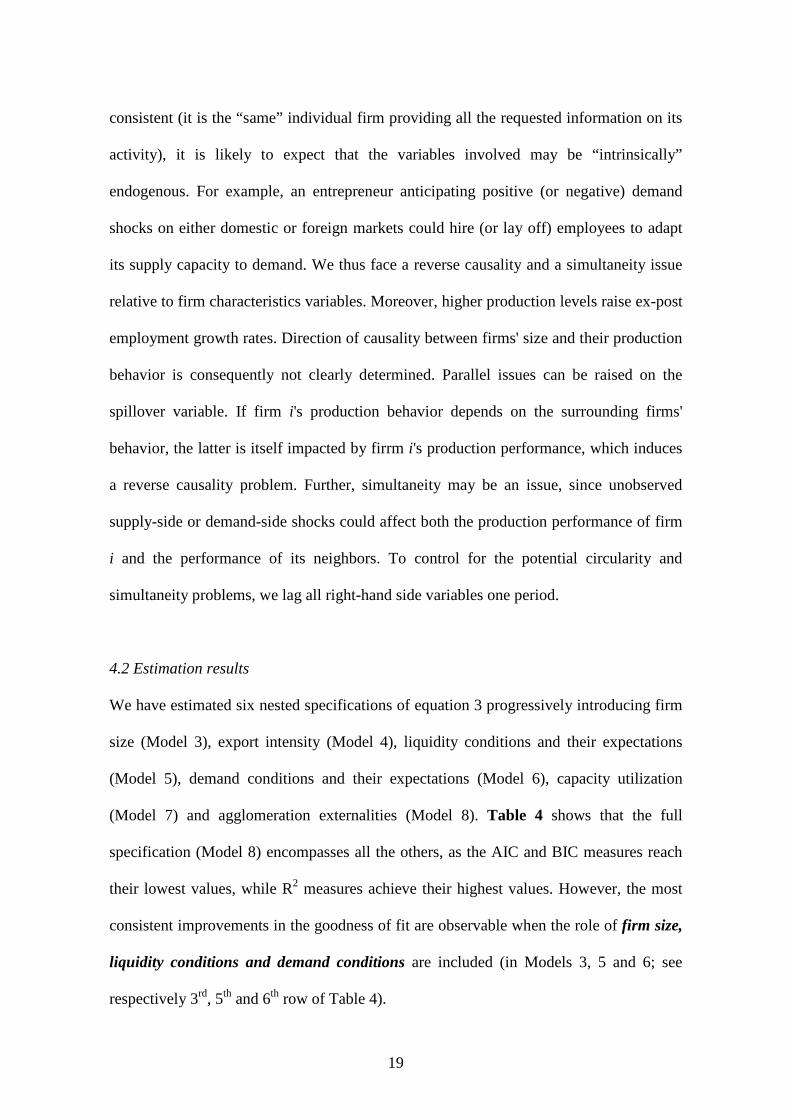
4.2 Estimation results

We have estimated six nested specifications of equation 3 progressively introducing firm

size (Model 3), export intensity (Model 4), liquidity conditions and their expectations

(Model 5), demand conditions and their expectations (Model 6), capacity utilization

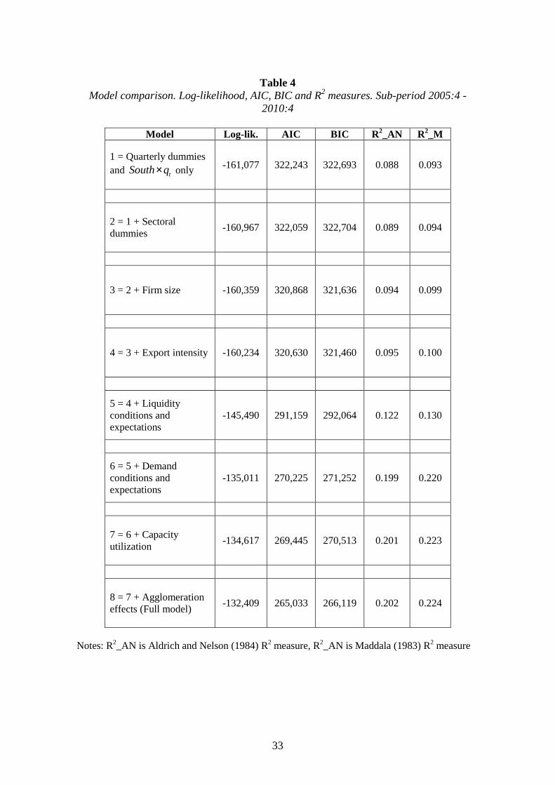
(Model 7) and agglomeration externalities (Model 8). Table 4 shows that the full

specification (Model 8) encompasses all the others, as the AIC and BIC measures reach

their lowest values, while R2 measures achieve their highest values. However, the most

consistent improvements in the goodness of fit are observable when the role of firm size,

liquidity conditions and demand conditions are included (in Models 3, 5 and 6; see

respectively 3rd, 5th and 6th row of Table 4).

20

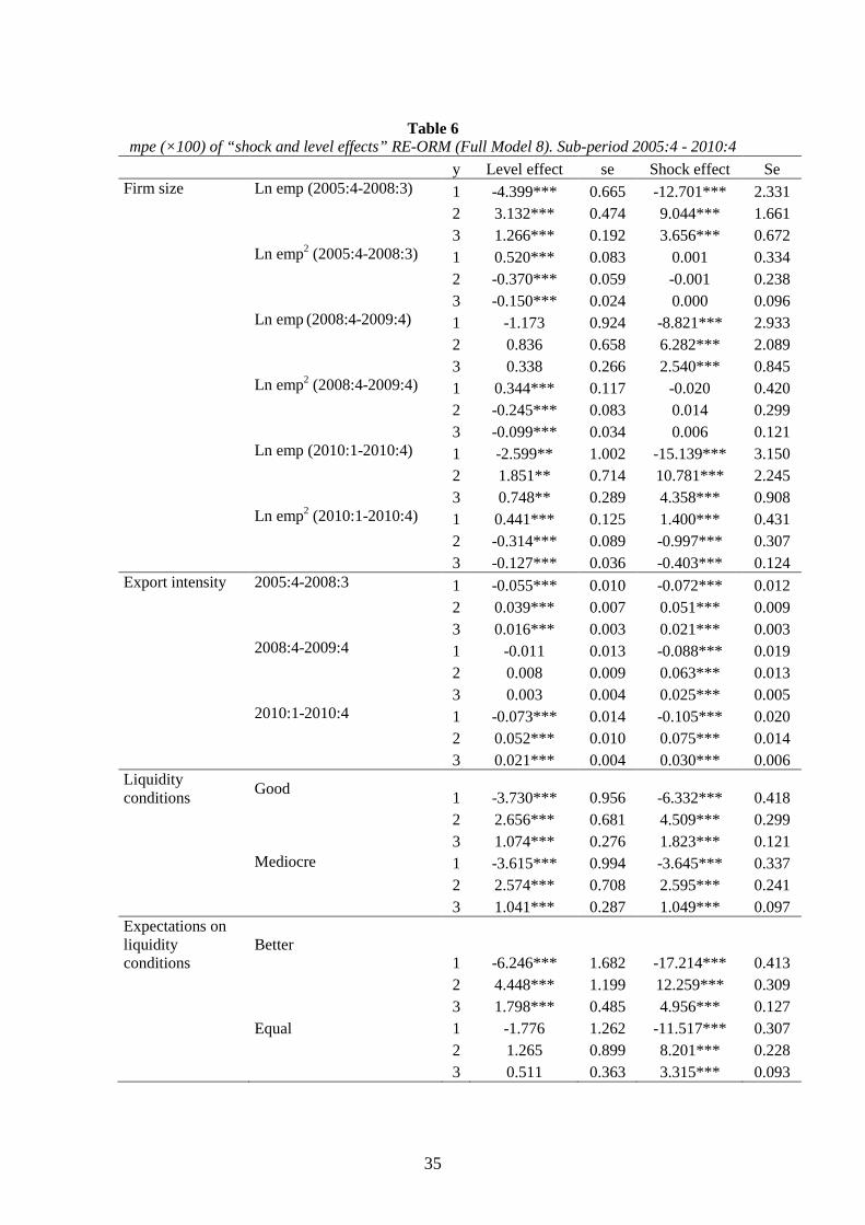
Table 6 reports marginal probability effects (mpe) of the firm-specific variables

for the full Model (8).6 As mentioned above, we have estimated both the “Shock effect”

and the “Level effect”: the first refers to mpe of the deviations from the individual

average, while the mpe for the “Level effect” denote the differences between individuals

(a sort of between effect). In the discussion of the results we focus on the “Shock

effects”, as they mimic the within firm effects obtained from a fixed effects estimation.7

Table 6

Firm size has a positive and significant effect in all three sub-periods, while its

squared term is significant and enters negatively, depicting an inverted U-shaped

relationship, only in the third period. The mpe indicate that for an increase of 1% in firm

size, the predicted probability of having a low level of production, Pr( 1)ity = , lowers by

13-15% in the expansion periods, while it decreases by 8% in the recession period.

Conversely, the probability of having a high level of production, Pr( 3)ity = , increases by

4% in the expansion periods and by 2.5% in the recession period. We can therefore

conclude that the effect of firm size is higher in the expansion periods rather than in

recession. Moreover, firm size affects more the probability that the level of production is

low, rather the probability that is normal or high. Considering that interest rates move in

the upside during a boom (and downside in a recession), these results are in line with the

theoretical underpinnings depicted above.8

6 The results of the other intermediate models are available upon request.

7 The fixed thresholds, 1µ and 2µ , are statistically significant at the 1 percent level and different from 1,

pointing out that the three ordinal categories are not equally spaced, refraining us to use OLS techniques.

8 Imagine, for example, an intervention of the Central Bank that raises the interest rate during an expansion

period. According to both the balance-sheet and bank-lending views, the monetary policy shock is likely to

21

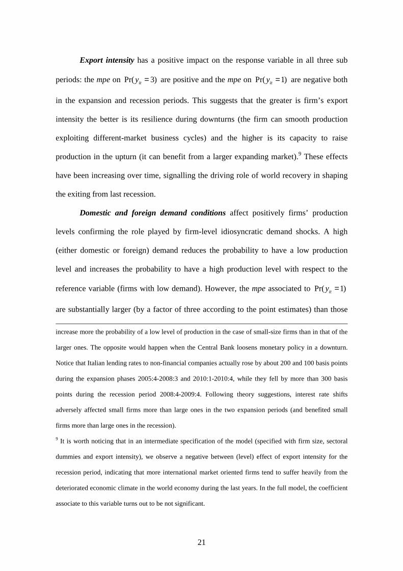
Export intensity has a positive impact on the response variable in all three sub

periods: the mpe on Pr( 3)ity = are positive and the mpe on Pr( 1)ity = are negative both

in the expansion and recession periods. This suggests that the greater is firm’s export

intensity the better is its resilience during downturns (the firm can smooth production

exploiting different-market business cycles) and the higher is its capacity to raise

production in the upturn (it can benefit from a larger expanding market).9 These effects

have been increasing over time, signalling the driving role of world recovery in shaping

the exiting from last recession.

Domestic and foreign demand conditions affect positively firms’ production

levels confirming the role played by firm-level idiosyncratic demand shocks. A high

(either domestic or foreign) demand reduces the probability to have a low production

level and increases the probability to have a high production level with respect to the

reference variable (firms with low demand). However, the mpe associated to Pr( 1)ity =

are substantially larger (by a factor of three according to the point estimates) than those

increase more the probability of a low level of production in the case of small-size firms than in that of the

larger ones. The opposite would happen when the Central Bank loosens monetary policy in a downturn.

Notice that Italian lending rates to non-financial companies actually rose by about 200 and 100 basis points

during the expansion phases 2005:4-2008:3 and 2010:1-2010:4, while they fell by more than 300 basis

points during the recession period 2008:4-2009:4. Following theory suggestions, interest rate shifts

adversely affected small firms more than large ones in the two expansion periods (and benefited small

firms more than large ones in the recession).

9 It is worth noticing that in an intermediate specification of the model (specified with firm size, sectoral

dummies and export intensity), we observe a negative between (level) effect of export intensity for the

recession period, indicating that more international market oriented firms tend to suffer heavily from the

deteriorated economic climate in the world economy during the last years. In the full model, the coefficient

associate to this variable turns out to be not significant.

22

related to Pr( 3)ity = suggesting that firm-specific demand shocks differentiate the

business-cycle behaviour between high- and low-demand firms mainly through the

modality of ‘low production’. Notice that firm-specific demand captures idiosyncratic

shocks: this means that even for firms of the same sector, facing the same aggregate

demand, there are more or less opportunities to change production, with respect to other

producers, according to the variety they produce, the market where they sell and,

possibly, the long-run relationship the have with their clients. Estimation results also

point out that production levels are affected by expectations on future demand in a

similar, although less intense, way as for current demand.

Liquidity conditions turn out to be statistically significant in explaining output

dynamics for Italian manufacturing firms. In line with expectations, the mpe’s of good

liquidity conditions on Pr( 1)ity = is negative and the one on Pr( 3)ity = is positive.

Again the negative probability effect on the ‘low production’ is larger (in absolute terms)

than the positive marginal effect on ‘high production’, signalling also for this effect that

the ‘low production’ modality is the one that mainly discriminates firm-by-firm cyclical

behaviour. Interestingly, expectations on future liquidity conditions seem to play a more

relevant role than assessment on current conditions. Considering liquidity constraints on

entrepreneurs’ investment as a source of firm-level differentiation of the business cycle,

these findings would indicate that it is the evaluation of liquidity on a long time span that

affects current investment decisions and production levels.

Capacity utilization has proved to play a significant role in detecting individual

production behaviour over the business cycle. As predicted on the ground of theory,

excess capacity has a positive mpe on Pr( 1)ity = and a negative mpe on Pr( 3)ity = , with

the former effect (also in this case) being larger than the latter: firms with underutilized

23

capacity are more likely to reduce production (and less likely to increase it) than firms

with a normal rate of capacity utilization.

Finally, our results corroborates the hypothesis that agglomeration externalities

affect short term firms’ output decisions. Our measure of local externalities has indeed a

positive and significant effect on Pr( 1)ity = and a negative mpe on Pr( 3)ity = : firms

located in provinces with higher employment density and diffused high production levels

are more likely to increase production (and less likely to reduce it).

4.3 Firm heterogeneity and the North-South divide

To check whether the consideration of firm-specific variables reduces the North-South

difference in business-cycle amplitude, we have to control for changes in the dimension

of the marginal effects of tSouth q× following the inclusion of such variables in the

model. Figure 2d shows the marginal effects of tSouth q× after having controlled for

sectoral mix, firm heterogeneity and local externalities (Model 8). Comparing Figure 2d

(Model 8) with Figures 2b (Model 1, where there are no other controls than quarterly

dummies) and with Figures 3c (Model 2, where the only control for industry mix is

added), it appears quite clear that North-South differences in firm composition (in terms

of size and export propensity) and firm behavior (in terms of demand, liquidity

conditions and capacity utilization) as well as in local externalities are mostly responsible

for the deviation of Southern firms’ from the cyclical behavior of Northern firms. Indeed,

with Model 8 confidence intervals of the marginal effects contain the horizontal zero line

10 out 21 times.

From Table 2 we also learn that the probability of a low level of production,

( )Pr y = 1 , is still higher when the firm is located in the South during the expansion

24

period 2005:4-2008:3 (2.6 per cent, see last row of Table 2) and in the recent period of

slow recovery (3 per cent). However, these percentages are much lower than those

computed with Model 1 (6.9 and 7.0 per cent, respectively) and Model 2 (7.9 and 7.8 per

cent, respectively), indicating that firm heterogeneity is responsible for more than 60 per

cent of the deviation of Southern firms’ from the cyclical behavior of Northern firms

during the periods of boom. This value raises up 70 per cent when considering the

probability of high level of production, ( )Pr y = 3 . When we consider instead the

recession period 2008:4-2009:4, the negative effect of South on ( )Pr y = 1 with model 8

(-1.8 per cent) is 50 percent lower than in Model 1, but only 37 percent lower than in

Model 2, suggesting that sector composition has been responsible along with firm

heterogeneity and local externalities in explaining the North-South divide during the

downswing period. Moreover, the difference between the average marginal effects of

South computed with Model 8 and those computed with Model 1 (used as the

benchmark) turns out to be statistically significant in all sub-periods (see t-tests in square

brackets in Table 2).

Going from Model 2 to 8, it is possible to learn from Table 2 and Figure A2 that

during the expansion periods (2004:4-2008:3 and 2010:1-2010:4) the most influent firm-

level variables in affecting the marginal effect of tSouth q× are firm size, liquidity

conditions and demand conditions. Specifically, testing more formally the statistical

difference between the marginal effects of tSouth q× computed with the eigth different

nested models, it comes out that this group of variables is able to capture North-South

differences during the expansion periods (see t-tests in parenthesis in Table 2). In

recession, the regional difference in business cycle amplitude can only be explained by

the joint effects of all the variables (see t-tests in square brackets in Table 2).

25

All in all, these findings suggest that microeconomic characteristics of Italian

firms have considerable predictive power regarding North-South differences in cyclical

fluctuations. However, these firm-level characteristics together with consideration of

sector composition and local externalities do not help explain the entire observed

amplitude divide, in particular over the two expansion periods identified in considered

time span. In other words, despite the control for local externalities, firms with similar

individual characteristics and belonging to the same industrial sector, but located in

different regions, continue to show a different business cycle behaviour. This tells that

the regional institutional environment (for example, a difference in regional financial

institutions) is still important to explain regional business cycle differences.

5. Conclusions

This study represents a first attempt to empirically analyze the role of firm heterogeneity

in regional business cycle behaviour. Previous studies based on macroeconomic data

have tried to explain business cycle differentials across regions in terms of differences in

the sectoral mix, disregarding the potential role of different firm level variables that

various strands of business cycle theory have identified as mechanisms of transmission of

real and monetary shocks (firm size, liquidity constraints, export orientation, firm

specific demand conditions, capacity utilization and expectations).

Using business survey monthly data for a sample of Italy’s manufacturing firms

spanning the years from 2003 to 2010, we try to assess whether Southern firms’ business

cycle behaviour is different in amplitude from that of the rest of the country. The results

obtained can be read subdividing the time span in four periods: the first one (from the

second quarter of 2003 until the third quarter of 2005) is characterized by a stagnation of

26

economic activity; the second one (from the fourth quarter of 2005 until the third quarter

of 2008) is a period of boom; the third period (from the fourth quarter of 2008 to the

fourth of 2009) is characterized by an economic recession; in the last period there are

signs of recovery. Our results suggest that Southern firms are more likely to reduce

production levels more than firms located in North in periods of business cycle expansion

and viceversa. Finally, we assess whether, after controlling for several firm- and sectoral

specific factors as well as for local externalities, there are still regional disparities in

business cycle fluctuations. Results suggest that regional differences in the sectoral

composition partly explain the diverging behaviour of Southern firms during the

recession period, while various firm specific variables (specifically firm size, demand

conditions and liquidity conditions) capture large part of regional business cycles

differences both during periods of recession and boom.

The main contribution of the paper is three-fold. First, it offers a method to

identify regional business cycle differentials (in terms of cyclical amplitude) in the

absence of official regional statistical information. Secondly, this study represents a first

attempt to empirically analyze the role of firm heterogeneity in regional business cycle

behaviour based on micro-data. It allows to properly estimate the effect of different

factors suggested by the theory. Finally, the relevance of the study stands also on its

replicability in other European countries that collect the same kind of business cycle

information through the European Commission harmonised questionnaire. The method

proposed in the paper can also be extended to analyse inter-sectoral or even inter-country

differentials in business cycle behaviour.

References

27

Basile R. (2001), Export Behaviour of Italian Manufacturing Firms Over the Nineties:

the Role of Innovation. Research Policy, 30, 1185-1201

Baxter M. and King R.G. (1999), Measuring business cycles: Approximate band pass

filters. The Review of Economics and Statistics, 81, 575–593.

Bernanke B.S. and Gertler M. (1995), Inside the Black Box: The Credit Channel of

Monetary Policy Transmission. Journal of Economic Perspectives, 9, 27-48

Bernard A. B. and Jensen J. B. (2004), Why Some Firms Export. Review of Economics

and Statistics, 86, 561-569

Bradley J., Morgenroth E. and Untiedt G. (2004), Macro-regional evaluation of the

Structural Funds using the HERMIN modelling framework. Mimeo

Brasili A. and Brasili C. (2009), Sincronia e distanza nel ciclo economico delle regioni

italiane. Politica Economica, 2, Il Mulino, Bologna

Carlino G. and DeFina R. (1998), The Differential Regional Effects of Monetary Policy.

Review of Economics and Statistics, 80, 572-587

Carvalho V.M. and Harvey A. C. (2002), Growth, Cycles and convergence in US

regional time series. Mimeo

Chen S.W. (2007), Using Regional Cycles to Measure National Business Cycles in the

U.S. with the Markov Switching Panel Model. Economics Bulletin, 3, 1-12

Christiano L., Eichenbaum M., Evans C. (1996), The effects of monetary policy shocks:

evidence from the flow of funds. Review of Economics and Statistics, 78, 16–34

Clark T.E. and Shin K. (1998), The sources of fluctuations within and across countries.

Research Working Paper Federal Reserve Bank of Kansas City, 98-04

28

Dedola L. and Lippi F. (2000), The Monetary Transmission Mechanism: Evidence from

the Industries of Five OECD Countries. Papers 389, Banca d’Italia - Servizio di Studi

Domazlicky B. (1980), Regional Business Cycles: A Survey. Regional Science

Perspectives, 10, 15-34

Ehrmann M. (2000), Firm size and monetary policy transmission: evidence from German

business survey data. Working Paper Series 21, European Central Bank

Fagnart J.O., Licandro and F. Portier (1999), Firm Heterogeneity, Capacity Utilization

and the Business Cycle. Review of Economic Dynamics, 2, 433-455

Foster L., Haltiwanger J. And Syverson C (2008), Reallocation, Firm Turnover, and

Efficiency: Selection on Productivity or Profitability? American Economic Review,

98, 394-425

Greene W. H. (2005), Econometric Analysis. New Jersey: Prentice-Hall.

Guiso L., Kashyap A.K., Panetta F. and Terlizzese D. (1999), Will a Common European

Monetary Policy have Asymmetric Effects? Economics Perspectives, Federal

Reserve Bank of Chicago, 56–75

Hess G.D. and Shin K. (1997), Intranational business cycles in the United States. Journal

of International Economics, 44, 289–313

Kiyotaki N. and Moore J. (2008), Liquidity, business cycles and monetary policy. Mimeo

Koenig P., Mayneris F., and Poncet S. (2010), Local export spillovers in France.

European Economic Review, 54, 622-641

Mastromarco C. and Woitek U. (2007), Regional business cycles in Italy. Computational

Statistics and Data Analysis, 52, 907-918

29

Melitz M. and Ottaviano G. (2008), Market Size, Trade, and Productivity. The Review of

Economic Studies, 75, 295-316

Montoya L.A. and de Haan J. (2007), Regional Business Cycle Synchronization in

Europe? BEER paper no. 11

Naes R., Skjeitorp J. and Odegaard B.A. (2010), Stock market liquidity and the business

cycle. Journal of Finance, forthcoming

Siegel R. (1966), Do regional business cycles exist? Western Economic Journal. 5, 44-57

Van Praag B.M.S., P. Frijters and Ferrer-i-Carbonell A. (2003), The Anatomy of

Subjective Well-Being. Journal of Economic Behavior and Organization, 51, 29-49

Wooldridge J. (2002), Econometric Analysis of Cross Section and Panel Data.

Cambridge, MA: MIT Press

30

Table 1 Cross correlations between the marginal probability effects (mpe×100) of quarterly

dummies on ( )Pr y = 3 and the BK cyclical component. Period: 2003-2010

0 1 2 3 4

lead 0.67

0.67 0.57 0.45 0.34 lag 0.54 0.30 0.05 -0.19

31

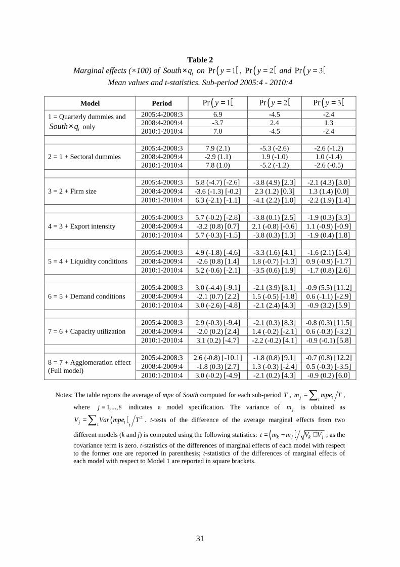
Table 2 Marginal effects (×100) of tSouth q× on ( )Pr y = 1 , ( )Pr y = 2 and ( )Pr y = 3

Mean values and t-statistics. Sub-period 2005:4 - 2010:4

Model Period ( )Pr y = 1 ( )Pr y = 2 ( )Pr y = 3

1 = Quarterly dummies and

tSouth q× only

2005:4-2008:3 6.9 -4.5 -2.4 2008:4-2009:4 -3.7 2.4 1.3 2010:1-2010:4 7.0 -4.5 -2.4

2 = 1 + Sectoral dummies 2005:4-2008:3 7.9 (2.1) -5.3 (-2.6) -2.6 (-1.2) 2008:4-2009:4 -2.9 (1.1) 1.9 (-1.0) 1.0 (-1.4) 2010:1-2010:4 7.8 (1.0) -5.2 (-1.2) -2.6 (-0.5)

3 = 2 + Firm size 2005:4-2008:3 5.8 (-4.7) [-2.6] -3.8 (4.9) [2.3] -2.1 (4.3) [3.0] 2008:4-2009:4 -3.6 (-1.3) [-0.2] 2.3 (1.2) [0.3] 1.3 (1.4) [0.0] 2010:1-2010:4 6.3 (-2.1) [-1.1] -4.1 (2.2) [1.0] -2.2 (1.9) [1.4]

4 = 3 + Export intensity 2005:4-2008:3 5.7 (-0.2) [-2.8] -3.8 (0.1) [2.5] -1.9 (0.3) [3.3] 2008:4-2009:4 -3.2 (0.8) [0.7] 2.1 (-0.8) [-0.6] 1.1 (-0.9) [-0.9] 2010:1-2010:4 5.7 (-0.3) [-1.5] -3.8 (0.3) [1.3] -1.9 (0.4) [1.8]

5 = 4 + Liquidity conditions 2005:4-2008:3 4.9 (-1.8) [-4.6] -3.3 (1.6) [4.1] -1.6 (2.1) [5.4] 2008:4-2009:4 -2.6 (0.8) [1.4] 1.8 (-0.7) [-1.3] 0.9 (-0.9) [-1.7] 2010:1-2010:4 5.2 (-0.6) [-2.1] -3.5 (0.6) [1.9] -1.7 (0.8) [2.6]

6 = 5 + Demand conditions 2005:4-2008:3 3.0 (-4.4) [-9.1] -2.1 (3.9) [8.1] -0.9 (5.5) [11.2] 2008:4-2009:4 -2.1 (0.7) [2.2] 1.5 (-0.5) [-1.8] 0.6 (-1.1) [-2.9] 2010:1-2010:4 3.0 (-2.6) [-4.8] -2.1 (2.4) [4.3] -0.9 (3.2) [5.9]

7 = 6 + Capacity utilization 2005:4-2008:3 2.9 (-0.3) [-9.4] -2.1 (0.3) [8.3] -0.8 (0.3) [11.5] 2008:4-2009:4 -2.0 (0.2) [2.4] 1.4 (-0.2) [-2.1] 0.6 (-0.3) [-3.2] 2010:1-2010:4 3.1 (0.2) [-4.7] -2.2 (-0.2) [4.1] -0.9 (-0.1) [5.8]

8 = 7 + Agglomeration effect (Full model)

2005:4-2008:3 2.6 (-0.8) [-10.1] -1.8 (0.8) [9.1] -0.7 (0.8) [12.2] 2008:4-2009:4 -1.8 (0.3) [2.7] 1.3 (-0.3) [-2.4] 0.5 (-0.3) [-3.5] 2010:1-2010:4 3.0 (-0.2) [-4.9] -2.1 (0.2) [4.3] -0.9 (0.2) [6.0]

Notes: The table reports the average of mpe of South computed for each sub-period T , j ttm mpe T=∑ ,

where ,...,j = 1 8 indicates a model specification. The variance of jm is obtained as

( )j tt tV Var mpe T=∑ 2 . t-tests of the difference of the average marginal effects from two

different models (k and j) is computed using the following statistics: ( )k j k jt m m V V= − + , as the

covariance term is zero. t-statistics of the differences of marginal effects of each model with respect to the former one are reported in parenthesis; t-statistics of the differences of marginal effects of each model with respect to Model 1 are reported in square brackets.

32

Table 3 Cross correlations between the relative frequencies of assessment on production levels in

the North-Center and South

Period 0 1 2 3 4

2003:2 – 2010:4 lead

0.94 0.85 0.69 0.54 0.41

lag 0.85 0.72 0.60 0.49

2005:4 – 2010:4 lead

0.95 0.86 0.68 0.53 0.36

lag 0.87 0.73 0.61 0.50

33

Table 4 Model comparison. Log-likelihood, AIC, BIC and R2 measures. Sub-period 2005:4 -

2010:4

Model Log-lik. AIC BIC R2_AN R2_M

1 = Quarterly dummies and tSouth q× only -161,077 322,243 322,693 0.088 0.093

2 = 1 + Sectoral dummies

-160,967 322,059 322,704 0.089 0.094

3 = 2 + Firm size -160,359 320,868 321,636 0.094 0.099

4 = 3 + Export intensity -160,234 320,630 321,460 0.095 0.100

5 = 4 + Liquidity conditions and expectations

-145,490 291,159 292,064 0.122 0.130

6 = 5 + Demand conditions and expectations

-135,011 270,225 271,252 0.199 0.220

7 = 6 + Capacity utilization

-134,617 269,445 270,513 0.201 0.223

8 = 7 + Agglomeration effects (Full model)

-132,409 265,033 266,119 0.202 0.224

Notes: R2_AN is Aldrich and Nelson (1984) R2 measure, R2_AN is Maddala (1983) R2 measure

34

Table 5 Descriptive statistics

Sub-period 2005:4 - 2010:4

North

Min Q(25%) median Q(75%) Q(90%) Max mean Std. dev.

Skew.

Firm size 5 10 20 55 170 20,048 85.3 333.1 20.3 Export intensity 0 0 0 33 70 100 19.0 27.8 1.3

South

Min Q(25%) Median Q(75%) Q(90%) Max mean Std. dev.

Skew.

Firm size 5 9 15 32 85 7,545 49.3 253.5 20.5 Export intensity 0 0 0 3 30 100 8.2 19.6 2.7

Percentage of firms

North South

Liquidity conditions Good 30.7 23.5 Mediocre 55.2 56.3 Bad 14.0 20.3

Expectations on liquidity conditions Better 11.6 14.8 Equal 72.2 69.2 Worse 16.2 16.0

Domestic demand conditions High 9.7 8.4 Normal 54.6 56.8 Low 35.7 34.8

Foreign demand conditions High 6.0 3.0 Normal 28.7 17.3 Low 19.9 12.5

Expected demand conditions Increase 24.5 31.3 Stationarity 60.0 54.8 Decrease 15.5 13.8

Capacity utilization Excess 32.6 30.8 Around normal 60.8 62.4 Below normal 6.6 6.9

Total number of firms 149,139 49,086

35

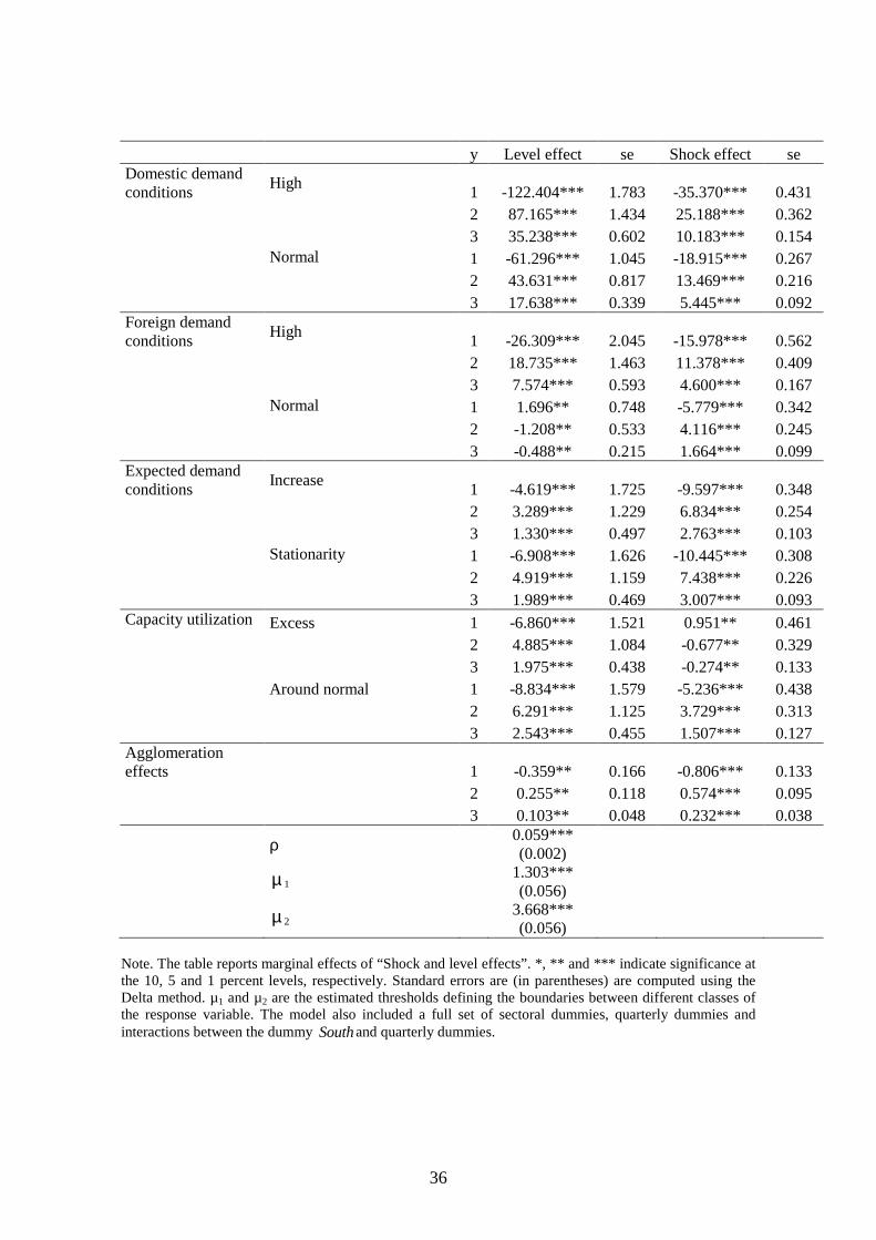
Table 6 mpe (×100) of “shock and level effects” RE-ORM (Full Model 8). Sub-period 2005:4 - 2010:4

y Level effect se Shock effect Se Firm size Ln emp (2005:4-2008:3) 1 -4.399*** 0.665 -12.701*** 2.331 2 3.132*** 0.474 9.044*** 1.661 3 1.266*** 0.192 3.656*** 0.672 Ln emp2 (2005:4-2008:3) 1 0.520*** 0.083 0.001 0.334 2 -0.370*** 0.059 -0.001 0.238 3 -0.150*** 0.024 0.000 0.096 Ln emp (2008:4-2009:4) 1 -1.173 0.924 -8.821*** 2.933 2 0.836 0.658 6.282*** 2.089 3 0.338 0.266 2.540*** 0.845 Ln emp2 (2008:4-2009:4) 1 0.344*** 0.117 -0.020 0.420 2 -0.245*** 0.083 0.014 0.299 3 -0.099*** 0.034 0.006 0.121 Ln emp (2010:1-2010:4) 1 -2.599** 1.002 -15.139*** 3.150 2 1.851** 0.714 10.781*** 2.245 3 0.748** 0.289 4.358*** 0.908 Ln emp2 (2010:1-2010:4) 1 0.441*** 0.125 1.400*** 0.431 2 -0.314*** 0.089 -0.997*** 0.307 3 -0.127*** 0.036 -0.403*** 0.124 Export intensity 2005:4-2008:3 1 -0.055*** 0.010 -0.072*** 0.012 2 0.039*** 0.007 0.051*** 0.009 3 0.016*** 0.003 0.021*** 0.003 2008:4-2009:4 1 -0.011 0.013 -0.088*** 0.019 2 0.008 0.009 0.063*** 0.013 3 0.003 0.004 0.025*** 0.005 2010:1-2010:4 1 -0.073*** 0.014 -0.105*** 0.020 2 0.052*** 0.010 0.075*** 0.014 3 0.021*** 0.004 0.030*** 0.006 Liquidity conditions

Good 1 -3.730*** 0.956 -6.332*** 0.418

2 2.656*** 0.681 4.509*** 0.299

3 1.074*** 0.276 1.823*** 0.121

Mediocre 1 -3.615*** 0.994 -3.645*** 0.337

2 2.574*** 0.708 2.595*** 0.241

3 1.041*** 0.287 1.049*** 0.097 Expectations on liquidity conditions

Better 1 -6.246*** 1.682 -17.214*** 0.413

2 4.448*** 1.199 12.259*** 0.309

3 1.798*** 0.485 4.956*** 0.127 Equal 1 -1.776 1.262 -11.517*** 0.307 2 1.265 0.899 8.201*** 0.228 3 0.511 0.363 3.315*** 0.093

36

y Level effect se Shock effect se Domestic demand conditions

High 1 -122.404*** 1.783 -35.370*** 0.431

2 87.165*** 1.434 25.188*** 0.362

3 35.238*** 0.602 10.183*** 0.154

Normal 1 -61.296*** 1.045 -18.915*** 0.267

2 43.631*** 0.817 13.469*** 0.216

3 17.638*** 0.339 5.445*** 0.092 Foreign demand conditions

High 1 -26.309*** 2.045 -15.978*** 0.562

2 18.735*** 1.463 11.378*** 0.409

3 7.574*** 0.593 4.600*** 0.167

Normal 1 1.696** 0.748 -5.779*** 0.342

2 -1.208** 0.533 4.116*** 0.245

3 -0.488** 0.215 1.664*** 0.099 Expected demand conditions

Increase 1 -4.619*** 1.725 -9.597*** 0.348

2 3.289*** 1.229 6.834*** 0.254

3 1.330*** 0.497 2.763*** 0.103 Stationarity 1 -6.908*** 1.626 -10.445*** 0.308 2 4.919*** 1.159 7.438*** 0.226 3 1.989*** 0.469 3.007*** 0.093 Capacity utilization Excess 1 -6.860*** 1.521 0.951** 0.461 2 4.885*** 1.084 -0.677** 0.329 3 1.975*** 0.438 -0.274** 0.133 Around normal 1 -8.834*** 1.579 -5.236*** 0.438 2 6.291*** 1.125 3.729*** 0.313 3 2.543*** 0.455 1.507*** 0.127 Agglomeration effects 1 -0.359** 0.166 -0.806*** 0.133 2 0.255** 0.118 0.574*** 0.095 3 0.103** 0.048 0.232*** 0.038 ρ 0.059***

(0.002) µ 1

1.303*** (0.056)

µ 2 3.668*** (0.056)

Note. The table reports marginal effects of “Shock and level effects”. *, ** and *** indicate significance at the 10, 5 and 1 percent levels, respectively. Standard errors are (in parentheses) are computed using the Delta method. µ1 and µ2 are the estimated thresholds defining the boundaries between different classes of the response variable. The model also included a full set of sectoral dummies, quarterly dummies and interactions between the dummy Southand quarterly dummies.

37

Figure 1 - Cyclical component of the industrial production index and marginal probability effects of quarterly dummies

38

Figure 2 - Marginal effects of South

39

Figure A1 - Italy’s Industrial Production index

Time

1970 1980 1990 2000 2010

6080

100

120

Baxter-King Filter of Production_index

1990 1995 2000 2005 2010

8590

9510

010

5 Production_index trend

Cyclical component (deviations from trend)

1990 1995 2000 2005 2010

-10

-50

510

40

Figure A2 - Marginal effects of South