I

First Young Researchers Workshop “Physics Challenges in the LHC Era”

2009

II

FRASCATI PHYSICS SERIES Series Editor Danilo Babusci Technical Editor Luigina Invidia Cover by Claudio Federici

Volume XLVIII

Istituto Nazionale di Fisica Nucleare – Laboratori Nazionali di Frascati Divisione Ricerca SIDS – Servizio Informazione e Documentazione Scientifica Ufficio Biblioteca e Pubblicazioni P.O. Box 13, I–00044 Frascati Roma Italy email: sis.publications@lnf.infn.it

III

IV

FRASCATI PHYSICS SERIES First Young Researchers Workshop “Physics Challenges in the LHC Era” 2009 Copyright © 2009 by INFN All rights reserved. No part of this publication may be reproduced, stored in a retrieval system or transmitted, in any form or by any means, electronic, mechanical, photocopying, recording or otherwise, without the prior permission of the copyright owner. ISBN 978–88–86409–57–5

V

FRASCATI PHYSICS SERIES

Volume XXXVIII

First Young Researchers Workshop “Physics Challenges in the LHC Era”

2009

Editor Enrico Nardi

Frascati, May 11th and May 14th, 2009

VI

International Advisory Committee G. Altarelli Università Roma Tre W. Buchmuller DESY F. Ceradini Università Roma Tre A. Di Ciaccio Università Roma Tor Vergata J. Ellis CERN B. Grinstein University of California San Diego R. Fiore Università della Calabria

Local Organizing Committee M. Antonelli INFN Frascati, D. Aristizabal INFN Frascati O. Cata INFN Frascati V. Del Duca INFN Frascati R. Faccini Università Roma La Sapienza e INFN Roma G. Isidori INFN Frascati J. F. Kamenik INFN Frascati e JSI E. Nardi INFN Frascati (Chair) M. Palutan INFN Frascati F. Terranova INFN Frascati

VII

PREFACE

The first Young Researcher Workshop "Physics Challenges in the LHC Era" was held in the Frascati Laboratories during May 11th and 14th 2009, in conjunction with the XIV Frascati Spring School "Bruno Touschek".

The main goal of the Workshop was to provide an opportunity for the students attending the Spring School to play an active role in complementing the scientific program by giving short lectures to their colleagues on their specific research topics. In this way the students learn how to organize a presentation on a specialistic subject, so that it will be understandable by an audience of young physicists in the training stage, and how to condense the results of months of research work within a fifteen minutes talk. Helping to develop these skills is an integral part of the scientific formation the Spring School is aiming to.

The Workshop was very successful, both in its scientific and formative aspects. Despite that for many of the sixteen young speakers this was the first public presentation of their researches, all the talks reflected a remarkably high professional level, and could have well fitted within the scientific program of many international conferences.

These proceedings, that collect the joint efforts of the speakers of the Young Researchers Workshop, aim to set a benchmark for the scientific level required to participate in future editions of the Workshop. It will also provide useful guidelines for structuring the presentations of our next set of young lecturers.

Too many people contributed to the success of the Young Researcher Workshop "Physics Challenges in the LHC Era" and of the joint XIV Frascati Spring School "Bruno Touschek" to give here a complete list. However, a special acknowledgment must be given to the Workshop secretariat staff and backbones of the Frascati Spring School Maddalena Legramante and Angela Mantella, to Claudio Federici, that put a special effort in realizing the graphics of the Workshop and School posters, to Luigina Invidia for the technical editing of these proceedings, and to the Director of the Frascati Laboratories Mario Calvetti for constant encouragement and support. Frascati, July 2009 Enrico Nardi

VIII

Artwork by Claudio Federici

IX

CONTENTS Preface ................................................................................................ VII Aleksey Reznichenko QCD amplitudes with the gluon exchange at high energies

(and gluon Reggeization proof) ................................................1 Paolo Lodone Including QCD radiation corrections in transplanckian

scattering ...................................................................................7 Luis A. Muñoz Purely flavored leptogenesis at the TeV scale ......................13 Pablo Roig Hadronic τ decays into two and three meson modes within resonance chiral theory ...............................................19 Giovanni Siragusa Measurement of the missing transverse energy in the ATLAS detector.......................................................................25 Roberto Di Nardo Measurement of the pp → Z →µµ + X cross section at LHC with ATLAS experiment..............................................31 Manuela Venturi Study of the geometrical acceptance for vector bosons in

ATLAS and its systematic uncertainty..................................37 Giorgia Mila The CMS muon reconstruction .............................................43 Antonio E. Cárcamo Heavy vector pair production at LHC in the chiral Lagrangian formulation............................................................49 Mark Round Mass degenerate heavy vector mesons at Hadron Colliders ....................................................................55 Anna Vinokurova Study of B → Kηc and B → Kηc (2S) decays ...................61 T. Danger Julius Continuum suppression in the reconstruction of B0 → π0 π0 ............................................................................67 Daniela Bagliani A microcalorimeter measurement of the neutrino mass,

studying 187Re single β decay and 163Ho electron-capture decay .............................................................73 Roberto Iuppa Measurement of the antiproton/proton ratio at few-TeV energies with the ARGO-YBJ experiment ............79 Anastasia Karavdina Event reconstruction in the drift chamber of the CMD-3 detector ......................................................................85 Shinji Okada Kaonic atoms at DAΦNE ..................................................... 91

Frascati Physics Series Vol. XLVIII (2009), pp. 1-6Young Researchers Workshop: “Physics Challenges in the LHC Era”

Frascati, May 11 and 14, 2009

QCD AMPLITUDES WITH THE GLUON EXCHANGE ATHIGH ENERGIES

(AND GLUON REGGEIZATION PROOF)

A.V. ReznichenkoBudker Institute of Nuclear Physics, 630090 Novosibirsk, Russia

M.G. KozlovNovosibirsk State University, 630090 Novosibirsk, Russia

Abstract

We demonstrate that the multi-Regge form of QCD amplitudes with gluonexchanges is proved in the next-to-leading approximation. The proof is basedon the bootstrap relations, which are required for the compatibility of thisform with the s-channel unitarity. It was shown that the fulfillment of all theserelations ensures the Reggeized form of energy dependent radiative correctionsorder by order in perturbation theory. Then we prove that all these relations arefulfilled if several bootstrap conditions on the Reggeon vertices and trajectoryhold true. All these conditions are checked and proved to be satisfied for allpossible t-channel color representations. That finally completes the proof ofthe gluon Reggeization in the next-to-leading approximation and provides thefirm basis for BFKL approach therein.

1

1 Introduction

Reggeization of gluons as well as quarks is one of remarkable properties of

Quantum Chromodynamics (QCD). The gluon Reggeization is especially im-

portant since cross sections non vanishing in the high energy limit are related

to gluon exchanges in cross channels. A primary Reggeon in QCD turns out

to be the Reggeized gluon.

The gluon Reggeization gives the most common basis for the description of

high energy processes. In particular, the famous BFKL equation 1) was derived

supposing the Reggeization. The most general approach to the unitarization

problem is the reformulation of QCD in terms of a gauge-invariant effective

field theory for the Reggeized gluon interactions.

The gluon Reggeization was proved in the leading logarithmic approxi-

mation (LLA), i.e. in the case of summation of the terms (αS ln s)n in cross-

sections of processes at energy√

s in the c.m.s., but till now remains a hypoth-

esis in the next-to-leading approximation (NLA), when the terms αS(αS ln s)n

are also kept. Now the BFKL approach 1), based on the gluon Reggeization,

is intensively developed in the NLA.

We present the proof of the gluon Reggeization in the NLA. Substan-

tially in our consideration we follow the paper 2). All references are presented

therein. First we show that the fulfillment of the bootstrap relations guarantees

the multi–Regge form of QCD amplitudes. Then we demonstrate that an infi-

nite set of these bootstrap relations are fulfilled if several conditions imposed

on the Reggeon vertices and the trajectory (bootstrap conditions) hold true.

Now almost all these conditions are proved to be satisfied. In our consideration

we hold the following terminology:

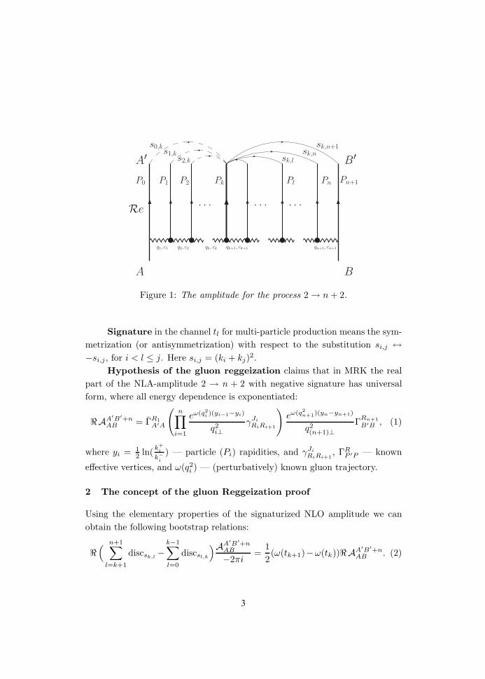
Multi-Regge kinematics (MRK). Let us consider the amplitude (see

fig.1) A2→n+2 of the process A + B → A′ + J1 + . . . + Jn + B′: see the fig-

ure. We use light-cone momenta n1 and n2, with n21 = n2

2 = 0, (n1n2) = 1,

and denote (pn2) ≡ p+, (pn1) ≡ p−. Let assume that initial momenta pA

and pB have predominant components p+A and p−B. MRK supposes that ra-

pidities of final jets Ji with momenta ki yi = 12 ln(k+

i /k−

i

)decrease with i:

y0 > y1 > . . . > yn > yn+1; as for y0 and yn+1, it is convenient to define

them as y0 = yA ≡ ln(√

2p+A/|q1⊥|

)and yn+1 = yB ≡ ln

(|q(n+1)⊥|/√

2p−B).

Notice that qi indicate the Reggeon momenta and q1 = pA′ − pA ≡ qA,

qn+1 = pB − pB′ ≡ qB.

2

A′

A

B′

B

. . . . . . . . .

sk,n+1sk,n

sk,l

s0,ks1,k

s2,k

P0

q1, c1 q2, c2 qk, ck qk+1, ck+1

P1 P2 Pk Pl Pn Pn+1

qn+1, cn+1

Re

Figure 1: The amplitude for the process 2 → n + 2.

Signature in the channel tl for multi-particle production means the sym-

metrization (or antisymmetrization) with respect to the substitution si,j ↔−si,j, for i < l ≤ j. Here si,j = (ki + kj)

2.

Hypothesis of the gluon reggeization claims that in MRK the real

part of the NLA-amplitude 2 → n + 2 with negative signature has universal

form, where all energy dependence is exponentiated:

AA′B′+nAB = ΓR1

A′A

(n∏

i=1

eω(q2i )(yi−1−yi)

q2i⊥

γJi

RiRi+1

)eω(q2

n+1)(yn−yn+1)

q2(n+1)⊥

ΓRn+1

B′B , (1)

where yi = 12 ln(

k+

i

k−

i

) — particle (Pi) rapidities, and γJi

RiRi+1, ΓR

P ′P — known

effective vertices, and ω(q2i ) — (perturbatively) known gluon trajectory.

2 The concept of the gluon Reggeization proof

Using the elementary properties of the signaturized NLO amplitude we can

obtain the following bootstrap relations:

( n+1∑

l=k+1

discsk,l−

k−1∑l=0

discsl,k

)AA′B′+nAB

−2πi=

1

2(ω(tk+1)−ω(tk))AA′B′+n

AB . (2)

3

. . .

J1Jj−1

γJj−1Rj−1Rj

〈JjRj|

JjA′

A

Jn

B

. . .︷ ︸︸ ︷ ︷ ︸︸ ︷

B′

|B′B〉

JnJj+1

Jj+1

. . . . . .. . .

eKYj+1 eKYn+1

γJ1R1R2

ΓR1A′A

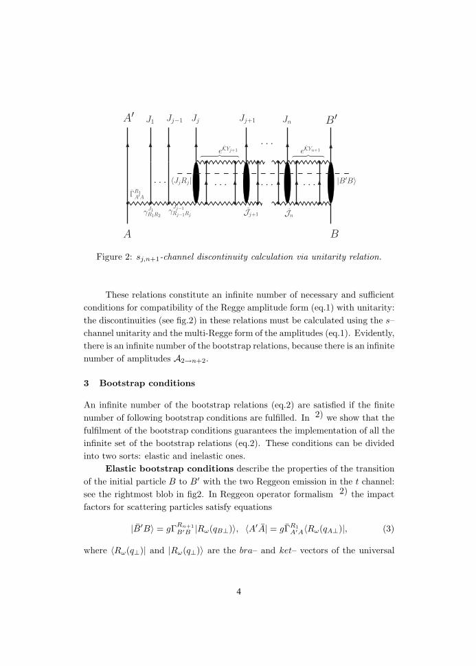
Figure 2: sj,n+1-channel discontinuity calculation via unitarity relation.

These relations constitute an infinite number of necessary and sufficient

conditions for compatibility of the Regge amplitude form (eq.1) with unitarity:

the discontinuities (see fig.2) in these relations must be calculated using the s–

channel unitarity and the multi-Regge form of the amplitudes (eq.1). Evidently,

there is an infinite number of the bootstrap relations, because there is an infinite

number of amplitudes A2→n+2.

3 Bootstrap conditions

An infinite number of the bootstrap relations (eq.2) are satisfied if the finite

number of following bootstrap conditions are fulfilled. In 2) we show that the

fulfilment of the bootstrap conditions guarantees the implementation of all the

infinite set of the bootstrap relations (eq.2). These conditions can be divided

into two sorts: elastic and inelastic ones.

Elastic bootstrap conditions describe the properties of the transition

of the initial particle B to B′ with the two Reggeon emission in the t channel:

see the rightmost blob in fig2. In Reggeon operator formalism 2) the impact

factors for scattering particles satisfy equations

|B′B〉 = gΓRn+1

B′B |Rω(qB⊥)〉, 〈A′A| = gΓR1

A′A〈Rω(qA⊥)|, (3)

where 〈Rω(q⊥)| and |Rω(q⊥)〉 are the bra– and ket– vectors of the universal

4

(process independent) eigenstate of the BFKL kernel K with the eigenvalue

ω(q⊥),

K|Rω(q2⊥

)〉 = ω(q2⊥

)|Rω(q⊥)〉, 〈Rω(q2⊥

)|K = 〈Rω(q⊥)|ω(q2⊥

), (4)

The last equations give us elastic bootstrap conditions. The bootstrap condi-

tions (eq.3) and (eq.4) are known since a long time and have been proved to

be satisfied about ten years ago.

Inelastic bootstrap conditions connect the Reggeon-gluon impact fac-

tors (the leftmost blob in fig.2) and the gluon production operator (the centre

blobs in fig.2). In our formalism these conditions can be written in the following

universal form:

Ji |Rω(q(i+1)⊥)〉 g q2(i+1)⊥ + |JiRi+1〉 = |Rω(qi⊥)〉 g γJi

RiRi+1. (5)

The first term is referred to as the operator of the jet Ji production. In

our approximation (NLA) the jet Ji is either one gluon, or quark-antiquark

pair (or two gluons) with close rapidities. The operator of the jet produc-

tion 〈G′1G′

2|Ji |Rω(q(i+1)⊥)〉 (i.e. operator Ji projected onto the two-Reggeon

t-channel state 〈G′

1G′

2| and onto kernel eigenstate |Rω(qi⊥)〉) can be explicitly

viewed 2) through known in NLO effective vertices and the gluon trajectory.

The second element 〈G′

1G′

2|JiRi+1〉 of (eq.5) is the impact-factor of the jet pro-

duction. It describes the transition of the t-channel Reggeon Ri+1 into the

final jet Ji and two-Reggeon t-channel state. The analytical form through the

effective vertices and the trajectory one can find in 2). For the case when the

jet Ji is quark-antiquark pair or two gluons the bootstrap condition (eq.5) was

proved several years ago 3). The last unproved bootstrap condition reproduces

the case when Ji is one gluon.

From the explicit form of the effective vertices it is easy to see that for the

gluon contribution there are only three independent colour structures that lead

to the nontrivial bootstrap condition. The optimal choice is the “trace-based”:

Tr[T c2T aT c1T i], Tr[T aT c2T c1T i], Tr[T aT c1T c2T i], (6)

where a is a colour index of the external gluon; i is a colour index of one-Reggeon

t-channel state, and c1, c2 are colour indices of the two-Reggeon t-channel state.

Two years ago by the direct loop calculation we demonstrated that the inelastic

bootstrap condition was fulfilled being projected onto the colour octet in the

5

t-channel. For the quark contribution all bootstrap conditions can be obtained

from the octet one and thereby are fulfilled.

The bootstrap conditions for the second and third colour structures in

(eq.6) can be obtained from the octet one in a simple way. The first colour

structure (symmetric with respect to c1 and c2) is essentially new.

Up to date by the direct loop calculation in the dimensional regulariza-

tion we found both impact-factor and operator of the gluon production, and

checked the cancellation of all singular (collinear and infrared singularities),

logarithmic, and rational terms within the bootstrap condition for this struc-

ture. The matter of the nearest future is to cancel all dilogarithmic and double

logarithmic terms. That will accomplish the NLA gluon reggeization proof

irreversibly.

4 Conclusion

We presented the basic steps of the proof that in the multi–Regge kinematics

real parts of QCD amplitudes for processes with gluon exchanges have the

simple multi-Regge form.

The proof is based on the bootstrap relations required by the compat-

ibility of the multi–Regge form (eq.1) of inelastic QCD amplitudes with the

s–channel unitarity.

References

1. V.S. Fadin, E.A. Kuraev and L.N. Lipatov, Phys. Lett. B 60, 50 (1975).

2. V.S. Fadin, R. Fiore, M.G. Kozlov, A.V. Reznichenko, Phys. Lett. B, 639

(2006)

3. V.S. Fadin, M.G. Kozlov and A.V. Reznichenko, Yad. Fiz. 67, 377 (2004).

6

Frascati Physics Series Vol. XLVIII (2009), pp. 7-12Young Researchers Workshop: “Physics Challenges in the LHC Era”

Frascati, May 11 and 14, 2009

INCLUDING QCD RADIATION CORRECTIONSIN TRANSPLANCKIAN SCATTERING

Paolo LodoneScuola Normale Superiore of Pisa and INFN

Abstract

The hypothesis of models with Large Extra Dimensions is that the fundamentalPlanck scale can be lowered down to some TeV if gravity propagates in some(compactified) extra dimensions. If this is the case, quantum gravity effects

could be visible at the LHC. Gian F. Giudice et al in 1) studied these effectsin the eikonal approximation. It is interesting both from a phenomenologicaland a theoretical point of view to study the corrections to these results due tothe QCD radiation. To evaluate this contribution, we generalize a shock-wavemethod proposed by ’t Hooft, so that we are able to obtain the amplitude atfirst order in QCD corrections but resummed at all orders in gravity. Studyingthis result we can learn many interesting things, for example we can extractthe true scale of the process. This is actually work in progress jointly with

Vyacheslav Rychkov, the complete results will appear in 2).

7

1 Introduction

The hypothesis 3) of Large Extra Dimensions (LED) is motivated by the

Hierarchy problem and amounts to suppose that there exists n compactified

extra dimensions so that the Einstein - Hilbert action of General Relativity

(GR) becomes, with D = 4 + n:

SD =1

2

∫dDx

√−g(D)Mn+2

D R(D). (1)

Integrating out these extra dimensions we obtain:

M2Pl = M2+n

D (2πr)n (2)

where r is the size of the extra dimensions in the simplest case of toroidal

compactification. This means that if the volume of the compactified extra

dimensions is “large”, then the scale MD at which Quantum Gravity (QG)

should manifest itself is much lower then the usual Planck scale MPl.

The important point (see 4) for a review) is that if we assume that

only gravity can propagate in the n extra dimensions, then the only observable

effect is a deviation from the newtonian potential at distances smaller than

r. Moreover setting MD = 1 TeV we have r = 2 · 10−161032n mm. Since the

experimental data impose r ≤ 0.2 mm, we immediatly see that:

n ≥ 2 , MD ≈ 1 TeV (3)

is a serious possibility which has to be taken into account at the LHC.

2 Transplanckian scattering

Let us consider the case of scattering events, following 1). Defining the D-

dimensional gravitational coupling constant as GD = (2π)n−1

n+1

4cn−1Mn+2

D

, the relevant

length scales are:

λB =4πc√

s, λP =

(GD

c3

) 1n+2

, RS =1√π

[8Γ(n+3

2 )

n + 2

] 1n+1

(4)

where λB is the de Broglie wavelength, λP is the Planck scale (at which QG

appears), and RS is the Schwarzschild radius (at which curvature effects become

8

large). It is important to notice that in this D-dimensional framework we also

have the length scale:

bc =

(GDs

c5

) 1n

(5)

which can not be defined if n = 0 and moreover goes to infinity if → 0 with

GD fixed. This means that bc is related to the size of the classical region in the

impact parameter space.

Since the true theory of QG is not known, we are interested in model

independent predictions. First of all let us assume that bc RS , which is

certainly true at sufficiently high energy. Notice that for impact parameter

b RS gravity can be linearized. Moreover if√

s MD then RS λP λB, which means that QG effects are expected to be small. Finally, in the

case of forward scattering at small angles, we are able to perform a predictive

computation using the eikonal resummation or the shock-wave method, as we

will see in the following sections. In conclusion, in the transplanckian eikonal

regime defined by: √s MD ,

−t

s 1 (6)

it is possible to obtain model independent predictions which rely only on Quan-

tum Mechanics (QM) and linearized GR. Notice that all this can be of interest

only in a LED scenario with the QG scale MD lowered down to a few TeV.

3 Eikonal amplitude without radiation

As shown in 1) and 5), a first approach for the evaluation of the transplanck-

ian eikonal amplitude is “eikonalization”, which amounts to resum an infinite

number of Feynman diagrams with graviton exchanges which are one by one

ultraviolet (UV) divergent but whose sum is finite. In performing this sum we

neglect the virtuality of gravitons in the matter propagators and we make use

of the on-shell vertices. The final result is:

Aeik(q⊥) = −2is

∫d2b⊥eiq⊥b⊥(eiχ(b⊥) − 1) (7)

where q⊥ is the momentum transfer, which is mainly transverse (q2⊥

≈ −t),

and:

χ(b⊥) =1

2s

∫d2q⊥(2π)2

e−iq⊥b⊥Atree(q⊥) =

(bc

b⊥

)n

. (8)

9

Notice that this amplitude is spin independent and moreover there is no UV

sensitivity. This means that in this regime we can obtain a prediction in per-

turbative QG which does not depend on the way QG is regolarized.

An equivalent approach which shows even more explicity the fact that this

prediction relies only on QM and GR is ’t Hooft shock wave method 6). In

this case we solve the Einstein equations for a very energetic particle, obtaining

the Aichelburg-Sexl shock wave metric 7):

ds2 = −dx+dx− + Φ(x⊥)δ(x−)(dx−)2 + dx2⊥ (9)

where the particle is moving in the positive z direction, and:

Φ

8πGD

= −E

πlog |x⊥| if D = 4

=2 Γ(k+1

2 )E

2 πk+1

2 (D − 4) |x⊥|D−4if D > 4 . (10)

We can perform a (discontinuous) coordinate transformation x → x′ in order

to make the metric continuous across x− = 0. At x− = x′− = 0 we have:x+ = x′+ + θ(x−)Φ(x⊥)xi = x′i (i = 1, 2) .

(11)

Then we solve the equations of motion for the other particle in this shock-wave

spacetime, which consists of two flat semispaces glued together at x− = 0 with

the discontinuity (11). For a particle with energy E moving in the negative z

direction (p = (E,−E, 0)) the wavefuction is, before the collision:

ψ(x) = e−ipx = e−iEx+

(x− < 0) (12)

while immediatly after the collision the continuity in the x′ coordinates implies:

ψ(x) = e−iE(x+−Φ(x⊥)) (x− → 0+) (13)

thus we obtain the eikonal amplitude:

Aeik(x⊥) = eiEΦ(x⊥). (14)

It can be checked 2) that EΦ(x⊥) is exactly the eikonal χ(x⊥) of (8). Notice

that the −1 in (7) gives a contribution proportional to δ(q⊥), and the overall

factors can be obtained by properly normalizing the wavefunctions.

10

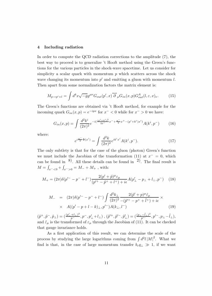
4 Including radiation

In order to compute the QCD radiation corrections to the amplitude (7), the

best way to proceed is to generalize ’t Hooft method using the Green’s func-

tions for the various particles in the shock-wave spacetime. Let us consider for

simplicity a scalar quark with momentum p which scatters across the shock

wave changing its momentum into p′ and emitting a gluon with momentum l.

Then apart from some normalization factors the matrix element is:

Mp→p′+l =

∫d4x

√−ggµνGout(p′, x)

←→∂ µGin(x, p)GA

out(l, ε, x)ν . (15)

The Green’s functions are obtained via ’t Hooft method, for example for the

incoming quark Gin(x, p) = e−ipx for x− < 0 while for x− > 0 we have:

Gin(x, p) =

∫d2ki

(2π)2e−i( (pi+ki)2

2p−x−+ p−

2x+

−(pi+ki)xi)A(ki, p−) (16)

where:

ei p−

2Φ(xi) =

∫d2k

(2π)2eikixi

A(ki, p−). (17)

The only subtlety is that for the case of the gluon (photon) Green’s function

we must include the Jacobian of the transformation (11) at x− = 0, which

can be found in 8). All these details can be found in 2). The final result is

M =∫

x−<0+∫

x−>0= M− + M+ , with:

M+ = (2π)δ(p′− − p− + l−)2(p′ + p)µεµ

(p′+ − p+ + l+) + iεA(p′

⊥− p⊥ + l⊥, p−) (18)

M− = (2π)δ(p′− − p− + l−)

∫d2k⊥(2π)2

2(p′ + p)µεµ

−(p′+ − p+ + l+) + iε×

× A((p′ − p + l − k)⊥, p′−)A(k⊥, l−) (19)

(p+, p−, p⊥) = ((p′

⊥+l⊥)2

p−, p−, p′

⊥+l⊥) , (p′+, p′−, p′

⊥) = ( (p⊥−l⊥)2

p′−, p′−, p⊥− l⊥),

and εµ is the transformed of εµ through the Jacobian of (11). It can be checked

that gauge invariance holds.

As a first application of this result, we can determine the scale of the

process by studying the large logarithms coming from∫

d2l |M |2. What we

find is that, in the case of large momentum transfer bcq⊥ 1, if we want

11

to reabsorb the large corrections the scale at which the parton distribution

functions must be normalized is:

Qeff =(q⊥bc)

1n+1

bc

. (20)

Notice that for n = 0 the scale lenght bc cannot be defined, and in fact in

this case there is no “strange behaviour”. It is interesting to note also that

this scale is essentially the inverse of the impact parameter that dominates the

amplitude (7) in the stationary phase approximation, which is named bs in 1).

5 Conclusions and perspectives

For the moment the main result of this study is the generalization of ’t Hooft

method 6) in order to include QCD radiation in transplanckian scattering. The

sum of (18) and (19), apart from some normalization factors, gives Mp→p′+l

at the first order in QCD and at all orders in gravity in the regime (6). We

have also hints about the true scale of this process, which may not be just the

momentum transfer. In 2) we will derive all this in full detail and we will

carefully study the implications for signals at colliders.

6 Acknowledgements

In this project I am working jointly with Vyacheslav Rychkov, whom I thank.

References

1. G.F. Giudice et al, Nucl. Phys. B 630 293-325 (2002).

2. P. L., V. Rychkov, QCD Radiation in transplanckian scattering, to appear.

3. N. Arkani-Hamed et al, Phys. Lett. B 429, 263 (1998).

4. C. Csaki, [arXiv:hep-ph/0404096]; G.D. Kribs, [arXiv:hep-ph/0605325].

5. D. Kabat et al, Nucl. Phys. B 388, 570 (1992).

6. G. ’t Hooft, Phys. Lett. B 198, 61 (1897).

7. P.C. Aichelburg et al, Gen. Rel. Grav. 2, 303 (1971).

8. V. Rychkov, Phys. Rev. D 70 044003 (2004).

12

Frascati Physics Series Vol. XLVIII (2009), pp. 13-18Young Researchers Workshop: “Physics Challenges in the LHC Era”

Frascati, May 11 and 14, 2009

PURELY FLAVORED LEPTOGENESIS AT THE TeV SCALE

Luis Alfredo MunozInstituto de Fısica, Universidad de Antioquia, A.A. 1226, Medellın, Colombia

Abstract

I study variations of the standard leptogenesis scenario that can arise if anadditional mass scale related to the breaking of some new symmetry is presentbelow the mass MN1

of the lightest right-handed Majorana neutrino. I presenta particular realization of this scheme that allows for leptogenesis at the TeVscale. In this realization the baryon asymmetry is exclusively due to flavoreffects.

1 Introduction

From observations of light element abundances and of the Cosmic microwave

background radiation 1) the Cosmic baryon asymmetry, YB = nB−nB

s=

(8.75 ± 0.23) × 10−10, (where s is the entropy density) can be inferred. The

conditions for a dynamical generation of this asymmetry (baryogenesis) are

13

well known 2) and depending on how they are realized different scenarios for

baryogenesis can be defined (see ref. 3) for a througout discussion). Lep-

togenesis 4) is a scenario in which an initial lepton asymmetry, generated

in the out-of-equilibrium decays of heavy singlet Majorana neutrinos (Nα), is

partially converted in a baryon asymmetry by anomalous sphaleron interac-

tions 5) that are standard model processes. Singlet Majorana neutrinos are

an essential ingredient for the generation of light neutrino masses through the

seesaw mechanism 6). This means that if the seesaw is the source of neutrino

masses then qualitatively, leptogenesis is unavoidable. Consequently, whether

the baryon asymmetry puzzle can be solved within this framework turn out

to be a quantitative question. This has triggered a great deal of interest on

quantitative analysis of the standard leptogenesis model and indeed a lot of

progress during the last years has been achieved (see ref. 7)).

2 The Model

The model we consider here 8) is a simple extension of the standard model

containing a set of SU(2)L × U(1)Y fermionic singlets, namely three right-

handed neutrinos (Nα = NαR + N cαR) and three heavy vectorlike fields (Fa =

FaL + FaR). In addition, we assume that at some high energy scale, taken to

be of the order of the leptogenesis scale MN1, an exact U(1)X gauge horizontal

symmetry forbids direct couplings of the lepton i and Higgs Φ doublets to the

heavy Majorana neutrinos Nα. At lower energies, U(1)X gets spontaneously

broken by the vacuum expectation value (vev) σ of a SU(2) singlet scalar field

S. Accordingly, the Yukawa interactions of the high energy Lagrangian read

−LY =1

2NαMNα

Nα + FaMFaFa +hia iPRFaΦ+Nα

(λαa + λ(5)

αaγ5

)FaS. (1)

We use Greek indices α, β . . . = 1, 2, 3 to label the heavy Majorana neutrinos,

Latin indices a, b . . . = 1, 2, 3 for the vectorlike messengers, and i, j, k, . . . for

the lepton flavors e, µ, τ . Following reference 8) we chose the simple U(1)X

charge assignments X( Li, FLa

, FRa) = +1, X(S) = −1 and X(Nα, Φ) = 0.

This assignment is sufficient to enforce the absence of N Φ terms, but clearly

it does not constitute an attempt to reproduce the fermion mass pattern, and

accordingly we will also avoid assigning specific charges to the right-handed

leptons and quark fields that have no relevance for our analysis. As discussed

in 8), depending on the hierarchy between the relevant scales of the model

14

(MN1, MFa

, σ), quite different scenarios for leptogenesis can arise: i) For

MF , σ MN , we recover the Standard Leptogenesis (SL) case that will not

discuss. ii) For σ < MN1< MFa

we obtain the Purely Flavored Leptogene-

sis (PFL) case, that corresponds to the situation, when the flavor symmetry

U(1)X is still unbroken during the leptogenesis era and at the same time the

messengers Fa are too heavy to be produced in N1 decays and scatterings, and

can be integrated away (for other possibilities see ref. 8)). After U(1)X and

electroweak symmetry breaking the set of Yukawa interactions in (1) generates

light neutrino masses through the effective mass operator. The resulting mass

matrix can be written as 8)

−Mij =

[h∗

σ

MF

λT v2

MN

λσ

MF

h†

]ij

=

[λT v2

MN

λ

]ij

. (2)

Here we have introduced the seesaw-like couplings λαi =(λ σ

MFh†

)αi

. Note

that, in contrast to the standard seesaw, the neutrino mass matrix is of fourth

order in the fundamental Yukawa couplings (h and λ) and due to the factor

σ2/M2F is even more suppressed.

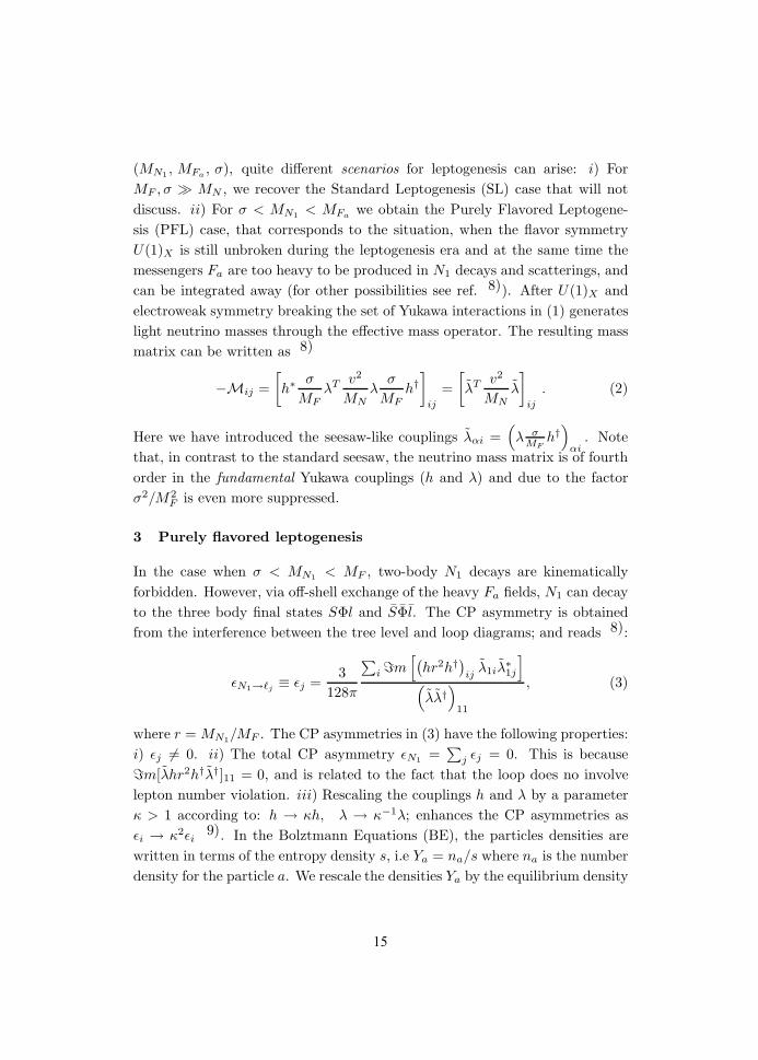
3 Purely flavored leptogenesis

In the case when σ < MN1< MF , two-body N1 decays are kinematically

forbidden. However, via off-shell exchange of the heavy Fa fields, N1 can decay

to the three body final states SΦl and SΦl. The CP asymmetry is obtained

from the interference between the tree level and loop diagrams; and reads 8):

εN1→j≡ εj =

3

128π

∑i m

[(hr2h†

)ij

λ1iλ∗

1j

](λλ†

)11

, (3)

where r = MN1/MF . The CP asymmetries in (3) have the following properties:

i) εj = 0. ii) The total CP asymmetry εN1=∑

j εj = 0. This is because

m[λhr2h†λ†]11 = 0, and is related to the fact that the loop does no involve

lepton number violation. iii) Rescaling the couplings h and λ by a parameter

κ > 1 according to: h → κh, λ → κ−1λ; enhances the CP asymmetries as

εi → κ2εi9). In the Bolztmann Equations (BE), the particles densities are

written in terms of the entropy density s, i.e Ya = na/s where na is the number

density for the particle a. We rescale the densities Ya by the equilibrium density

15

N1

S

i

Φ N1

S i

Φ N1

Φ i

S N1

i Φ

S

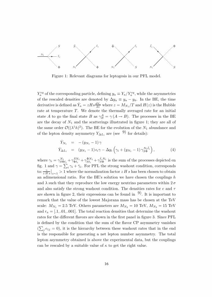
Figure 1: Relevant diagrams for leptogesis in our PFL model.

Y eqa of the corresponding particle, defining ya ≡ Ya/Y eq

a , while the asymmetries

of the rescaled densities are denoted by ∆ya ≡ ya − ya. In the BE, the time

derivative is defined as Ya = zHsdYa

dzwhere z = MN1

/T and H(z) is the Hubble

rate at temperature T . We denote the thermally averaged rate for an initial

state A to go the final state B as γAB = γ (A → B). The processes in the BE

are the decay of N1 and the scatterings illustrated in figure 1; they are all of

the same order O((λ†h)2). The BE for the evolution of the N1 abundance and

of the lepton density asymmetry Y∆Liare (see 9) for details):

YN1= − (yN1

− 1) γ

Y∆Li= (yN1

− 1) εiγ − ∆yi

(γi + (yN1

− 1) γN1i

SΦ

), (4)

where γi = γN1

SΦi+γSN1

Φi+γΦN1

Si+γ iN1

SΦ is the sum of the processes depicted en

fig. 1 and γ =∑

i γi + γi. For PFL the strong washout condition, corresponds

to: γz H s

∣∣z∼1

> 1 where the normalization factor z H s has been chosen to obtain

an adimensional ratio. For the BE’s solution we have chosen the couplings h

and λ such that they reproduce the low energy neutrino parameters within 2σ

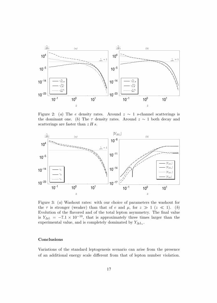
and also satisfy the strong washout condition. The densities rates for e and τ

are shown in figure 2, their expressions can be found in 9). It is important to

remark that the value of the lowest Majorana mass has be chosen at the TeV

scale: MN1= 2.5 TeV. Others parameters are MN2

= 10 TeV, MN3= 15 TeV

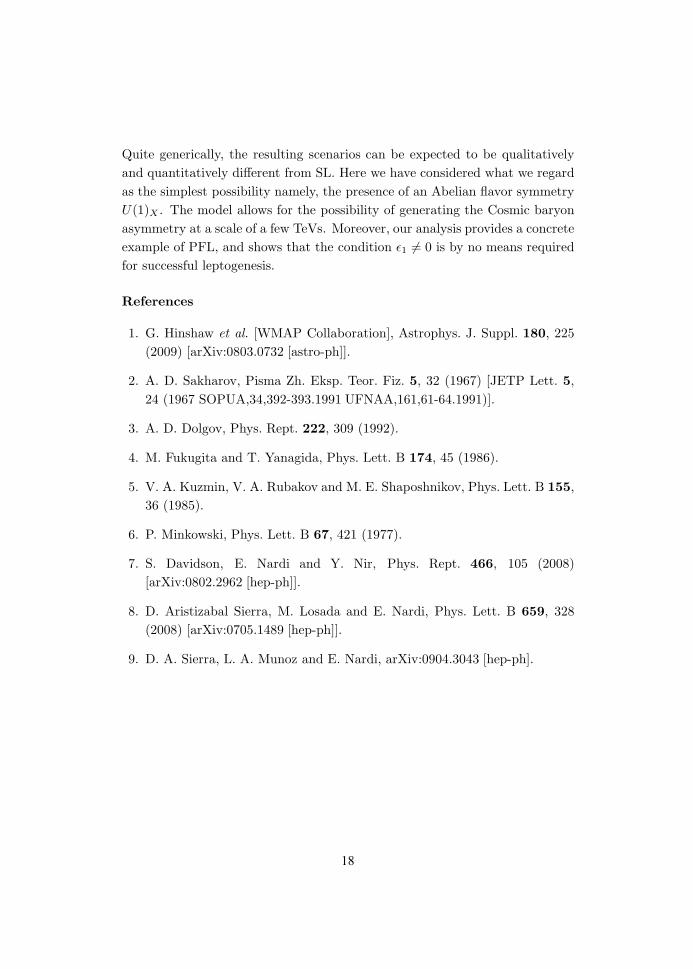
and ra = [.1, .01, .001]. The total reaction densities that determine the washout

rates for the different flavors are shown in the first panel in figure 3. Since PFL

is defined by the condition that the sum of the flavor CP asymmetry vanishes

(∑

j ε1j = 0), it is the hierarchy between these washout rates that in the end

is the responsible for generating a net lepton number asymmetry. The total

lepton asymmetry obtained is above the experimental data, but the couplings

can be rescaled by a suitable value of κ to get the right value.

16

100 101101

104

105

1014

1023

γzHs

z

γN1

SeΦ

γSN1

eΦ

γ eN1

ΦS

γ

zHs= 1

(a)

100 101101

104

105

1014

1023

γzHs

z

γN1

SτΦ

γSN1

τΦ

γ τ N1

ΦS

γ

zHs= 1

(b)

Figure 2: (a) The e density rates. Around z ∼ 1 s-channel scatterings isthe dominant one. (b) The τ density rates. Around z ∼ 1 both decay andscatterings are faster than z H s.

100 101101

104

105

1014

1023

γzHs

z

γe

γµ

γτ

γ

zHs= 1

(a)

100 101101

108

1011

1014

1017

|Y∆Li|

z

|Y∆Le|

|Y∆Lµ|

|Y∆Lτ|

|Y∆L|

(b)

Figure 3: (a) Washout rates: with our choice of parameters the washout forthe τ is stronger (weaker) than that of e and µ, for z 1 (z 1). (b)Evolution of the flavored and of the total lepton asymmetry. The final valueis Y∆L = −7.1 × 10−10, that is approximately three times larger than theexperimental value, and is completely dominated by Y∆Le

.

Conclusions

Variations of the standard leptogenesis scenario can arise from the presence

of an additional energy scale different from that of lepton number violation.

17

Quite generically, the resulting scenarios can be expected to be qualitatively

and quantitatively different from SL. Here we have considered what we regard

as the simplest possibility namely, the presence of an Abelian flavor symmetry

U(1)X . The model allows for the possibility of generating the Cosmic baryon

asymmetry at a scale of a few TeVs. Moreover, our analysis provides a concrete

example of PFL, and shows that the condition ε1 = 0 is by no means required

for successful leptogenesis.

References

1. G. Hinshaw et al. [WMAP Collaboration], Astrophys. J. Suppl. 180, 225

(2009) [arXiv:0803.0732 [astro-ph]].

2. A. D. Sakharov, Pisma Zh. Eksp. Teor. Fiz. 5, 32 (1967) [JETP Lett. 5,

24 (1967 SOPUA,34,392-393.1991 UFNAA,161,61-64.1991)].

3. A. D. Dolgov, Phys. Rept. 222, 309 (1992).

4. M. Fukugita and T. Yanagida, Phys. Lett. B 174, 45 (1986).

5. V. A. Kuzmin, V. A. Rubakov and M. E. Shaposhnikov, Phys. Lett. B 155,

36 (1985).

6. P. Minkowski, Phys. Lett. B 67, 421 (1977).

7. S. Davidson, E. Nardi and Y. Nir, Phys. Rept. 466, 105 (2008)

[arXiv:0802.2962 [hep-ph]].

8. D. Aristizabal Sierra, M. Losada and E. Nardi, Phys. Lett. B 659, 328

(2008) [arXiv:0705.1489 [hep-ph]].

9. D. A. Sierra, L. A. Munoz and E. Nardi, arXiv:0904.3043 [hep-ph].

18

Frascati Physics Series Vol. XLVIII (2009), pp. 19-24Young Researchers Workshop: “Physics Challenges in the LHC Era”

Frascati, May 11 and 14, 2009

HADRONIC τ DECAYS INTO TWO AND THREE MESONMODES WITHIN RESONANCE CHIRAL THEORY

Pablo RoigIFIC (CSIC-Universitat de Valencia) and Physik Department (TUM-Munchen)

Abstract

We study two and three meson decays of the tau lepton within the frameworkof the Resonance Chiral Theory, that is based on the following properties ofQCD: its chiral symmetry in the massless case, its large-NC limit, and theasymptotic behaviour it demands to the relevant form factors.Most of the couplings in the Lagrangian are determined this way rendering thetheory predictive. Our outcomes can be tested thanks to the combination of avery good experimental effort (current and forthcoming, at B- and tau-charm-factories) and the very accurate devoted Monte Carlo generators.

1 Hadronic decays of the τ lepton

Our purpose is to provide a description of the semileptonic decays of the tau

lepton that incorporates as many theoretical restrictions derived from the fun-

damental interaction, QCD 1), as possible. This is a very convenient scenario

19

to investigate the hadronization of QCD because one fermionic current is purely

leptonic and thus calculable unambiguously so that we can concentrate our ef-

forts on the other one, involving light quarks coupled to a V − A current.

The decay amplitude for the considered decays may be written as:

M = −GF√2

Vud/us uντγµ(1 − γ5)uτHµ , (1)

where the strong interacting part is encoded in the hadronic vector, Hµ:

Hµ = 〈 P (pi)n

i=1 | (Vµ −Aµ) eiLQCD |0 〉 . (2)

Symmetries let us decompose Hµ depending on the number of final-state pseu-

doscalar (P ) mesons, n.

One meson tau decays can be predicted in terms of the measured processes

(π/K)− → µ−νµ, since the matrix elements are related. This provides a pre-

cise test of charged current universality 2). On the other side, it cannot tell

anything new on hadronization.

The two-pion tau decay is conventionally parameterized -in the isospin limit,

that we always assume- just in terms of the vector (JP = 1−) form factor of

the pion, Fπ(s):

〈π−π0|dγµu|0 〉 ≡ 〈π−π0|V µeiLQCD |0 〉 ≡√

2Fπ(s)(pπ− − pπ0)µ , (3)

where s ≡ (pπ− + pπ0)2.

Because SU(3) is broken appreciably by the difference between ms and (mu +

md)/2, two form factors are needed to describe the decays involving one pion

and one kaon:

〈π−(p′)K0(p)|V µeiLQCD |0 〉 ≡(

QµQν

Q2− gµν

)(p − p′)νFKπ

+ (Q2)

− m2K − m2

π

Q2QµFKπ

0 (Q2) , (4)

where Qµ ≡ (p + p′)µ. FKπ+ (Q2) carries quantum numbers 1−, while FKπ

0 (Q2)

is the pseudoscalar form factor (0−). Other two meson decays can be treated

similarly and one should take advantage of the fact that chiral symmetry relates

some of their matrix elements.

For three mesons in the final state, the most general decomposition reads:

Hµ = V1µFA1 (Q2, s1, s2) + V2µFA

2 (Q2, s1, s2) +

QµFA3 (Q2, s1, s2) + i V3µFV

4 (Q2, s1, s2) , (5)

20

and

V1µ =

(gµν − QµQν

Q2

)(p2 − p1)

ν , V2µ =

(gµν − QµQν

Q2

)(p3 − p1)

ν ,

V3µ = εµνσ pν1 p

2 pσ3 , Qµ = (p1 + p2 + p3)µ , si = (Q − pi)

2 . (6)

Fi, i = 1, 2, 3, correspond to the axial-vector current (Aµ) while F4 drives the

vector current (Vµ). The form factors F1 and F2 have a transverse structure

in the total hadron momenta, Qµ, and drive a JP = 1+ transition. The

pseudoscalar form factor, F3, vanishes as m2P /Q2 and, accordingly, gives a tiny

contribution. Higher-multiplicity modes can be described proceeding similarly3). This is as far as we can go without model assumptions, that is, it is not

yet known how to obtain the Fi from QCD. However, one can derive some of

their properties from the underlying theory, as we will explain in the following.

2 Theoretical framework: Resonance Chiral Theory

We use a phenomenological Lagrangian 4) written in terms of the relevant

degrees of freedom that become active through the energy interval spanned by

hadronic tau decays. The chiral symmetry of massless QCD determines 5)

the chiral invariant operators that can be written including the lightest mesons

in the spectrum, the pseudoscalar ones belonging to the pion multiplet. It was

carefully checked 6) that -as one expects- Chiral Perturbation Theory, χPT ,

can only describe a little very-low-energy part of semileptonic tau decays.

Then one may attempt to extend the range of applicability of χPT to higher

energies while keeping its predictions for the form factors at low momentum:

this is the purpose of Resonance Chiral Theory, RχT , 7) that includes the

light-flavoured resonances as explicit fields in the action.

At LO in the NC → ∞ limit of QCD 8) one has as infinite tower of stable

mesons that experience local effective interactions at tree level. We depart from

this picture in two ways:

• We incorporate the widths of the resonances worked out consistently

within RχT 9).

• We attempt a description including the least possible number of resonance

fields reducing -ideally- to the single resonance approximation, SRA 10).

21

We take vector meson dominance into account when writing our Lagrangian.

Thus, it will consist of terms accounting for the following interactions (aµ,

vµ stand for the axial(-vector) currents and A and V for the axial(-vector)

resonances):

• Those in χPT at LO and χPT -like: aµP , aµPPP , PPPP with even-

intrinsic parity; and vµPPP in the odd-intrinsic parity sector.

• Those relevant in RχT -NLO χPT operators are not included to avoid

double counting, since they are recovered and their couplings are satu-

rated upon integration of the resonance contributions 7)-. They include:

aµV P , vµV , aµA, V PP and AV P in the even-intrinsic parity sector and

vµV P , V PPP and V V P in the odd-parity one.

The explicit form of the operators and the naming for the couplings can be

read from 7), 11), 12), 13), 14) and 15).

The RχT just determined by symmetries does not share the UV QCD be-

haviour yet. For this, and for our purposes, we need to impose appropriate

Brodsky-Lepage conditions 16) on the relevant form factors. Explicit com-

putation and these short-distance restrictions reduce appreciably the number

of independent couplings entering the amplitudes which enables us to end up

with a useful -that is, predictive- theory.

3 Phenomenology

Our framework describes pretty well the two-meson decays of the τ , as shown

in the ππ 17) and Kπ 18) cases. Two-meson modes including η can be

worked analogously. The data in these modes are so precise 1 that although

the SRA describes the gross features of the data, one needs to include the first

excitations of the V resonances to achieve an accurate description. Although

FKπ+ (Q2) is much more important than FKπ

0 (Q2), one needs an appropriate

pseudoscalar form factor to fit well the data, specially close to threshold 18).

The three meson modes are much more involved. However, a good descrip-

tion of the data has been achieved through a careful study 12, 15) taking

into account all theory constrains and experimental data on the 3π and KKπ

channels. We predict the KKπ spectral function and conclude that the vector

1See the references quoted in the articles cited through the section.

22

current contribution cannot be neglected in these modes. We will study the

other three meson modes along the same lines. In particular, our study of the

Kππ channels might help improve the simultaneous extraction of ms and Vus

19). Our expressions for the vector and axial-vector widths and the hadronic

matrix elements have been implemented successfully in the TAUOLA library20). This way, the experimental comunity will have as its disposal a way of

analysing hadronic decays of the tau that includes as much as possible infor-

mation from the fundamental theory. We also plan to study e+e− → PPP at

low energies what can eventually be used by 21).

4 Acknowledgements

I congratulate the local organizing committee for this first edition of the Young

Researchers Workshop as well as for the XIV LNF SPRING SCHOOL BRUNO

TOUSCHEK held in parallel. I am grateful to Jorge Portoles for a careful

revision and useful suggestions on the draft. I acknowledge useful discussions

with Olga Shekhovtsova. This work has been supported in part by the EU

MRTN-CT-2006-035482 (FLAVIAnet) and by the DFG cluster of excellence

’Origin and structure of the Universe’ .

References

1. H. Fritzsch, M. Gell-Mann and H. Leutwyler, Phys. Lett. B 47 (1973) 365.

D. J. Gross and F. Wilczek, Phys. Rev. Lett. 30 (1973) 1343. H. D. Politzer,

Phys. Rev. Lett. 30 (1973) 1346.

2. A. Pich, Nucl. Phys. Proc. Suppl. 98 (2001) 385. Nucl. Phys. Proc. Suppl.

181-182 (2008) 300.

3. R. Fischer, J. Wess and F. Wagner, Z. Phys. C 3 (1979) 313.

4. S. Weinberg, Physica A 96 (1979) 327.

5. J. Gasser and H. Leutwyler, Annals Phys. 158 (1984) 142. Nucl. Phys. B

250 (1985) 465.

6. G. Colangelo, M. Finkemeier and R. Urech, Phys. Rev. D 54 (1996) 4403.

23

7. G. Ecker, J. Gasser, A. Pich and E. de Rafael, Nucl. Phys. B 321 (1989)

311. G. Ecker, J. Gasser, H. Leutwyler, A. Pich and E. de Rafael, Phys.

Lett. B 223 (1989) 425.

8. G. ’t Hooft, Nucl. Phys. B 72 (1974) 461, 75 (1974) 461. E. Witten, Nucl.

Phys. B 160 (1979) 57.

9. D. Gomez Dumm, A. Pich and J. Portoles, Phys. Rev. D 62 (2000) 054014.

10. M. Knecht, S. Peris, M. Perrottet and E. de Rafael, Phys. Rev. Lett. 83

(1999) 5230.

11. P. D. Ruiz-Femenıa, A. Pich and J. Portoles, JHEP 0307 (2003) 003.

12. D. Gomez Dumm, A. Pich and J. Portoles, Phys. Rev. D 69 (2004) 073002.

13. V. Cirigliano, G. Ecker, M. Eidemuller, A. Pich and J. Portoles, Phys. Lett.

B 596 (2004) 96.

14. P. Roig, AIP Conf. Proc. 964 (2007) 40.

15. D. Gomez-Dumm, P. Roig, A. Pich, J. Portoles, to appear.

16. S. J. Brodsky and G. R. Farrar, Phys. Rev. Lett. 31 (1973) 1153. G. P. Lep-

age and S. J. Brodsky, Phys. Rev. D 22 (1980) 2157.

17. F. Guerrero and A. Pich, Phys. Lett. B 412 (1997) 382. A. Pich and J. Por-

toles, Phys. Rev. D 63 (2001) 093005. Nucl. Phys. Proc. Suppl. 121 (2003)

179.

18. M. Jamin, A. Pich and J. Portoles, Phys. Lett. B 640 (2006) 176 Phys.

Lett. B 664 (2008) 78.

19. E. Gamiz, M. Jamin, A. Pich, J. Prades and F. Schwab, Phys. Rev. Lett.

94 (2005) 011803.

20. O.Shekhovtsova, private communication.

21. G. Rodrigo, H. Czyz, J. H. Kuhn and M. Szopa, Eur. Phys. J. C 24 (2002)

71.

24

Frascati Physics Series Vol. XLVIII (2009), pp. 25-30Young Researchers Workshop: “Physics Challenges in the LHC Era”

Frascati, May 11 and 14, 2009

MEASUREMENT OF THE MISSING TRANSVERSE ENERGYIN THE ATLAS DETECTOR

Giovanni SiragusaJohannes Gutenberg Universitat - Mainz (DE)

Abstract

A very good measurement of the Missing Transverse Energy (EmissT ) is a crucial

requirement for the study of many physics processes at the LHC, for examplethe Standard Model W or top-quark production, Higgs bosons decaying to taupairs, or supersymmetric particles. The most important contribution to theEmiss

T resolution in the ATLAS detector comes from the calorimeters, whichprovide near hermetic energy reconstruction. The calorimeter noise suppressionis of crucial importance and can be achieved using either a simple noise cutor more sophisticated topological criteria. A refined calibration improves theEmiss

T measurement. Additional corrections are applied for muons detected inthe Muon Spectrometer and energy deposits in dead material, as the cryostatof the calorimeter. A detailed study of the Missing Energy performance onfully simulated Monte Carlo data is presented, which shows results for variousphysics processes involving different level of hadronic activity and Emiss

T . RealATLAS data from cosmic runs are also compared with the results from thedetector simulation.

25

1 Introduction

At Tevatron and at the Large Hadron Collider (LHC) events with large Trans-

verse Missing Energy (EmissT ) are expected to be key signatures of new physics

(SUSY, Extra Dimensions). A good measurement of EmissT in terms of linearity

and resolution is important for the reconstruction of the top-quark mass and

for the study of W bosons decays. A precise EmissT measurement is also crucial

for the efficient and accurate reconstruction of the Higgs boson mass, when

decaying to a pair of τ leptons.

At hadron colliders it is not possible to use the Centre of Mass Energy to

constrain the kinematic of observed decays, but only the conservation of the

longitudinal momentum. To reconstruct the transverse momentum (pT ) of non

interacting particles we make use of the conservation of the total longitudinal

momentum of the event:−→ET

miss= −−→

ET

visible. For this reason the LHC gen-

eral purpose detectors have been designed with calorimeters covering a large

solid angle. In particular, the ATLAS calorimeter is able to provide a precise

energy measurement up to a pseudo-rapidity of |η| < 4.9.

To properly reconstruct the visible energy of the event, each energy deposit

has to be calibrated accordingly to the associated physics process. One of

the challenges of the measurement is to calibrate the energy deposited by soft

interactions, which contribute significantly to the total visible energy of the

event. The main sources of soft deposits are inelastic proton-proton collisions

(pile-up) and the underlying event. The limited coverage of the ATLAS Inner

Detector and of the Muon Spectrometer, and the cracks of the Calorimeters in

the barrel-endcap transition region affect the EmissT measurement.

2 EmissT reconstruction

To measure EmissT in ATLAS two approaches are used: the first (that we will

denote as cell-based reconstruction) starts from the calorimeter cells and adds

calibration and corrections in further steps, the second (that we will denote

as object-based reconstruction) starts from identified objects and adds the con-

tribution from soft deposits in a second step. The cell-based reconstruction is

more robust at initial data-taking, and less dependent on the definition of each

single physics object. The object based reconstruction, on the other side, has

the advantage to treat separately low-energy deposits: isolated clusters are col-

26

lected in the so called mini jets, then π± and π0 are identified and calibrated.

Given the high number of electronic channels in the calorimeters (∼ 200 k), an

efficient noise suppression is required to improve the resolution. The easiest ap-

proach consists in a determination of the electronic noise, which is then used to

apply a cut on each calorimeter cell energy, usually requiring Ecell > 2 × σnoise.

A more effective approach, while less conservative, is the Topological Cluster-

ing, with the search for three-dimensional clusters of cells. Starting from a

cluster seed (a cell with an energy above 4 × σnoise), all the neighbouring

cells with energy above 2 × σnoise are added to the cluster, then all their

neighbouring cells without requiring any energy cut. With this method cells

with very low signal can survive the noise cut because of a signal measured in a

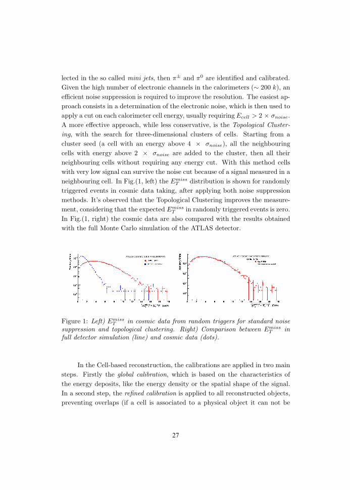
neighbouring cell. In Fig.(1, left) the EmissT distribution is shown for randomly

triggered events in cosmic data taking, after applying both noise suppression

methods. It’s observed that the Topological Clustering improves the measure-

ment, considering that the expected EmissT in randomly triggered events is zero.

In Fig.(1, right) the cosmic data are also compared with the results obtained

with the full Monte Carlo simulation of the ATLAS detector.

Figure 1: Left) EmissT in cosmic data from random triggers for standard noise

suppression and topological clustering. Right) Comparison between EmissT in

full detector simulation (line) and cosmic data (dots).

In the Cell-based reconstruction, the calibrations are applied in two main

steps. Firstly the global calibration, which is based on the characteristics of

the energy deposits, like the energy density or the spatial shape of the signal.

In a second step, the refined calibration is applied to all reconstructed objects,

preventing overlaps (if a cell is associated to a physical object it can not be

27

associated to another one). The Object-based reconstruction, on the other

hand, starts from calibrated objects and then performs a further calibration of

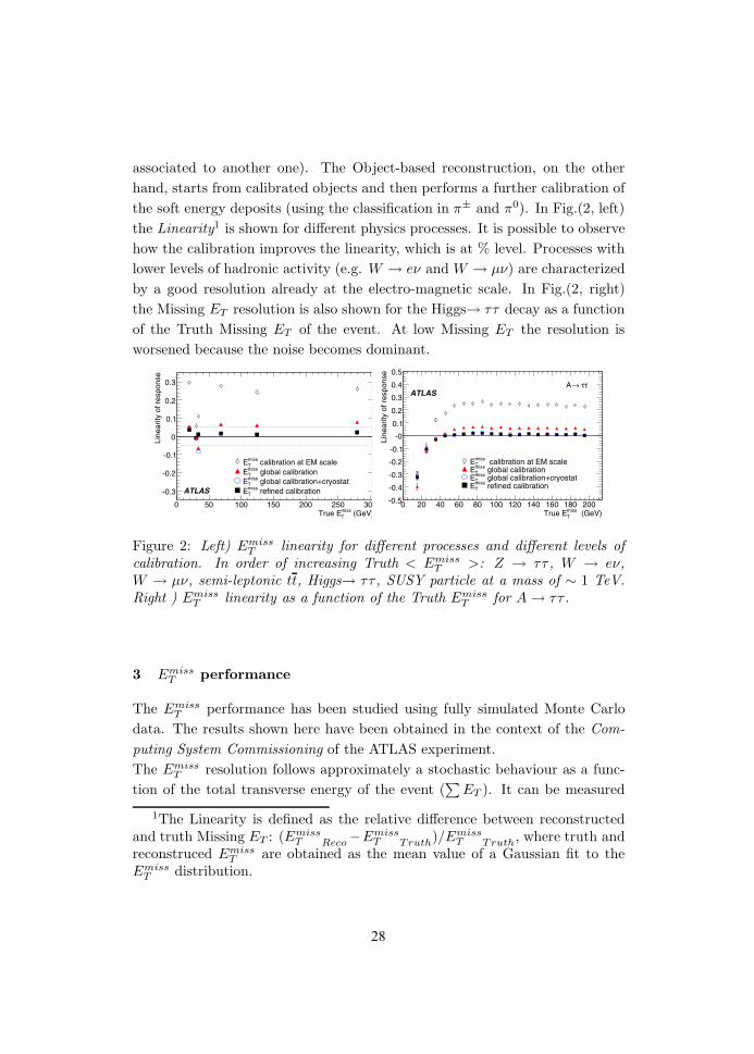
the soft energy deposits (using the classification in π± and π0). In Fig.(2, left)

the Linearity1 is shown for different physics processes. It is possible to observe

how the calibration improves the linearity, which is at % level. Processes with

lower levels of hadronic activity (e.g. W → eν and W → µν) are characterized

by a good resolution already at the electro-magnetic scale. In Fig.(2, right)

the Missing ET resolution is also shown for the Higgs→ ττ decay as a function

of the Truth Missing ET of the event. At low Missing ET the resolution is

worsened because the noise becomes dominant.

(GeV)missTTrue E

0 50 100 150 200 250 300

Line

arity

of r

espo

nse

-0.3

-0.2

-0.1

0

0.1

0.2

0.3

global calibration+cryostatmissTE

refined calibrationmissTE

calibration at EM scalemissTE

global calibrationmissTE

ATLAS

(GeV)missTTrue E

0 20 40 60 80 100 120 140 160 180 200

Line

arity

of r

espo

nse

-0.5

-0.4

-0.3

-0.2

-0.1

-0

0.1

0.2

0.3

0.4

0.5

refined calibrationmissTE

ττ→A

calibration at EM scalemissTE

global calibrationmissTE

global calibration+cryostatmissTE

ATLAS

Figure 2: Left) EmissT linearity for different processes and different levels of

calibration. In order of increasing Truth < EmissT >: Z → ττ , W → eν,

W → µν, semi-leptonic tt, Higgs→ ττ , SUSY particle at a mass of ∼ 1 TeV.

Right ) EmissT linearity as a function of the Truth Emiss

T for A → ττ .

3 EmissT performance

The EmissT performance has been studied using fully simulated Monte Carlo

data. The results shown here have been obtained in the context of the Com-

puting System Commissioning of the ATLAS experiment.

The EmissT resolution follows approximately a stochastic behaviour as a func-

tion of the total transverse energy of the event (∑

ET ). It can be measured

1The Linearity is defined as the relative difference between reconstructedand truth Missing ET : (Emiss

T Reco−Emiss

T Truth)/Emiss

T Truth, where truth and

reconstruced EmissT are obtained as the mean value of a Gaussian fit to the

EmissT distribution.

28

in-situ using known processes with zero expected EmissT , like minimum bias

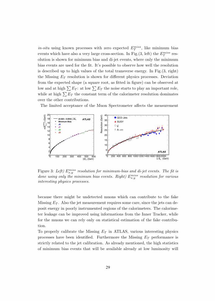
events which have also a very large cross-section. In Fig.(3, left) the EmissT res-

olution is shown for minimum bias and di-jet events, where only the minimum

bias events are used for the fit. It’s possible to observe how well the resolution

is described up to high values of the total transverse energy. In Fig.(3, right)

the Missing ET resolution is shown for different physics processes. Deviation

from the expected shape (a square root, as fitted in figure) can be observed at

low and at high∑

ET : at low∑

ET the noise starts to play an important role,

while at high∑

ET the constant term of the calorimeter resolution dominates

over the other contributions.

The limited acceptance of the Muon Spectrometer affects the measurement

(GeV)TEΣ0 100 200 300 400 500 600

) (G

eV)

mis

s

X,Y

(Eσ

0

2

4

6

8

10

12

14

16

18

20

TEΣ 0.003) ±(0.520Minimum BiasJ0J1J2J3

ATLAS

(GeV)T EΣ0 200 400 600 800 1000 120014001600 18002000

Res

olut

ion

(GeV

)

0

5

10

15

20

25

30

35

40

SUSY

QCD Jets

tt

ττ→A

ATLAS

Figure 3: Left) Emissx,y resolution for minimum-bias and di-jet events. The fit is

done using only the minimum bias events. Right) Emissx,y resolution for various

interesting physics processes.

because there might be undetected muons which can contribute to the fake

Missing ET . Also the jet measurement requires some care, since the jets can de-

posit energy in poorly instrumented regions of the calorimeters. The calorime-

ter leakage can be improved using informations from the Inner Tracker, while

for the muons we can rely only on statistical estimation of the fake contribu-

tion.

To properly calibrate the Missing ET in ATLAS, various interesting physics

processes have been identified. Furthermore the Missing ET performance is

strictly related to the jet calibration. As already mentioned, the high statistics

of minimum bias events that will be available already at low luminosity will

29

be very useful for understanding the QCD environment at the LHC energies.

Di-jet events are as much powerful as minimum bias and, despite that of a

lower statistics, they present higher values of∑

ET . Other processes that are

useful for the understanding of the Missing ET are Z → e+e− and Z → µ+µ−,

which acn give interesting results in terms of resolution and acceptance, while

Z → τ+τ− can be used to fix the EmissT scale.

4 Conclusion

The main aspects of the Missing ET reconstruction and performance in ATLAS

have been shown. Detailed MC studies demonstrate that the expected perfor-

mance can be achieved, while runs with random triggers have demonstrated

that the description and suppression of the instrumental noise work well. In

view of first collision data, further studies of the cosmic data will improve our

understanding of the Missing ET .

References

1. The ATLAS Collaboration, ”Expected performance of the ATLAS Exper-

iment: Detector, Trigger and Physics”, arXiv:0901.0512; CERN-OPEN-

2008-20 (December 2008).

30

Frascati Physics Series Vol. XLVIII (2009), pp. 31-36Young Researchers Workshop: “Physics Challenges in the LHC Era”

Frascati, May 11 and 14, 2009

MEASUREMENT OF THE pp→ Z→ µµ + X CROSS SECTIONAT LHC WITH ATLAS EXPERIMENT

Roberto Di NardoINFN & University of Rome “Tor Vergata”

Via della Ricerca Scientifica 1, 00133 Rome

Abstract

One of the first Standard Model processes that can be studied with the ATLASdetector at the Large Hadron Collider will be the Z boson production in protonproton collisions. Due to its high production rate, the differents decay channelsof the Z boson will also be used in the initial data taking period as benchmarkprocesses for the calibration of the detectors and performance measurements.The measurement of the cross section of pp→Z→ µ+µ− + X process with firstdata in ATLAS experiment is discussed.

1 Introduction

Due to large production rates, the physics of W and Z bosons is accessible in

the early data taking phase of the ATLAS 1) experiment at the LHC and will

be used as standard candle for many measurements. Depending on integrated

31

luminosity, their leptonic decay channels can be used for the commissioning of

detectors and debugging of the analysis tools or the precision measurement of

electroweak parameters.

The production cross section of the Z boson can be written as

σZ =N − B

A × ε × ∫ Ldt(1)

where N is the number of selected candidate events, B is the number of back-

ground events, A is the detector acceptance computed from MC studies, L is

the luminosity and ε includes the reconstruction and trigger efficiency and the

signal selection cut efficiency.

The measurement uncertainty gets contribution from different terms as follows

δσ

σ=

δN ⊕ δB

N − B⊕ δL

L⊕ δA

A⊕ δε

ε(2)

The term δN has a pure statistic origin and the relative error will decrease with

increasing integrated luminosity L , following the relation δN/N ∼ 1/√

L .

The other terms are δB due to background contribution, δA that reflects the

theoretical uncertainties on the acceptance and δε that is related to the lim-

ited detector response knowledge. All of these are systematic uncertainties

in the cross section measurement but they can be constrained with auxiliary

measurements. An overall luminosity uncertainty of δL /L = 10% should be

taken into account for the measurement with the first ∼ 50pb−1 of integrated

luminosity, but it is expected to decrease in time thanks to the better under-

standing of the LHC beam parameters and of the ATLAS luminosity detector

response.

In the following sections, the measurement of σ (pp → Z) × BR (Z → µµ) is

discussed. Section 2 will focus on the event selection while in the other chapter

the techniques for the determination of the detector performance from data are

shortly described: the muon momentum scale and resolution (section 3) and

the measurement of muon reconstruction and trigger efficiency (section 4).

2 Event Selection

The Z → µ+µ− signal selection begins requiring at least a muon track candi-

date that passes the 10 GeV single muon trigger. Events are further selected

by requiring that they contain at least two reconstructed muon tracks with a

32

ID Tracks0.05<r<0.5N

0 2 4 6 8 10 12 14 16 18

Arb

itrar

y un

its

ATLASµµ→Zνµ→Wµµ→bb

µµ→tt

ττ→Z

(a)

[GeV]µµm40 50 60 70 80 90 100 110 120

Num

ber

of E

vent

s/G

eV

500

1000

1500

2000

2500

3000

3500

4000ATLAS µµ→Z

νµ→Wµµ→bb

µµ→ttττ→Z

(b)

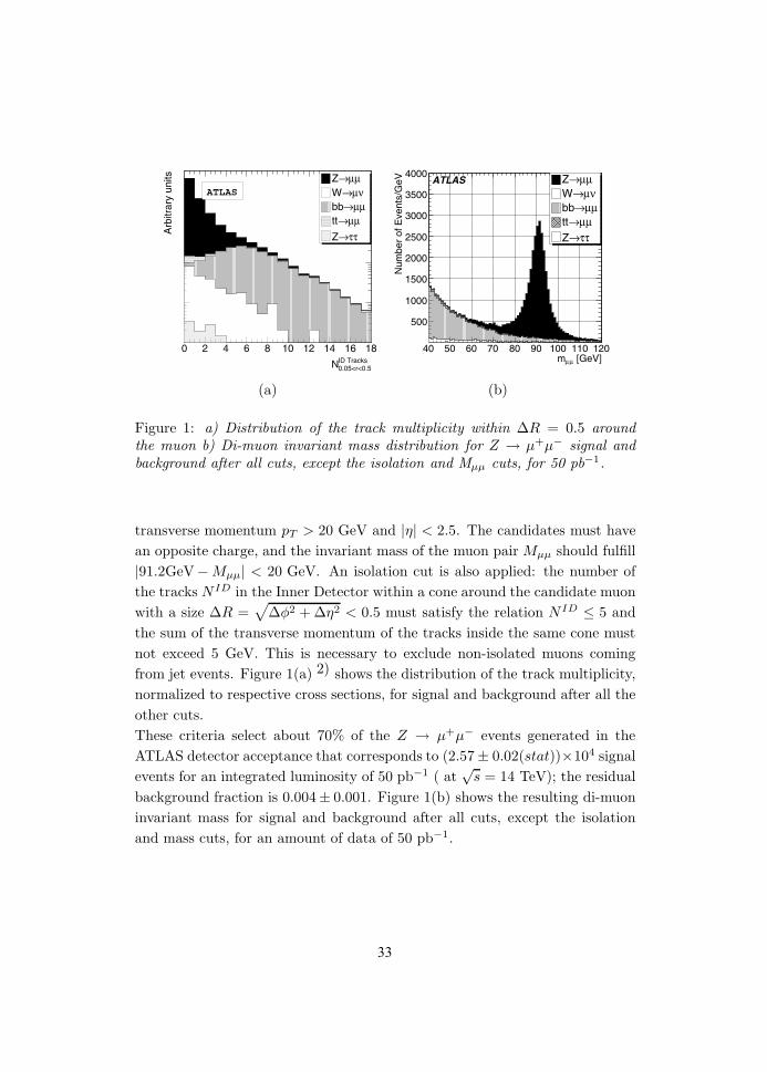
Figure 1: a) Distribution of the track multiplicity within ∆R = 0.5 around

the muon b) Di-muon invariant mass distribution for Z → µ+µ− signal and

background after all cuts, except the isolation and Mµµ cuts, for 50 pb−1.

transverse momentum pT > 20 GeV and |η| < 2.5. The candidates must have

an opposite charge, and the invariant mass of the muon pair Mµµ should fulfill

|91.2GeV− Mµµ| < 20 GeV. An isolation cut is also applied: the number of

the tracks N ID in the Inner Detector within a cone around the candidate muon

with a size ∆R =√

∆φ2 + ∆η2 < 0.5 must satisfy the relation N ID ≤ 5 and

the sum of the transverse momentum of the tracks inside the same cone must

not exceed 5 GeV. This is necessary to exclude non-isolated muons coming

from jet events. Figure 1(a) 2) shows the distribution of the track multiplicity,

normalized to respective cross sections, for signal and background after all the

other cuts.

These criteria select about 70% of the Z → µ+µ− events generated in the

ATLAS detector acceptance that corresponds to (2.57 ± 0.02(stat))×104 signal

events for an integrated luminosity of 50 pb−1 ( at√

s = 14 TeV); the residual

background fraction is 0.004± 0.001. Figure 1(b) shows the resulting di-muon

invariant mass for signal and background after all cuts, except the isolation

and mass cuts, for an amount of data of 50 pb−1.

33

3 Muon Momentum Scale and Resolution

The measurement of the muon momentum with the ATLAS experiment can be

affected by the limited knowledge of the magnetic field, the uncertainty in the

energy loss of the muons, and the alignment of the muon spectrometer.

The determination of the pT scale and resolution one can be made studying the

Z resonance shape. In fact the pT scale has a direct impact on the measured

mean value, while the pT resolution has a direct impact on the measured Z

width.

To extract the value of muon resolution and momentum scale, the pT resolution

function predicted by Monte Carlo simulations is iteratively adjusted in its

width and scale and the corresponding Z boson mass distribution is calculated.

The procedure stops if the resulting distribution agrees within its statistical

error to the distribution measured from data.

It is expected to determine the momentum scale for muons with a precision

better than 1%, while the uncertainty on the resolution will be smaller than

10%, for an integrated luminosity of 50 pb−1.

4 Muon Trigger and Reconstruction Efficiency

One of the methods chosen by the ATLAS experiment to evaluate the trigger

and reconstruction efficiency for muons is the so called tag and probe. This is

a data driven method which uses the two ATLAS independent traking systems

(Muon Spectrometer and Inner Detector) to cross-check their performances.

The tag and probe method is based on the definition of a probe object that is

used to make the performance measurement over a certain sample of events

properly chosen (tagged). For the efficiency studies the probe assumes the

same role of a MC truth generated muon in simulted data. In particular, the

Z → µ+µ− decay provides two muons with an high pT that can give two tracks

in the Muon Spectrometer and in the Inner Detector and two combined objects.

To apply this method in the Z → µ+µ− decay, two reconstructed tracks in the

Inner detector are required together with at least one associated track in the

muon spectrometer. The invariant mass of the two Inner Detector tracks have

to be close to the mass of the Z boson, to ensure that the tracks are the ones

associated to the decay muons of the Z boson.

In order to get as close as possible to a zero-background sample (where this

34

of the two tracksThe invariant mass

in the MS.corresponding trackTest if there is

Z−Boson mass.should be near the

Muon Spectrometer

Inner Tracker

Probe Muon

Z−Boson

Tag Muon

(a)

η-2 -1 0 1 2

Effi

cien

cy

0.4

0.5

0.6

0.7

0.8

0.9

1

ATLAS

Muon Id: Monte Carlo truth

Muon Id: Tag & Probe

Trig: Monte Carlo truth

Trig: Tag & Probe

(b)

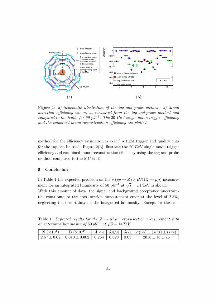
Figure 2: a) Schematic illustration of the tag and probe method. b) Muon

detection efficiency vs. η, as measured from the tag-and-probe method and

compared to the truth, for 50 pb−1. The 20 GeV single muon trigger efficiency

and the combined muon reconstruction efficiency are plotted.

method for the efficiency estimation is exact) a tight trigger and quality cuts

for the tag can be used. Figure 2(b) illustrate the 20 GeV single muon trigger

efficiency and combined muon reconstruction efficiency using the tag and probe

method compared to the MC truth.

5 Conclusion

In Table 1 the expected precision on the σ (pp → Z)×BR (Z → µµ) measure-

ment for an integrated luminosity of 50 pb−1 at√

s = 14 TeV is shown.

With this amount of data, the signal and background acceptance uncertain-

ties contribute to the cross section measurement error at the level of 2.3%,

neglecting the uncertainty on the integrated luminosity. Except for the con-

Table 1: Expected results for the Z → µ+µ− cross-section measurement with

an integrated luminosity of 50 pb−1

at√

s = 14TeV.

N (×104) B (×104) A × ε δA/A δε/ε σ(pb) ± (stat) ± (sys)2.57 ± 0.02 0.010 ± 0.002 0.254 0.023 0.03 2016± 16 ± 76

35

tribution from the acceptance, which is theoretically limited, all the others

uncertainties are expected to scale with statistics.

With the collection of a higher statistics, further studies of the differential

Z → µ+µ− cross section will also be useful to improve the theoretical un-

derstanding, thus allowing to measure the σ (pp → Z) × BR (Z → µµ) with a

precision better than 2%.

References

1. The ATLAS Collaboration, The ATLAS Experiment at the CERN Large

Hadron Collider, 2008 JINST 3 S08003

2. ATLAS Collaboration, Expected Performance of the ATLAS Experiment,

Detector, Trigger and Physics, CERN-OPEN-2008-020, Geneva, 2008.

36

Frascati Physics Series Vol. XLVIII (2009), pp. 37-42Young Researchers Workshop: “Physics Challenges in the LHC Era”

Frascati, May 11 and 14, 2009

STUDY OF THE GEOMETRICAL ACCEPTANCEFOR VECTOR BOSONS IN ATLAS

AND ITS SYSTEMATIC UNCERTAINTY

Manuela VenturiINFN and University of Roma Tor Vergata,

Via della Ricerca Scientifica 1, 00133 Rome, Italy

Abstract

The geometrical acceptance for the decays pp → W/Z + X → ν/ + − + Xin the ATLAS detector, is calculated using different Monte Carlo generators.The main contribution to its systematic error is due to Parton DistributionFunctions (PDFs).

1 Introduction

The measurement of pp → W/Z → ν/ + − cross sections will be one of the

first goals of the ATLAS experiment when the LHC will start the first collisions

in Winter 2009.

The cross section can be written as follows 1):

σ ≡ σpp→W/Z · BrW/Z→ν/+− =N − B

A · ε · L (1)

37

where Br is the branching ratio for the leptonic decays of vector bosons, N the

number of signal events, B the number of associated background events, A the

geometrical acceptance (i.e. the fraction of signal events inside the kinematical

and angular cuts), ε the efficiency inside A and L the integrated luminosity.

The geometrical acceptance is determined only by the theory: one generates

the signal and looks for the final leptons, coming from the vector boson, and

then imposes the best cuts in order to separate the signal from the background.

From eq.1 and assuming no correlation, we get the following formula to

calculate cross section uncertainty 1):

δσ

σ=

δN ⊕ δB

N − B⊕ δε

ε⊕ δL

L ⊕ δA

A(2)

where ⊕ means quadratic sum. δN/N and δB/B have a purely statistical

origin, so they will decrease as 1/√L, while δL and δε are expected to decrease

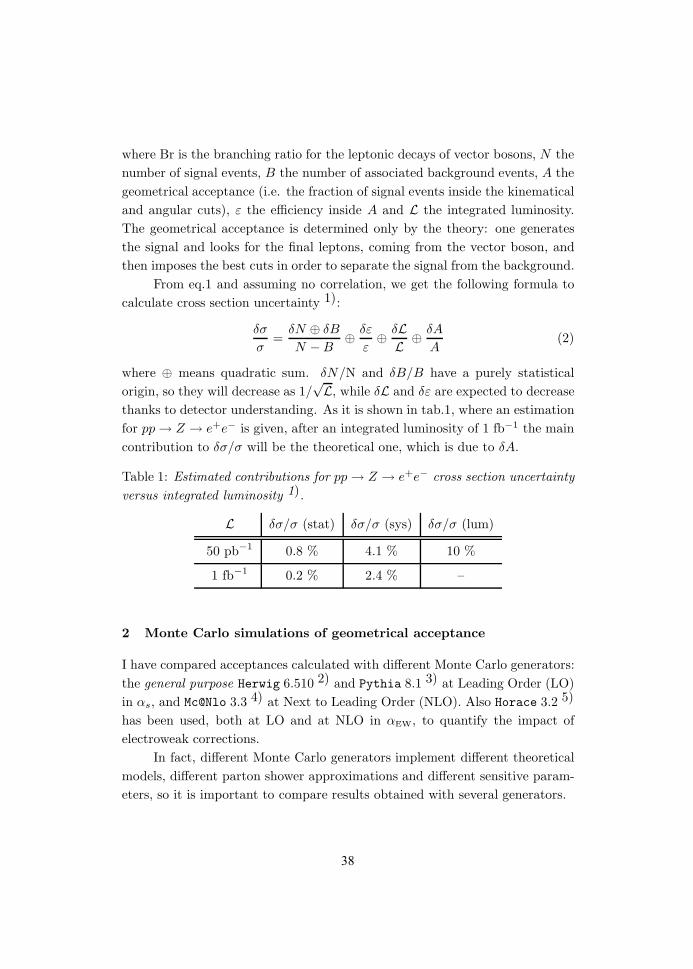
thanks to detector understanding. As it is shown in tab.1, where an estimation

for pp → Z → e+e− is given, after an integrated luminosity of 1 fb−1 the main

contribution to δσ/σ will be the theoretical one, which is due to δA.

Table 1: Estimated contributions for pp → Z → e+e− cross section uncertainty

versus integrated luminosity 1).

L δσ/σ (stat) δσ/σ (sys) δσ/σ (lum)

50 pb−1 0.8 % 4.1 % 10 %

1 fb−1 0.2 % 2.4 % –

2 Monte Carlo simulations of geometrical acceptance

I have compared acceptances calculated with different Monte Carlo generators:

the general purpose Herwig 6.510 2) and Pythia 8.1 3) at Leading Order (LO)

in αs, and Mc@Nlo 3.3 4) at Next to Leading Order (NLO). Also Horace 3.2 5)

has been used, both at LO and at NLO in αEW, to quantify the impact of

electroweak corrections.

In fact, different Monte Carlo generators implement different theoretical

models, different parton shower approximations and different sensitive param-

eters, so it is important to compare results obtained with several generators.

38

In this work, the channels = e, µ have been studied, both for W and for

Z/γ∗, at√

s = 14 TeV, in stand-alone mode and in the official ATLAS analysis

framework (Athena).

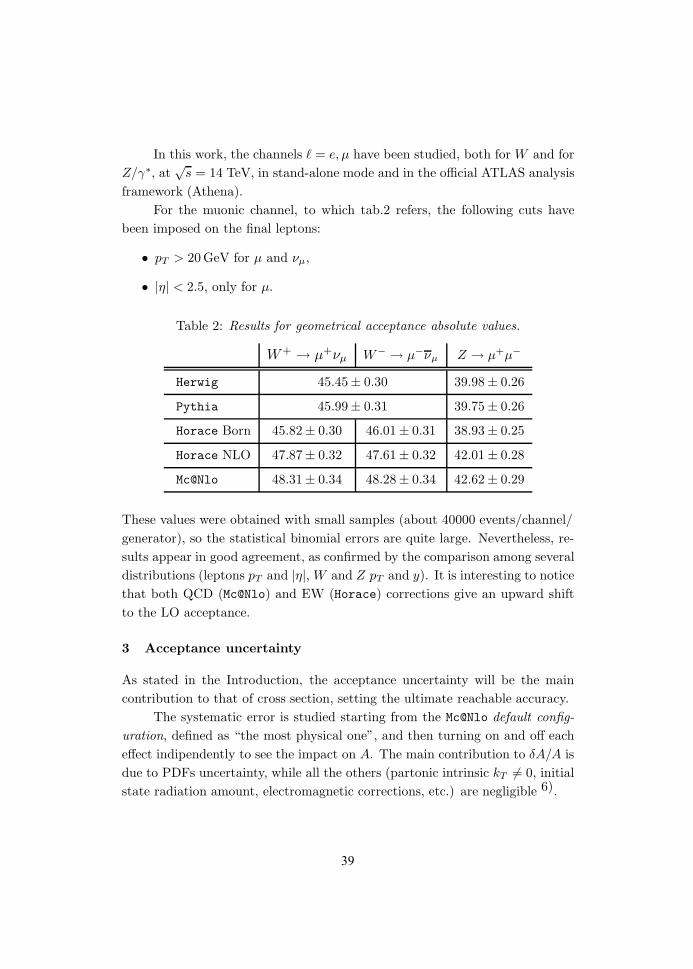
For the muonic channel, to which tab.2 refers, the following cuts have

been imposed on the final leptons:

• pT > 20 GeV for µ and νµ,

• |η| < 2.5, only for µ.

Table 2: Results for geometrical acceptance absolute values.

W+ → µ+νµ W− → µ−νµ Z → µ+µ−

Herwig 45.45± 0.30 39.98 ± 0.26

Pythia 45.99± 0.31 39.75 ± 0.26

Horace Born 45.82± 0.30 46.01± 0.31 38.93 ± 0.25

Horace NLO 47.87± 0.32 47.61± 0.32 42.01 ± 0.28

Mc@Nlo 48.31± 0.34 48.28± 0.34 42.62 ± 0.29

These values were obtained with small samples (about 40000 events/channel/

generator), so the statistical binomial errors are quite large. Nevertheless, re-

sults appear in good agreement, as confirmed by the comparison among several

distributions (leptons pT and |η|, W and Z pT and y). It is interesting to notice

that both QCD (Mc@Nlo) and EW (Horace) corrections give an upward shift

to the LO acceptance.

3 Acceptance uncertainty

As stated in the Introduction, the acceptance uncertainty will be the main

contribution to that of cross section, setting the ultimate reachable accuracy.

The systematic error is studied starting from the Mc@Nlo default config-

uration, defined as “the most physical one”, and then turning on and off each

effect indipendently to see the impact on A. The main contribution to δA/A is

due to PDFs uncertainty, while all the others (partonic intrinsic kT = 0, initial

state radiation amount, electromagnetic corrections, etc.) are negligible 6).

39

3.1 Parton Distribution Functions

Several analysis methods have been proposed to extract PDFs from data. To es-

timate δA/A, I compared the CTEQ and the Neural Network (NN) approaches.

3.1.1 CTEQ PDFs

CTEQ analysis implements the Hessian method: one chooses a priori the PDF

parametrization (NPAR = 20 free parameters for CTEQ 6.1 analysis), and then

iteratively diagonalizes the Hessian matrix, resulting in NPAR eigenvectors. The

last step requires to choose a tolerance criterion to stop the χ2global

variation

from the minimum, along each eigenvector. In this way, one ends up with

2NPAR PDF error sets plus a best fit set.

Acceptance central value, A0, is calculated with the PDF best fit set, and

then the Hessian error is associated to it through the master formula, which

takes into account the possibility of an asymmetric behaviour:

∆A+ =

√∑PAR

k=1

[max

(A+

k − A0, A−

k − A0, 0)]2

∆A− =

√∑PAR

k=1

[max

(A0 − A+

k , A0 − A−

k , 0)]2 . (3)

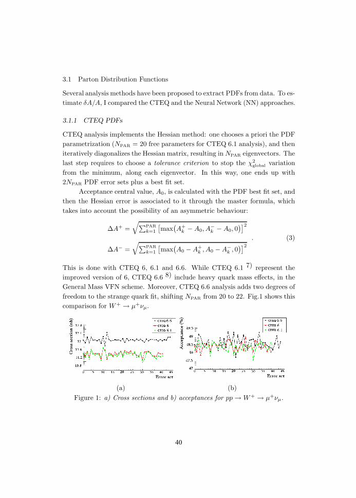
This is done with CTEQ 6, 6.1 and 6.6. While CTEQ 6.1 7) represent the

improved version of 6, CTEQ 6.6 8) include heavy quark mass effects, in the

General Mass VFN scheme. Moreover, CTEQ 6.6 analysis adds two degrees of

freedom to the strange quark fit, shifting NPAR from 20 to 22. Fig.1 shows this

comparison for W+ → µ+νµ.

(a) (b)

Figure 1: a) Cross sections and b) acceptances for pp → W+ → µ+νµ.

40

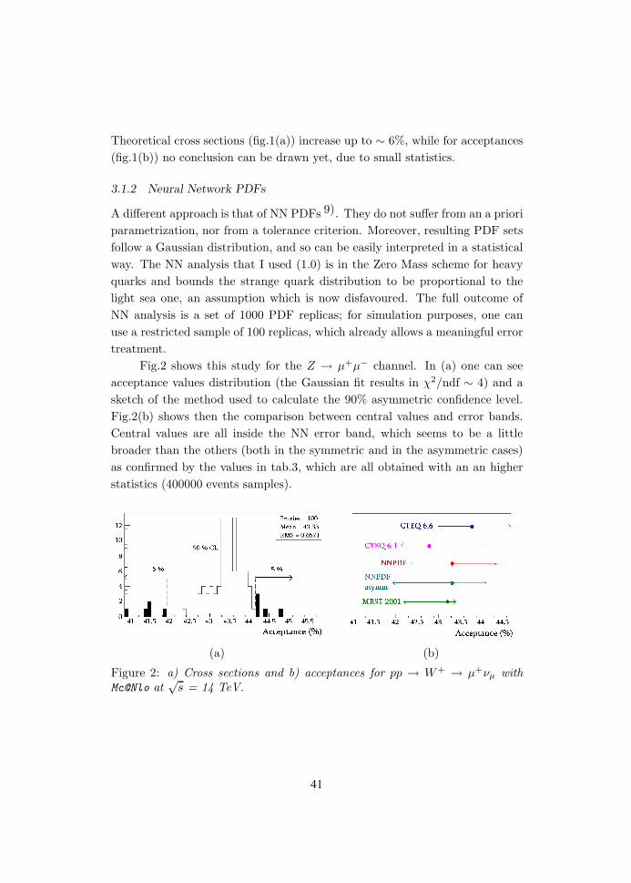
Theoretical cross sections (fig.1(a)) increase up to ∼ 6%, while for acceptances

(fig.1(b)) no conclusion can be drawn yet, due to small statistics.

3.1.2 Neural Network PDFs

A different approach is that of NN PDFs 9). They do not suffer from an a priori

parametrization, nor from a tolerance criterion. Moreover, resulting PDF sets

follow a Gaussian distribution, and so can be easily interpreted in a statistical

way. The NN analysis that I used (1.0) is in the Zero Mass scheme for heavy

quarks and bounds the strange quark distribution to be proportional to the

light sea one, an assumption which is now disfavoured. The full outcome of

NN analysis is a set of 1000 PDF replicas; for simulation purposes, one can

use a restricted sample of 100 replicas, which already allows a meaningful error

treatment.

Fig.2 shows this study for the Z → µ+µ− channel. In (a) one can see

acceptance values distribution (the Gaussian fit results in χ2/ndf ∼ 4) and a

sketch of the method used to calculate the 90% asymmetric confidence level.

Fig.2(b) shows then the comparison between central values and error bands.

Central values are all inside the NN error band, which seems to be a little

broader than the others (both in the symmetric and in the asymmetric cases)

as confirmed by the values in tab.3, which are all obtained with an an higher

statistics (400000 events samples).

(a) (b)

Figure 2: a) Cross sections and b) acceptances for pp → W+ → µ+νµ with

Mc@Nlo at√

s = 14 TeV.

41

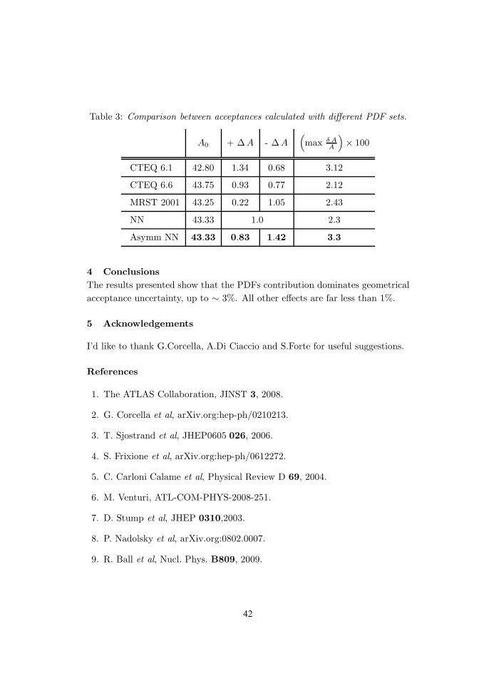
Table 3: Comparison between acceptances calculated with different PDF sets.

A0 + ∆ A - ∆ A(max δ A

A

)× 100

CTEQ 6.1 42.80 1.34 0.68 3.12

CTEQ 6.6 43.75 0.93 0.77 2.12

MRST 2001 43.25 0.22 1.05 2.43

NN 43.33 1.0 2.3

Asymm NN 43.33 0.83 1.42 3.3

4 Conclusions

The results presented show that the PDFs contribution dominates geometrical

acceptance uncertainty, up to ∼ 3%. All other effects are far less than 1%.

5 Acknowledgements

I’d like to thank G.Corcella, A.Di Ciaccio and S.Forte for useful suggestions.

References

1. The ATLAS Collaboration, JINST 3, 2008.

2. G. Corcella et al, arXiv.org:hep-ph/0210213.

3. T. Sjostrand et al, JHEP0605 026, 2006.

4. S. Frixione et al, arXiv.org:hep-ph/0612272.

5. C. Carloni Calame et al, Physical Review D 69, 2004.

6. M. Venturi, ATL-COM-PHYS-2008-251.

7. D. Stump et al, JHEP 0310,2003.

8. P. Nadolsky et al, arXiv.org:0802.0007.

9. R. Ball et al, Nucl. Phys. B809, 2009.

42

Frascati Physics Series Vol. XLVIII (2009), pp. 43-48Young Researchers Workshop: “Physics Challenges in the LHC Era”

Frascati, May 11 and 14, 2009

THE CMS MUON RECONSTRUCTION

Giorgia MilaUniversity of Turin & INFN

Abstract

One of the main goals of the Compact Muon Solenoid (CMS) design is to ensureefficient and accurate muon reconstruction.Here a general overview of the CMS track fitting method and of the muonreconstruction process is given. Muon offline data quality monitoring and muonreconstruction certification are also discussed.

1 Introduction

The Compact Muon Solenoid (CMS) experiment 1) is one of two large general-

purpose detectors for particle physics which is built at the proton-proton Large

Hadron Collider (LHC) at CERN. It consists of a cylindrical barrel closed by

two endcap disks and it is composed by four main detector subsystems. The

43

innermost system is a silicon-based tracker. A scintillating crystal electromag-

netic calorimeter surrounds it. A sampling calorimeter for hadrons is then

placed after the electromagnetic calorimeter. The tracker and the calorimetry

are compact enough to fit inside the CMS solenoid which generates a magnetic

field of 3.8 T. Outside the magnet there are the large muon detectors, which are

located inside the return yoke of the magnet. Since in a hadron collider leptons

provide a clear signature for many of the most interesting physics processes, a

precise and fast reconstruction of the leptons is mandatory for CMS. In this

context the muons play a key role because their properties can be measured

with great precision, as described in the following.

2 Track parameters and tracking algorithm principles

The CMS track reconstruction 2) is based on the Kalman Filter technique 3),

which is a recursive method for the fit of a discrete set of data. The basic

problem of this method consists in the estimation of a generic state vector x

given a set of measurements mk that are assumed to have the form

mk = Hkxk,true + εk (1)

where Hk is is the transform matrix from the state space to the measurement

space and εk is the noise that affects the true state. In the case of the track re-

construction, the state vector is defined as the position and momentum relative

to a given surface:

x =

⎛⎜⎜⎜⎜⎝q/ptanφtanθ

xy

⎞⎟⎟⎟⎟⎠ (2)

where q is the charge, p is the momentum and φ, θ, x and y identify the track

direction and position on the surface.

To complete the track description, a 5D curvilinear covariance matrix, the

number of degrees of freedom and a summary of the information on the collected

hits are stored in the corresponding data format.

The first step of the track reconstruction consists in the seed state estimation.

For muon tracks the seed can be estimated starting from the measurements

themselves or from external input. Each Kalman Filter step is then developed

by two basic components:

44

1. the propagator : it extrapolate a state vector and its covariance matrix

in a non-constant magnetic field, taking into account the effect of energy

loss and multiple scattering in the material traversed by the track.

2. the updator : it includes the information from a measurement into the

track.

The result of a Kalman filter is a state on the surface of the last measurement,

which includes all available information. However, the trajectory parameters

calculated at other points of the trajectory do not include the information from

all measurements. A second iteration is used to update the parameters at every

surface. In the Kalman filter terminology, this procedure is called smoothing.

Once the hits are fitted and the fake trajectories removed, the remaining tracks

are extrapolated to the point of closest approach to the beam line. In order to

improve the pT resolution a beam-spot constraint is possibly applied.

3 The muon reconstruction

Muon tracks in CMS are reconstructed at different levels and three different

types of high-level muons are reconstructed. The tracks within the muon sys-

tem are built combining the information coming from each muon sub-detector.

This step is the so called Stand-Alone Muon Reconstruction. In parallel (and

independently) the tracks in the tracker are reconstructed. Finally, the informa-

tion from the muon spectrometer and the tracker system are combined (Global

Muon Reconstruction) giving the final muon track. The association with the en-

ergy deposits in the calorimeters completes the muon reconstruction. Moreover

a complementary approach which considers all the silicon tracker tracks and

identifies them as muons by looking for compatible signatures in the calorimet-

ric and the muon systems has been developed (Tracker Muon Reconstruction).

3.1 Stand-Alone muons

Their reconstruction takes into account only information from the muon spec-

trometer. First track segments are reconstructed locally inside each muon

detector. Then the high-level reconstruction matches the information coming

from different detectors to perform the tracking. A pattern of compatible seg-

ments with the muon trajectory is chosen. Then a first fit using the segment

information is followed by a second more accurate fit which uses single hits

45

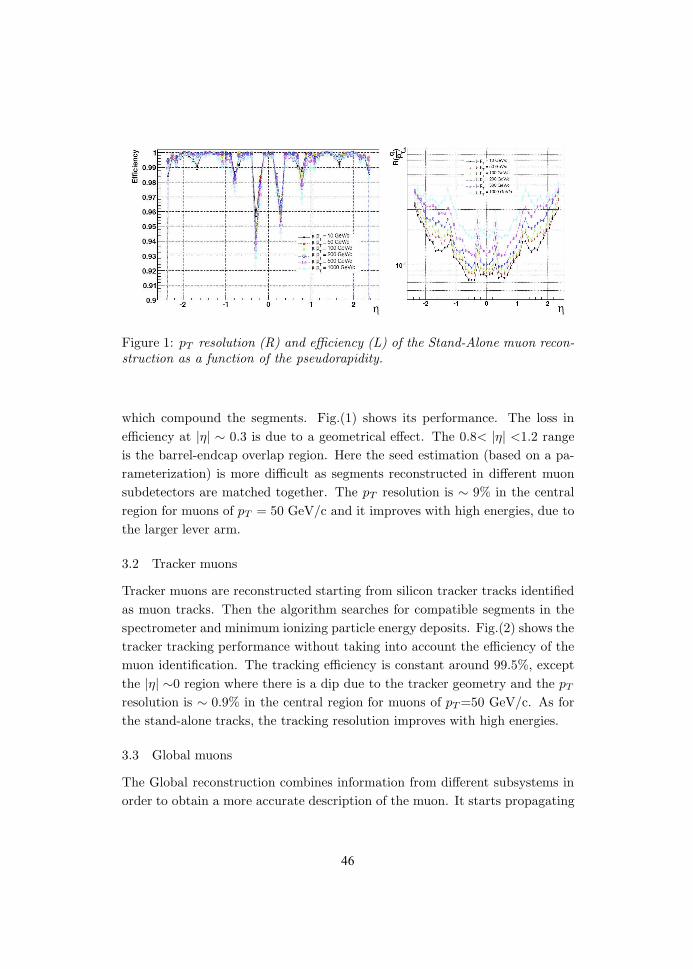
Figure 1: pT resolution (R) and efficiency (L) of the Stand-Alone muon recon-

struction as a function of the pseudorapidity.

which compound the segments. Fig.(1) shows its performance. The loss in

efficiency at |η| ∼ 0.3 is due to a geometrical effect. The 0.8< |η| <1.2 range

is the barrel-endcap overlap region. Here the seed estimation (based on a pa-

rameterization) is more difficult as segments reconstructed in different muon

subdetectors are matched together. The pT resolution is ∼ 9% in the central

region for muons of pT = 50 GeV/c and it improves with high energies, due to

the larger lever arm.

3.2 Tracker muons

Tracker muons are reconstructed starting from silicon tracker tracks identified

as muon tracks. Then the algorithm searches for compatible segments in the

spectrometer and minimum ionizing particle energy deposits. Fig.(2) shows the

tracker tracking performance without taking into account the efficiency of the

muon identification. The tracking efficiency is constant around 99.5%, except

the |η| ∼0 region where there is a dip due to the tracker geometry and the pT

resolution is ∼ 0.9% in the central region for muons of pT =50 GeV/c. As for

the stand-alone tracks, the tracking resolution improves with high energies.

3.3 Global muons

The Global reconstruction combines information from different subsystems in

order to obtain a more accurate description of the muon. It starts propagating

46

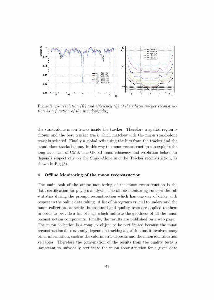
Figure 2: pT resolution (R) and efficiency (L) of the silicon tracker reconstruc-

tion as a function of the pseudorapidity.

the stand-alone muon tracks inside the tracker. Therefore a spatial region is

chosen and the best tracker track which matches with the muon stand-alone

track is selected. Finally a global refit using the hits from the tracker and the

stand-alone tracks is done. In this way the muon reconstruction can exploits the

long lever arm of CMS. The Global muon efficiency and resolution behaviour

depends respectively on the Stand-Alone and the Tracker reconstruction, as

shown in Fig.(3).

4 Offline Monitoring of the muon reconstruction

The main task of the offline monitoring of the muon reconstruction is the

data certification for physics analysis. The offline monitoring runs on the full

statistics during the prompt reconstruction which has one day of delay with

respect to the online data taking. A list of histograms crucial to understand the

muon collection properties is produced and quality tests are applied to them

in order to provide a list of flags which indicate the goodness of all the muon

reconstruction components. Finally, the results are published on a web page.

The muon collection is a complex object to be certificated because the muon

reconstruction does not only depend on tracking algorithm but it involves many

other information, such as the calorimetric deposits and the muon identification

variables. Therefore the combination of the results from the quality tests is

important to univocally certificate the muon reconstruction for a given data

47

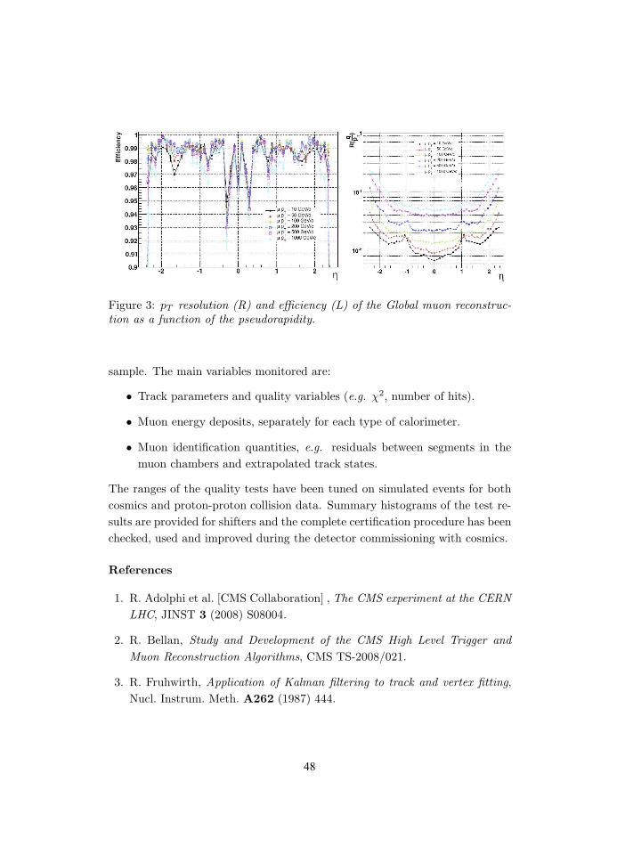
Figure 3: pT resolution (R) and efficiency (L) of the Global muon reconstruc-

tion as a function of the pseudorapidity.

sample. The main variables monitored are:

• Track parameters and quality variables (e.g. χ2, number of hits).

• Muon energy deposits, separately for each type of calorimeter.

• Muon identification quantities, e.g. residuals between segments in the

muon chambers and extrapolated track states.

The ranges of the quality tests have been tuned on simulated events for both

cosmics and proton-proton collision data. Summary histograms of the test re-

sults are provided for shifters and the complete certification procedure has been

checked, used and improved during the detector commissioning with cosmics.

References

1. R. Adolphi et al. [CMS Collaboration] , The CMS experiment at the CERN

LHC, JINST 3 (2008) S08004.

2. R. Bellan, Study and Development of the CMS High Level Trigger and

Muon Reconstruction Algorithms, CMS TS-2008/021.

3. R. Fruhwirth, Application of Kalman filtering to track and vertex fitting,

Nucl. Instrum. Meth. A262 (1987) 444.

48

Frascati Physics Series Vol. XLVIII (2009), pp. 49-54Young Researchers Workshop: “Physics Challenges in the LHC Era”

Frascati, May 11 and 14, 2009

HEAVY VECTOR PAIR PRODUCTION AT LHC IN THECHIRAL LAGRANGIAN FORMULATION

Antonio Enrique Carcamo HernandezScuola Normale Superiore Di Pisa, Pisa, Italy

Abstract

The total cross sections for Heavy vector pair production at LHC by longitu-dinal gauge boson fusion and Drell Yan annihilation are studied as a functionof the mass MV of the vector in the framework of the Chiral Lagrangian for-mulation with massive spin one fields. The cross section for V +V − productionin e+e− collisions at

√s = 3TeV is also studied.

1 Introduction

In spite of the very good agreement of the Standard Model predictions with

experimental data, the Higgs boson has not been detected experimentaly and

then the mechanism of electroweak symmetry breaking responsible for the gen-

eration of the masses of the fermions and bosons remains to be explained.

Besides that, the Standard Model does not explain the scale of the electroweak

49

symmetry breaking, which is a free parameter of the theory, taken from the ex-

periment. Moreover, the Standard model has the so called hierarchy problem,

which is the instability of the Higgs field against quantum corrections.

Since there is no experimental evidence for a Higgs particle up to date, it is

natural to ask what happens if we keep all the standard model fields, except

the Higgs boson. With this motivation and inspired in the Chiral Perturbation

Theory Lagrangian formalism up to O(p4)

developed by Ecker et al., Barbieri

et al have introduced a SU (2)L × SU (2)R Chiral Lagrangian with two mas-

sive spin one tensor fields of opposite parity which interact with the Goldstone

bosons and with the Standard Model gauge fields. This Chiral Lagrangian for-

mulation with massive spin one tensor fields of opposite parity, which is meant

to be valid up to a cutoff Λ 4πv 3TeV can account for the Electroweak

Precision Tests and keep the unitarity of the longitudinal W boson scattering

under control up to 3TeV 1). Since in the mentioned Chiral Lagrangian for-

mulation with massive spin one tensor fields, unitarity of longitudinal W boson

scattering is preserved up to 3TeV , these spin one tensor fields play the role of

the Higgs boson in keeping unitarity under control.

2 Effective Chiral Lagrangian with massive spin 1 fields.

Chiral Lagrangians have been extensively used to describe the phenomenon

of spontaneuos symmetry breaking in strong and in weak interactions. They

can be regarded as the low energy limit of an underlying fundamental theory2, 3, 4). Inspired in the Chiral Perturbation Theory Lagrangian formalism up

to O(p4)

developed by Ecker et al. used in the description of the low energy

effects in QCD, the following SU (2)L×SU (2)R invariant Lagrangian at O(p2)

describing the coupling of heavy fields V µν and Aµν to Goldstone bosons and

Standard Model gauge fields, invariant under parity is considered 1):

Leff =v2

4Tr(DµU (DµU)

†)− 1

2

∑R=V,A

Tr

(∇λRλµ∇νRνµ − 1

2M2

V RµνRµν

)+

i

2√

2GV Tr (V µν [uµ, uν ]) +

FV

2√

2Tr[V µν

(uWµνu† + u†Bµνu

)]+

FA

2√

2Tr[Aµν

(uWµνu† − u†Bµνu

)](1)

50

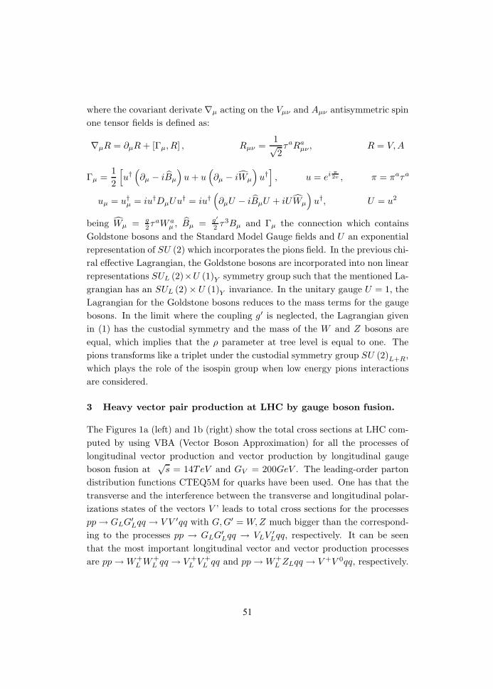
where the covariant derivate ∇µ acting on the Vµν and Aµν antisymmetric spin

one tensor fields is defined as:

∇µR = ∂µR + [Γµ, R] , Rµν =1√2τaRa

µν , R = V, A

Γµ =1

2

[u†

(∂µ − iBµ

)u + u

(∂µ − iWµ

)u†

], u = ei π

2v , π = πaτa

uµ = u†

µ = iu†DµUu† = iu†

(∂µU − iBµU + iUWµ

)u†, U = u2

being Wµ = g2τaW a

µ , Bµ = g′

2 τ3Bµ and Γµ the connection which contains

Goldstone bosons and the Standard Model Gauge fields and U an exponential

representation of SU (2) which incorporates the pions field. In the previous chi-

ral effective Lagrangian, the Goldstone bosons are incorporated into non linear

representations SUL (2)×U (1)Y symmetry group such that the mentioned La-

grangian has an SUL (2)× U (1)Y invariance. In the unitary gauge U = 1, the

Lagrangian for the Goldstone bosons reduces to the mass terms for the gauge

bosons. In the limit where the coupling g′ is neglected, the Lagrangian given

in (1) has the custodial symmetry and the mass of the W and Z bosons are

equal, which implies that the ρ parameter at tree level is equal to one. The

pions transforms like a triplet under the custodial symmetry group SU (2)L+R,

which plays the role of the isospin group when low energy pions interactions

are considered.

3 Heavy vector pair production at LHC by gauge boson fusion.

The Figures 1a (left) and 1b (right) show the total cross sections at LHC com-

puted by using VBA (Vector Boson Approximation) for all the processes of

longitudinal vector production and vector production by longitudinal gauge

boson fusion at√

s = 14TeV and GV = 200GeV . The leading-order parton

distribution functions CTEQ5M for quarks have been used. One has that the

transverse and the interference between the transverse and longitudinal polar-

izations states of the vectors V ’ leads to total cross sections for the processes

pp → GLG′

Lqq → V V ′qq with G, G′ = W, Z much bigger than the correspond-

ing to the processes pp → GLG′

Lqq → VLV ′

Lqq, respectively. It can be seen

that the most important longitudinal vector and vector production processes

are pp → W+L W+

L qq → V +L V +

L qq and pp → W+L ZLqq → V +V 0qq, respectively.

51

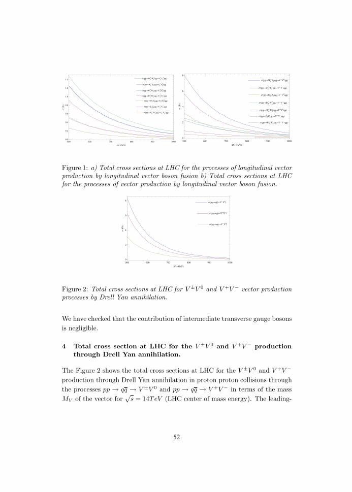
ΣppWLZLqqVL

VL0qq

ΣppWLWL

qqVLVLqq

ΣppWLWL

qqVL0VL

0qq

ΣppWLWL

qqVLVLqq

ΣppWLZLqqVL

VL0qq

ΣppZLZLqqVLVLqq

ΣppWLWL

qqVLVLqq

500 600 700 800 900 10000.0

0.2

0.4

0.6

0.8

1.0

1.2

1.4

MV GeV

Σf

b

ΣppWLZLqqVV0qq

ΣppWLWL

qqVVqq

ΣppWLZLqqVV0qq

ΣppWLWL

qqVVqq

ΣppWLWL

qqV0V0qq

ΣppZLZLqqVVqq

ΣppWLWL

qqVVqq

500 600 700 800 900 10000

2

4

6

8

MV GeV

Σf

b

Figure 1: a) Total cross sections at LHC for the processes of longitudinal vector

production by longitudinal vector boson fusion b) Total cross sections at LHC

for the processes of vector production by longitudinal vector boson fusion.

ΣppqqVV0

ΣppqqVV

ΣppqqVV0

500 600 700 800 900 10000

2

4

6

8

MV GeV

Σf

b

Figure 2: Total cross sections at LHC for V ±V 0 and V +V − vector production

processes by Drell Yan annihilation.

We have checked that the contribution of intermediate transverse gauge bosons

is negligible.

4 Total cross section at LHC for the V ±V 0 and V +V − productionthrough Drell Yan annihilation.

The Figure 2 shows the total cross sections at LHC for the V ±V 0 and V +V −

production through Drell Yan annihilation in proton proton collisions through

the processes pp → qq → V ±V 0 and pp → qq → V +V − in terms of the mass

MV of the vector for√

s = 14TeV (LHC center of mass energy). The leading-

52

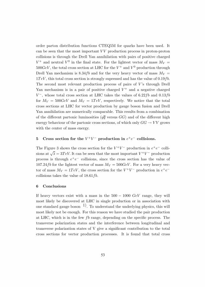
order parton distribution functions CTEQ5M for quarks have been used. It

can be seen that the most important V V production process in proton-proton

collisions is through the Drell Yan annihilation with pairs of positive charged

V + and neutral V 0 in the final state. For the lightest vector of mass MV =

500GeV , the total cross section at LHC for the V + and V 0 production through

Drell Yan mechanism is 8.34fb and for the very heavy vector of mass MV =

1TeV , this total cross section is strongly supressed and has the value of 0.19fb.

The second most relevant production process of pairs of V ’s through Drell

Yan mechanism is in a pair of positive charged V + and a negative charged

V −, whose total cross section at LHC takes the values of 6.22fb and 0.13fb

for MV = 500GeV and MV = 1TeV , respectively. We notice that the total

cross sections at LHC for vector production by gauge boson fusion and Drell

Yan annihilation are numerically comparable. This results from a combination

of the different partonic luminosities (qq versus GG) and of the different high

energy behaviour of the partonic cross sections, of which only GG → V V grows

with the center of mass energy.

5 Cross section for the V +V − production in e+e− collisions.

The Figure 3 shows the cross section for the V +V − production in e+e− colli-

sions at√

s = 3TeV. It can be seen that the most important V +V − production

process is through e+e− collisions, since the cross section has the value of

107.24fb for the lightest vector of mass MV = 500GeV . For a very heavy vec-

tor of mass MV = 1TeV , the cross section for the V +V − production in e+e−

collisions takes the value of 18.61fb.

6 Conclusions

If heavy vectors exist with a mass in the 500 − 1000 GeV range, they will

most likely be discovered at LHC in single production or in association with

one standard gauge boson 1). To understand the underlying physics, this will

most likely not be enough. For this reason we have studied the pair production

at LHC, which is in the few fb range, depending on the specific process. The

transverse polarization states and the interference between longitudinal and

transverse polarization states of V give a significant contribution to the total

cross sections for vector production processes. It is found that total cross

53

500 600 700 800 900 1000

20

40

60

80

100

MV GeV

Σf

b

Figure 3: Total cross sections for the V +V − production in e+e− collisions

sections at LHC for vector production and Drell Yan annihilation have similar

values and that the most relevant vector production processes corresponds to

a pair of positive charged and neutral vectors in the final state. It is also

important to mention that charged vector production process in e+e− collisions

is very promising. Further detailed studies will have to be made to assess the

detectability of these processes above the Standard Model backgrounds.

7 Acknowledgements

The author thanks Professor Riccardo Barbieri for introducing him to this field,

for carefully reading of the article and for very useful discussions. Author also

thanks R. Torres, G. Corcella and R. Trincherini for very useful discussions.

References

1. R. Barbieri, G. Isidori, V. S. Rychkov and E. Trincherini, Phys. Rev. D 78,

036012 (2008) [arXiv:hep-ph/0806.1624v1].

2. G. Ecker et al, Phys. Rev. Lett. B 223 (1989) 425; Nucl. Phys. B 321

(1989) 311

3. A. V. Manohar, arXiv:hep-ph/9606222v1.

4. A. Pich, arXiv:hep-ph/9806303v1.

54

Frascati Physics Series Vol. XLVIII (2009), pp. 55-60Young Researchers Workshop: “Physics Challenges in the LHC Era”

Frascati, May 11 and 14, 2009

MASS DEGENERATE HEAVY VECTOR MESONS ATHADRON COLLIDERS

Mark RoundSwansea University, School of Physical Sciences,

Singleton Park, Swansea, Wales, UK

Abstract

We study the LHC phenomenology of two mass-degenerate heavy gauge bosonswith the quantum numbers of the Z and γ. We give a leading-order estimateof the number of events expected in Drell-Yan processes in terms of the modeland machine parameters. We consider the feasibility of measuring a forward-backward asymmetry for various choices of the parameters and estimate thereach. We comment on how the results may affect future collider design.

1 Introduction

The main purpose of the LHC is to discover the origin of electro-weak (EW)

symmetry breaking and what new physics lies at the TeV scale.

One clean signal for the LHC would be the discovery of new, higher-mass

copies of the standard-model (SM) gauge fields. For such a scenario, the LHC

55

reach in observable masses and couplings is of interest. Motivations for this

study include weakly coupled SM extensions with new heavy vector fields 1),

little Higgs models 2) and technicolor (TC) 3).

In this paper, we consider the scenario in which a complete set of four spin-

1 copies of the SM gauge bosons with heavy degenerate masses are produced

in pp collisions and detected via the decay into muons. The muon channel is

expected to have a low background at the LHC. For simplicity, we model the

decay width of these particles by assuming it to be dominated by the decay into

SM fermions, hence avoiding complications (and model-dependencies) arising

when including the decay into light scalars and gauge bosons.

In the SM, a forward-backward asymmetry arises from interference terms

between virtual processes with the exchange of Z and γ, and it is a very sizable

effect even in the TeV energy range. Measuring such an effect at a hadron

collider is onerous but a method and its use at the LHC was surveyed by

Dittmar 4). Measuring an asymmetry at a new neutral pole would indicate it

is made of two different exchange particles.

2 Model Phenomenology

We model the new neutral resonances by adding an extra set of SU(2)×U(1)

gauge fields into the SM electro-weak Lagrangian. We assume that some mech-

anism spontaneously breaks the SU(2)2 × U(1)2 gauge symmetry to the SM

SU(2)L × U(1)Y above the TeV scale, and that in the process a copy of the

W , Z and γ all aquire a similar mass m. We also assume that the couplings

of the heavy gauge bosons to the SM currents can be written as RgSM , where

gSM stands for the coupling of the W , Z and γ. The common mass, m, and

the coupling ratio R are the only parameters.

In this scenario one can compute the Drell-Yan event rate, N , with a

PDF package and indeed, it can be approximated by 5),

N ∝ sLR

m4, (1)

up to a proportionality constant that contains the electro-weak couplings and

the normalization of the PDF distribution. For this study we used the Fermi02

set 6) & 7).

Discovery of the new resonance depends on some value of the ratio N/L

of the event number N and the machine luminosity L. The approximate event

56

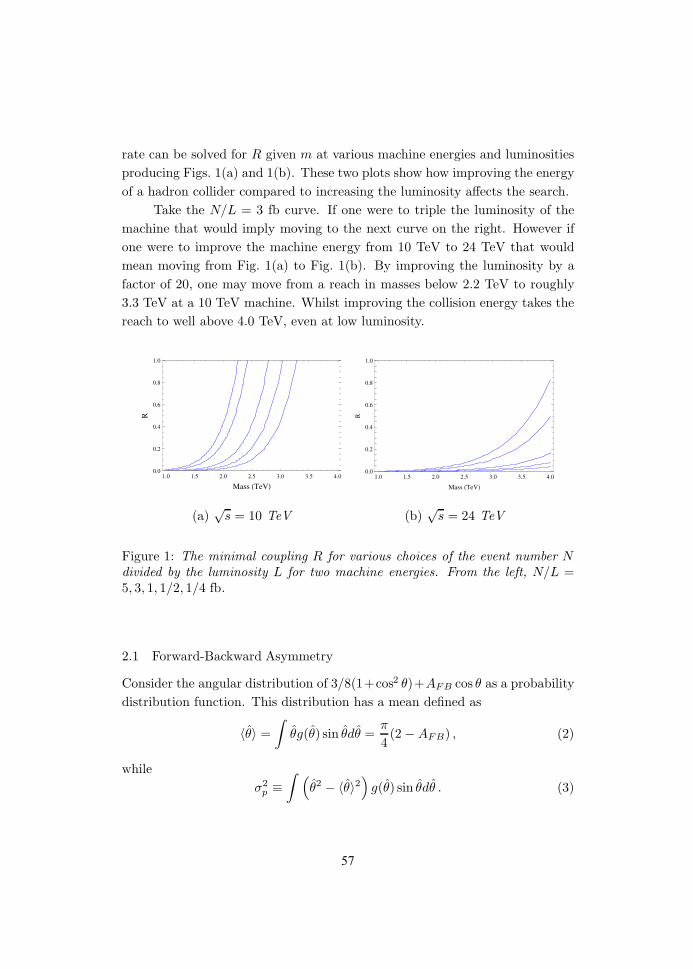
rate can be solved for R given m at various machine energies and luminosities

producing Figs. 1(a) and 1(b). These two plots show how improving the energy

of a hadron collider compared to increasing the luminosity affects the search.

Take the N/L = 3 fb curve. If one were to triple the luminosity of the

machine that would imply moving to the next curve on the right. However if

one were to improve the machine energy from 10 TeV to 24 TeV that would

mean moving from Fig. 1(a) to Fig. 1(b). By improving the luminosity by a

factor of 20, one may move from a reach in masses below 2.2 TeV to roughly

3.3 TeV at a 10 TeV machine. Whilst improving the collision energy takes the

reach to well above 4.0 TeV, even at low luminosity.

1.0 1.5 2.0 2.5 3.0 3.5 4.00.0

0.2

0.4

0.6

0.8

1.0

Mass TeV

R

(a)√

s = 10 TeV

1.0 1.5 2.0 2.5 3.0 3.5 4.00.0

0.2

0.4

0.6

0.8

1.0

Mass TeV

R

(b)√

s = 24 TeV

Figure 1: The minimal coupling R for various choices of the event number Ndivided by the luminosity L for two machine energies. From the left, N/L =5, 3, 1, 1/2, 1/4 fb.

2.1 Forward-Backward Asymmetry

Consider the angular distribution of 3/8(1+cos2 θ)+AFB cos θ as a probability

distribution function. This distribution has a mean defined as

〈θ〉 =

∫θg(θ) sin θdθ =

π

4(2 − AFB) , (2)

while

σ2p ≡

∫ (θ2 − 〈θ〉2

)g(θ) sin θdθ . (3)

57

Interestingly, AFB turns out to be just proportional to 〈θ〉. Hence we can

estimate the statistical error on the extraction of the symmetry as

∆AstatFB =

4σp

π√

n − 1, (4)

where n is the number of events used to study the angular distribution.

Secondly there is an error introduced by the methodology (see 4)). The

assumption that the initial quark direction be always the one of the outcoming

γ′ or Z ′, implies a possible misidentification θ ↔ π − θ. Let the probability of

mis-identification be p, then in a sample of n events np are mis-identified. Let

nF (nB) events travel in the forward (backward) direction. Then n = nF +nB.

The worst case scenario would be that all np events were placed in nF but

should have been placed in nB. In this case the difference in true and measured

asymmetry would be,

∆AsysFB = ±2p (5)

This means that adding the method and statistical errors together the total

error wil be,

∆AFB =4σp

π√

n − 1+ 2p(Yc), (6)

where the dependence of p on the cut Yc has been added for clarity. We

conservatively add the two sources of error linearly.

Now we can define P (Yc), the fraction of events with |Y | > Yc. Then, the

number of events used to extract the asymmetry is,

n = PN. (7)

Requiring that ∆AFB < E (for E > 2p) implies

n >

(4σpop

π(E − 2p

)2

+ 1 (8)

or equivalently,

N >1

P

[(4σpop

π(E − 2p

)2

+ 1

](9)

total events.

For the model considered, the asymmetry is AFB −0.42 5). The asym-

metry with the SM particles and one new resnonance is very small. Therefore

58

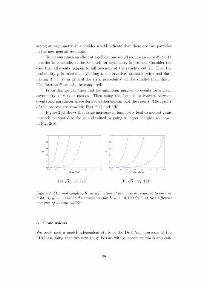
seeing an asymmetry at a collider would indicate that there are two particles

in the new neutral resonance.

To measure such an effect at a collider one would require an error E < 0.14

in order to conclude, at the 3σ level, an asymmetry is present. Consider the

case that all events happen to fall precisely at the rapidity cut Yc. Then the

probability p is calculable, yielding a conservative estimate: with real data

having |Y | > Yc in general the error probability will be smaller than this p.

The fraction P can also be computed.

From this we can then find the minimum number of events for a given

asymmetry at various masses. Then using the formula to convert between

events and parameter space derived earlier we can plot the results. The results

of this process are shown in Figs. 2(a) and 2(b).

Figure 2(a) shows that large increases in luminosity lead to modest gains

in reach, compared to the gain obtained by going to larger energies, as shown

in Fig. 2(b).

0.5 1.0 1.5 2.0 2.5 3.0 3.5 4.00.0

0.2

0.4

0.6

0.8

1.0

Mass TeV

R

(a)√

s =14 TeV

0.5 1.0 1.5 2.0 2.5 3.0 3.5 4.00.0

0.2

0.4

0.6

0.8

1.0

Mass TeV

R

(b)√

s =24 TeV

Figure 2: Minimal coupling R, as a function of the mass m, required to observe

a 3σ AFB ∼ −0.42 at the resonance for L = 1, 10, 100 fb−1 at two different

energies of hadron collider

3 Conclusions

We performed a model-independent study of the Drell-Yan processes at the

LHC, assuming that two new gauge bosons with quantum numbers and cou-

59

plings analogous to the photon and Z boson, but rescaled by a common factor

of R < 1, have masses so close to each other that their kinematic peaks are

indistinguishable.

For a 10 TeV collider, and luminosities in the 2− 40fb−1, bounds on new

resonances no higher than 3 TeV can be obtained. With a 24 TeV collider the

region well over 4 TeV can be explored, depending on the specific coupling R.

As for the forward-backward asymmetry, we provided a simple estimate

formula that ignored experimental issues. The collider ability to measure an

asymmetry at the 3σ level is heavily restricted to light masses. Even at very

high luminosities measuring the asymmetry for masses of 3 TeV is out of reach

for a 14 TeV collider, even in principle. By contrast, at a 24 TeV machine

the reach is far larger. This is as a result of the PDF scaling offering a larger

fraction of high rapidity events with higher energy. At such a machine it may be

possible to measure asymmetries and greatly restrict currently open parameter

spaces.

4 Acknowledgements

The author wishes to thank M. Piai for useful comments on the manuscript.

References

1. See for instance T. Appelquist, B. A. Dobrescu and A. R. Hopper, Phys.

Rev. D 68, 035012 (2003) [arXiv:hep-ph/0212073], and references therein.

2. See for instance N. Arkani-Hamed, A. G. Cohen, E. Katz and A. E. Nelson,

JHEP 0207, 034 (2002) [arXiv:hep-ph/0206021]; I. Low, W. Skiba and

D. Tucker-Smith, Phys. Rev. D 66, 072001 (2002) [arXiv:hep-ph/0207243].

3. S. Weinberg, Phys. Rev. D 19, 1277 (1979); L. Susskind, Phys. Rev. D 20,

2619 (1979); S. Weinberg, Phys. Rev. D 13, 974 (1976).

4. M. Dittmar, Phys. Rev. D 55, 161 (1997) [arXiv:hep-ex/9606002].

5. M. Piai and M. Round, arXiv:0904.1524 [hep-ph].

6. M. R. Whalley, D. Bourilkov and R. C. Group, arXiv:hep-ph/0508110.

7. W. T. Giele, S. A. Keller and D. A. Kosower, arXiv:hep-ph/0104052.

60

Frascati Physics Series Vol. XLVIII (2009), pp. 61-66Young Researchers Workshop: “Physics Challenges in the LHC Era”

Frascati, May 11 and 14, 2009

STUDY OF B → Kηc AND B → Kηc(2S) DECAYS

Anna Vinokurova (for the Belle collaboration)Budker Institute of Nuclear Physics

Abstract

A data sample of 535 million BB meson pairs collected in the Belle experimentat the KEKB e+e- collider has been used to study properties of the ηc andits excited state ηc(2S) mesons produced in B decay to K and charmonium.We use the decay of charmonium to KSKπ to study the effects of interferencebetween signal events and events of the B decay into the same final statewithout intermediate charmonium. Taking this interference into account weobtain masses, widths, and decay branching fractions of the ηc and ηc(2S)mesons. The results agree with the world average values and for the first timethe intereference effects are taken into account.

1 Introduction

The decay B± → K±cc is a copious source of charmonia. The ηc branching

fractions were measured with poor accuracy and can be improved. The ηc(2S)

61

meson was seen in one hadronic decay only (ηc(2S) → KSK±π∓) and requires

some additional study. It can be easily done using the analysis algorithm similar

to the one for ηc. The following decays of B mesons were studied:

B± → K±ηc → K±KSK±π∓, (1)

B± → K±ηc(2S) → K±KSK±π∓. (2)

The analysis was performed using the Belle detector 1). Considered statis-

tics is rather high – 492 fb−1 and gives an opportunity to determine masses

and widths of ηc and ηc(2S) mesons.

2 Event selection

A data sample of 492 fb−1 (535 million BB events) collected at the Υ(4S)

resonance is used in this analysis. In this analysis K candidates decay via the

π+π− mode.

Charged tracks are selected with requirements based on the average hit

residuals and impact parameters relative to the interaction point. We require

that the polar angle of each track be in the angular range of 18 − 152 and

that the track transverse momentum be greater than 100 MeV/c.

Charged kaon candidates are identified by the requirement R(K) > 0.6,

which has an efficiency of 90% and a pion misidentification probability of ap-

proximately (3 − 10)%. For pion candidates we require R(π) > 0.2.

B meson candidates are identified by their center-of-mass (c.m.) energy

difference ∆E = (∑

i Ei) − Eb, and the beam-constrained mass

Mbc =√

E2b − (

∑i pi)2, where Eb =

√s/2 is the beam energy in the Υ(4S)

c.m. frame, and pi and Ei are the c.m. three-momenta and energies, respectively

of the B meson candidate decay products.

To suppress the large continuum background (e+e− → qq, where q =

u, d, s, c), topological variables are used. Since the produced B mesons are al-

most at rest in the c.m. frame, the signal event shapes tend to be isotropic

while continuum qq events tend to have a two-jet structure. We use the an-

gle between the thrust axis of the B candidate and that of the rest of the

event (Θthrust) to discriminate between these two cases. The distribution of

| cosΘthrust| is strongly peaked near | cosΘthrust| = 1 for qq events and is nearly

flat for Υ(4S) → BB events. We require | cosΘthrust| < 0.8.

62

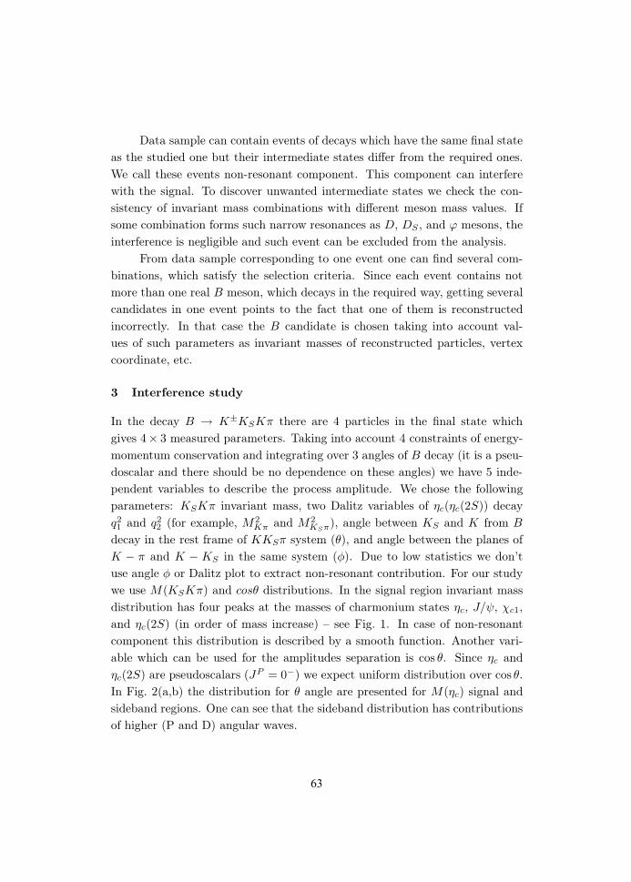
Data sample can contain events of decays which have the same final state

as the studied one but their intermediate states differ from the required ones.

We call these events non-resonant component. This component can interfere

with the signal. To discover unwanted intermediate states we check the con-

sistency of invariant mass combinations with different meson mass values. If

some combination forms such narrow resonances as D, DS , and ϕ mesons, the

interference is negligible and such event can be excluded from the analysis.

From data sample corresponding to one event one can find several com-

binations, which satisfy the selection criteria. Since each event contains not

more than one real B meson, which decays in the required way, getting several

candidates in one event points to the fact that one of them is reconstructed

incorrectly. In that case the B candidate is chosen taking into account val-

ues of such parameters as invariant masses of reconstructed particles, vertex

coordinate, etc.

3 Interference study

In the decay B → K±KSKπ there are 4 particles in the final state which

gives 4× 3 measured parameters. Taking into account 4 constraints of energy-

momentum conservation and integrating over 3 angles of B decay (it is a pseu-

doscalar and there should be no dependence on these angles) we have 5 inde-

pendent variables to describe the process amplitude. We chose the following

parameters: KSKπ invariant mass, two Dalitz variables of ηc(ηc(2S)) decay

q21 and q2

2 (for example, M2Kπ and M2

KSπ), angle between KS and K from B

decay in the rest frame of KKSπ system (θ), and angle between the planes of

K − π and K − KS in the same system (φ). Due to low statistics we don’t

use angle φ or Dalitz plot to extract non-resonant contribution. For our study

we use M(KSKπ) and cosθ distributions. In the signal region invariant mass

distribution has four peaks at the masses of charmonium states ηc, J/ψ, χc1,

and ηc(2S) (in order of mass increase) – see Fig. 1. In case of non-resonant

component this distribution is described by a smooth function. Another vari-

able which can be used for the amplitudes separation is cos θ. Since ηc and

ηc(2S) are pseudoscalars (JP = 0−) we expect uniform distribution over cos θ.

In Fig. 2(a,b) the distribution for θ angle are presented for M(ηc) signal and

sideband regions. One can see that the sideband distribution has contributions

of higher (P and D) angular waves.

63

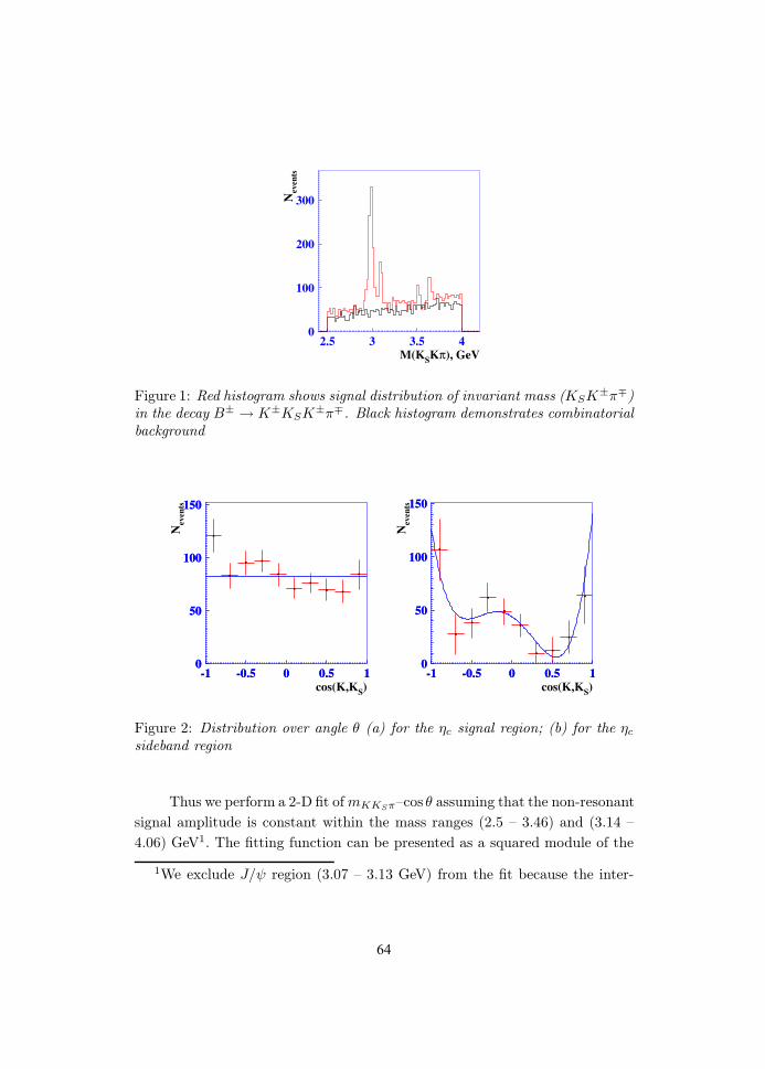
0

100

200

300

2.5 3 3.5 4M(KSKπ), GeV

Nev

ents

Figure 1: Red histogram shows signal distribution of invariant mass (KSK±π∓)in the decay B± → K±KSK±π∓. Black histogram demonstrates combinatorialbackground

0

50

100

150

-1 -0.5 0 0.5 10

50

100

150

-1 -0.5 0 0.5 1cos(K,KS)

Nev

ents

0

50

100

150

-1 -0.5 0 0.5 10

50

100

150

-1 -0.5 0 0.5 1cos(K,KS)

Nev

ents

Figure 2: Distribution over angle θ (a) for the ηc signal region; (b) for the ηc

sideband region

Thus we perform a 2-D fit of mKKSπ–cos θ assuming that the non-resonant

signal amplitude is constant within the mass ranges (2.5 – 3.46) and (3.14 –

4.06) GeV1. The fitting function can be presented as a squared module of the

1We exclude J/ψ region (3.07 – 3.13 GeV) from the fit because the inter-

64

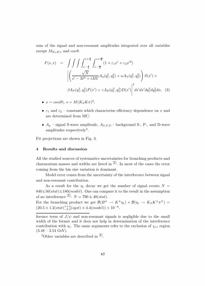
sum of the signal and non-resonant amplitudes integrated over all variables

except MKSKπ and cos θ:

F (s, x) =

∫ ∫ ∫ ∫ x+ δ2

x− δ2

∫ s+ ∆2

s−∆2

(1 + ε1x′ + ε2x

′2)∣∣∣∣∣( √

N

s′ − M2 + iMΓAη(q2

1 , q22) + αAS(q2

1 , q22)

)S(x′) +

βAP (q21 , q

22)P (x′) + γAD(q2

1 , q22)D(x′)

∣∣∣∣∣2

ds′dx′dq21dq2

2dφ, (3)

• x = cos(θ), s = M(KSKπ)2;

• ε1 and ε2 – constants which characterise efficiency dependence on x and

are determined from MC;

• Aη – signal S-wave amplitude, AS,P,D - background S-, P-, and D-wave

amplitudes respectively2.

Fit projections are shown in Fig. 3.

4 Results and discussion

All the studied sources of systematics uncertainties for branching products and

charmonium masses and widths are listed in 2). In most of the cases the error

coming from the bin size variation is dominant.

Model error comes from the uncertainty of the interference between signal

and non-resonant contribution.

As a result for the ηc decay we get the number of signal events N =

840±50(stat)±180(model). One can compare it to the result in the assumption

of no interference 2): N = 790 ± 40(stat).

For the branching product we get B(B± → K±ηc) × B(ηc → KSK±π∓) =

(20.5 ± 1.2(stat)+1.4−2.2(syst) ± 4.4(model)) × 10−6.

ference term of J/ψ and non-resonant signals is negligible due to the smallwidth of the former and it does not help in determination of the interferencecontribution with ηc. The same arguments refer to the exclusion of χc1 region(3.48 – 3.54 GeV).

2Other variables are described in 2).

65

0

50

100

150

2.6 2.8 3 3.2 3.4M(KSKπ), GeV

0

25

50

75

3.2 3.4 3.6 3.8 4M(KSKπ), GeV

Nev

ents

Figure 3: Projections of the fits of the distributions over KSKπ invariant massin ηc and ηc(2S) mass regions

Parameters of the ηc meson:

M = (2984.2± 1.2(stat)+0−1.8(syst) ± 0.2(model)) MeV;

Γ = (30.7 ± 2.3(stat)+0.4−1.2(syst) ± 0.4(model)) MeV.

Similarly, for the ηc(2S) decay we obtain N = 102±26(stat)±38(model).

In the assumption of no interference the number of events is N = 130±30(stat).

The branching product is B(B± → K±ηc(2S)) × B(ηc(2S) → KSK±π∓) =

(2.2 ± 0.6(stat)+0.6−0.1(syst) ± 0.8(model)) × 10−6.

Parameters of the ηc(2S) meson:

M = (3638.2± 2.3(stat)+1.3−2.4(syst) ± 0.8(model)) MeV;

Γ = (6.0+13.3−1.4 (stat)+8.1

−0.8(syst) ± 2.5(model)) MeV.

5 Acknowledgments

I thank the KEKB group for the excellent operation of the accelerator and my

colleagues from the Belle collaboration for numerous useful discussions.

References

1. A. Abashian et al. (Belle Collaboration), Nucl. Instr. and Meth. A 479,

117 (2002).

2. To be published.

66

Frascati Physics Series Vol. XLVIII (2009), pp. 67-72Young Researchers Workshop: “Physics Challenges in the LHC Era”

Frascati, May 11 and 14, 2009

CONTINUUM SUPPRESSION IN THERECONSTRUCTION OF B0 → π0π0

T. Danger JuliusThe University of Melbourne Parkville, Victoria Australia 3010

Abstract

This proceeding explores the improvement of the measurement of the branchingfraction of B → π0π0 , and how it is possible to tighten the bound on the angleφ2, a parameter that describes CP violation within the Standard Model.

1 CP Violation

The weak eigenstate of a quark is not its mass eigenstate, but the relationship

between the two can be expressed using the 3x3 Cabibbo-Kobayashi-Maskawa

(CKM) matrix. This matrix is unitary and contains a complex phase that can

accomodate CP violation within the Standard Model (SM).

67

⎛⎝ dsb

⎞⎠ =

⎛⎝ Vud Vus Vub

Vcd Vcs Vcb

Vtd Vts Vtb

⎞⎠⎛⎝ d′

s′

b′

⎞⎠ (1)

Equation 1 shows the CKM matrix with primed values representing the

mass eigenstates, and unprimed representing the weak eigenstates. The rela-

tionship between entries the elements of the matrix can be represented graph-

ically as a triangle on the complex plane, with angles representing the relative

phases between matrix elements. By finding the magnitudes of the sides and

the angles of this triangle, we can test the predictions of the SM, and perhaps

uncover new physics. The angle φ2, or α, is defined to be arg[−VudV ∗

ub

VtdV ∗

tb

], and

can be studied using neutral B decays.

B0 mesons are not formed by a single CP eigenstate. They are a combi-

nation of CP-odd and CP-even eigenstates. B0 and B0 can decay to a given

eigenstate f , either directly or through mixing. Over time the mixing prob-

ability changes causing the decay amplitude to change. The time dependant

decay rate of B0 meson to a fianl state f is given by

Γ(B0(t) → f) = e−Γ|t|[(|Af |2 + |Af |2) − (|Af |2 − |Af |2) (2)

cos(∆mt) + 2|Af |2Im(λf )sin(∆mt)]

where Af and Af are the respective amplitudes of B0 → f and B0 → f ,

and λf is the mixing parameter, e−ΦMAf

Afwhere ΦM is the mixing angle between

B0 and B0 1). Once the time dependant decay rates have been measured, the

CP asymmetry is calculated as a = Γ(B0→f)−Γ(B0→f)

Γ(B0→f)+Γ(B0→f).

2 Measuring B → π+π−

All B → ππ decays proceed through the b → uud quark subprocess. B0 →π+π− can proceed via the tree-level process shown in figure 1, with a branching

fraction proportional to |V ∗2ub V 2

ud|. This leads to the asymmetry

68

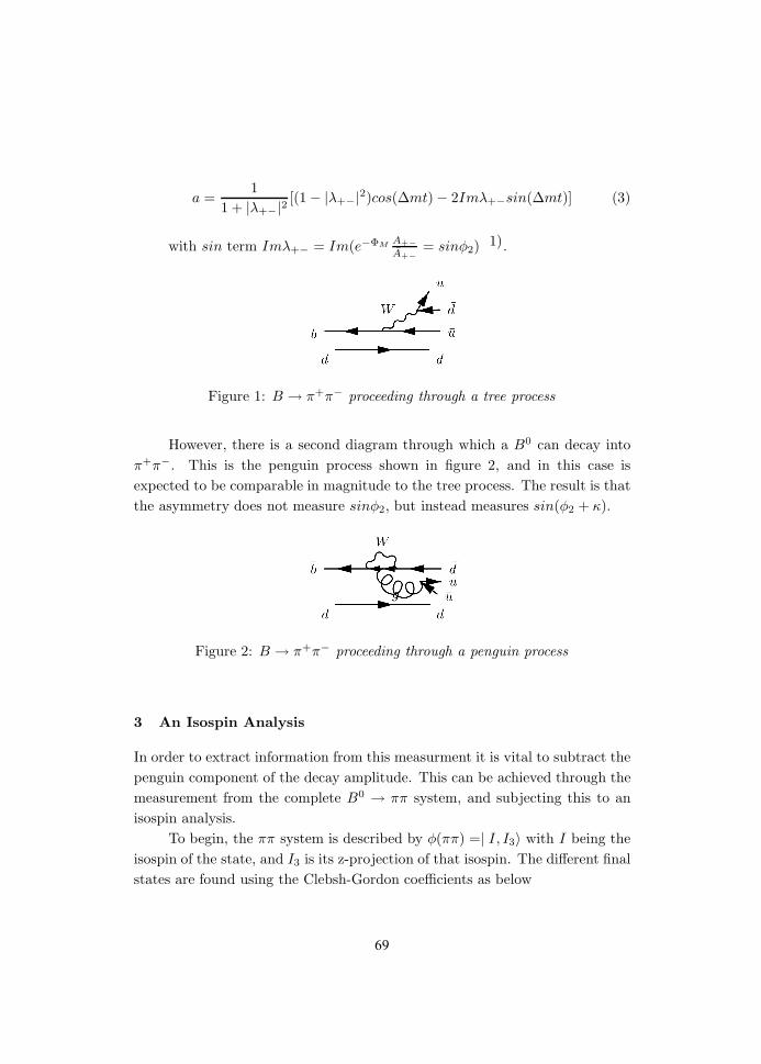
a =1

1 + |λ+−|2 [(1 − |λ+−|2)cos(∆mt) − 2Imλ+−sin(∆mt)] (3)

with sin term Imλ+− = Im(e−ΦMA+−

A+−

= sinφ2)1).

Figure 1: B → π+π− proceeding through a tree process

However, there is a second diagram through which a B0 can decay into

π+π−. This is the penguin process shown in figure 2, and in this case is

expected to be comparable in magnitude to the tree process. The result is that

the asymmetry does not measure sinφ2, but instead measures sin(φ2 + κ).

Figure 2: B → π+π− proceeding through a penguin process

3 An Isospin Analysis

In order to extract information from this measurment it is vital to subtract the

penguin component of the decay amplitude. This can be achieved through the

measurement from the complete B0 → ππ system, and subjecting this to an

isospin analysis.

To begin, the ππ system is described by φ(ππ) =| I, I3〉 with I being the

isospin of the state, and I3 is its z-projection of that isospin. The different final

states are found using the Clebsh-Gordon coefficients as below

69

Table 1: Relative amplitudes of B → ππ.

A(B+ → π+π0) =√

32 A 3

2,2

1√

2A(B0 → π+π−) = 1

√12

A 32,2 − 1

√6A 1

2,0

A(B0 → π0π0) = 1√

3A 3

2,2 − 1

√6A 1

2,0

φ(π0π0) = | 1, 0〉 | 1, 0〉 =√

23 | 2, 0〉 −

√12 | 0, 0, 〉 (4)

φ(π0π+) = | 1, 0〉 | 1, +1〉 =| 2, +1〉φ(π+π−) = | 1, +1〉 | 1,−1〉 =

√13 | 2, 0〉 +

√23 | 0, 0, 〉

At the quark level we have φ(B → uud) = A 32| 3

2 , + 12 〉 + A 1

2| 1

2 , + 12 〉.

The amplitudes of the isospin 32 and 1

2 components, A 32

and A 12, are the

unknowns to be extracted. Finally, the initial state is φ(B0) =| 12 ,− 1

2 〉. If we

apply the transition to the initial state we find

φ(b → uud)φ(B0) = A 32| 3

2, +

1

2〉 + A 1

2| 1

2, +

1

2〉 | 1

2,−1

2〉 (5)

=

√1

2A 3

2| 2, 0〉 +

√1

2(A 1

2+ A 3

2) | 1, 0〉+

√12

A 12

| 0, 0〉

The π0pi0 final state is described in equation 6.

Br(B0 → π0π0) = (√

23 〈2, 0 | −

√12 〈0, 0, |)(

√12A 3

2

| 2, 0〉 (6)

+√

12 (A 1

2+ A 3

2) | 1, 0〉 +

√12A 1

2| 0, 0〉)

=√

13A 3

2+√

16A 1

2

This is done for all three final states, the results of which are found in

table 1. For convenience two new constants are defined so that A0 =√

16 and

A2 =√

112 . Theses amplitudes relate to ∆I = 0 and ∆I = 2 respectively, and

simplify the above relations to those of equation 7.

70

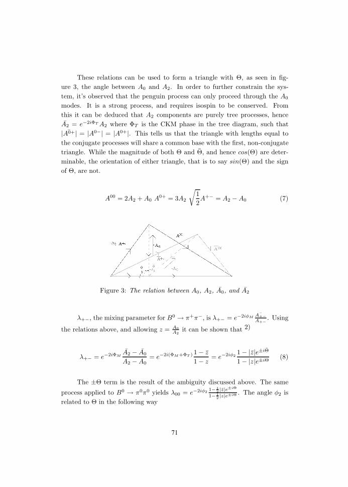
These relations can be used to form a triangle with Θ, as seen in fig-

ure 3, the angle between A0 and A2. In order to further constrain the sys-

tem, it’s observed that the penguin process can only proceed through the A0

modes. It is a strong process, and requires isospin to be conserved. From

this it can be deduced that A2 components are purely tree processes, hence

A2 = e−2iΦT A2 where ΦT is the CKM phase in the tree diagram, such that

| ¯A0+| = |A0−| = |A0+|. This tells us that the triangle with lengths equal to

the conjugate processes will share a common base with the first, non-conjugate

triangle. While the magnitude of both Θ and Θ, and hence cos(Θ) are deter-

minable, the orientation of either triangle, that is to say sin(Θ) and the sign

of Θ, are not.

A00 = 2A2 + A0 A0+ = 3A2

√1

2A+− = A2 − A0 (7)

Figure 3: The relation between A0, A2, A0, and A2

λ+−, the mixing parameter for B0 → π+π−, is λ+− = e−2iφM¯A+−

A+−

. Using

the relations above, and allowing z = A0

A2it can be shown that 2)

λ+− = e−2iΦMA2 − A0

A2 − A0= e−2i(ΦM+ΦT ) 1 − z

1 − z= e−2iφ2

1 − |z|e±iΘ

1 − |z|e±iΘ(8)

The ±Θ term is the result of the ambiguity discussed above. The same

process applied to B0 → π0π0 yields λ00 = e−2iφ21− 1

2|z|e±iΘ

1− 12|z|e±iΘ . The angle φ2 is

related to Θ in the following way

71

sin(2φ2 + κ00) = Im(λ00)|1 − 1

2 |z|e±2iΘ

1 − 12 |z|e±2iΘ

| (9)

sin(2φ2 + κ+−) = Im(λ+−)|1 − |z|e±2iΘ

1 − |z|e±2iΘ| (10)

where κ is the penguin pollution in each process. Each of equations 9

and 10 have four solutions for φ2. The solutions that overlap between the two

equations determine φ2 if individual measurements of A00, A00, A+−, and ¯A+−

are availible, However, this can be experimentally difficult, as it’s difficult to

distinguish B0 → π0π0 from B0 → π0π0. In the case that this is not possible,

or if there is overlap between 2 values of φ2 from the two decay channels, there

will be an element of ambiguity left in the measurment of φ2.

Instead, it is possible to find an upper bound on on the size of the penguin

polution, κ. In this case the diagram in figure 3 is redrawn to assume maximise

the contributions of Θ and Θ. This occurs when A00 = A00,3) and so Θ = Θ.

When this constraint is applied, sin2(κ00) ≤ A00+A00

A0−+A0+.

4 Conclusion

The measurements of B0 → π0π0 and B0 → π0π0 are vital for an improve the

measurement of φ2. However, an improving the measurment of the combined

amplitude of B0B0 → π0π0 will still lead to an improved upper bound on the

penguin pollution.

References

1. Lipkin, H. J. et al, Phys. Rev. D. 44, 1454 (1991).

2. Gronau, M. et al, Phys. Rev. Lett. 65, 3381 (1990).

3. Grossman, Y. et al, Phys. Rev. D. 58, 017504 (1998).

72

Frascati Physics Series Vol. XLVIII (2009), pp. 73-78Young Researchers Workshop: “Physics Challenges in the LHC Era”

Frascati, May 11 and 14, 2009

A MICROCALORIMETER MEASUREMENT OF THENEUTRINO MASS, STUDYING 187Re SINGLE β DECAY AND

163Ho ELECTRON-CAPTURE DECAY

Daniela BaglianiUniversity and INFN of Genoa, Italy

Abstract

The neutrino mass scale is a relevant parameter of the theoretical frameworkbeyond the Standard Model of particle physics, and therefore a crucial challengeof future experimental efforts. In this paper I will make an overview of theproposals for the direct searches of the absolute neutrino mass by means of187Re single β decay and 163Ho electron-capture decay. The sensitivity, neededto constrain mν , is achieved thanks to the high responsivity of superconductingmicrocalorimeters and their low intrinsic noise.

1 Introduction

In the Standard Model framework neutrino mass scale represent an open

problem whose solution could provide crucial informations in Cosmology,

Particle and Astroparticle Physics. Because neutrino are massive, single β

73

decay and neutrinoless double-β-decay could set the absolute scale and nature,

Dirac or Majorana.

Presently, the lower limits on electron neutrino mass (2.2 eV) have come from

tritium β-decay experiments. The aim of these experiments is the analysis of

the events near the endpoint energy, where the spectral shape is affected by

the modifications of the phase-space factor induced by a finite neutrino mass.

Calorimetric techniques have been developed in the past few years with the

aim to achieve higher sensitivity and lower systematics than in well-established

β-impulse spectroscopy.

2 Calorimetric measurement of 187Re single β decay and 163Hoelectron-capture decay

The measurement of the neutrino mass via single β and electron capture (EC)

decays is done by searching the deficit at the end-point of energy spectrum.

The deficit amplitude in both cases scales as the third power of the neutrino

mass. The required high sensitivity in the 0.1 eV/c2 region makes 187Re and163Ho decays favourite candidates for calorimetric spectroscopy, due to their

low endpoints: 2.5 keV for 187Re, and 2.5 ÷ 2.8 keV for 163Ho.

2.1 187Re single β decay

Natural metallic rhenium is composed by 187Re for its 63%. 187Re decays

in 187Os, and the whole energy released can be measured detecting the

temperature rise following the absorption of the emitted electron by the

rhenium crystal itself cooled at 0.1 K 1).

This is the principle of operation of the calorimetric spectroscopy for rhenium β

decay, that offers several advantages. The decay energy spectrum can directly

be measured, without model dependent corrections for atomic and molecular

final states. Nuclear recoil energy and electron energy losses don’t affect the

spectrum shape. Unfortunately rhenium decay is first forbidden unique: the187Re half life is 4.5 × 1010 years, thereby the specific count rate is very low.

The expected activity of 1 mg is 1 Bq.

74

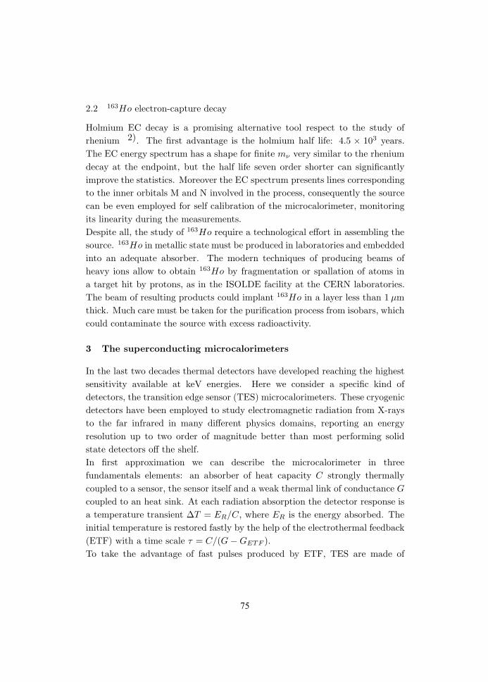
2.2 163Ho electron-capture decay

Holmium EC decay is a promising alternative tool respect to the study of

rhenium 2). The first advantage is the holmium half life: 4.5 × 103 years.

The EC energy spectrum has a shape for finite mν very similar to the rhenium

decay at the endpoint, but the half life seven order shorter can significantly

improve the statistics. Moreover the EC spectrum presents lines corresponding

to the inner orbitals M and N involved in the process, consequently the source

can be even employed for self calibration of the microcalorimeter, monitoring

its linearity during the measurements.

Despite all, the study of 163Ho require a technological effort in assembling the

source. 163Ho in metallic state must be produced in laboratories and embedded

into an adequate absorber. The modern techniques of producing beams of

heavy ions allow to obtain 163Ho by fragmentation or spallation of atoms in

a target hit by protons, as in the ISOLDE facility at the CERN laboratories.

The beam of resulting products could implant 163Ho in a layer less than 1 µm

thick. Much care must be taken for the purification process from isobars, which

could contaminate the source with excess radioactivity.

3 The superconducting microcalorimeters

In the last two decades thermal detectors have developed reaching the highest

sensitivity available at keV energies. Here we consider a specific kind of

detectors, the transition edge sensor (TES) microcalorimeters. These cryogenic

detectors have been employed to study electromagnetic radiation from X-rays

to the far infrared in many different physics domains, reporting an energy

resolution up to two order of magnitude better than most performing solid

state detectors off the shelf.

In first approximation we can describe the microcalorimeter in three

fundamentals elements: an absorber of heat capacity C strongly thermally

coupled to a sensor, the sensor itself and a weak thermal link of conductance G

coupled to an heat sink. At each radiation absorption the detector response is

a temperature transient ∆T = ER/C, where ER is the energy absorbed. The

initial temperature is restored fastly by the help of the electrothermal feedback

(ETF) with a time scale τ = C/(G − GETF ).

To take the advantage of fast pulses produced by ETF, TES are made of

75

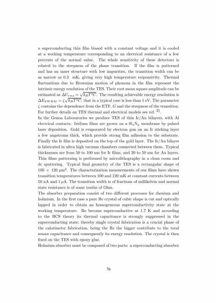
a superconducting thin film biased with a constant voltage and it is cooled

at a working temperature corresponding to an electrical resistance of a few

percents of the normal value. The whole sensitivity of these detectors is

related to the steepness of the phase transition. If the film is patterned

and has an inner structure with low impurities, the transition width can be

as narrow as 0.3 mK, giving very high temperature responsivity. Thermal

fluctuations due to Brownian motion of phonons in the film represent the

intrinsic energy resolution of the TES. Their root mean square amplitude can be

estimated as ∆Urms =√

kBT 2C. The resulting achievable energy resolution is

∆EFWHM = ζ√

kBT 2C, that in a typical case is less than 1 eV. The parameter

ζ contains the dependence from the ETF, G and the steepness of the transition.

For further details on TES thermal and electrical models see ref. 3).

In the Genoa Laboratories we produce TES of thin Ir/Au bilayers, with Al

electrical contacts. Iridium films are grown on a SixNy membrane by pulsed

laser deposition. Gold is evaporated by electron gun on an Ir sticking layer

a few angstroms thick, which provide strong film adhesion to the substrate.

Finally the Ir film is deposited on the top of the gold layer. The Ir/Au bilayer

is fabricated in ultra high vacuum chambers connected between them. Typical

thicknesses are from 50 to 100 nm for Ir films, and 20 to 50 nm for Au layers.

Thin films patterning is performed by microlithography in a clean room and

dc sputtering. Typical final geometry of the TES is a rectangular shape of

100 × 120 µm2. The characterization measurements of our films have shown

transition temperatures between 100 and 120 mK at constant currents between

50 nA and 1 µA. The transition width is of fractions of millikelvin and normal

state resistance is of some tenths of Ohm.

The absorber preparation consist of two different processes for rhenium and

holmium. In the first case a pure Re crystal of cubic shape is cut and optically

lapped in order to obtain an homogeneous superconductivity state at the

working temperature. Re become superconductive at 1.7 K and according

to the BCS theory its thermal capacitance is strongly suppressed in the

superconducting state; thereby single crystal fabrication is a crucial phase of

the calorimeter fabrication, being the Re the bigger contribute to the total

sensor capacitance and consequently its energy resolution. The crystal is then

fixed on the TES with epoxy glue.

Holmium absorber must be composed of two parts: a superconducting absorber

76

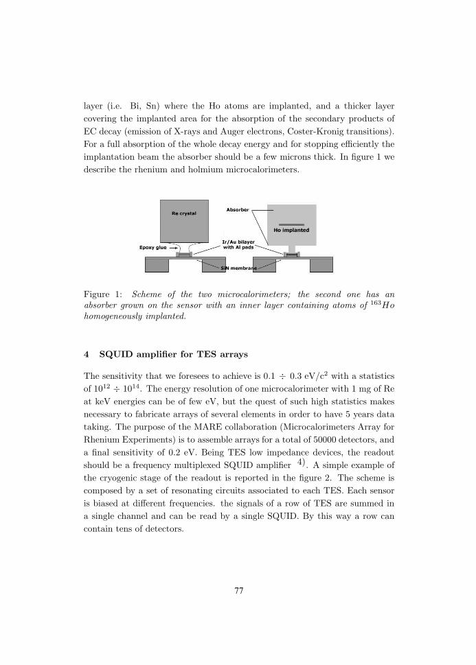
layer (i.e. Bi, Sn) where the Ho atoms are implanted, and a thicker layer

covering the implanted area for the absorption of the secondary products of

EC decay (emission of X-rays and Auger electrons, Coster-Kronig transitions).

For a full absorption of the whole decay energy and for stopping efficiently the

implantation beam the absorber should be a few microns thick. In figure 1 we

describe the rhenium and holmium microcalorimeters.

Figure 1: Scheme of the two microcalorimeters; the second one has an

absorber grown on the sensor with an inner layer containing atoms of 163Hohomogeneously implanted.

4 SQUID amplifier for TES arrays

The sensitivity that we foresees to achieve is 0.1 ÷ 0.3 eV/c2 with a statistics

of 1012 ÷ 1014. The energy resolution of one microcalorimeter with 1 mg of Re

at keV energies can be of few eV, but the quest of such high statistics makes

necessary to fabricate arrays of several elements in order to have 5 years data

taking. The purpose of the MARE collaboration (Microcalorimeters Array for

Rhenium Experiments) is to assemble arrays for a total of 50000 detectors, and

a final sensitivity of 0.2 eV. Being TES low impedance devices, the readout

should be a frequency multiplexed SQUID amplifier 4). A simple example of

the cryogenic stage of the readout is reported in the figure 2. The scheme is

composed by a set of resonating circuits associated to each TES. Each sensor

is biased at different frequencies. the signals of a row of TES are summed in

a single channel and can be read by a single SQUID. By this way a row can

contain tens of detectors.

77

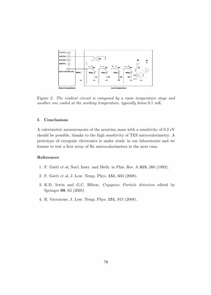
Figure 2: The readout circuit is composed by a room temperature stage and

another one cooled at the working temperature, typically below 0.1 mK.

5 Conclusions

A calorimetric measurements of the neutrino mass with a sensitivity of 0.2 eV

should be possible, thanks to the high sensitivity of TES microcalorimetry. A

prototype of cryogenic electronics is under study in our laboratories and we

foresee to test a first array of Re microcalorimeters in the next runs.

References

1. F. Gatti et al, Nucl. Instr. and Meth. in Phis. Res. A 315, 260 (1992).

2. F. Gatti et al, J. Low. Temp. Phys. 151, 603 (2008).

3. K.D. Irwin and G.C. Hilton, Cryogenic Particle detection edited by

Springer 99, 63 (2005)

4. R. Vaccarone, J. Low. Temp. Phys. 151, 915 (2008).

78

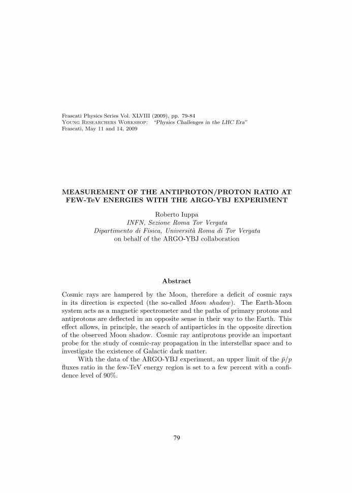
Frascati Physics Series Vol. XLVIII (2009), pp. 79-84Young Researchers Workshop: “Physics Challenges in the LHC Era”

Frascati, May 11 and 14, 2009

MEASUREMENT OF THE ANTIPROTON/PROTON RATIO ATFEW-TeV ENERGIES WITH THE ARGO-YBJ EXPERIMENT

Roberto IuppaINFN, Sezione Roma Tor Vergata

Dipartimento di Fisica, Universita Roma di Tor Vergata

on behalf of the ARGO-YBJ collaboration

Abstract

Cosmic rays are hampered by the Moon, therefore a deficit of cosmic raysin its direction is expected (the so-called Moon shadow). The Earth-Moonsystem acts as a magnetic spectrometer and the paths of primary protons andantiprotons are deflected in an opposite sense in their way to the Earth. Thiseffect allows, in principle, the search of antiparticles in the opposite directionof the observed Moon shadow. Cosmic ray antiprotons provide an importantprobe for the study of cosmic-ray propagation in the interstellar space and toinvestigate the existence of Galactic dark matter.

With the data of the ARGO-YBJ experiment, an upper limit of the p/pfluxes ratio in the few-TeV energy region is set to a few percent with a confi-dence level of 90%.

79

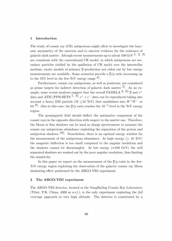
1 Introduction

The study of cosmic ray (CR) antiprotons might allow to investigate the bary-

onic asymmetry of the universe and to uncover evidence for the existence of

galactic dark matter. Altough recent measurements up to about 100 GeV 1, 2, 3)

are consistent with the conventional CR model, in which antiprotons are sec-

ondary particles yielded by the spallation of CR nuclei over the interstellar

medium, exotic models of primary p production not ruled out by low energy

measurements are available. Some scenarios provide a p/p ratio increasing up

to the 10% level in the few-TeV energy range 4).

Furthermore, cosmic ray antiprotons, as well as positrons, are considered

as prime targets for indirect detection of galactic dark matter 5). As an ex-

ample, some recent analyses suggest that the overall PAMELA 3, 6) p and e+

data and ATIC/PPB-BETS 7, 8) e+ + e− data can be reproduced taking into

account a heavy DM particle (M ≥10 TeV) that annihilates into W+W− or

hh 9). Also in this case, the p/p ratio reaches the 10−2 level in the TeV energy

region.

The geomagnetic field should deflect the antimatter component of the

cosmic rays in the opposite direction with respect to the matter one. Therefore,

the Moon or Sun shadows can be used as charge spectrometer to measure the

cosmic ray antiprotons abundance exploiting the separation of the proton and

antiproton shadows 10). Nonetheless, there is an optimal energy window for

the measurement of the antiprotons abundance. At high energy (≥ 10 TeV)

the magnetic deflection is too small compared to the angular resolution and

the shadows cannot be disentangled. At low energy (≈100 GeV) the well

separated shadows are washed out by the poor angular resolution, thus limiting

the sensitivity.

In this paper we report on the measurement of the p/p ratio in the few-

TeV energy region exploiting the observation of the galactic cosmic ray Moon

shadowing effect performed by the ARGO-YBJ experiment.

2 The ARGO-YBJ experiment

The ARGO-YBJ detector, located at the YangBaJing Cosmic Ray Laboratory

(Tibet, P.R. China, 4300 m a.s.l.), is the only experiment exploiting the full

coverage approach at very high altitude. The detector is constituted by a

80

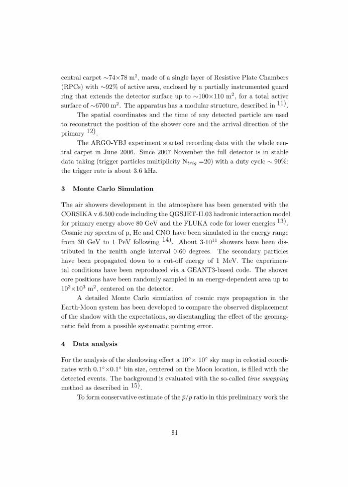
central carpet ∼74×78 m2, made of a single layer of Resistive Plate Chambers

(RPCs) with ∼92% of active area, enclosed by a partially instrumented guard

ring that extends the detector surface up to ∼100×110 m2, for a total active

surface of ∼6700 m2. The apparatus has a modular structure, described in 11).

The spatial coordinates and the time of any detected particle are used

to reconstruct the position of the shower core and the arrival direction of the

primary 12).

The ARGO-YBJ experiment started recording data with the whole cen-

tral carpet in June 2006. Since 2007 November the full detector is in stable

data taking (trigger particles multiplicity Ntrig =20) with a duty cycle ∼ 90%:

the trigger rate is about 3.6 kHz.

3 Monte Carlo Simulation

The air showers development in the atmosphere has been generated with the

CORSIKA v.6.500 code including the QGSJET-II.03 hadronic interaction model

for primary energy above 80 GeV and the FLUKA code for lower energies 13).

Cosmic ray spectra of p, He and CNO have been simulated in the energy range

from 30 GeV to 1 PeV following 14). About 3·1011 showers have been dis-

tributed in the zenith angle interval 0-60 degrees. The secondary particles

have been propagated down to a cut-off energy of 1 MeV. The experimen-

tal conditions have been reproduced via a GEANT3-based code. The shower

core positions have been randomly sampled in an energy-dependent area up to

103×103 m2, centered on the detector.

A detailed Monte Carlo simulation of cosmic rays propagation in the

Earth-Moon system has been developed to compare the observed displacement

of the shadow with the expectations, so disentangling the effect of the geomag-

netic field from a possible systematic pointing error.

4 Data analysis

For the analysis of the shadowing effect a 10× 10 sky map in celestial coordi-

nates with 0.1×0.1 bin size, centered on the Moon location, is filled with the

detected events. The background is evaluated with the so-called time swapping

method as described in 15).

To form conservative estimate of the p/p ratio in this preliminary work the

81

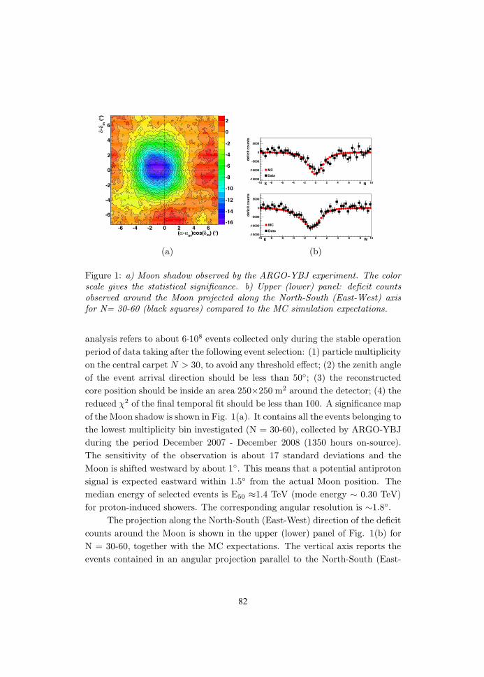
)°) (mδ)cos(mα-α(-6 -4 -2 0 2 4 6

)° (mδ-δ

-6

-4

-2

0

2

4

6

-16

-14

-12

-10

-8

-6

-4

-2

0

2

(a)

-10 -8 -6 -4 -2 0 2 4 6 8 10

def

icit

co

un

ts

-15000

-10000

-5000

0

5000

S N

MC

Data

-10 -8 -6 -4 -2 0 2 4 6 8 10

def

icit

co

un

ts

-15000

-10000

-5000

0

5000

E W

MC

Data

(b)

Figure 1: a) Moon shadow observed by the ARGO-YBJ experiment. The color

scale gives the statistical significance. b) Upper (lower) panel: deficit counts

observed around the Moon projected along the North-South (East-West) axis

for N= 30-60 (black squares) compared to the MC simulation expectations.

analysis refers to about 6·108 events collected only during the stable operation

period of data taking after the following event selection: (1) particle multiplicity

on the central carpet N > 30, to avoid any threshold effect; (2) the zenith angle

of the event arrival direction should be less than 50; (3) the reconstructed

core position should be inside an area 250×250 m2 around the detector; (4) the

reduced χ2 of the final temporal fit should be less than 100. A significance map

of the Moon shadow is shown in Fig. 1(a). It contains all the events belonging to

the lowest multiplicity bin investigated (N = 30-60), collected by ARGO-YBJ

during the period December 2007 - December 2008 (1350 hours on-source).

The sensitivity of the observation is about 17 standard deviations and the

Moon is shifted westward by about 1. This means that a potential antiproton

signal is expected eastward within 1.5 from the actual Moon position. The

median energy of selected events is E50 ≈1.4 TeV (mode energy ∼ 0.30 TeV)

for proton-induced showers. The corresponding angular resolution is ∼1.8.

The projection along the North-South (East-West) direction of the deficit

counts around the Moon is shown in the upper (lower) panel of Fig. 1(b) for

N = 30-60, together with the MC expectations. The vertical axis reports the

events contained in an angular projection parallel to the North-South (East-

82

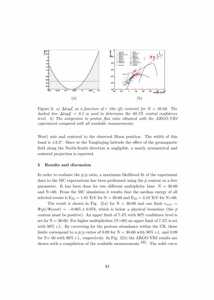
r-0.2 -0.15 -0.1 -0.05 0 0.05 0.1

log

L∆-

0

0.2

0.4

0.6

0.8

1

1.2

1.4

1.6

1.8

2

2.2

2.4

(a)

energy (GeV)-210 -110 1 10 210 310 410 510

/p r

atio

p

-610

-510

-410

-310

-210

-110

1Golden 79 BSP 81Golden 84 Stephens 85Bogomolov 87-90 LEAP 90PBAR 90 MASS 91IMAX 95 BESS 95-97Caprice 97 CAPRICE 98HEAT 01 L3+ 03MACRO 05 07γTibet-ASPAMELA 09 Argo 09 - 90% C.L.

Shibata 08Stecker 85 Cirelli 09

(b)

Figure 2: a) ∆logL as a function of r (the (p) content) for N = 30-60. The

dashed line ∆logL = 0.5 is used to determine the 68.3% central confidence

level. b) The antiproton to proton flux ratio obtained with the ARGO-YBJ

experiment compared with all available measurements.

West) axis and centered to the observed Moon position. The width of this

band is ±3.3. Since at the Yangbajing latitude the effect of the geomagnetic

field along the North-South direction is negligible, a nearly symmetrical and

centered projection is expected.

5 Results and discussion

In order to evaluate the p/p ratio, a maximum likelihood fit of the experiment

data to the MC expectations has been performed using the p content as a free

parameter. It has been done for two different multiplicity bins: N = 30-60

and N>60. From the MC simulation it results that the median energy of all

selected events is E50 = 1.85 TeV for N = 30-60 and E50 = 4.10 TeV for N>60.

The result is shown in Fig. 2(a) for N = 30-60 and one finds rmin =

Φ(p)/Φ(mat) = −0.065 ± 0.078, which is below a physical boundary (the p

content must be positive). An upper limit of 7.4% with 90% confidence level is

set for N = 30-60. For higher multiplicities (N>60) an upper limit of 7.4% is set

with 90% c.l.. By correcting for the protons abundance within the CR, these

limits correspond to a p/p ratios of 0.09 for N = 30-60 with 90% c.l. and 0.09

for N> 60 with 90% c.l., respectively. In Fig. 2(b) the ARGO-YBJ results are

shown with a compilation of the available measurements 16). The solid curve

83

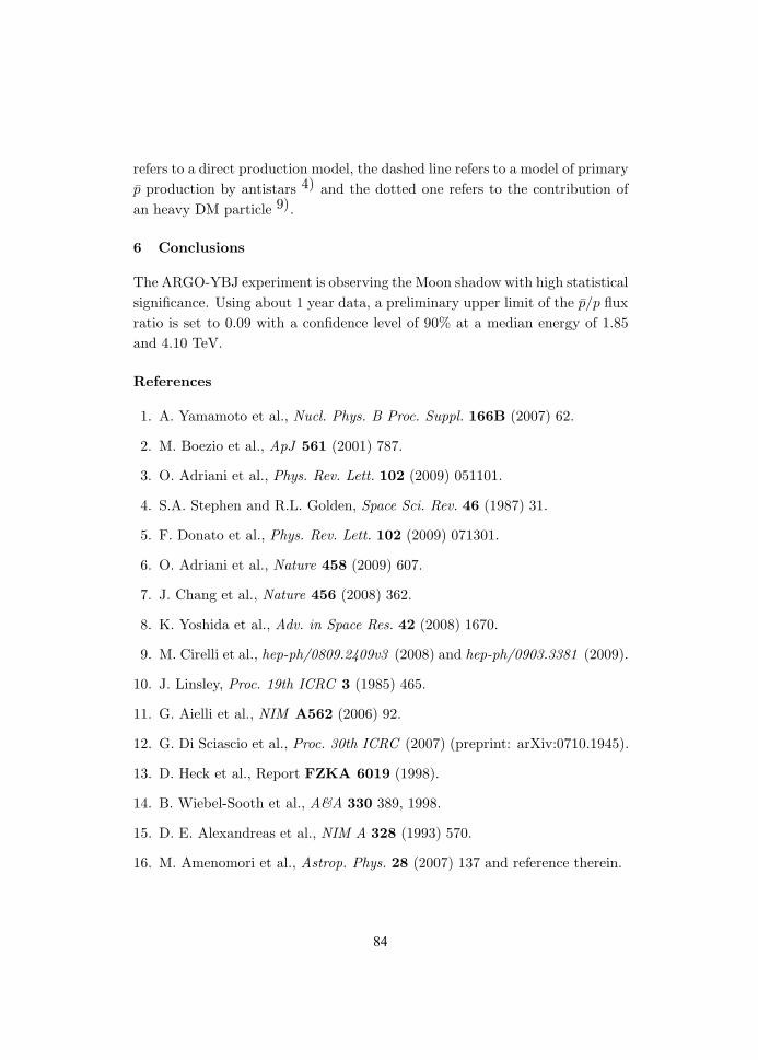
refers to a direct production model, the dashed line refers to a model of primary

p production by antistars 4) and the dotted one refers to the contribution of

an heavy DM particle 9).

6 Conclusions

The ARGO-YBJ experiment is observing the Moon shadow with high statistical

significance. Using about 1 year data, a preliminary upper limit of the p/p flux

ratio is set to 0.09 with a confidence level of 90% at a median energy of 1.85

and 4.10 TeV.

References

1. A. Yamamoto et al., Nucl. Phys. B Proc. Suppl. 166B (2007) 62.

2. M. Boezio et al., ApJ 561 (2001) 787.

3. O. Adriani et al., Phys. Rev. Lett. 102 (2009) 051101.

4. S.A. Stephen and R.L. Golden, Space Sci. Rev. 46 (1987) 31.

5. F. Donato et al., Phys. Rev. Lett. 102 (2009) 071301.

6. O. Adriani et al., Nature 458 (2009) 607.

7. J. Chang et al., Nature 456 (2008) 362.

8. K. Yoshida et al., Adv. in Space Res. 42 (2008) 1670.

9. M. Cirelli et al., hep-ph/0809.2409v3 (2008) and hep-ph/0903.3381 (2009).

10. J. Linsley, Proc. 19th ICRC 3 (1985) 465.

11. G. Aielli et al., NIM A562 (2006) 92.

12. G. Di Sciascio et al., Proc. 30th ICRC (2007) (preprint: arXiv:0710.1945).

13. D. Heck et al., Report FZKA 6019 (1998).

14. B. Wiebel-Sooth et al., A&A 330 389, 1998.

15. D. E. Alexandreas et al., NIM A 328 (1993) 570.

16. M. Amenomori et al., Astrop. Phys. 28 (2007) 137 and reference therein.

84

Frascati Physics Series Vol. XLVIII (2009), pp. 85-90Young Researchers Workshop: “Physics Challenges in the LHC Era”

Frascati, May 11 and 14, 2009

EVENT RECONSTRUCTION IN THE DRIFT CHAMBER OFTHE CMD-3 DETECTOR

A.V. Karavdina∗

Budker Institute of Nuclear Physics, Novosibirsk, Russia

Abstract

Charged particles tracks and vertex reconstruction as well as offline-calibrationsin the drift chamber of the CMD-3 detector are described. Event reconstructionalgoritm was tested on simulation in the magnetic field. Spatial resolution90÷120 µm in the drift plane and 1.5÷3 mm along wires were obtained in testexperiments without the magnetic field.

1 Introduction

The new electron-positron collider VEPP-2000 1) is being now under commis-

sioning at Budker Institute of Nuclear Physics. Using round beams technique

the collider will provide the luminosity up to 1032 cm−2s−1 at the maximum

∗On behalf of the CMD-3 Collaboration

85

c.m. energy√

s = 2 GeV. Main goals of experiments at the VEPP-2000 are

studies interaction of light quarks produced in e+e− collisions, test of exist-

ing theoretical and phenomenological models and provide precise information

for future models. It requires a detector with high efficiency for multypartice

events and good energy and angular resolutions for charged particles as well as

for photons.

Two modern detectors, a general purpose detector CMD-3 (Cryogenic

Magnetic Detector) and SND (Spherical Neutral Detector), will be installed in

the two interaction regions of the collider. The CMD-3 detector consists of a

cylindrical drift chamber and Z-chamber inside thin (0.18X0) superconductive

solenoid with the 1.35 T magnetic field, end-cap BGO calorimeter, barrel liquid

xenon and CsI calorimeters, TOF counters between LXe and CsI calorimeters

and cosmic veto counters. In more detail the CMD-3 detector is described

elsewhere 2).

2 Drift chamber

The drift chamber is a cylinder of 44 cm length and 60(4) cm outer(inner)

diameter. The sensitive volume of the drift chamber is filled by 1218 identi-

cal hexagonal drift cells. The cell side length is 9 mm. Each sense wire is

surrounded by 6 field wires. Charge division technique is used to measure co-

ordinate along sense wires which have 15 µm diameter and are made of gold

plated tungsten-rhenium alloy with resistance of 1 kΩ/m. Field wires have 100

µm diameter and are made of titanium. The drift chamber is filled with a 80:20

mixture of argon and isobutane. In more detail the drift chamber construction

is discussed elsewhere 3).

The digitized measurements of time and two charges from the ends of

sense wires are provided by T2Q boards that were produced at the Institute

workshop. Analog and digital parts of it are placed on one board. The board

is made in BigCAMAC standard and serves 16 sense wires.

3 Track reconstruction

Direct measurements of the magnetic field in the drift chamber volume have

shown good agreement with calculations. The maximum deviation of the z-

component of the magnetic field does not exceed 1% along the beam axis and

86

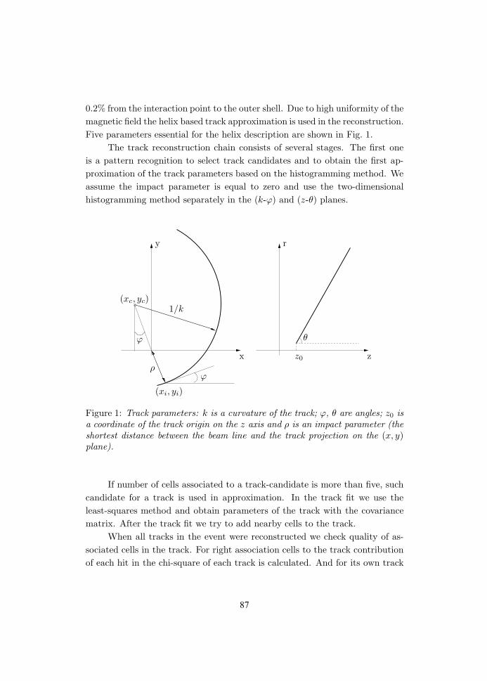
0.2% from the interaction point to the outer shell. Due to high uniformity of the

magnetic field the helix based track approximation is used in the reconstruction.

Five parameters essential for the helix description are shown in Fig. 1.

The track reconstruction chain consists of several stages. The first one

is a pattern recognition to select track candidates and to obtain the first ap-

proximation of the track parameters based on the histogramming method. We

assume the impact parameter is equal to zero and use the two-dimensional

histogramming method separately in the (k-ϕ) and (z-θ) planes.

x

y

1/k

ϕ

ϕρ

(xc, yc)

(xi, yi)

r

zz0

θ

Figure 1: Track parameters: k is a curvature of the track; ϕ, θ are angles; z0 is

a coordinate of the track origin on the z axis and ρ is an impact parameter (the

shortest distance between the beam line and the track projection on the (x, y)plane).

If number of cells associated to a track-candidate is more than five, such

candidate for a track is used in approximation. In the track fit we use the

least-squares method and obtain parameters of the track with the covariance

matrix. After the track fit we try to add nearby cells to the track.

When all tracks in the event were reconstructed we check quality of as-

sociated cells in the track. For right association cells to the track contribution

of each hit in the chi-square of each track is calculated. And for its own track

87

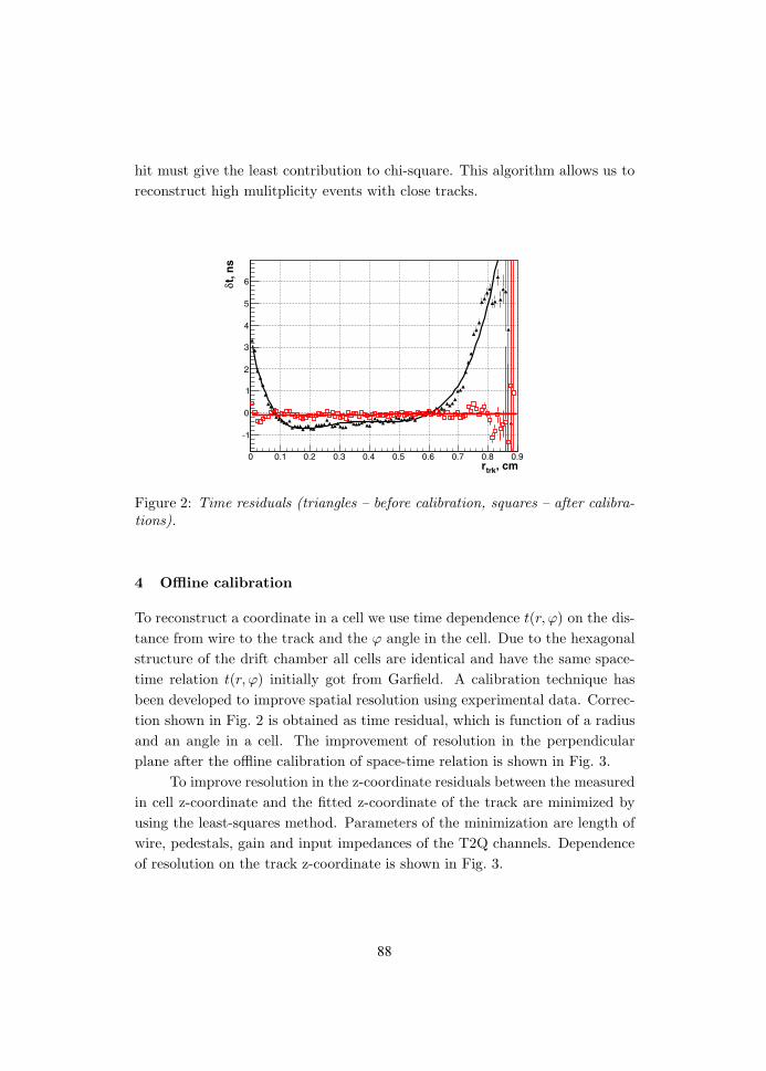
hit must give the least contribution to chi-square. This algorithm allows us to

reconstruct high mulitplicity events with close tracks.

, cmtrkr0 0.1 0.2 0.3 0.4 0.5 0.6 0.7 0.8 0.9

t, n

sδ

-1

0

1

2

3

4

5

6

Figure 2: Time residuals (triangles – before calibration, squares – after calibra-

tions).

4 Offline calibration

To reconstruct a coordinate in a cell we use time dependence t(r, ϕ) on the dis-

tance from wire to the track and the ϕ angle in the cell. Due to the hexagonal

structure of the drift chamber all cells are identical and have the same space-

time relation t(r, ϕ) initially got from Garfield. A calibration technique has

been developed to improve spatial resolution using experimental data. Correc-

tion shown in Fig. 2 is obtained as time residual, which is function of a radius

and an angle in a cell. The improvement of resolution in the perpendicular

plane after the offline calibration of space-time relation is shown in Fig. 3.

To improve resolution in the z-coordinate residuals between the measured

in cell z-coordinate and the fitted z-coordinate of the track are minimized by

using the least-squares method. Parameters of the minimization are length of

wire, pedestals, gain and input impedances of the T2Q channels. Dependence

of resolution on the track z-coordinate is shown in Fig. 3.

88

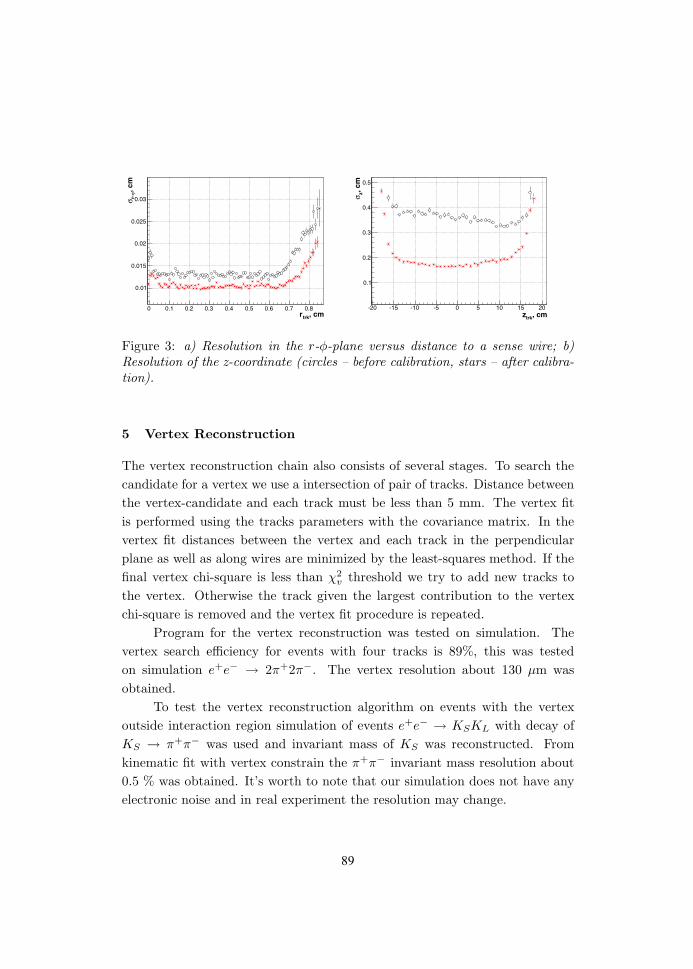
, cmtrkr0 0.1 0.2 0.3 0.4 0.5 0.6 0.7 0.8

, cm

ϕr-σ

0.01

0.015

0.02

0.025

0.03

, cmtrkz-20 -15 -10 -5 0 5 10 15 20

, cm

zσ

0.1

0.2

0.3

0.4

0.5

Figure 3: a) Resolution in the r-φ-plane versus distance to a sense wire; b)

Resolution of the z-coordinate (circles – before calibration, stars – after calibra-

tion).

5 Vertex Reconstruction

The vertex reconstruction chain also consists of several stages. To search the

candidate for a vertex we use a intersection of pair of tracks. Distance between

the vertex-candidate and each track must be less than 5 mm. The vertex fit

is performed using the tracks parameters with the covariance matrix. In the

vertex fit distances between the vertex and each track in the perpendicular

plane as well as along wires are minimized by the least-squares method. If the

final vertex chi-square is less than χ2v threshold we try to add new tracks to

the vertex. Otherwise the track given the largest contribution to the vertex

chi-square is removed and the vertex fit procedure is repeated.

Program for the vertex reconstruction was tested on simulation. The

vertex search efficiency for events with four tracks is 89%, this was tested

on simulation e+e− → 2π+2π−. The vertex resolution about 130 µm was

obtained.

To test the vertex reconstruction algorithm on events with the vertex

outside interaction region simulation of events e+e− → KSKL with decay of

KS → π+π− was used and invariant mass of KS was reconstructed. From

kinematic fit with vertex constrain the π+π− invariant mass resolution about

0.5 % was obtained. It’s worth to note that our simulation does not have any

electronic noise and in real experiment the resolution may change.

89

6 Conclusion

Event reconstruction in the drift chamber of the CMD-3 detector is imple-

mented. This software includes reconstruction of charged particles tracks, ver-

tices and several offline calibrations. The algorithm of the track reconstruction

and the offline calibrations were tested on the experimental data without the

magnetic field as well as on simulation in presence of the magnetic field. The

experimental resolution 90÷120 µm in the perpendicular plane and 1.5÷3 mm

along wires was reached. The vertex reconstruction was tested on non-central

(KS → π+π−) and central (e+e− → 2π+2π−) simulated events in the magnetic

field.

Test of the event reconstruction efficiency are still in progress. Also we

plan to use the Kalman filter for low-energy particle track reconstruction. This

method allows us taking into account multiple scattering in the track fit, which

is necessary for charged kaons at the threshold.

References

1. Yu.M. Shatunov et al., Proc. of EPAC 2000, 439 (Vienna, Austria, 2000).

2. G.V. Fedotovich, Nucl. Phys. B162, 332 (2006).

3. A. Popov et al., Nucl. Instr. and Meth. A598, 105 (2009).

90

Frascati Physics Series Vol. XLVIII (2009), pp. 91Young Researchers Workshop: “Physics Challenges in the LHC Era”

Frascati, May 11 and 14, 2009

KAONIC ATOMS AT DAΦNE

Shinji OkadaLaboratori Nazionali di Frascati dell’INFN,

Via Enrico Fermi 40, 00044 Frascati, Italy

Written contribution not received

91

92

FRASCATI PHYSICS SERIES VOLUMES

Volume IHeavy Quarks at Fixed Target

Eds.: S. Bianco and F.L. FabbriFrascati, May 31–June 2, 1993ISBN—88–86409–00–1

Volume II – Special IssueLes Rencontres de Physique de la Vallee d’Aoste –

Results and Perspectives in Particle Physics

Ed.: M. GrecoLa Thuile, Aosta Valley, March 5 –11, 1995ISBN—88–86409–03–6

Volume IIIHeavy Quarks at Fixed Target

Ed.: B. CoxUniversity of Virginia, CharlottesvilleOctober 7–10, 1994, 11ISBN—88–86409–04–4

Volume IVWorkshop on Physics and Detectors for DAΦNE

Eds.: R. Baldini, F. Bossi, G. Capon, G. PancheriFrascati, April 4–7, 1995ISBN—88–86409–05–2

Volume V – Special IssueLes Rencontres de Physique de la Vallee d’Aoste –

Results and Perspectives in Particle Physics

Ed.: M. GrecoLa Thuile, Aosta Valley, March 3–9, 1996ISBN—88–86409–07–9

Volume VICalorimetry in High Energy Physics

Eds.: A. Antonelli, S. Bianco, A. Calcaterra, F.L. FabbriFrascati, June 8–14, 1996ISBN—88–86409–10–9

93

Volume VIIHeavy Quarks at Fixed Target

Ed.: L. KopkeRhinefels Castle, St. Goar, October 3–6, 1996ISBN—88–86409–11–7

Volume VIIIADONE a milestone on the particle way

Ed.: V. Valente 1997ISBN—88–86409–12–5

Volume IX – Special IssueLes Rencontres de Physique de la Vallee d’Aoste –

Results and Perspectives in Particle Physics

Ed.: M. GrecoLa Thuile, Aosta Valley, March 2–8, 1997ISBN–88–86409–13–3

Volume XAdvanced ICFA Beam Dynamics

Workshop on Beam Dynamics Issue for e+e− Factories

Eds.: L. Palumbo, G. VignolaFrascati, October 20–25, 1997ISBN—88–86409–14–1

Volume XIProceedings of the XVIII International Conference on

Physics in Collision

Eds.: S. Bianco, A. Calcaterra, P. De Simone, F. L. FabbriFrascati, June 17–19, 1998ISBN—88–86409–15–X

Volume XII – Special IssueLes Rencontres de Physique de la Vallee d’Aoste –

Results and Perspectives in Particle Physics

Ed.: M. GrecoLa Thuile, Aosta Valley, March 1–7, 1998ISBN—88–86409–16–8

94

Volume XIIIBruno Touschek and the Birth of thee+e−

Ed.: G. IsidoriFrascati, 16 November, 1998ISBN—88–86409–17–6

Volume XIV – Special IssueLes Rencontres de Physique de la Vallee d’Aoste –

Results and Perspectives in Particle Physics

Ed.: M. GrecoLa Thuile, Aosta Valley, February 28–March 6, 1999ISBN—88–86409–18–4

Volume XVWorkshop on Hadron Spectroscopy

Eds.: T. Bressani, A. Feliciello, A. FilippiFrascati, March 8 2 1999ISBN—88–86409–19–2

Volume XVIPhysics and Detectors for DAΦNE

Eds.: S. Bianco, F. Bossi, G. Capon, F.L. Fabbri,P. Gianotti, G. Isidori, F. MurtasFrascati, November 16 –19, 1999ISBN—88–86409–21–4

Volume XVII – Special IssueLes Rencontres de Physique de la Vallee d’Aoste –

Results and Perspectives in Particle Physics

Ed.: M. GrecoLa Thuile, Aosta Valley, February 27 March 4, 2000ISBN—88–86409–23–0

Volume XVIIILNF Spring School

Ed.: G. PancheriFrascati 15–20 May, 2000ISBN—88–86409–24–9

95

Volume XIXXX Physics in Collision

Ed.: G. BarreiraLisbon June 29–July1st. 2000ISBN—88–86409–25–7

Volume XXHeavy Quarks at Fixed Target

Eds.: I. Bediaga, J. Miranda, A. ReisRio de Janeiro, Brasil, October 9–12, 2000ISBN—88–86409–26–5

Volume XXIIX International Conference on Calorimetry in

High Energy Physics

Eds.: B. Aubert, J. Colas, P. Nedelec, L. PoggioliAnnecy Le Vieux Cedex, France, October 9–14, 2000ISBN—88–86409–27–3

Volume XXII – Special IssueLes Rencontres de Physique de la Vallee d’Aoste –

Results and Perspectives in Particle Physics

Ed.: M. GrecoLa Thuile, Aosta Valley, March 4–10, 2001ISBN—88–86409–28–1

Volume XXIIIXXI Physics in Collision

Ed.: Soo–Bong KimSeoul, Korea, June 28 30, 2001ISBN—88–86409–30–3

Volume XXIVInternational School of Space Science – 2001 Course on:

Astroparticle and Gamma–ray Physics in Space

Eds.: A. Morselli, P. PicozzaL’Aquila, Italy, August 30 September 7, 2000ISBN—88–86409–31–1

96

Volume XXVTRDs for the 3rd Millennium Workshop on

Advanced Transition Radiation Detectors for

Accelerator and Space Applications

Eds. N. Giglietto, P. SpinelliBari, Italy, September 20–23, 2001ISBN—88–86409–32–X

Volume XXVIKAON 2001 International Conference on CP ViolationEds.: F. Costantini, G. Isidori, M. SozziPisa Italy, June 12th 17th, 2001ISBN—88–86409–33–8

Volume XXVII – Special IssueLes Rencontres de Physique de la Vallee d’Aoste –

Results and Perspectives in Particle Physics

Ed.: M. GrecoLa Thuile, Aosta Valley, March 3–9, 2002ISBN—88–86409–34–6

Volume XXVIIIHeavy Quarks at Leptons 2002

Eds.: G. Cataldi, F. Grancagnolo, R. Perrino, S. SpagnoloVietri sul mare (Italy), May 27th June 1st, 2002ISBN—88–86409–35–4

Volume XXIXWorkshop on Radiation Dosimetry: Basic Technologies,

Medical Applications, Environmental Applications

Ed.: A. ZaniniRome (Italy), February 56, 2002ISBN—88–86409–36–2

Volume XXIX – Suppl.Workshop on Radiation Dosimetry: Basic Technologies,

Medical Applications, Environmental Applications

Ed.: A. ZaniniRome (Italy), February 56, 2002ISBN—88–86409–36–2

97

Volume XXX – Special IssueLes Rencontres de Physique de la Vallee d’Aoste –

Results and Perspectives in Particle Physics

Ed.: M. GrecoLa Thuile, Aosta Valley, March 9–15, 2003ISBN—88–86409–39–9

Volume XXXIFrontier Science 2002 – Charm, Beauty and CP,

First International Workshop on Frontier Science

Eds.: L. Benussi, R. de Sangro, F.L. Fabbri, P. ValenteFrascati, October 6–11, 2002ISBN—88–86409–37–0

Volume XXXII19th International Conference on x–ray and Inner–Shell Processes

Eds.: A. Bianconi, A. Marcelli, N.L. SainiUniversita di Roma La Sapienza June 24–28, 2002ISBN—88–86409–39–07

Volume XXXIIIBruno Touschek Memorial Lectures

Ed.: M. Greco, G. PancheriFrascati, May 11, 1987ISBN—88–86409–40–0

Volume XXXIV – Special IssueLes Rencontres de Physique de la Vallee d’Aoste –

Results and Perspectives in Particle Physics

Ed.: M. GrecoLa Thuile, Aosta Valley, February 29 – March 6, 2004ISBN—88–86409–42–7

Volume XXXVHeavy Quarks And Leptons 2004

Ed.: A. LopezSan Juan, Puerto Rico, 1–5 June 2004ISBN—88–86409–43–5

98

Volume XXXVIDAΦNE 2004: Physics At Meson Factories

Eds.: F. Anulli, M. Bertani, G. Capon, C. Curceanu–Petrascu,F.L. Fabbri, S. MiscettiFrascati, June 7–11, 2004ISBN—88–86409–53–2

Volume XXXVIIFrontier Science 2004, Physics and Astrophysics in Space

Eds.: A. Morselli, P. Picozza, M. RicciFrascati, 14–19 June, 2004ISBN—88–86409–52–4

Volume XXXVIIIII Workshop Italiano sulla Fisica di ATLAS e CMS

Eds.: Gianpaolo Carlino and Pierluigi PaolucciNapoli, October 13 – 15, 2004ISBN—88–86409–44–3

Volume XXXIX – Special IssueLes Rencontres de Physique de la Vallee d’Aoste –

Results and Perspectives in Particle Physics

Ed.: M. GrecoLa Thuile, Aosta Valley, February 27 – March 5, 2005ISBN—88–86409–45–1

Volume XLFrontier Science 2005 – New Frontiers in Subnuclear Physics

Eds.: A. Pullia, M. PaganoniMilano, September 12 - 17, 2005ISBN—88–86409–46–X

Volume XLIDiscoveries in Flavour Physics at e+e− Colliders

Eds.: L. Benussi, S. Bianco, C. Bloise, R. de Sangro, C. Gatti,G. Isidori, M. Martini, F. Mescia, S. MiscettiFrascati, February 28th - March 3rd, 2006ISBN—88–86409–51–6

99

Volume XLII – Special IssueLes Rencontres de Physique de la Vallee d’Aoste –

Results and Perspectives in Particle Physics

Ed.: M. GrecoLa Thuile, Aosta Valley, March 5 March 11, 2006ISBN—88–86409–47–8

Volume XLIII – Special IssueNeutral Kaon Interferometry at A Phi-Factory: from Quantum Mechanics to

Quantum Gravity

Ed.: A. Di DomenicoFrascati, March 24th 2006ISBN 978—88–86409–50–8

Volume XLIV– Special IssueLes Rencontres de Physique de la Vallee d’Aoste –

Results and Perspectives in Particle Physics

Ed.: M. GrecoLa Thuile, Aosta Valley, February 28, 2 March 5, 2007ISBN 978—88–86409–49–4

Volume XLV Frontier Science – Science with the New Generation

High Energy Gamma-ray Experiments

Eds.: A. Lionetto, A. MorselliVilla Mondragone, Monteporzio, Italy June 18 -20, 2007ISBN–978—88–86409–54–0

Volume XLVIXII International Conference on Hadron Spectroscopy

Eds.: L. Benussi, M. Bertani, S. Bianco, C. Bloise, R. de Sangro, P. de Simone,P. di Nezza, P. Giannotti, S. Giovanella, M.P. Lombardo, S. PacettiLaboratori Nazionali di Frascati, October 713, 2007ISBN—978–88–86409–55–1

Volume XLVII – Special IssueLes Rencontres de Physique de la Vallee d’Aoste –

Results and Perspectives in Particle Physics

Ed.: M. GrecoLa Thuile, Aosta Valley, February 24, 2 March 1st, 2008ISBN 978–88–86409–56–8

100