IEG Working Paper No. 314 2012

Sanhita Sucharita

Institute of Economic GrowthUniversity Enclave, University of DelhiDelhi 110007, IndiaTel: 27667101/288/424; Fax: 27667410Website: www.iegindia.org

Fiscal Consolidation in India

rEcEnT WorkInG papErs

Title author (s) name paper no.

Drivers of Agricultural Diversification in india, Haryana and the Greenbelt Farms of India

Brajesh JhaAmarnath Tripathi Biswajit Mohanty

E/303/2009

Regional Openness, Income Growth and Disparity Across Major Indian States during 1980-2004

Dibyendu MaitiSugata Marjit

E/304/2010

Rethinking Agricultural Production Collectivities: The Case for a Group approach to Energize Agriculture and Empower Poor Farmers

Bina Agarwal E/305/2010

Skills, Informality and Development

Arup MitraDibyendu Maiti

E/306/2010

Club-Convergence and Polarisation of Sates: A Nonparametric Analysis of Post-Reform India

Sabyasachi KarDebajit JhaAlpana Kateja

E/307/2010

Business Group Ownership of Banks: Issues and Implications

Ashis Taru Deb E/308/2010

Does Participatory Development Legitimise Collusion echanisms? Evidence from Karnataka Watershed Development Agency

G. Ananda Vadivelu E/309/2011

Policies for Increasing Non-farm Employment for Farm Households in India

Brajesh Jha E/310/2011

Nagaland’s Demographic Somersault

Ankush Agrawal Vikas Kumar

E/311/2012

Does Access to Secondary Education Affect Primary Schooling? Evidence from India

Abhiroop MukhopadhyaySoham Sahoo

E/312/2012

Reexamining the Finance–Growth Relationship for a Developing Economy: A time series analysis of post–reform India

Sabyasachi KarKumarjit Mandal

E/313/2012

i

Fiscal Consolidation in India

Sanhita Sucharita

IEG Working Paper No. 314 2012

Sanhita Sucharita is Assistant Professor, Central University of Jharkhand, Ranchi. Email: sanhita.sucharita@gmail.com

ACKNOWLEDGEMENTS

The author is grateful to Bina Agarwal, Arup Mitra, Basanta Kumar Pradhan, JVM Sarma, Durairaj Kumarasamy, Vikram Dayal, Zakir Husain, Prakashan Chellattan Veettil, T Adi Bhawani, Purnamita Dasgupta, Sabyasachi Kar, Pravakar Sahoo, Ankush Agrawal, Swadhin Kumar Mondal, Bishwanath Goldar, Yashobanta Parida, Parul Baghel, Surit Das and Narayan Sethi for their helpful suggestion and comments. The author is also grateful to Sir Ratan Tata Trust and the Institute of Economic Growth, where this work was done during her Sir Ratan Tata fellowship tenure. All opinions expressed are personal.

Fiscal Consolidation in India

ABSTRACT

After the global economic crisis, the fiscal situation of central and state governments in India has worsened and fiscal sustainability—threatened by high deficit, unproductive expenditure, and tax distortion—has become questionable. This study attempts to understand the rationale of fiscal adjustment from the mainstream and political economy approaches. This paper examines the crowding-out effects of fiscal imbalance in India. It also attempts to understand the effect of elections on the fiscal imbalance in India. An OLS method is used to examine whether there is electoral motive towards rising fiscal deficit. The econometric investigation covers the period between 1980–81 and 2008–09. The impact of election year on the fiscal deficit-to-GDP ratio is examined by regressing gross fiscal deficit (combined government) to GDP ratio against growth rate, population growth, and elections. Towards the end, the study analyses the effectiveness of government effort to control fiscal imbalances. Empirical finding shows that there is a crowding-out effect of public investment on private investment and that elections do not significantly affect the fiscal deficit in India.

Keywords: Fiscal adjustment, crowding out, fiscal responsibility, Budget Management Act

JEL codes: H30, H40

3

1. INTRODUCTION

The growing interest in fiscal adjustment in India is attributable in part to the deterioration in its fiscal performance. India witnessed tremendous economic growth in the past two decades. Its GDP growth rate was 8 per cent but its sustainability has been in question, first with the 1991 fiscal Balance of Payments (BoP) crisis and then again after 1997–98 when fiscal deficits returned to the 10-per-cent-of-GDP range and government debt grew. Now, fiscal sustainability is in question again after the global economic crisis. To make this economic growth sustainable with macroeconomic stability, fiscal policy is a critical component. Fiscal adjustment is moderated by some attempts to reverse this trend. High deficits, unproductive expenditure, and tax distortions have constrained the economy from realising its full growth potential. The fiscal position of both central and state governments worsened significantly since the fiscal consolidation achieved after the 1991 BoP crisis. There is remarkable downward inflexibility demonstrated by the fiscal deficit and stubborn upward movement exhibited by revenue and primary deficits.

The combined fiscal deficit of the Centre and the states, which was 9.3 per cent of GDP in the crisis year of 1990–91, dropped to 6.3 per cent in 1996–97 before creeping back up to 9 per cent in 1998–99. The fiscal deficit remained at over 9 per cent until 2002–03 and has since been on a downward shift, declining to 4.2 per cent in 2007–08. Due to the global economic crisis, the fiscal deficit increased in 2009–10 to 9.3 per cent. Similarly, the combined revenue deficit of the Centre and the states, which was 4.2 per cent in the crisis year of 1990–91 and declined to 3.2 per cent by 1992–93, grew to the alarming level of 6.9 per cent by 2001–02. Like the fiscal deficit, the revenue deficit too showed a welcome downward shift since 2002–03, declining to 0.2 per cent in 2007–08. Due to the global economic crisis, it again went up to 5.7 per cent in 2009–10.

More revenue deficit implies the preemption of private saving for current government consumption, which tends to crowd out private investment without increasing the government’s capital spending correspondingly. It is also recognised that the primary deficit has turned negative since the 1990s, implying that the government is borrowing to meet their current expenditure or that a significant part of the fiscal deficit is due to the burden of serving past debt, and may create a situation of debt unsustainability. Obviously, not only the growing deficit but also its composition and the way it is being financed deserve concern because the impact of the fiscal deficit depends on it.

A loose fiscal policy in India may lead to inflation, crowding out, and debt unsustainability, which may ultimately hamper economic growth. When a loose fiscal policy tries to finance its deficit by printing money, inflation can occur. When a government

4

borrows to finance a looser fiscal position, the greater demand for loanable funds can reduce private investment by raising interest rates. Under a floating exchange rate, a higher interest rate tends to attract foreign capital, leading to an appreciation of the exchange rate, which also crowds out exports.

In India, a loose fiscal policy is financed by public borrowing and may crowd out private investment and cause debt unsustainability. The present study tries to find out the rationale of fiscal adjustment and constraints on fiscal adjustment. The present paper consists of six sections, including the introduction. Section 2 describes the mainstream perspective of or rationale for fiscal adjustment and empirically examines the crowding-out effect of real public investment on real private investment. Section 3 emphasises the rationale of fiscal adjustment from the political economy perspective and examines the effect of elections on fiscal imbalance. Section 4 evaluates different fiscal adjustment programmes and analyses their success and limitation. Section 5 concludes and summarises the study.

2. MAINSTREAM ThEORETICAL PERSPECTIvES Of RATIONALE Of fISCAL ADjUSTMENT

While the views of economists differ, debt and its increment, i.e. fiscal deficit, become unsustainable in some circumstances. There are three theoretical perspectives: neoclassical, Ricardian, and Keynesian. Depending on the circumstances and the relevant theoretical perspectives, fiscal deficit may be bad, indifferent, or good.

The neoclassical view: The neoclassical literature highlights the adverse impact of unsustainable debt and deficits. In the neoclassical perspective, a fiscal deficit will have a detrimental effect on growth if the reduction in government saving or an increase in government dissaving, which is equivalent to revenue deficit, is not fully offset by a rise in private saving. Besides affecting the overall saving rate, when there is a net fall in the saving rate, there will be pressure on the interest rate, which may crowd out private investment and therefore adversely affect growth. In this paradigm, fiscal deficits raise lifetime consumption by shifting taxes to future generations. If economic resources are fully employed, increased consumption implies decreased saving in a closed economy. In an open economy, real interest rates and investment may remain unaffected, but the fall in national saving is financed by higher external borrowing accompanied by an appreciation of the domestic currency and fall in exports. In both cases, net national saving falls and consumption rises accompanied by some combination of fall in investment and exports.

5

Keynesian view of fiscal deficit: In the mainstream fiscal literature, Keynesians give a strong argument for a high level of fiscal deficit in relation to GDP: if financed by borrowing, an increase in autonomous government expenditure—whether investment or consumption—would cause output to expand through a multiplier process particularly when there are unemployed resources. The traditional Keynesian framework does not distinguish between alternative uses of a fiscal deficit (such as between government consumption and investment expenditure) or between monetisation or external or internal borrowing as sources of financing a fiscal deficit. Although there is no explicit budget constraint in Keynes’ analysis, subsequent developments that do incorporate the budget constraint show that some Keynesian conclusions are weakened as a result. Subsequent elaboration of the Keynesian paradigms envisages that the multiplier-based expansion of output leads to a rise in the demand for money, and if money supply is fixed and the deficit is bond-financed, the interest rate would rise partially, offsetting the multiplier effect. However, Keynesians argue that increased aggregate demand enhances private investment and leads to higher investment at any given rate of interest. The effect of a rise in the interest rate may thus be more neutralised by the increased profitability of investment. Keynesians argue that deficits may stimulate saving and investment even if the interest rate rises, primarily because of the employment of unutilised resources. However, at full employment, a deficit would crowd out investment even in the Keynesian paradigm.

Ricardian equivalence perspective: In Ricardian equivalence, fiscal deficits are considered neutral in terms of their impact on growth. Financing budgets by deficits amounts only to the postponement of taxes. The deficit in any current period is exactly equal to the present value of future taxation required to pay off the increment to debt resulting from deficit.

Empirical analysis on crowding out: Here, a Vector Error Correction Model (VECM) has been used to find the crowding-out effect of public investment on private investment. The model, which captures both the long-run equilibrium between the variables and the short-run relation, used annual data from 1950 to 2008 on public investment, private investment, and GDP at factor cost (Handbook of Statistics, RBI). Here, capital formation, households, and the private corporate sector are added to obtain private investment. All the variables are defined in real terms to avoid the price effect. The GDP deflator has been used to convert the nominal data into real terms. All the variables are expressed in their natural logarithm value.

The variables were tested for stationarity and cointegration before the VECM was used. We have used both the Augmented Dickey-Fuller (ADF) and the Phillips-Perron (PP) unit root tests to determine the order of integration of the variables (Table 1).

6

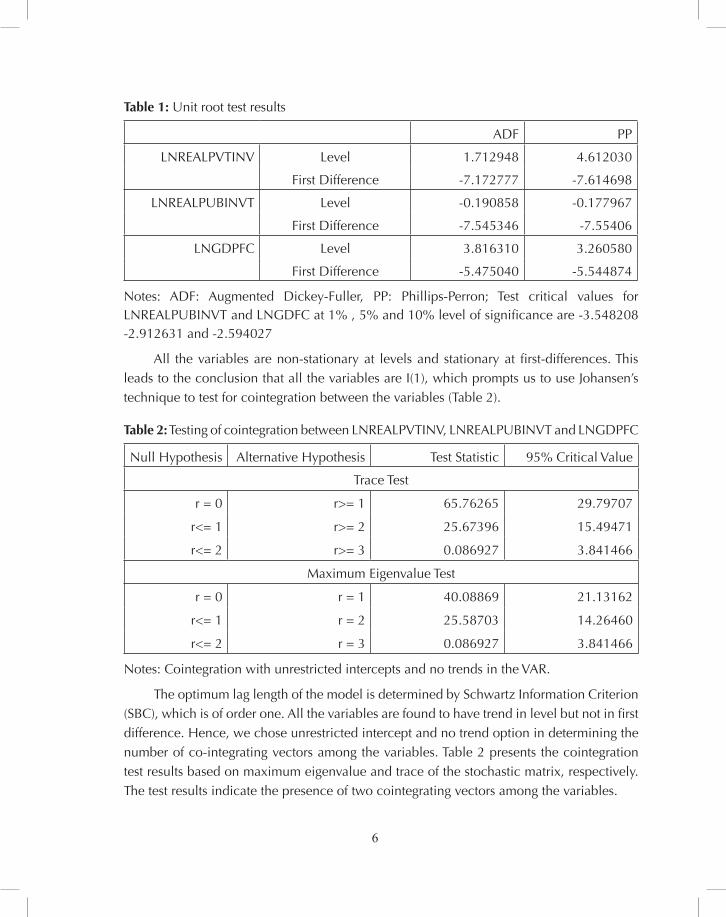
Table 1: Unit root test results

ADF PP

LNREALPVTINV Level 1.712948 4.612030

First Difference -7.172777 -7.614698

LNREALPUBINVT Level -0.190858 -0.177967

First Difference -7.545346 -7.55406

LNGDPFC Level 3.816310 3.260580

First Difference -5.475040 -5.544874

Notes: ADF: Augmented Dickey-Fuller, PP: Phillips-Perron; Test critical values for LNREALPUBINVT and LNGDFC at 1% , 5% and 10% level of significance are -3.548208 -2.912631 and -2.594027

All the variables are non-stationary at levels and stationary at first-differences. This leads to the conclusion that all the variables are I(1), which prompts us to use Johansen’s technique to test for cointegration between the variables (Table 2).

Table 2: Testing of cointegration between LNREALPVTINV, LNREALPUBINVT and LNGDPFC

Null Hypothesis Alternative Hypothesis Test Statistic 95% Critical Value

Trace Test

r = 0 r>= 1 65.76265 29.79707

r<= 1 r>= 2 25.67396 15.49471

r<= 2 r>= 3 0.086927 3.841466

Maximum Eigenvalue Test

r = 0 r = 1 40.08869 21.13162

r<= 1 r = 2 25.58703 14.26460

r<= 2 r = 3 0.086927 3.841466

Notes: Cointegration with unrestricted intercepts and no trends in the VAR.

The optimum lag length of the model is determined by Schwartz Information Criterion (SBC), which is of order one. All the variables are found to have trend in level but not in first difference. Hence, we chose unrestricted intercept and no trend option in determining the number of co-integrating vectors among the variables. Table 2 presents the cointegration test results based on maximum eigenvalue and trace of the stochastic matrix, respectively. The test results indicate the presence of two cointegrating vectors among the variables.

7

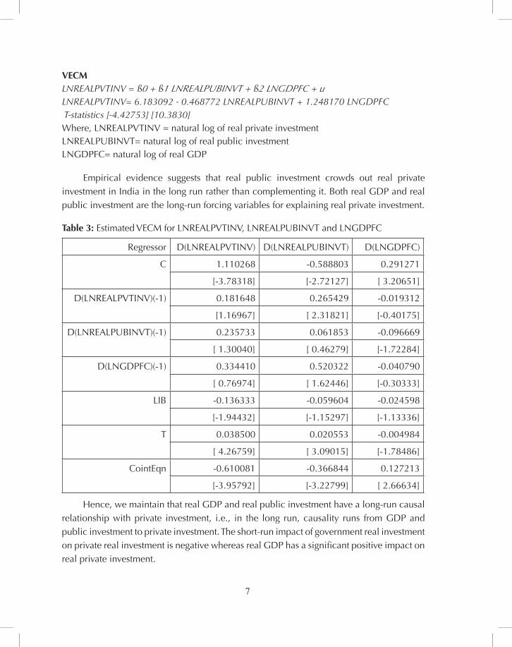
vECM LNREALPVTINV = ß0 + ß1 LNREALPUBINVT + ß2 LNGDPFC + uLNREALPVTINV= 6.183092 - 0.468772 LNREALPUBINVT + 1.248170 LNGDPFC T-statistics [-4.42753] [10.3830] Where, LNREALPVTINV = natural log of real private investment LNREALPUBINVT= natural log of real public investmentLNGDPFC= natural log of real GDP

Empirical evidence suggests that real public investment crowds out real private investment in India in the long run rather than complementing it. Both real GDP and real public investment are the long-run forcing variables for explaining real private investment.

Table 3: Estimated VECM for LNREALPVTINV, LNREALPUBINVT and LNGDPFC

Regressor D(LNREALPVTINV) D(LNREALPUBINVT) D(LNGDPFC)

C 1.110268 -0.588803 0.291271

[-3.78318] [-2.72127] [ 3.20651]

D(LNREALPVTINV)(-1) 0.181648 0.265429 -0.019312

[1.16967] [ 2.31821] [-0.40175]

D(LNREALPUBINVT)(-1) 0.235733 0.061853 -0.096669

[ 1.30040] [ 0.46279] [-1.72284]

D(LNGDPFC)(-1) 0.334410 0.520322 -0.040790

[ 0.76974] [ 1.62446] [-0.30333]

LIB -0.136333 -0.059604 -0.024598

[-1.94432] [-1.15297] [-1.13336]

T 0.038500 0.020553 -0.004984

[ 4.26759] [ 3.09015] [-1.78486]

CointEqn -0.610081 -0.366844 0.127213

[-3.95792] [-3.22799] [ 2.66634]

Hence, we maintain that real GDP and real public investment have a long-run causal relationship with private investment, i.e., in the long run, causality runs from GDP and public investment to private investment. The short-run impact of government real investment on private real investment is negative whereas real GDP has a significant positive impact on real private investment.

8

3. POLITICAL ECONOMy PERSPECTIvE Of fISCAL ADjUSTMENT

The main argument for the bias towards budget deficits and towards excess public spending has been given by the political economy approach. Alesina and Perotti (1995) classified three types of political economy models of fiscal policy: (1) models based on fiscal illusion with optimistic and naïve voters; (2) models of debt as a strategic variable; and (3) models of distributional conflict.

Models based on fiscal illusion with opportunistic and naïve votersPolicy makers are opportunistic. There is the electoral motive towards high spending in election years; the fiscal deficit increases in this way. Government spending increases before elections to improve reelection prospects. In developing countries, fiscal manipulation before elections is usually strong. Voters value public spending but consistently underestimate its costs in terms of the tax burden, especially if those costs are postponed. According to a classic argument, individuals favour expenditure but do not want to pay for it. Wagner (1976) and Buchanan and Wagner (1977) explained the notion of a ‘deficit illusion’ whereby voters do not understand the government’s inter-temporal budget. Voters usually overestimate expenditure value and underestimate expenditure cost if it is in terms of a future tax burden. Voters suffer from ‘fiscal illusion’ both in considering the size of government and in analysing budget deficits. Opportunistic incumbents take advantage of this misperception, running deficits to win the favour of voters. According to Ricardian equivalence, voters may not grasp fully the mechanics of the inter-temporal budget constraint by which today’s deficits are inevitably linked to tomorrow’s taxes and non-interest spending capacity. Voters do not punish politicians for fiscally irresponsible behaviour. Thus, voters support policy makers who provide high levels of deficit-financed expenditure and do not favour fiscally conservative politicians. This generates incentives for fiscal irresponsibility. It also generates asymmetric stabilisation policies, as policy makers are willing to run deficits to fight a recession but are not willing to run surpluses in good times. Voters measure the size of the government by their tax bill, and policy makers can disguise taxes so that voters underestimate the true tax bill.

Models of debt as a strategic variableThis model emphasises that the stock of debt affects policy choices of future governments and can therefore be used to constrain its action (Alesina and Tabellini 1990). In this context, a deficit bias can arise because different political parties, which face electoral uncertainties, have conflicting spending priorities. Governments at any time do not fully internalise the cost of running a budget deficit because the future spending that is going to be compressed may reflect the priorities of a different government. This deficit bias is increasing in the degree of political polarisation (reflected in the difference between spending priorities). In

9

this class of model, priorities before an election would agree on abandoned budget rule, but after the election, the party in power prefers discretion.

Models of distributional conflictA high level of fiscal deficit is the result of distributional conflicts between policy makers or between groups of voters. There is conflict between politicians with heterogeneous preferences who fear being replaced with different fiscal preferences and conflict between groups of voters with conflicting interests for a common pool of government revenues. Conflict between groups (represented by parties, interest groups, and coalition members) can delay the adoption of necessary policy measures, such as spending cuts or tax increases to stem growth in public indebtedness caused by exogenous factors (Alesina and Drazen 1991; Drazen and Grilli 1993). Delays occur because groups cannot agree on burden-sharing for the necessary fiscal adjustment. These models predict that fragmented or divided government and polarised societies will have more difficulty implementing fiscal adjustment than single-party governments and less polarised societies. Evidence presented in Roubini and Sachs (1989) and Grilli, Masciandaro, and Tabellini (1991) for OECD countries and in Poterba (1994) and Alt and Lowry (1994) for the US is consistent with these predictions. There is a common pool problem, where competition among different groups over the distribution of government revenues leads to deficits. Incumbent officials may also have incentives to run deficits to tie the hands of their successors. Current budget deficits impose costs in terms of either lower future public spending or higher future tax collections.

The model has three basic implications:officials from different parties, who are assumed to have heterogeneous preferences, (1) spend on different types of public goods; budget deficits increase with the probability that the government will be replaced; and(2) deficits increase with the level of polarisation between the different parties, since (3) greater polarisation implies larger differences between the preferences of the incum-bent and those of his potential replacement.

Heterogeneous interests across groups of voters have been put forward as a reason for potentially pervasive deficits. Weingast et al. (1981) argued that geographically diverse interests influence the budget. The problem arises if legislators making budget decisions represent geographic units interested in different government-funded projects but government revenues are centralised. The benefits of a given government project are then concentrated geographically, while its costs are shared by all districts. The consequence is that each district internalises the full benefit of specific projects but only part of the cost, which results in over-provision of government projects. The size of the budget, and thus the deficit, increases with the number of districts represented in the government; this phenomenon is termed government ‘fragmentation’.

10

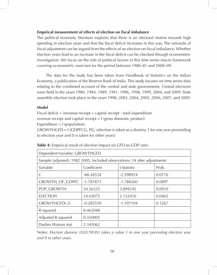
Empirical measurement of effects of election on fiscal imbalanceThe political economy literature explains that there is an electoral motive towards high spending in election years and that the fiscal deficit increases in this way. The rationale of fiscal adjustment can be argued from the effects of an election on fiscal imbalance. Whether election years lead to an increase in the fiscal deficit can be checked through econometric investigation. We focus on the role of political factors in this time series macro framework covering econometric exercises for the period between 1980–81 and 2008–09.

The data for the study has been taken from Handbook of Statistics on the Indian Economy, a publication of the Reserve Bank of India. This study focuses on time series data relating to the combined account of the central and state governments. Central elections were held in the years 1980, 1984, 1989, 1991, 1996, 1998, 1999, 2004, and 2009. State assembly election took place in the years 1998, 2003, 2004, 2005, 2006, 2007, and 2009.

ModelFiscal deficit = (revenue receipt + capital receipt - total expenditurerevenue receipt and capital receipt = f (gross domestic product)Expenditure = f (population) GROWTHGFD = f {GDPFCG, PG, (election is taken as a dummy 1 for one year proceeding to election year and 0 is taken for other years}

Table 4: Empirical result of election impact on GFD-to-GDP ratio

Dependent Variable: GROWTHGFD

Sample (adjusted): 1982 2005, Included observations: 24 after adjustments

Variable Coefficient t-Statistic Prob.

C -68.44534 -2.598924 0.0176

GROWTH_OF_GDPFC -1.781873 -1.788360 0.0897

POP_GROWTH 54.36325 3.894245 0.0010

ELECTION 14.65075 2.132416 0.0462

GROWTHGFD(-2) -0.285550 -1.597194 0.1267

R-squared 0.463048

Adjusted R-squared 0.350005

Durbin-Watson stat 2.345062

Notes: Election dummy (ELECTION) takes a value 1 in one year preceding election year and 0 in other years.

11

GDFCG = GDP growth rate at factor costPG = population growth rate Election = Election is taken as a dummy 1 for one year proceeding to election year and 0 is taken for other yearsGROWTHGFD = Growth of gross fiscal deficit (combined government)

From the empirical results given in Table 4, we can say that in India, elections significantly raise the fiscal deficit-to-GDP ratio whereas GDP growth (at factor price) lowers it.

5. EvOLUTION Of fISCAL ADjUSTMENT POLICy IN INDIA

India has been tackling fiscal deterioration by adopting a fiscal adjustment mechanism to improve fiscal stability. In the past decade, India has enacted mechanisms to bind governments to fiscal rectitude through formal legal or even constitutional devices. This section analyses certain major fiscal adjustment mechanisms.

In 2000–01, the Ministry of Finance issued guidelines to the states for Medium-Term Fiscal Reform Programmes (MTFRPs). It aimed at reducing wasteful expenditure (cutting low-priority spending) and improving tax collection or improving the efficiency of the tax administration. The MTFRPs required states to make time-bound reform in fiscal administration, power, public sector, and the budget and aimed at reducing the consolidated fiscal deficit to sustainable levels by 2005, as well as the debt-to-GDP ratio and interest payments. The MTFRPs could not achieve its target; rather, the fiscal situation deteriorated during this period. There was a design failure in prescribing a uniform 5-percentage-point improvement in the ratio for all states. If states started with larger base year deficits, it became relatively easier for them to make huge improvements.

In April 2000, the Eleventh Finance Commission (EFC)1 recommended an incentive fund in the form of the Fiscal Reform Facility (FRF) for fiscal adjustment. The EFC recommended the release of a 15 per cent grant to states by linking it with improvement in fiscal performance. Under the FRF, the Government of India prescribed that each state must achieve a minimum improvement of 5 per cent in revenue deficit/surplus as a proportion of its revenue receipts each year until 2004–05 measured with reference to the base year 1999–2000. As only a minor portion of the grants of non-plan revenue accounts was linked to fiscal performance, it did not incentivise states towards fiscal responsibility.

1 The Finance Commission is a constitutional body established under Article 280 of the Constitution of India every five years, primarily to determine the sharing of centrally collected tax proceeds between the central and state governments and the distribution of grants-in-aid of revenues across states. The terms of reference of the Finance Commission can be expanded by an Order of Parliament.

12

In the tax devolution process, considering the urgency of fiscal consolidation, various finance commissions of India have from time to time taken certain steps such as tax effort and fiscal discipline and have assigned them certain weights. Though the transfer formulae contain weights for efficiency (‘tax effort’2, fiscal discipline,3 etc.), their effects are often perceived to be weak and are subdued by equity factors.

The Twelfth Finance Commission (TWFC) recommended the debt write-off scheme to improve states’ fiscal prudence but also that each state enact a fiscal responsibility law and try to eliminate revenue deficit and reduce fiscal deficit. The debt write-off scheme became linked with the reduction of revenue deficit of the states. The quantum of repayment was linked to the absolute amount by which the revenue deficit was reduced in each successive year during the award period.

The Thirteenth Finance Commission has recommended that two debt relief measures be extended to all states. The first is that the interest rate on loans from the National Small Savings Fund (NSSF) to states contracted until 2006–07 and outstanding as of 2009–10 be reset at 9 per cent and structural reforms be brought in to link the NSSF to the market. The second debt relief recommended by the Commission is the write-off of Central loans to states. All the above-mentioned debt relief is available to states only if they amend/legislate fiscal responsibility and budget management (FRBM) Acts according to the Commission’s recommendations. The Commission has also recommended that states be eligible for Specific Grants only if they comply with this condition.

Even though initiatives have been taken to achieve fiscal responsibility, reform has been piecemeal. A widespread deterioration in the fiscal position with an associated impact on fiscal sustainability, macroeconomic vulnerability, and economic growth led to an emerging consensus on the urgent need for imposing statutory ceilings on the central government’s borrowings, debt, and deficits. Therefore, in 2003, the Government of India enacted the FRBM Act..

FRBM ActThe FRBM Act requires that the centre’s fiscal deficit be reduced to 3 per cent of GDP and that the revenue deficit be reduced by an amount equivalent to 0.5 per cent or more of GDP at the end of each year beginning with 2004–05 and eliminated by 2013–14. The fiscal deficit was to be reduced by 0.3 per cent or more of GDP at the end of each financial

2 The Tenth Finance Commission (TFC) took tax effort as a criterion for tax devolution to a state for the first time. It worked as an incentive among states to raise the tax potential capacity. The tax effort was measured by the ratio of per capita own tax revenue of a state to its per capita income. It was weighted by the inverse of per capita income.

3 The Eleventh Finance Commission introduced the fiscal discipline criterion for tax devolution for the first time. The index of fiscal discipline was arrived at by relating the improvement in the ratio of own revenue receipts of a state to its total revenue expenditure to average ratio across all the states.

13

year beginning with 2004–05. The debt-to-GDP ratio is required to be reduced by 68 per cent by 2014–15. In response to the debt relief package recommended by the Finance Commission in return for fiscal correction, almost every state except West Bengal and Sikkim has enacted fiscal responsibility acts. State governments accepted similar obligations of reducing fiscal deficit to 3 per cent of gross state domestic product (GSDP) and eliminating revenue deficits by 2013–14.

The FRBM Act takes suitable measures to ensure greater transparency in its fiscal operations. To ensure greater transparency in fiscal operations and the public interest, it requires the central government to disclose any significant change in accounting standards, policies, and practices affecting or likely to affect the computation of prescribed fiscal indicators when presenting annual financial statements and demands for grant. The government must present statements on medium-term fiscal policy, the macroeconomic framework, and the fiscal policy strategy statement each financial year. The medium-term fiscal policy statement of the central government must set a three-year rolling target as a percentage of GDP on four fiscal indicators: revenue deficit, fiscal deficit, tax revenue, and total outstanding liabilities. The fiscal policy strategy statement contains policies for the ensuing financial year on taxation, expenditure, market borrowing and other liabilities, lending and investment, pricing of administered goods and services, securities, and description of other activities such as underwriting and guarantees that have potential budgetary implications. The macroeconomic framework statement assesses the GDP, the fiscal balance of the union government (revenue balance and gross fiscal balance), and the external sector balance of the economy reflected in the current account balance of the BoP. The FRBM Act has an exclusion clause, under which the government may deviate from pre-specified fiscal targets if there are unforeseeable demands on government finances arising out of internal disturbances or natural calamity or such exceptional grounds as the government may specify.

However, doubts remain about how helpful the FRBM will be in attaining the primary objectives as distinguished from the intermediate ones of reducing deficit and debt. Some developmental economists argue that limiting fiscal deficit to 3 per cent may be too restrictive, although it may affect development expenditure or social expenditure (Ghosh and Sekhar 2005). They also argue that if the objective of an economy is employment generation, public expenditure through borrowing finance is useful. On the other hand, a society with egalitarian goals should aim to keep down fiscal deficit and finance public expenditure through progressive taxation (Patnaik 2006). The most important argument in favour of introducing a fiscal Policy Rule is the failure in the past 10 years to produce fiscal adjustment in India at the central or state level. India’s public deficit bias and indebtedness cannot be sustained much longer with stepped-up external liberalisation. Thus, there is a strong case for adopting transparent fiscal responsibility legislation with well-designed policy rules at national and sub-national levels of government (Kopits 2001).

14

Any rule-based fiscal adjustment programme may lead to fiscal stability on one hand but to distortions in the composition of government expenditure or tax increases on the other. This section analyses the major fiscal indicators to understand the suitability and effectiveness of the FRBM Act.

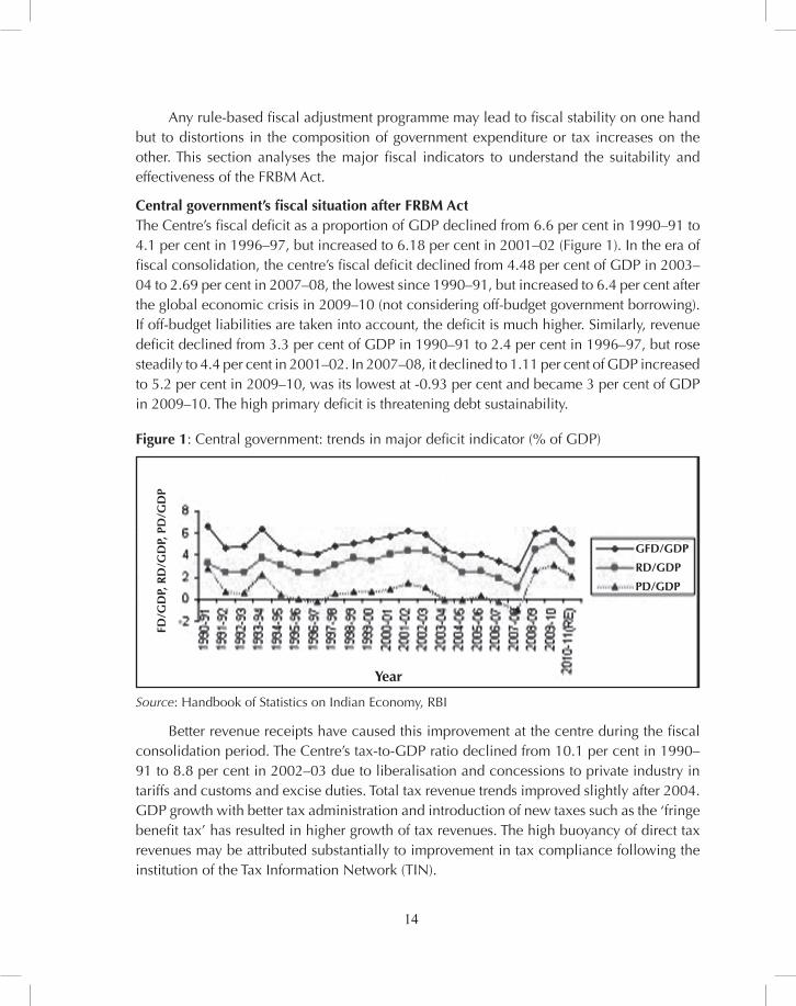
Central government’s fiscal situation after FRBM ActThe Centre’s fiscal deficit as a proportion of GDP declined from 6.6 per cent in 1990–91 to 4.1 per cent in 1996–97, but increased to 6.18 per cent in 2001–02 (Figure 1). In the era of fiscal consolidation, the centre’s fiscal deficit declined from 4.48 per cent of GDP in 2003–04 to 2.69 per cent in 2007–08, the lowest since 1990–91, but increased to 6.4 per cent after the global economic crisis in 2009–10 (not considering off-budget government borrowing). If off-budget liabilities are taken into account, the deficit is much higher. Similarly, revenue deficit declined from 3.3 per cent of GDP in 1990–91 to 2.4 per cent in 1996–97, but rose steadily to 4.4 per cent in 2001–02. In 2007–08, it declined to 1.11 per cent of GDP increased to 5.2 per cent in 2009–10, was its lowest at -0.93 per cent and became 3 per cent of GDP in 2009–10. The high primary deficit is threatening debt sustainability.

Figure 1: Central government: trends in major deficit indicator (% of GDP)

Source: Handbook of Statistics on Indian Economy, RBI

Better revenue receipts have caused this improvement at the centre during the fiscal consolidation period. The Centre’s tax-to-GDP ratio declined from 10.1 per cent in 1990–91 to 8.8 per cent in 2002–03 due to liberalisation and concessions to private industry in tariffs and customs and excise duties. Total tax revenue trends improved slightly after 2004. GDP growth with better tax administration and introduction of new taxes such as the ‘fringe benefit tax’ has resulted in higher growth of tax revenues. The high buoyancy of direct tax revenues may be attributed substantially to improvement in tax compliance following the institution of the Tax Information Network (TIN).

fD/G

DP,

RD

/GD

P, P

D/G

DP

GfD/GDP

RD/GDP

PD/GDP

year

15

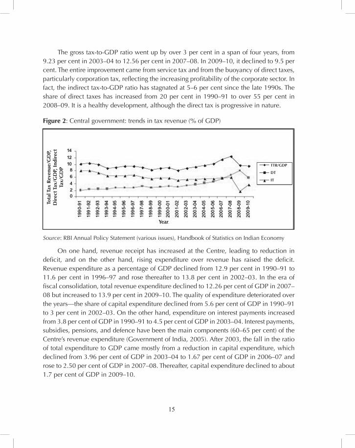
The gross tax-to-GDP ratio went up by over 3 per cent in a span of four years, from 9.23 per cent in 2003–04 to 12.56 per cent in 2007–08. In 2009–10, it declined to 9.5 per cent. The entire improvement came from service tax and from the buoyancy of direct taxes, particularly corporation tax, reflecting the increasing profitability of the corporate sector. In fact, the indirect tax-to-GDP ratio has stagnated at 5–6 per cent since the late 1990s. The share of direct taxes has increased from 20 per cent in 1990–91 to over 55 per cent in 2008–09. It is a healthy development, although the direct tax is progressive in nature.

Figure 2: Central government: trends in tax revenue (% of GDP)

Source: RBI Annual Policy Statement (various issues), Handbook of Statistics on Indian Economy

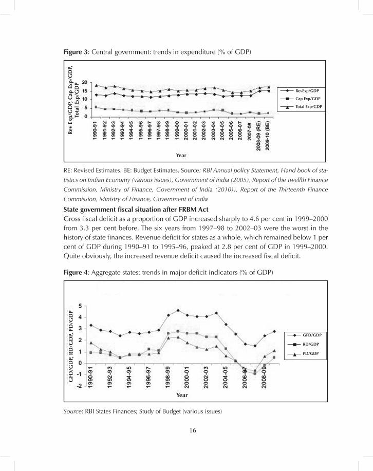
On one hand, revenue receipt has increased at the Centre, leading to reduction in deficit, and on the other hand, rising expenditure over revenue has raised the deficit. Revenue expenditure as a percentage of GDP declined from 12.9 per cent in 1990–91 to 11.6 per cent in 1996–97 and rose thereafter to 13.8 per cent in 2002–03. In the era of fiscal consolidation, total revenue expenditure declined to 12.26 per cent of GDP in 2007–08 but increased to 13.9 per cent in 2009–10. The quality of expenditure deteriorated over the years—the share of capital expenditure declined from 5.6 per cent of GDP in 1990–91 to 3 per cent in 2002–03. On the other hand, expenditure on interest payments increased from 3.8 per cent of GDP in 1990–91 to 4.5 per cent of GDP in 2003–04. Interest payments, subsidies, pensions, and defence have been the main components (60–65 per cent) of the Centre’s revenue expenditure (Government of India, 2005). After 2003, the fall in the ratio of total expenditure to GDP came mostly from a reduction in capital expenditure, which declined from 3.96 per cent of GDP in 2003–04 to 1.67 per cent of GDP in 2006–07 and rose to 2.50 per cent of GDP in 2007–08. Thereafter, capital expenditure declined to about 1.7 per cent of GDP in 2009–10.

Tota

l Tax

Rev

enue

/GD

P,

Dir

ect T

ax/G

DP,

Ind

irec

t Ta

x/G

DP

TTR/GDP

DT

IT

year

16

Figure 3: Central government: trends in expenditure (% of GDP)

RE: Revised Estimates. BE: Budget Estimates, Source: RBI Annual policy Statement, Hand book of sta-

tistics on Indian Economy (various issues), Government of India (2005), Report of the Twelfth Finance

Commission, Ministry of Finance, Government of India (2010)), Report of the Thirteenth Finance

Commission, Ministry of Finance, Government of India

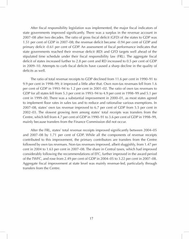
State government fiscal situation after FRBM ActGross fiscal deficit as a proportion of GDP increased sharply to 4.6 per cent in 1999–2000 from 3.3 per cent before. The six years from 1997–98 to 2002–03 were the worst in the history of state finances. Revenue deficit for states as a whole, which remained below 1 per cent of GDP during 1990–91 to 1995–96, peaked at 2.8 per cent of GDP in 1999–2000. Quite obviously, the increased revenue deficit caused the increased fiscal deficit.

Figure 4: Aggregate states: trends in major deficit indicators (% of GDP)

Source: RBI States Finances; Study of Budget (various issues)

Rev

Exp

/GD

P, C

ap E

xp/G

DP,

To

tal E

xp/G

DP

GfD

/GD

P, R

D/G

DP,

PD

/GD

P

RevExp/GDP

Cap Exp/GDP

Total Exp/GDP

GfD/GDP

RD/GDP

PD/GDP

year

year

17

After fiscal responsibility legislation was implemented, the major fiscal indicators of state governments improved significantly. There was a surplus in the revenue account in 2007–08 after two decades. The ratio of gross fiscal deficit (GFD) of the states to GDP was 1.51 per cent of GDP in 2007–08; the revenue deficit became -0.94 per cent of GDP and primary deficit -0.61 per cent of GDP. An assessment of fiscal performance indicates that state governments reached their revenue deficit (RD) and GFD targets well ahead of the stipulated time schedule under their fiscal responsibility law (FRL). The aggregate fiscal deficit of states increased further to 2.8 per cent and RD increased to 0.5 per cent of GDP in 2009–10. Attempts to curb fiscal deficits have caused a sharp decline in the quality of deficits as well.

The ratio of total revenue receipts to GDP declined from 11.6 per cent in 1990–91 to 9.9 per cent in 1998–99; it improved a little after that. Own non-tax revenues fell from 1.6 per cent of GDP in 1993–94 to 1.2 per cent in 2001–02. The ratio of own tax revenues to GDP for all states fell from 5.3 per cent in 1993–94 to 4.9 per cent in 1998–99 and 5.1 per cent in 1999–00. There was a substantial improvement in 2000–01, as most states agreed to implement floor rates in sales tax and to reduce and rationalise various exemptions. In 2007–08, states’ own tax revenue improved to 6.7 per cent of GDP from 5.5 per cent in 2002–03. The slowest growing item among states’ total receipts was transfers from the Centre, which fell from 4.7 per cent of GDP in 1990–91 to 3.6 per cent of GDP in 1998–99, mainly because transfers from the Finance Commission did not occur.

After the FRL, states’ total revenue receipts improved significantly between 2004–05 and 2007–08 by 1.71 per cent of GDP. While all the components of revenue receipts contributed to this improvement, the primary contributors are transfers from the Centre followed by own tax revenues. Non-tax revenues improved, albeit sluggishly, from 1.47 per cent in 2004 to 1.63 per cent in 2007–08. The share in Central taxes, which had improved considerably following the recommendations of EFC, further improved in the award period of the TWFC, and rose from 2.49 per cent of GDP in 2004–05 to 3.22 per cent in 2007–08. Aggregate fiscal improvement at state level was mainly revenue-led, particularly through transfers from the Centre.

18

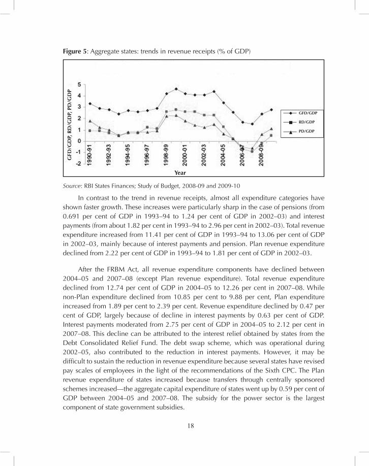
Figure 5: Aggregate states: trends in revenue receipts (% of GDP)

Source: RBI States Finances; Study of Budget, 2008-09 and 2009-10

In contrast to the trend in revenue receipts, almost all expenditure categories have shown faster growth. These increases were particularly sharp in the case of pensions (from 0.691 per cent of GDP in 1993–94 to 1.24 per cent of GDP in 2002–03) and interest payments (from about 1.82 per cent in 1993–94 to 2.96 per cent in 2002–03). Total revenue expenditure increased from 11.41 per cent of GDP in 1993–94 to 13.06 per cent of GDP in 2002–03, mainly because of interest payments and pension. Plan revenue expenditure declined from 2.22 per cent of GDP in 1993–94 to 1.81 per cent of GDP in 2002–03.

After the FRBM Act, all revenue expenditure components have declined between 2004–05 and 2007–08 (except Plan revenue expenditure). Total revenue expenditure declined from 12.74 per cent of GDP in 2004–05 to 12.26 per cent in 2007–08. While non-Plan expenditure declined from 10.85 per cent to 9.88 per cent, Plan expenditure increased from 1.89 per cent to 2.39 per cent. Revenue expenditure declined by 0.47 per cent of GDP, largely because of decline in interest payments by 0.63 per cent of GDP. Interest payments moderated from 2.75 per cent of GDP in 2004–05 to 2.12 per cent in 2007–08. This decline can be attributed to the interest relief obtained by states from the Debt Consolidated Relief Fund. The debt swap scheme, which was operational during 2002–05, also contributed to the reduction in interest payments. However, it may be difficult to sustain the reduction in revenue expenditure because several states have revised pay scales of employees in the light of the recommendations of the Sixth CPC. The Plan revenue expenditure of states increased because transfers through centrally sponsored schemes increased—the aggregate capital expenditure of states went up by 0.59 per cent of GDP between 2004–05 and 2007–08. The subsidy for the power sector is the largest component of state government subsidies.

GfD

/GD

P, R

D/G

DP,

PD

/GD

P

GfD/GDP

RD/GDP

PD/GDP

year

19

While the FRBM Act is a good attempt at fiscal consolidation both at the centre and in the states, its design has certain flaws.

It lacks clear accounting definitions to target fiscal indicators. This has allowed for creative accounting. For example, off-budget bonds have been issued to finance subsidies and have thus been excluded from the definition of the FRBMA-relevant deficit variable.

Budget preparation is opaque. Numerical targets have not been supported by comprehensive expenditure reform plans. Expenditures have consistently been underestimated in recent years, and particularly so if off-budget bonds are included. In addition, the assumptions underpinning the budget do not always include annual forecasts for key macroeconomic variables, and the discussion of fiscal risks is limited.

Historically, budget projections have been subject to systematic forecast errors. The FRBM Act focuses on a current balance target. This allows weaknesses in budget classification to be exploited, by misclassifying current expenditures as capital expenditures. Targeting the current balance may also bias spending against education and health, which have a large current expenditure component.

In addition, the international experience illustrates that deficit-type targets, such as the current balance, are more likely to reduce incentives for fiscal savings in good times, and to force adjustment in bad times (i.e. procyclicality).

There are no explicit automatic penalties for missing fiscal targets and/or not following budget procedures under the FRBM Act or the provision for an independent assessment of compliance with the FRBM Act.

6. CONCLUSION

Although reforms have been attempted occasionally to improve fiscal responsibility, they have been piecemeal. The fiscal situation deteriorated mainly because revenue expenditure exceeded revenue receipt. The expenditure on interest payments, subsidies, and pension accounts for a major portion of the total revenue expenditure. After the FRBM Act was implemented, circumstances at the Centre improved slightly because revenue (tax) receipts increased and expenditure was cut. While capital expenditure has declined drastically, revenue expenditure (such as interest and pension payments) has not changed much.

Fiscal adjustment programmes should also focus on capital expenditure, a major growth indicator, which should be increased. Target variables should be chosen so that adjustment does not affect the social sector or capital spending. The enactment of an FRL

20

in 26 states has resulted in significant fiscal correction. In aggregate, these states have reached their expenditure and debt targets ahead of schedule. Revenue buoyancy, both due to improved own tax revenues of the states and due to the derived benefit of high central tax buoyancies (through share in central taxes), has mainly been responsible for the fiscal correction. The aggregate finances of states improved significantly following higher growth of own tax revenues and increased transfers from the Centre. The revenue account of states turned surplus in 2006–07 and continued through 2007–08. This is ahead of the target date of 2008–09 recommended by the TWFC.

After the global financial crisis, fiscal sustainability became a question again. Major fiscal indicators like fiscal deficit and RD have become very high. Now, the role of a fiscal initiative is to control the fiscal imbalance, so that FRBM should be designed properly. There is a need to go beyond the budget in setting Fiscal Policy Rule targets, in particular to incorporate off-budget borrowing by state-level public sector undertakings and the power sector deficit. Contingent liabilities should be capped should be consolidated with on-budget borrowing along with off-budget borrowing if debt serving falls to government.

The most challenging reform task involves the re-examination of fiscal relations between the Centre and state governments to restore vertical balance and bring about fiscal responsibility. It is necessary to adopt a mechanism of intergovernmental relations with strong incentives at the sub-national level for expenditure control and revenue-raising. The recent agreement on indirect taxation at the state level is a key element in this regard. If such a mechanism is not developed, sub-national governments will continue to incur sizable deficits and rely on costly bailouts. Other structural reforms that should help adhere to fiscal rules include downsizing the government’s work force, further rationalisation of subsidies, and elimination or streamlining of quasi-fiscal operations.

21

References

Drazen, Allan. (2004). Fiscal Rules from a Political Economy Perspective. In George F. Kopits (ed.), Rules-Based Fiscal Policy in Emerging Markets: Background, Analysis, and Prospects (London: Palgrave Macmillan Economic Survey (2006-07), New Delhi.

Government of India. (2000a). Report of the (EAS Sarma) Committee on Fiscal Responsibility Legislation, Department of Economic Affairs, Ministry of Finance, Government of India.

Government of India. (2000b). The Fiscal Responsibility and Budget Management Bill, Bill No. 220 introduced in Lok Sabha: 29 December 2000, Ministry of Finance, Government of India.

Govt. of India. (2000). Report of the Eleventh Finance Commission, 2000–2005, Ministry of Finance, June, New Delhi.

Govt. of India. (2005). Report of the Twelfth Finance Commission, Ministry of Finance, 2005–10, New Delhi.

Govt. of India. (2010). Report of The Twelfth Finance Commission, Ministry of Finance, 2010–2015, New Delhi.

Howes, Stephen and Jha, Shikha. (2004). ‘State Finances in India: Towards Fiscal Responsibility’, in Edgardo M. Favaro and Ashok K. Lahiri (ed.), Fiscal Policies and Sustainable Growth in India Oxford University Press, New Delhi, 2004.

Indira, Rajaraman. (2006), ‘Fiscal Developments and Outlook in India’. In Peter S. Heller and M. Govinda Rao (ed.), A Sustainable Fiscal Policy for India—An International Perspective, Oxford University Press, New Delhi, 2006.

International Monetary Fund. (1995). ‘Guidelines for Fiscal Adjustment’, Pamphlet Series No. 49.

International Monetary Fund, (2006). ‘Fiscal Adjustment for Stability and Growth’, James Daniel (et al.), Washington D.C, Pamphlet series No. 55.

Kalpana, Kochhar. (2006). ‘India Macroeconomic Implications of the Fiscal Imbalances’. in Peter S. Heller and M. Govinda Rao (eds), A Sustainable Fiscal Policy For India—An International Perspective. Oxford University Press, New Delhi, 2006.

Kopits, George F. and Steven A. Symansky. (1998). ‘Fiscal Policy Rules’, IMF Occasional Paper No. 162 (Washington: International Monetary Fund).

Kopits, George F. (2001a). ‘Fiscal Rules: Useful Policy Framework or Unnecessary Ornament?’, IMF Working Paper 01/145 (Washington: International Monetary Fund).

Kopits, George. (2001b). ‘Fiscal Policy Rules of India’, Economic and Political Weekly, vol 36, March, pp 749-56

22

Ministry of Finance. (2004). ‘Report of the Task Force on Implementation of the Fiscal Responsibility and Budget Management Act, 2003’, New Delhi: Government of India.

Mukesh Anand, Bagchi, Amaresh and Sen, Tapas K. (2004). ‘Fiscal Incentives at the States Level: Perverse Incentives and Paths to Reform’, in Edgardo Favaro and Ashok Lahiri (ed.), Fiscal Policies and Sustainable Growth in India, Oxford University Press, New Delhi.

Patnaik, Prabhat. (2006). ‘What is Wrong with Sound Finance’, Economic and Political Weekly, Vol XLI Nos. 43 and 44, November 4–10, pp. 4553–9.

Rangarajan, C. and Srivastava, D.K. (2005). ‘Fiscal Deficits and Government Debt in India: Implications for Growth and Stabilization’, NIPFP Working Paper No. 35.

Rangarajan, C. and Subarao Duvvuri. (2007). ‘The Importance of Being Earnest About Fiscal Responsibility’, Monograph, Madras School of Economics.

Reserve Bank of India. (2005). Report of the Group on Model Fiscal Responsibility Legislation at States Level’

Rao, M. Govind, Sen, Tapas and Jena Pratap. (2008). ‘Issues before the Thirteenth Finance Commission’, NIPFP Working Paper, August 2008, pp. 2008-55,.

Ricardo Hausmann and Catriona Purfield. (2006). ‘The Challenges of Fiscal Adjustment in a Democracy: The Case of India’, in Peter S. Heller and M. Govinda Rao (eds), A Sustainable Fiscal Policy For India - An International Perspective, Oxford University Press, New Delhi.

Srivastava, D.K. (2008). ‘Fiscal Responsibility Rules in India: Impact and Reassessment’, V.K.R.V. Rao Centenary Conference on National Income and other Macroeconomic Aggregates in a Growing Economy, 28–30 April 2008, organised by Delhi School of Economics and Institute of Economic Growth.