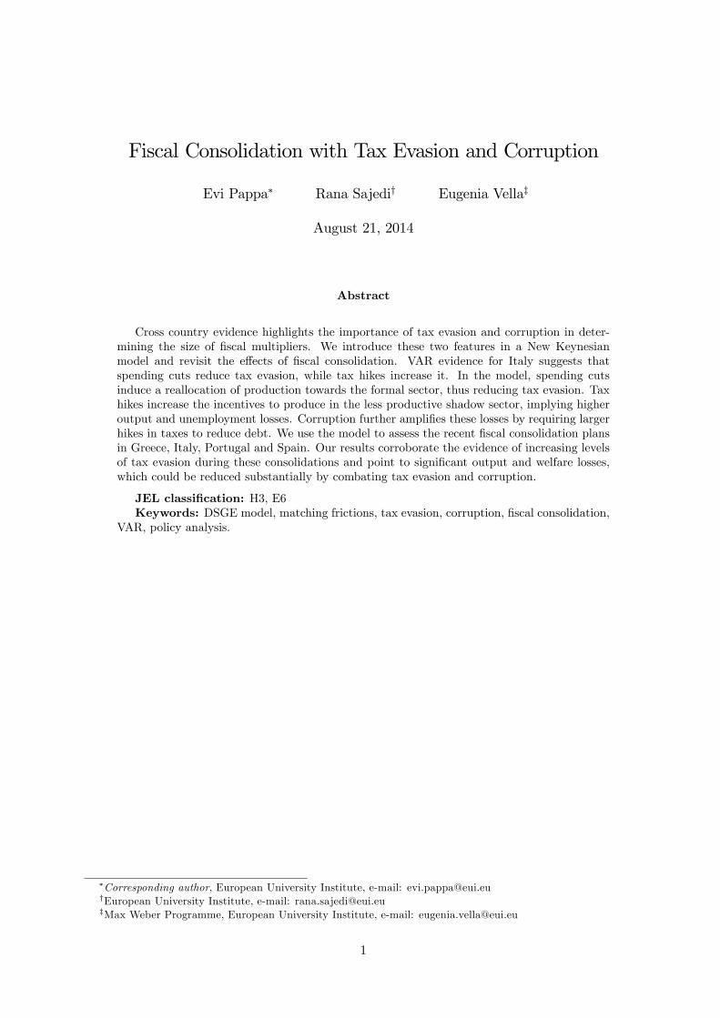
Fiscal Consolidation with Tax Evasion and Corruption

Evi Pappa� Rana Sajediy Eugenia Vellaz

August 21, 2014

Abstract

Cross country evidence highlights the importance of tax evasion and corruption in deter-mining the size of �scal multipliers. We introduce these two features in a New Keynesianmodel and revisit the e¤ects of �scal consolidation. VAR evidence for Italy suggests thatspending cuts reduce tax evasion, while tax hikes increase it. In the model, spending cutsinduce a reallocation of production towards the formal sector, thus reducing tax evasion. Taxhikes increase the incentives to produce in the less productive shadow sector, implying higheroutput and unemployment losses. Corruption further ampli�es these losses by requiring largerhikes in taxes to reduce debt. We use the model to assess the recent �scal consolidation plansin Greece, Italy, Portugal and Spain. Our results corroborate the evidence of increasing levelsof tax evasion during these consolidations and point to signi�cant output and welfare losses,which could be reduced substantially by combating tax evasion and corruption.

JEL classi�cation: H3, E6Keywords: DSGE model, matching frictions, tax evasion, corruption, �scal consolidation,

VAR, policy analysis.

�Corresponding author, European University Institute, e-mail: evi.pappa@eui.euyEuropean University Institute, e-mail: rana.sajedi@eui.euzMax Weber Programme, European University Institute, e-mail: eugenia.vella@eui.eu

1

1 Introduction

When there is an income tax, the just man will pay more and the unjust less on the same amount

of income. Plato, The Republic, Book I, 343-D

The recent �scal crisis has sparked a considerable amount of research measuring the macroeco-

nomic e¤ects of �scal consolidations.1 This literature, however, has left aside two crucial political

economy aspects, namely the presence of tax evasion and corruption. This is surprising, given that

they are important features in many of the countries adopting consolidation policies, as Figure 1

shows. In addition, there is growing evidence that tax evasion and corruption have increased in

recent years. For example, a recent report by the technical sta¤ of the Spanish Finance Ministry

(Gestha, 2014) indicates that the shadow economy increased by 6.8 percentage points between

2008 and 2012, reaching 24.6% of GDP. At the same time, a special Greek police task force re-

ported in 2013 that the number of cases of public corruption increased by 33% between 2011 and

2012.2 The aim of this paper is to revisit the e¤ects of government expenditure cuts and labor

tax hikes on output, unemployment and welfare, when tax evasion and corruption are present.

We treat tax evasion as synonymous with the shadow economy, which, according to Buehn and

Schneider (2012, p.175-176), comprises �all market-based, lawful production or trade of goods and

services deliberately concealed from public authorities in order to evade either payment of income,

value added or other taxes, or social security contributions�. Fiscal policy has an impact on the

size of the shadow economy since it a¤ects the incentives to tax evade both directly, through the

tax burden, and indirectly, through its e¤ects on the formal economy. Thus, a �scal consolidation

can have important secondary e¤ects if it generates a reallocation of resources between the formal

and informal sectors. Corruption, in this paper, refers to the embezzlement of public funds. The

presence of corruption can hamper the ability of the government to raise revenue, and thus distort

the e¤ects of �scal consolidations. Tax evasion and corruption often coexist and possibly interact.

For instance, Buehn and Schneider (2012) indicate that there is a positive correlation between the

two.

Many authors have studied whether it is preferable to rely on spending cuts or tax hikes when

consolidating de�cit. Overall, the �ndings are not conclusive. Using multi-year �scal consolidation

data for 17 OECD countries over the period 1980-2005, Alesina et al. (2013) show that expenditure-

based adjustments are typically associated with mild and short-lived recessions, and in some cases

with no recession at all, while tax-based corrections are followed by deep and prolonged recessions.

On the other hand, Erceg and Lindé (2013) reach a di¤erent conclusion. Using a two-country

Dynamic Stochastic General Equilibrium (DSGE) model of a currency union, they show that,

in the short run, a spending cut depresses output by more than a labor tax hike, because of the

limited accommodation by the central bank and the �xed exchange rate. However, this is reversed

in the long run as real interest and exchange rates adjust towards their �exible price levels.

1The implementation of the Maastricht Treaty in the mid 1990s initiated a wave of research on the e¤ects ofconsolidations. For examples, see the survey in Perotti (1996).

2See http://greece.greekreporter.com/2013/04/02/greek-police-public-worker-corruption-soars/

2

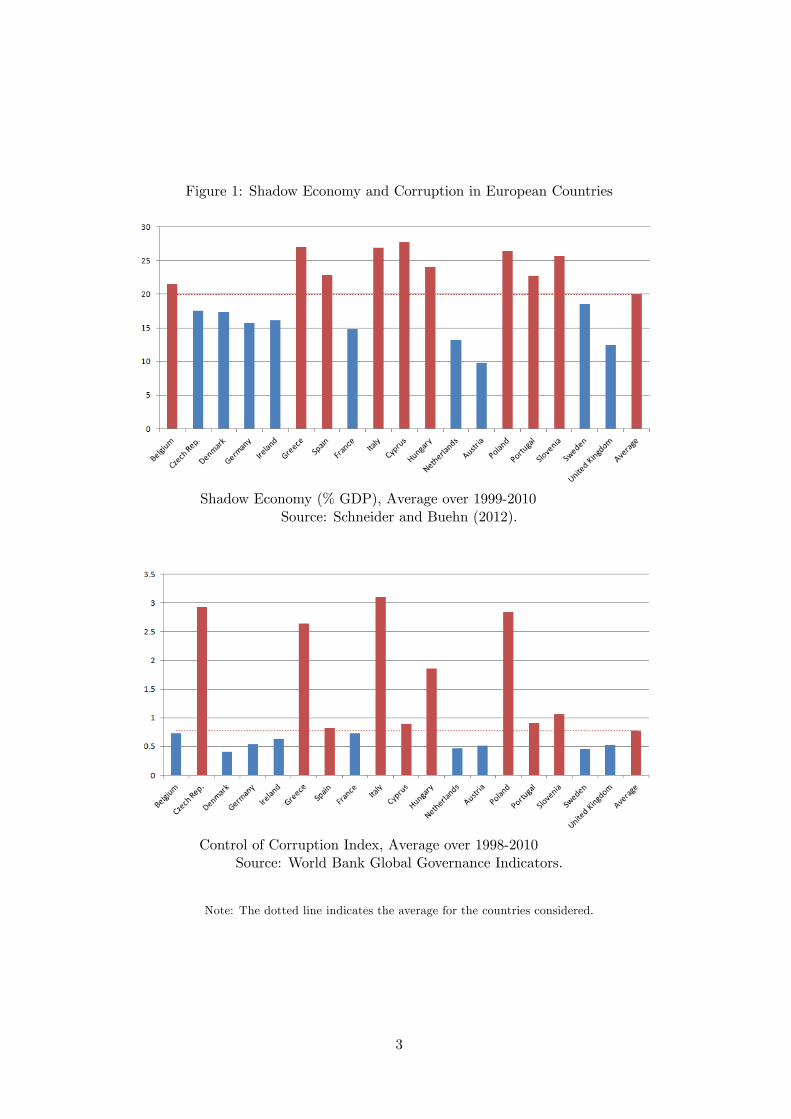
Figure 1: Shadow Economy and Corruption in European Countries

Shadow Economy (% GDP), Average over 1999-2010Source: Schneider and Buehn (2012).

Control of Corruption Index, Average over 1998-2010Source: World Bank Global Governance Indicators.

Note: The dotted line indicates the average for the countries considered.

3

Indeed, there is strong evidence that the e¤ects of �scal consolidations are not yet fully un-

derstood. Blanchard and Leigh (2013) examine the impact of the recent �scal consolidations in

26 OECD countries. They regress the forecast errors of output growth between 2010-2011 on the

planned consolidation of public de�cit, and �nd that the forecasts underestimate the size of �scal

multipliers. As shown in the next section, the underestimation of �scal multipliers is more pro-

nounced in countries with a higher level of tax evasion and/or corruption, suggesting that these

two features amplify the e¤ects of �scal consolidations.

Reliable time series data on tax evasion is typically hard to get. Luckily, the Italian National

Institute of Statistics (ISTAT) has created and regularly updated a time series of informal em-

ployment in Italy, which is consistent with international standards and, in particular, with the

1993 System of National Accounts. Apart from data availability, Italy is a �tting case for study-

ing tax evasion and corruption. Firstly, there is abundant evidence of a large shadow economy,

with estimates varying between 15% and 30% of GDP (see e.g. Ardizzi et al., 2012, Orsi et al.,

2014, and Schneider and Buehn, 2012). Secondly, Busato and Chiarini (2004) have shown that

incorporating the shadow economy in an RBC model for Italy considerably improves the �t to the

data. Thirdly, Italy scores poorly in international rankings of institutional quality: it is currently

ranked 72nd among 176 countries with a score of 42/100 in Transparency International�s Corrup-

tion Perception Index (henceforth COPI) and 25th among the 27 EU members in the index for

the �Quality of Government�(see Charron et al., 2012).3

In the �rst part of the paper, we incorporate the ISTAT series on informal employment in

a VAR, and identify the e¤ects of �scal consolidations occurring through a fall in government

consumption expenditure or an increase in direct taxes. We �nd that both types of shocks are

contractionary, both reducing output and increasing unemployment. However, tax hikes signi�-

cantly increase informal employment, while spending cuts reduce it.

To understand the mechanisms driving the results, we reassess the e¤ects of �scal consoli-

dations in a model with price stickiness, search and matching frictions, endogenous labor force

participation, tax evasion and corruption. The economy features a regular and an informal sector,

and the transactions in the latter sector are not recorded by the government. Firms can hire in-

formal labor to hide part of their production and evade payroll taxes. Households may also evade

personal income taxation by reallocating their labor to the informal sector. In each period, there

is a positive probability that irregular employment is detected, in which case the worker loses

the job and the �rm pays a �ne. Corruption implies that a fraction of tax revenues is embezzled.

Following Erceg and Lindé (2013), either labor tax rates or government consumption expenditures

react to the deviation of the debt-to-GDP ratio from a target value. Fiscal consolidation occurs

when this target is hit by a negative shock.

We �nd that the presence of tax evasion and corruption ampli�es the negative e¤ects of labor

tax hikes on output and unemployment, while it mitigates those of expenditure cuts. Tax evasion

and corruption imply that a larger increase in the tax rate is needed to reduce debt, and this

3The Corruption Perception Index is based on a cross country survey assessing the degree of transparency inpublic administration. The latter index accounts for other pillars, such as protection of the rule of law, governmente¤ectiveness and accountability, in addition to corruption.

4

ampli�es the distortionary e¤ects of the consolidation. Tax evasion further increases the output

losses after a tax hike because workers and �rms reallocate resources to the informal sector,

increasing ine¢ ciencies since this sector is less productive.

On the other hand, government spending cuts reduce tax evasion. The spending cut creates

a positive wealth e¤ect which increases consumption and investment and reduces labor force

participation. This wealth e¤ect leads to an investment boom, and a subsequent rise in the

capital stock, and agents reallocate their labor search towards the formal sector �rst because it

is more productive and second because the formal labor market has a higher matching e¢ ciency

and a lower job destruction rate. Hence, the share of shadow employment in total employment is

reduced. Relative to standard models, tax evasion and corruption increase the size of this wealth

e¤ect, thereby increasing the crowding-in of private consumption, and reducing output losses.

Labor tax hikes are costly in terms of welfare, but spending cuts typically involve welfare gains,

since private consumption increases and labor supply decreases. The latter result is reversed,

however, if government spending directly enters the utility of households, or if agents are liquidity

constrained.

We use our model to compare the recent consolidation policies in Greece, Italy, Spain and

Portugal, all countries that are characterized by both high corruption and tax evasion. Despite

the fact that the consolidation plans rely heavily on spending cuts, the model predicts increasing

levels of tax evasion in all countries, as well as prolonged recessions. Greece features the largest

output losses, due to the severity of the austerity measures. There are also substantial welfare

losses in all countries; the largest occurs in Portugal because of the signi�cant tax hikes in the

consolidation package.

There have been considerable discussions in the policy arena about combating both tax evasion

and corruption. For example, members of the European Parliament organized an event focusing

on corruption and tax evasion in Ljubljana in May 2013. The issue of reducing tax evasion also

dominated the 2013 meeting of G8 leaders. To quantitatively evaluate the welfare gains from

�ghting tax evasion and corruption, we perform a counterfactual analysis of the consolidation

plans when we reduce the degree of corruption and tax evasion. We �nd that both battles are

worth �ghting as they signi�cantly reduce the welfare losses from �scal consolidation.

The remainder of the paper is organized as follows. In the next section we present empirical

evidence to motivate our work. In Section 3 we develop the model and discuss the main theoretical

results. Section 4 presents the policy comparisons and Section 5 concludes.

2 Empirical Evidence

This section is divided in two parts. We �rst present evidence highlighting the importance of

corruption and tax evasion in determining the size of �scal multipliers. Here, we extend the

cross country regressions of Blanchard and Leigh (2013), henceforth BL (2013), controlling for

tax evasion and public corruption, and we check the robustness of our conclusions by considering

the output e¤ects of narrative consolidation shocks. We then use the ISTAT data on shadow

employment to run VAR regressions examining the e¤ects of spending cuts and tax hikes on

5

output, unemployment and shadow employment in Italy.

2.1 Do Tax Evasion and Corruption Matter?

To motivate our study, we replicate the BL (2013) regressions, controlling for tax evasion and

public corruption. As a proxy for tax evasion we use the estimates of the share of shadow output

to total GDP provided by Elgin and Öztunal¬(2012), while for corruption we use the COPI. We

group the 26 European countries considered by BL (2013) into either high and low tax evasion, or

high and low corruption.4 We then add to the BL (2013) regressions a dummy which is equal to

one for the high corruption or tax evasion group. We also run the same regression using a dummy

for both high corruption and tax evasion; in this case we drop three countries which do not fall

into the same group across the two indices.5

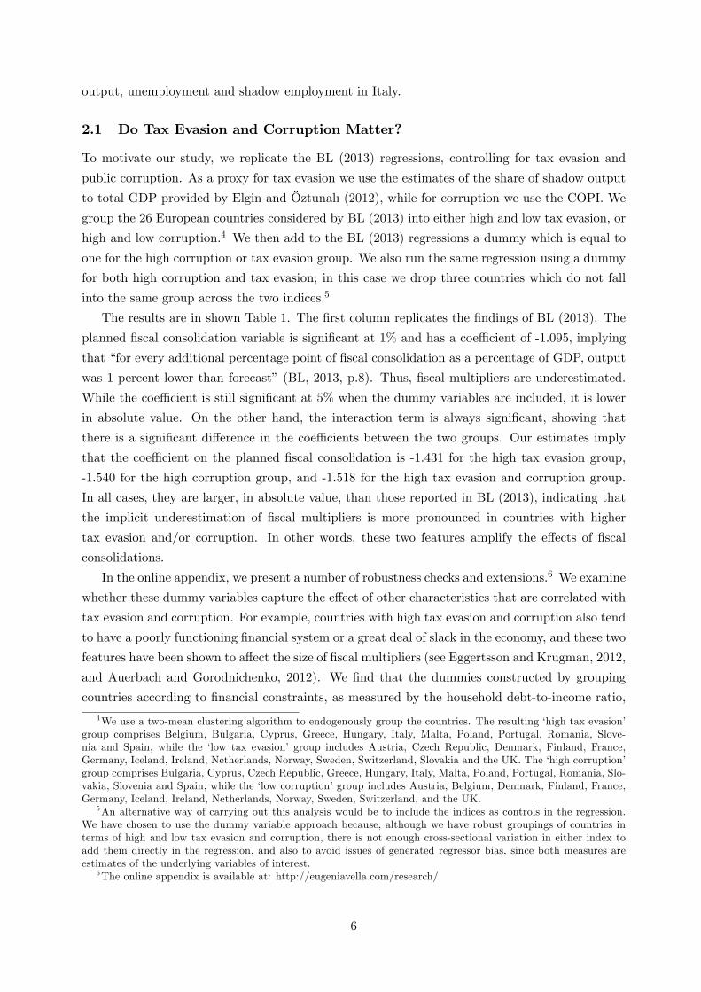
The results are in shown Table 1. The �rst column replicates the �ndings of BL (2013). The

planned �scal consolidation variable is signi�cant at 1% and has a coe¢ cient of -1.095, implying

that �for every additional percentage point of �scal consolidation as a percentage of GDP, output

was 1 percent lower than forecast�(BL, 2013, p.8). Thus, �scal multipliers are underestimated.

While the coe¢ cient is still signi�cant at 5% when the dummy variables are included, it is lower

in absolute value. On the other hand, the interaction term is always signi�cant, showing that

there is a signi�cant di¤erence in the coe¢ cients between the two groups. Our estimates imply

that the coe¢ cient on the planned �scal consolidation is -1.431 for the high tax evasion group,

-1.540 for the high corruption group, and -1.518 for the high tax evasion and corruption group.

In all cases, they are larger, in absolute value, than those reported in BL (2013), indicating that

the implicit underestimation of �scal multipliers is more pronounced in countries with higher

tax evasion and/or corruption. In other words, these two features amplify the e¤ects of �scal

consolidations.

In the online appendix, we present a number of robustness checks and extensions.6 We examine

whether these dummy variables capture the e¤ect of other characteristics that are correlated with

tax evasion and corruption. For example, countries with high tax evasion and corruption also tend

to have a poorly functioning �nancial system or a great deal of slack in the economy, and these two

features have been shown to a¤ect the size of �scal multipliers (see Eggertsson and Krugman, 2012,

and Auerbach and Gorodnichenko, 2012). We �nd that the dummies constructed by grouping

countries according to �nancial constraints, as measured by the household debt-to-income ratio,

4We use a two-mean clustering algorithm to endogenously group the countries. The resulting �high tax evasion�group comprises Belgium, Bulgaria, Cyprus, Greece, Hungary, Italy, Malta, Poland, Portugal, Romania, Slove-nia and Spain, while the �low tax evasion� group includes Austria, Czech Republic, Denmark, Finland, France,Germany, Iceland, Ireland, Netherlands, Norway, Sweden, Switzerland, Slovakia and the UK. The �high corruption�group comprises Bulgaria, Cyprus, Czech Republic, Greece, Hungary, Italy, Malta, Poland, Portugal, Romania, Slo-vakia, Slovenia and Spain, while the �low corruption�group includes Austria, Belgium, Denmark, Finland, France,Germany, Iceland, Ireland, Netherlands, Norway, Sweden, Switzerland, and the UK.

5An alternative way of carrying out this analysis would be to include the indices as controls in the regression.We have chosen to use the dummy variable approach because, although we have robust groupings of countries interms of high and low tax evasion and corruption, there is not enough cross-sectional variation in either index toadd them directly in the regression, and also to avoid issues of generated regressor bias, since both measures areestimates of the underlying variables of interest.

6The online appendix is available at: http://eugeniavella.com/research/

6

Table 1: Blanchard and Leigh (2013) Regressions with Additional ControlsDependent Variable: Forecast Error of GDP growth

1 2 3 4

REGRESSORS (Baseline)

Planned Fiscal Consolidation -1.095*** -0.670** -0.550** -0.618**

(0.255) (0.268) (0.259) (0.268)

Interaction with:

High Tax Evasion -0.761**

(0.351)

High Corruption -0.990***

(0.333)

High Tax Evasion -0.900**

and Corruption (0.351)

Constant 0.775* 0.918** 0.964** 0.925*

(0.383) (0.414) (0.415) (0.450)

Observations 26 26 26 23

R-squared 0.496 0.557 0.600 0.607

Robust standard errors in parentheses���p � 0:01; ��p � 0:05; �p � 0:1

or the level of slack in the economy, as measured by the unemployment rate, are not signi�cant.

We also run regressions for the components of GDP, and for unemployment, to understand which

variables are more signi�cantly a¤ected by the presence of these two features. We �nd that the

presence of corruption and tax evasion is particularly important for the e¤ects of consolidations

on the unemployment rate and investment, but not for consumption, exports or imports.

The BL (2013) methodology has been criticized in a number of ways. Of particular importance

for our study is the fact that the regression may not truly capture the e¤ect of �scal multipliers

on forecast errors. Given that the forecasts are conditional not only on �scal shocks but on the

full set of information used by the forecaster, forecast errors may depend on factors other than

underestimated �scal multipliers.

In order to check whether the results we obtain are due to the particular methodology of BL

(2013), we perform a di¤erent exercise using the narrative �scal consolidation episodes identi�ed

by Devries et al. (2011) for a group of OECD countries. As above, we separate the sample of

countries into high and low tax evasion and high and low corruption groups.7 We then calculate

7 In this case, the �high tax evasion�group consists of Belgium, Ireland, Italy, Portugal and Spain, whilst the �lowtax evasion�group consists of Australia, Austria, France, the UK and the US. The �high corruption�group consists

7

the output responses to both expenditure-based and tax-based consolidations for each group by

estimating an empirical model similar to Alesina et al. (2013). The results are shown in Figure

2. Tax evasion and corruption do not appear to signi�cantly a¤ect the response of output to

expenditure-based consolidations, although the high tax evasion group has slightly lower output

losses in the long run. In the case of tax-based consolidations, the output e¤ects for high tax

evasion and corruption countries are lower on impact, but signi�cantly larger and more prolonged

in the medium and long run. Hence, even with this alternative methodology, we �nd that tax

evasion and corruption a¤ect the size of �scal multipliers, and amplify the output losses from tax

adjustments in particular.8

2.2 Do Fiscal Consolidations A¤ect Tax Evasion?

The Italian statistical o¢ ce provides estimates of the number of employees working in the informal

sector using the discrepancies between reported employment from household surveys and �rm

surveys (see ISTAT, 2010). We use the share of informal workers in total workers as a measure

of the size of the shadow economy, and enter this variable into a VAR to ascertain the e¤ect of

�scal consolidations using di¤erent instruments.

To identify the e¤ects of unexpected spending cuts, we run a VAR with GDP (or the un-

employment rate), government �nal consumption expenditures, government debt and the share

of informal workers in total workers as endogenous variables, and tax revenues as an exogenous

variable. We use sign restrictions to identify a negative shock to government expenditure which

lasts for 3 periods, and reduces debt with a lag. To identify the e¤ects of unexpected labor tax

hikes, we run a similar VAR which includes direct tax revenues as an endogenous variable and

government expenditures as an exogenous control. We again use sign restrictions to identify a

positive shock to tax revenues, lasting 3 periods, which reduces debt with a lag. The responses of

all other variables are left unrestricted. The sign restrictions used are summarized in Table 2.

We use annual data from 1980-2006. Except for the ISTAT series, all data is taken from the

AMECO database of the European Commission.9 All �scal variables are expressed as a ratio to

GDP, and we include time trends and dummies for the start of the European Monetary Union,

and for the mid-90s since there is a break in the debt series. We include one lag in the VAR, and

also include interest rates as an exogenous variable in order to control for the e¤ects of monetary

policy. Given the small sample size, we estimate the VAR with Bayesian methods and present

68% posterior con�dence bands.

Figures 3 and 4 show the resulting IRFs.10 After an expenditure cut, output decreases sig-

ni�cantly at all horizons, while shadow employment falls signi�cantly on impact. Following a tax

hike, output does not fall on impact but the response is signi�cantly negative in the medium run,

of France, Italy, Japan, Portugal and Spain, and the �low corruption�group consists of Australia, Austria, Denmark,Finland and Sweden.

8As above, we have examined whether these di¤erences arise due to di¤erences in the �nancial system, or thedegree of slack in the economy, and do not �nd evidence in the data supporting this hypothesis.

9The ISTAT data is available from http://www.istat.it/it/archivio/39522.10For ease of exposition we show only the responses of the unrestricted variables in each case; the other responses

are in line with the sign restrictions imposed and are presented in the online appendix.

8

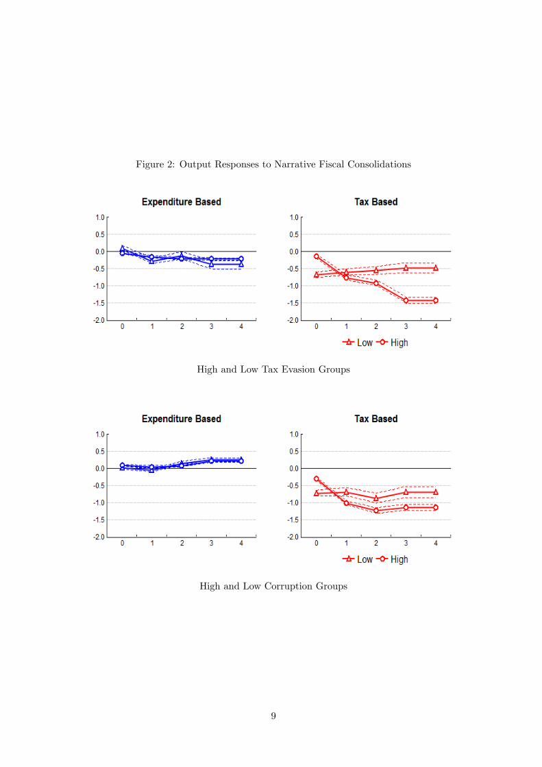
Figure 2: Output Responses to Narrative Fiscal Consolidations

High and Low Tax Evasion Groups

High and Low Corruption Groups

9

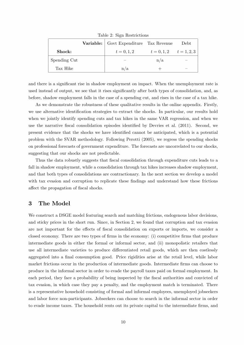
Table 2: Sign Restrictions

Variable: Govt Expenditure Tax Revenue Debt

Shock: t = 0; 1; 2 t = 0; 1; 2 t = 1; 2; 3

Spending Cut � n/a �

Tax Hike n/a + �

and there is a signi�cant rise in shadow employment on impact. When the unemployment rate is

used instead of output, we see that it rises signi�cantly after both types of consolidation, and, as

before, shadow employment falls in the case of a spending cut, and rises in the case of a tax hike.

As we demonstrate the robustness of these qualitative results in the online appendix. Firstly,

we use alternative identi�cation strategies to extract the shocks. In particular, our results hold

when we jointly identify spending cuts and tax hikes in the same VAR regression, and when we

use the narrative �scal consolidation episodes identi�ed by Devries et al. (2011). Second, we

present evidence that the shocks we have identi�ed cannot be anticipated, which is a potential

problem with the SVAR methodology. Following Perotti (2005), we regress the spending shocks

on professional forecasts of government expenditure. The forecasts are uncorrelated to our shocks,

suggesting that our shocks are not predictable.

Thus the data robustly suggests that �scal consolidation through expenditure cuts leads to a

fall in shadow employment, while a consolidation through tax hikes increases shadow employment,

and that both types of consolidations are contractionary. In the next section we develop a model

with tax evasion and corruption to replicate these �ndings and understand how these frictions

a¤ect the propagation of �scal shocks.

3 The Model

We construct a DSGE model featuring search and matching frictions, endogenous labor decisions,

and sticky prices in the short run. Since, in Section 2, we found that corruption and tax evasion

are not important for the e¤ects of �scal consolidation on exports or imports, we consider a

closed economy. There are two types of �rms in the economy: (i) competitive �rms that produce

intermediate goods in either the formal or informal sector, and (ii) monopolistic retailers that

use all intermediate varieties to produce di¤erentiated retail goods, which are then costlessly

aggregated into a �nal consumption good. Price rigidities arise at the retail level, while labor

market frictions occur in the production of intermediate goods. Intermediate �rms can choose to

produce in the informal sector in order to evade the payroll taxes paid on formal employment. In

each period, they face a probability of being inspected by the �scal authorities and convicted of

tax evasion, in which case they pay a penalty, and the employment match is terminated. There

is a representative household consisting of formal and informal employees, unemployed jobseekers

and labor force non-participants. Jobseekers can choose to search in the informal sector in order

to evade income taxes. The household rents out its private capital to the intermediate �rms, and

10

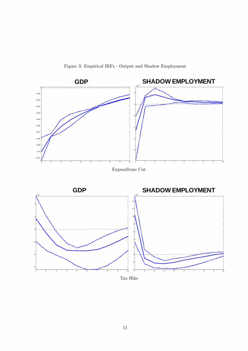
Figure 3: Empirical IRFs - Output and Shadow Employment

1 2 3 4 5 6 7 8 9 10

­0.011

­0.01

­0.009

­0.008

­0.007

­0.006

­0.005

­0.004

­0.003

­0.002

­0.001

0

GDP

1 2 3 4 5 6 7 8 9 10

­8

­6

­4

­2

0

2

x 10­4

SHADOW EMPLOYMENT

Expenditure Cut

1 2 3 4 5 6 7 8 9 10

­6

­4

­2

0

2

4

x 10­3

GDP

1 2 3 4 5 6 7 8 9 10­4

­2

0

2

4

6

8

10

12

14

x 10­4

SHADOW EMPLOYMENT

Tax Hike

11

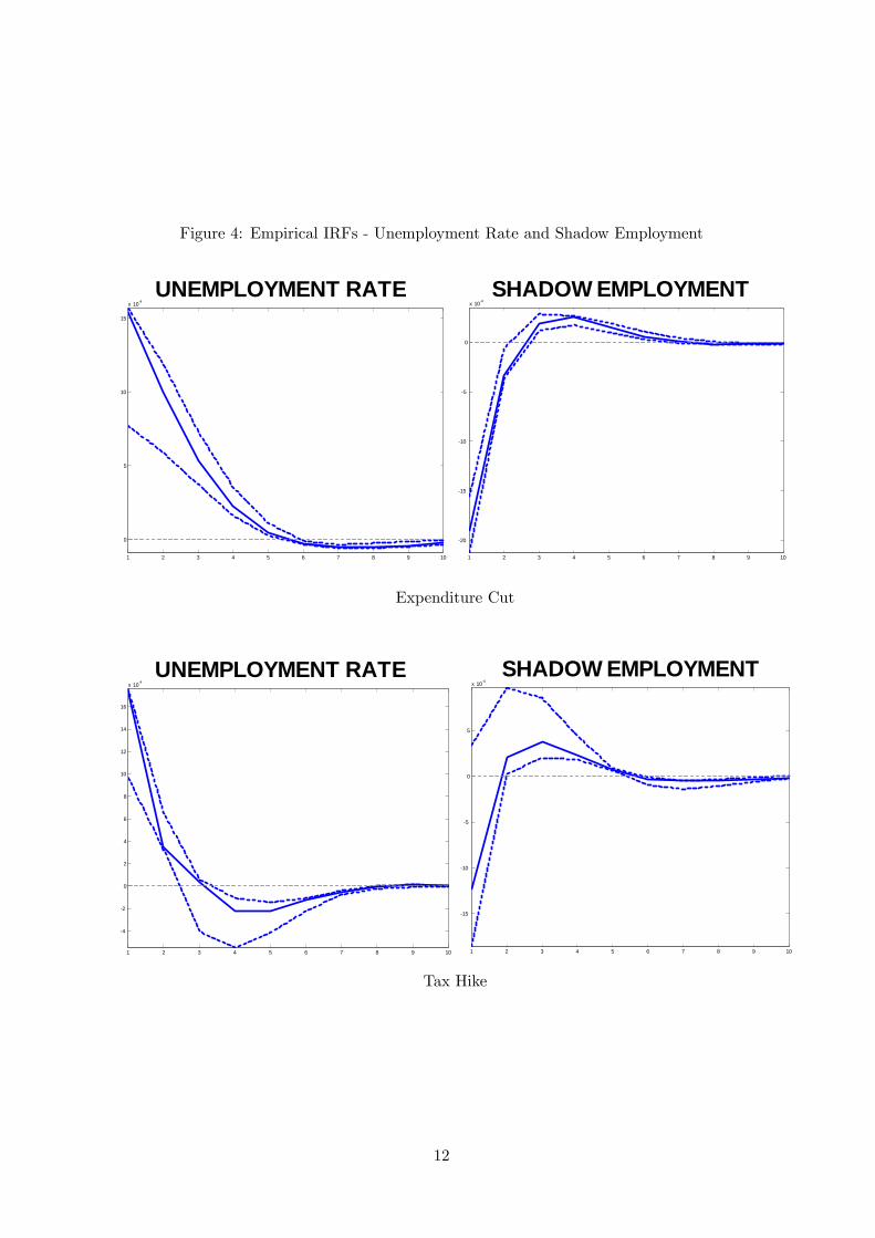
Figure 4: Empirical IRFs - Unemployment Rate and Shadow Employment

1 2 3 4 5 6 7 8 9 10

0

5

10

15

x 10­4UNEMPLOYMENT RATE

1 2 3 4 5 6 7 8 9 10

­20

­15

­10

­5

0

x 10­4SHADOW EMPLOYMENT

Expenditure Cut

1 2 3 4 5 6 7 8 9 10

­4

­2

0

2

4

6

8

10

12

14

16

x 10­4

UNEMPLOYMENT RATE

1 2 3 4 5 6 7 8 9 10

­15

­10

­5

0

5

x 10­4SHADOW EMPLOYMENT

Tax Hike

12

purchases the �nal consumption good. The government collects taxes from the regular sector,

embezzles a fraction of the revenues, and uses the remainder to �nance public expenditures and

the provision of unemployment bene�ts.

3.1 Labor markets

We account for the imperfections and transaction costs in the labor market by assuming that jobs

are created through a matching function. For j = F; I denoting the formal and informal sectors,

let �jt be the number of vacancies and ujt the number of jobseekers in each sector. We assume

matching functions of the form:

mjt = �j1(�

jt )�2(ujt )

1��2 (1)

where we allow for di¤erences in the e¢ ciency of the matching process, �j1, in the two sectors. In

each sector we can de�ne the probability of a jobseeker being hired, hjt , and of a vacancy being

�lled, fjt , as follows:

hjt � mjt

ujt; fjt � mj

t

�jt

In each period, jobs in the formal sector are destroyed at a constant fraction, �F , and mFt new

matches are formed. The law of motion of formal employment, nFt , is thus given by:

nFt+1 = (1� �F )nFt +mFt (2)

In the informal sector there is an exogenous fraction of jobs destroyed in each period, �I , as well

as a probability, �, that an informal employee loses their job due to an audit. The law of motion

of informal employment, nIt , is given by:

nIt+1 = (1� �� �I)nIt +mIt (3)

3.2 Households

The representative household consists of a continuum of in�nitely lived agents. The members of

the household derive utility from leisure, which corresponds to the fraction of members that are

out of the labor force, lt, and a consumption bundle, cct, de�ned as:

cct = [�1(ct)�2 + (1� �1)(gt)�2 ]

1�2

where gt denotes public consumption, taken as exogenous by the household, and ct is private

consumption. The elasticity of substitution between the private and public goods is given by

13

11��2 .

11 The instantaneous utility function is given by:

U(cct; lt) =cc1��t

1� � +�l1�'t

1� '

where � is the inverse of the intertemporal elasticity of substitution, � > 0 is the relative preference

for leisure, and ' is the inverse of the Frisch elasticity of labor supply.

At any point in time, a fraction nFt (nIt ) of the household members are formal (informal)

employees. Campolmi and Gnocchi (2014), Brückner and Pappa (2012) and Bermperoglou et

al. (2014) have added a labor force participation choice in New Keynesian models of equilibrium

unemployment. Following Ravn (2008), the participation choice is modelled as a trade-o¤between

the cost of giving up leisure and the prospect of �nding a job. In particular, the household chooses

the fraction of the unemployed actively searching for a job, ut, and the fraction which are out of

the labor force and enjoying leisure, lt, so that:

nFt + nIt + ut + lt = 1 (4)

The household chooses the fraction of jobseekers searching in each sector: a share st of jobseekers

look for a job in the informal sector, while the remainder, (1� st), seek employment in the formalsector. That is, uIt � stut and uFt � (1� st)ut.

The household owns the capital stock, which evolves over time according to:

kt+1 = it + (1� �)kt �!

2

�kt+1kt

� 1�2

kt (5)

where it is investment, � is a constant depreciation rate and !2

�kt+1kt� 1�2kt are adjustment costs.

The intertemporal budget constraint is given by:

(1 + � ct)ct + it +Bt+1�t+1

Rt� rtkt + (1� �nt )wFt nFt + wIt nIt +$uFt +Bt +�

pt � Tt (6)

where �t � pt=pt�1 is the gross in�ation rate, wjt ; j = F; I, are the real wages in the two sectors, rt

is the real return on capital, $ denotes unemployment bene�ts, available only to formal jobseekers

(see e.g. Boeri and Garibaldi, 2007), Bt is the real government bond holdings, Rt is the gross

nominal interest rate, �pt are the pro�ts of the monopolistic retailers, discussed below, and �ct , �

nt

and Tt represent taxes on private consumption, labor income and lump-sum taxes respectively.

The household maximizes expected lifetime utility subject to (1) for each j, (2), (3), (4), (5),

and (6). Taking as given njt , they choose ut, st (which together determine lt) and njt+1, as well as

ct, kt+1 and Bt+1.

It is convenient to de�ne the marginal value to the household of having an additional member

11When �2 approaches one, ct and gt are perfect substitutes. They are instead perfect complements if �2 tendsto minus in�nity. �2 = 0 nests the Cobb-Douglas speci�cation.

14

employed in each sector, as follows:

V hnF t = �ctwFt (1� �nt )� �l

�'t + (1� �F )�nF t (7)

V hnI t = �ctwIt � �l

�'t + (1� �� �I)�nI t (8)

where �nF t, �nI t and �ct are the multipliers in front of (2), (3) and (6) respectively.12

3.3 Production

3.3.1 Intermediate goods �rms

Intermediate goods are produced with two di¤erent technologies:

xFt = (AFt n

Ft )1��F (kt)

�F (9)

xIt = (AItnIt )1��I (10)

where Ajt denotes total factor productivity in sector j. Following the literature, we assume that

the informal production technology uses labor inputs only (see e.g. Busato and Chiarini, 2004).

Firms maximize the discounted value of future pro�ts, subject to (2) and (3). That is, they

take the number of workers currently employed in each sector, njt ; as given and choose the number

of vacancies posted in each sector, �jt , so as to employ the desired number of workers next period,

njt+1. Here, �rms adjust employment by varying the number of workers (extensive margin) rather

than the number of hours per worker (intensive margin). According to Hansen (1985), most of

the employment �uctuations arise from movements in this margin. Firms also decide the amount

of private capital, kt, needed for production. They face a probability, �, of being inspected by

the �scal authorities, convicted of tax evasion and forced to pay a penalty, which is a fraction,

, of their total revenues. We assume that, once they are produced, there is no di¤erentiation

between intermediate goods from the di¤erent sectors. In other words, we assume that formal and

informal goods are perfect substitutes, so that they are sold at the same price, pxt (see e.g. Orsi

et al., 2014). Hence the problem of an intermediate �rm is summarized by the following Bellman

equation:

Q(nFt ; nIt ) = max

kt;�Ft ;�It

n(1� � ) pxt (xFt + xIt )� (1 + � st )wFt nFt � wIt nIt � rtkt

� �F�Ft � �I�It + Et��t;t+1Q(n

Ft+1; n

It+1)

� owhere � st is a payroll tax, �

j is the cost of posting a new vacancy in sector j, and �t;t+1 ��Ucc;t+1Ucc;t

= ��cct+1cct

���is a discount factor. The �rst-order conditions are:

rt = (1� � ) pxt��FxFtkt

�(11)

12The �rst order conditions of the household�s problem and the derivations of equations (7) and (8) are presentedin the online appendix.

15

�F

fFt= Et�t;t+1

"(1� � ) pxt+1(1� �F )

xFt+1nFt+1

� (1 + � st+1)wFt+1 +(1� �F )�F

fFt+1

#(12)

�I

fIt= Et�t;t+1

"(1� � ) pxt+1(1� �I)

xIt+1nIt+1

� wIt+1 +(1� �� �I)�I

fIt+1

#(13)

According to (11)-(13), the net value of the marginal product of private capital should equal the

real rental rate and the expected marginal cost of hiring a worker in each sector j should equal

the expected marginal bene�t. The latter includes the net value of the marginal product of labor

minus the wage, augmented by the payroll tax in the formal sector, plus the continuation value.

For convenience, we de�ne the value of the marginal formal and informal job for the interme-

diate �rm:

V fnF t

= (1� � ) pxt (1� �F )xFtnFt

� (1 + � st )wFt +(1� �F )�F

fFt(14)

V fnI t= (1� � ) pxt (1� �I)

xItnIt� wIt +

(1� �� �I)�I

fIt(15)

3.3.2 Retailers

There is a continuum of monopolistically competitive retailers indexed by i on the unit interval.

Retailers buy intermediate goods and di¤erentiate them with a technology that transforms one

unit of intermediate goods into one unit of retail goods, and thus the relative price of intermediate

goods, pxt , coincides with the real marginal cost faced by the retailers. Let yit be the quantity of

output sold by retailer i. The �nal consumption good can be expressed as:

yt =

�Z 1

0(yit)

��1� di

� ���1

(16)

where � > 1 is the constant elasticity of demand for retail goods. The �nal good is sold at a price

pt =hR 10 p

1��it di

i 11��. The demand for each intermediate good depends on its relative price and on

aggregate demand:

yit =

�pitpt

���yt (17)

Following Calvo (1983), we assume that in any given period each retailer can reset its price with

a �xed probability (1� �). Hence, the price index is given by:

pt =�(1� �)(p�t )1�� + �(pt�1)1��

� 11�� (18)

Firms that are able to reset their price choose p�it so as to maximize expected pro�ts given by:

Et

1Xs=0

�s�t;t+s(p�it � pxt+s)yit+s

16

The resulting expression for p�it is:

p�it =�

�� 1EtP1s=0 �

s�t;t+spxt+syit+s

EtP1s=0 �

s�t;t+syit+s(19)

3.4 Government

Government expenditure consists of consumption purchases and unemployment bene�ts, while

revenues come from the collected �nes and the payroll, consumption, and labor income taxes, as

well as the lump-sum taxes. The government de�cit is therefore de�ned by:

DFt = gt +$uFt � (1� �TR)TRt � � pxt (xFt + xIt ) (20)

where TRt � (�nt + � st )wFt n

Ft + � ctct + Tt denotes tax revenues and �TR 2 [0; 1) denotes the

embezzlement rate in the presence of corruption in the economy.

The government budget constraint is given by:

Bt +DFt = R�1t Bt+1�t+1 (21)

We assume that Tt; � st ; and �ct are constant and �xed at their steady state levels, and we do not

consider them as active instruments for �scal consolidation. In our model, the e¤ects of payroll

taxes are very similar to labor income taxes. Consumption taxes can have di¤erent e¤ects, but

they generally constitute a relatively small source of tax revenues. Thus, in line with Erceg and

Lindé (2013), the government has two potential �scal instruments, g and �n. We consider each

instrument separately, assuming that if one is active, the other remains �xed at its steady state

value. For 2 fg; �ng, we assume �scal rules of the form:

t = (1��0)

�0t�1 expf(1� �0)[�1(bt � b�t ) + �2(�bt+1 ��b�t+1)]g (22)

where bt = Btytis the debt-to-GDP ratio, and b�t is the target value for this ratio, given by the

AR(2) process:

log b�t+1 � log b�t = �b + �1(log b�t � log b�t�1)� �2 log b�t � "bt (23)

where "bt is a white noise shock representing a �scal consolidation.

3.5 Closing the model

Monetary Policy There is an independent monetary authority that sets the nominal interest

rate as a function of current in�ation according to the rule:

Rt = R expf��(�t � 1)g (24)

where R is the steady state value of the nominal interest rate.

17

Goods Markets Total output must equal private and public demand. The aggregate resource

constraint is thus given by:

yt = ct + it + gt + �F�Ft + �

I�It + �TRTRt (25)

where the last term is the resource cost of corruption in the economy.13

The aggregate price index, pt, is given by (18) and (19). The return on private capital, rt,

adjusts so that the capital demanded by the intermediate goods �rm, given by (11), is equal to

the stock held by the household.

Bargaining over wages Wages in both sectors are determined by ex-post (after matching)

Nash bargaining. Workers and �rms split rents and the part of the surplus they receive depends

on their bargaining power. We denote by #j 2 (0; 1) the �rms�bargaining power in sector j. TheNash bargaining problem is to maximize the weighted sum of log surpluses:

maxwjt

n(1� #j) log V hnjt + #

j log V fnjt

owhere V h

njtand V f

njtare de�ned in equations (7), (8), (14) and (15). As shown in the online

appendix, wages are given by:

wFt =(1� #F )(1 + � st )

(1� � ) pxt (1� �F )

xFtnFt

+(1� �F )�F

fFt

!+

#F

�ct(1� �nt )

��l�'t �(1��F )�nF t

�(26)

wIt = (1�#I) (1� � ) pxt (1� �I)

xItnIt+(1� �� �I)�I

fIt

!+#I

�ct

��l�'t � (1����I)�nI t

�(27)

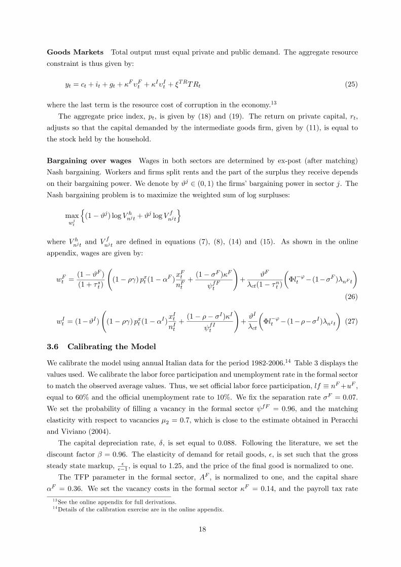
3.6 Calibrating the Model

We calibrate the model using annual Italian data for the period 1982-2006.14 Table 3 displays the

values used. We calibrate the labor force participation and unemployment rate in the formal sector

to match the observed average values. Thus, we set o¢ cial labor force participation, lf � nF+uF ,

equal to 60% and the o¢ cial unemployment rate to 10%. We �x the separation rate �F = 0:07.

We set the probability of �lling a vacancy in the formal sector fF = 0:96, and the matching

elasticity with respect to vacancies �2 = 0:7, which is close to the estimate obtained in Peracchi

and Viviano (2004).

The capital depreciation rate, �, is set equal to 0:088. Following the literature, we set the

discount factor � = 0:96. The elasticity of demand for retail goods, �, is set such that the gross

steady state markup, ���1 , is equal to 1:25, and the price of the �nal good is normalized to one.

The TFP parameter in the formal sector, AF , is normalized to one, and the capital share

�F = 0:36. We set the vacancy costs in the formal sector �F = 0:14; and the payroll tax rate

13See the online appendix for full derivations.14Details of the calibration exercise are in the online appendix.

18

Table 3: Calibration ValuesParameter Description Full Model

� Discount Factor 0.96� Depreciation Rate 0.088�1 Share of Private Consumption in Utility 1� Inverse Elasticity of Intertemporal Substitution 2' Inverse Frisch Elasticity of Labor Supply 2� Relative Utility from Leisure 0.7lf O¢ cial Labor Force Participation 0.6uF

lf O¢ cial Unemployment Rate 0.1u1�l Actual Unemployment Rate 0.09s Share of Informal Jobseekers to Total 0.10nI

n Share of Informal Employment to Total 0.13�F Exogenous Job Destruction Rate - Formal Sector 0.07�I Exogenous Job Destruction Rate - Informal Sector 0.0545� Auditing Probability 0.02�F1 Matching E¢ ciency - Formal Sector 0.85�I1 Matching E¢ ciency - Informal Sector 0.12�2 Elasticity of Matching to Vacancies 0.7 fF Probability of Filling a Vacancy - Formal Sector 0.96 fI Probability of Filling a Vacancy - Informal Sector 0.05 hF Probability of Finding a Job - Formal Sector 0.63 hI Probability of Finding a Job - Informal Sector 0.91AF TFP - Formal Sector 1AI TFP - Informal Sector 0.6�F Capital Share - Formal Sector 0.36�I Production Function Parameter - Informal Sector 0.4yI

y Share of Underground Output in Total 0.16�F Vacancy Costs - Formal Sector 0.14�F

wFVacancy Costs/Wage 0.21

�I Vacancy Costs - Informal Sector 0.13� Price Elasticity of Demand 5#F Firm�s Bargaining Power - Formal Sector 0.22#I Firm�s Bargaining Power - Informal Sector 0.80wI

wFFormal/Informal Wage Di¤erentials 0.98

gy Government Expenditure-to-GDP Ratio 0.11$wF

Replacement Rate 0.35�n Labor Income Tax Rate 0.4� s Payroll Tax Rate 0.16� c Consumption Tax Rate 0.18 Proportional Fine in Case of Auditing 0.3�TR Embezzlement Rate 0.2DFy De�cit-to-GDP Ratio -0.04b Debt-to-GDP Ratio 1.03

�1, �2 Debt-to-GDP Target Parameters 0.85, 0.0001� Price Stickiness 0.25! Capital Adjustment Costs 0.5�� Taylor Rule Parameter 1.5

19

� s = 16%, close to the value used in Orsi et al. (2014).

In the informal sector, we assume that TFP is lower than the formal sector by setting AI = 0:6.

According to Restrepo-Echavarria (2014), the fact that the informal sector has restricted access

to credit leads to fewer resources being devoted to research and development, or to absorbing

technology spillovers, which in turn reduces productivity. Also, both Boeri and Garibaldi (2007)

and Orsi et al. (2014) emphasize empirical evidence suggesting that the workers in the informal

sector have lower education levels.15

Using the ISTAT data, we set the share of informal employment to total employment equal

to 0:13; and we set �I = 0:4, implying the share of shadow output to total output yI

y = 16%.

We set the exogenous job destruction rate in the informal sector �I = 0:0545, the probability of

�lling a vacancy in the informal sector fI = 0:05, and the vacancy cost in the informal sector

�I = 0:13. These values yield a relatively small wage premium for the formal sector, wI

wF= 0:98,

in line with the literature. The probability of audit and the fraction of total revenues paid as a

�ne in the event of an audit are set as follows: � = 0:02, close to the value used in Boeri and

Garibaldi (2007), and = 0:3.

We set the replacement rate $wF

= 0:35, close to the estimates in Martin (1996), and used by

Fugazza and Jacques (2004). Government spending as a share of GDP and the remaining tax

rates are set as follows: gy = 11%, �

n = 40%, in line with Orsi et al. (2014), and � c = 18%. The

steady state debt-to-GDP ratio b = 103%. We set the corruption parameter �TR = 0:2.

We begin by assuming purely wasteful government expenditure, setting �1 = 1, and will

consider utility enhancing government spending as an extension. Regarding the inverse elasticity

of intertemporal substitution, �, much of the literature cites the econometric estimates of Hansen

and Singleton (1983), which place it �between 0 and 2�, and often choose a value greater than

unity. In our calibration, we set � = 2 and we perform sensitivity analysis by considering � equal

to 0.5 and 1. The inverse of the Frisch elasticity, ', is set equal to 2. Finally, we set the in�ation

targeting parameter in the Taylor rule �� = 1:5, the capital adjustment costs ! = 0:5 and the

price-stickiness parameter � = 0:25.

3.7 Results

We present responses following a negative debt-target shock (following Erceg and Lindé, 2013).

We compare the e¤ects of a 5% reduction in the desired long run debt target, which is achieved

after 10 years, either through a fall in government consumption expenditure, or a hike in labor

tax rates.16

3.7.1 Dynamics in a Model Without Tax Evasion and Corruption

As a benchmark, we begin by analyzing the responses of a standard model where tax evasion and

corruption are absent, shown in Figure 5.

15Orsi et al. (2014) also note the equivalence of assuming lower productivity in the informal sector to assuminga cost for concealing production.16For comparison purposes, throughout this section we adjust the parameters of the policy rules for each case to

ensure that the debt target is met after 10 years.

20

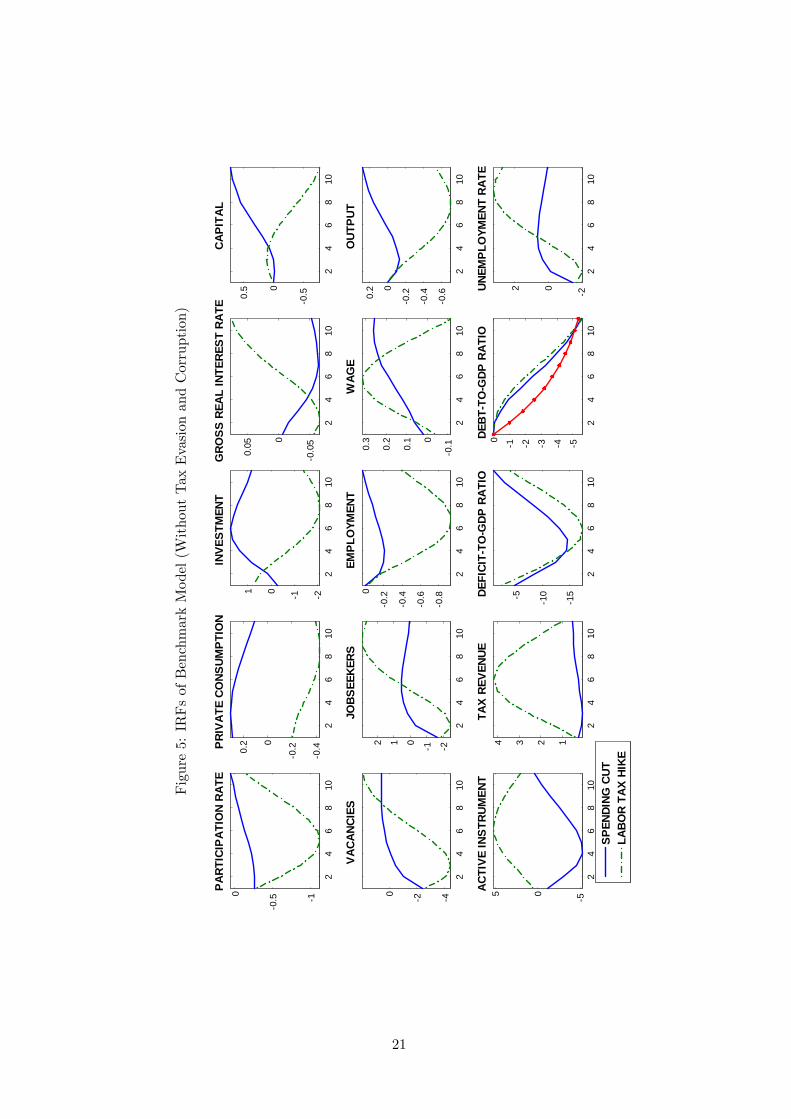
Figure5:IRFsofBenchmarkModel(WithoutTaxEvasionandCorruption)

24

68

10

­1

­0.50PA

RTIC

IPAT

ION 

RATE

24

68

10­0

.4

­0.20

0.2PR

IVAT

E CO

NSUM

PTIO

N

24

68

10­2­101

INVE

STM

ENT

24

68

10

­0.0

50

0.05

GRO

SS R

EAL 

INTE

REST

 RAT

E

24

68

10

­0.50

0.5

CAPI

TAL

24

68

10­4­20

VACA

NCIE

S

24

68

10­2­1012

JOBS

EEKE

RS

24

68

10

­0.8

­0.6

­0.4

­0.20

EMPL

OYM

ENT

24

68

10­0

.10

0.1

0.2

0.3

WAG

E

24

68

10

­0.6

­0.4

­0.20

0.2

OUT

PUT

24

68

10­505AC

TIVE

 INST

RUM

ENT

24

68

10

1234TA

X RE

VENU

E

24

68

10

­15

­10­5DE

FICI

T­TO

­GDP

 RAT

IO

24

68

10

­5­4­3­2­10DEBT

­TO

­GDP

 RAT

IO

24

68

10­202UN

EMPL

OYM

ENT 

RATE

SPEN

DING

 CUT

LABO

R TA

X HI

KE

21

A consolidation carried out through a fall in government spending has two e¤ects. Firstly,

there is a negative demand e¤ect for �rms, which leads, in the presence of nominal rigidities, to

a fall in labor demand and hence in vacancies. Second, there is a positive wealth e¤ect for the

household, which increases consumption and investment and reduces labor force participation.

Given the drop in both labor demand and supply, employment falls and the wage rate rises.

Output falls in the short run, but increases in the medium and long run because investment, and

hence the capital stock, increases. The unemployment rate re�ects movements in the number of

jobseekers: it falls on impact, but then increases as employment and wages adjust.

When the �scal consolidation is carried out through a labor tax hike, there is a negative wealth

e¤ect for the household which makes consumption fall, and investment fall with a lag. However,

as the return from employment falls, there is a substitution e¤ect which outweighs the wealth

e¤ect, and leads to a decrease in labor force participation. The fall in private demand induces

�rms to contract their labor demand, again expressed through a drop in vacancies. Employment

and output fall, and the responses are signi�cantly larger and more persistent than in the case of

spending cuts, due to the fall in investment.

Thus, our benchmark model seems to be consistent with the evidence of Alesina et al. (2013):

spending cuts are accompanied by mild and short-lived recessions, while tax hikes lead to more

prolonged and deep recessions.

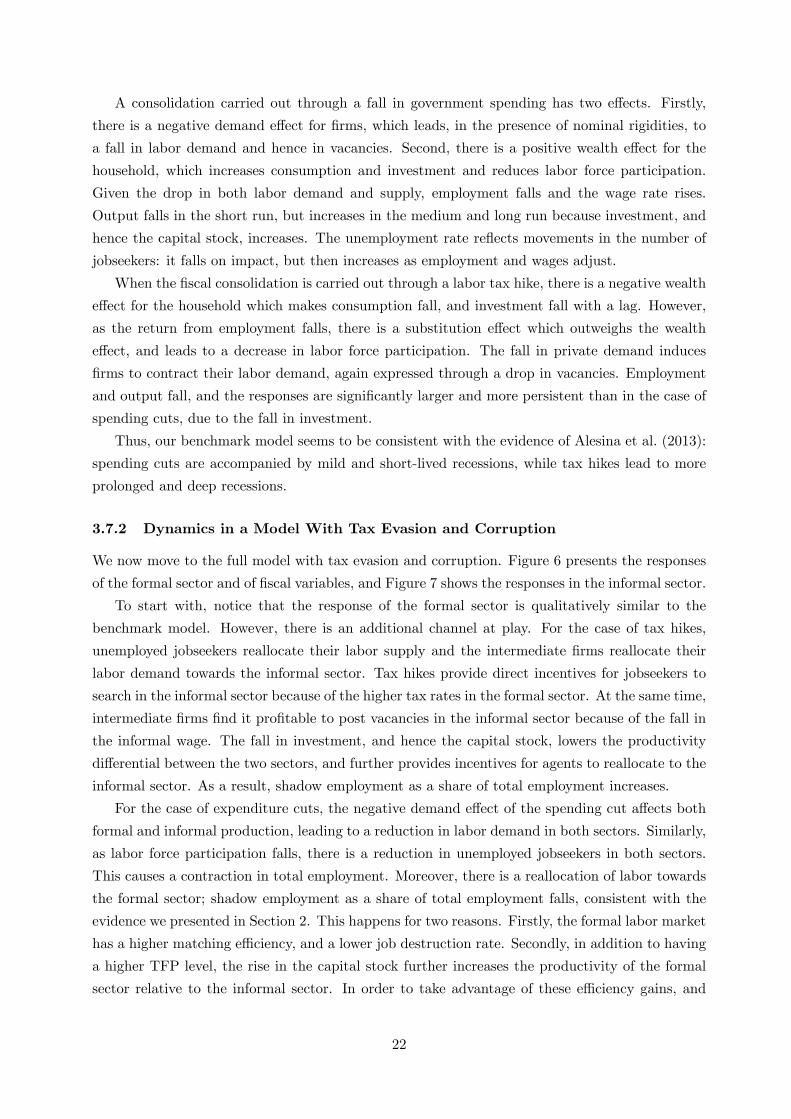
3.7.2 Dynamics in a Model With Tax Evasion and Corruption

We now move to the full model with tax evasion and corruption. Figure 6 presents the responses

of the formal sector and of �scal variables, and Figure 7 shows the responses in the informal sector.

To start with, notice that the response of the formal sector is qualitatively similar to the

benchmark model. However, there is an additional channel at play. For the case of tax hikes,

unemployed jobseekers reallocate their labor supply and the intermediate �rms reallocate their

labor demand towards the informal sector. Tax hikes provide direct incentives for jobseekers to

search in the informal sector because of the higher tax rates in the formal sector. At the same time,

intermediate �rms �nd it pro�table to post vacancies in the informal sector because of the fall in

the informal wage. The fall in investment, and hence the capital stock, lowers the productivity

di¤erential between the two sectors, and further provides incentives for agents to reallocate to the

informal sector. As a result, shadow employment as a share of total employment increases.

For the case of expenditure cuts, the negative demand e¤ect of the spending cut a¤ects both

formal and informal production, leading to a reduction in labor demand in both sectors. Similarly,

as labor force participation falls, there is a reduction in unemployed jobseekers in both sectors.

This causes a contraction in total employment. Moreover, there is a reallocation of labor towards

the formal sector; shadow employment as a share of total employment falls, consistent with the

evidence we presented in Section 2. This happens for two reasons. Firstly, the formal labor market

has a higher matching e¢ ciency, and a lower job destruction rate. Secondly, in addition to having

a higher TFP level, the rise in the capital stock further increases the productivity of the formal

sector relative to the informal sector. In order to take advantage of these e¢ ciency gains, and

22

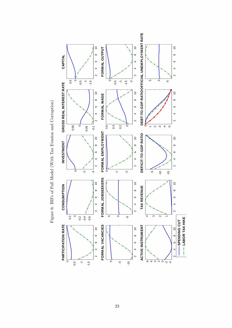
Figure6:IRFsofFullModel(WithTaxEvasionandCorruption)

24

68

10

­1.5­1

­0.50PA

RTI

CIP

ATIO

N R

ATE

24

68

10

­0.6

­0.4

­0.20

0.2

CO

NSU

MPT

ION

24

68

10­4­20

INVE

STM

ENT

24

68

10­0

.1

­0.0

50

0.05

GR

OSS

 REA

L IN

TER

EST 

RAT

E

24

68

10

­1.5­1

­0.50

0.5

CAP

ITAL

24

68

10

­10­50FO

RM

AL V

ACAN

CIE

S

24

68

10

­505FOR

MAL

 JO

BSE

EKER

S

24

68

10

­2­10FOR

MAL

 EM

PLO

YM

ENT

24

68

10

0

0.2

0.4

0.6

FOR

MAL

 WAG

E

24

68

10­2

­1.5­1

­0.50

FOR

MAL

 OU

TPU

T

24

68

10­4­202468AC

TIVE

 INST

RU

MEN

T

24

68

10

1234

TAX 

REV

ENU

E

24

68

10

­15

­10­5D

EFIC

IT­T

O­G

DP 

RAT

IO

24

68

10

­5­4­3­2­10DEB

T­TO

­GD

P R

ATIO

24

68

10

­505

OFF

ICIA

L U

NEM

PLO

YM

ENT 

RAT

E

SPEN

DIN

G C

UT

LAB

OR

 TAX

 HIK

E

23

Figure7:IRFsofFullModel-UndergroundSector

24

68

10­1

00102030

UN

DER

GR

OU

ND

 VAC

ANC

IES

24

68

10

0102030

UN

DER

GR

OU

ND

 JO

BSE

EKER

S

24

68

10­3

.5­3

­2.5­2

­1.5­1

­0.50

UN

DER

GR

OU

ND

 WAG

E

24

68

1002468

SHAR

E O

F U

ND

ERG

RO

UN

D E

MPL

OY

MEN

T

24

68

10

01234

UN

DER

GR

OU

ND

 OU

TPU

T

SPEN

DIN

G C

UT

LAB

OR

 TAX

 HIK

E

24

thus mitigate the negative e¤ects of the �scal contraction, agents optimally choose to reallocate

towards the formal sector.17

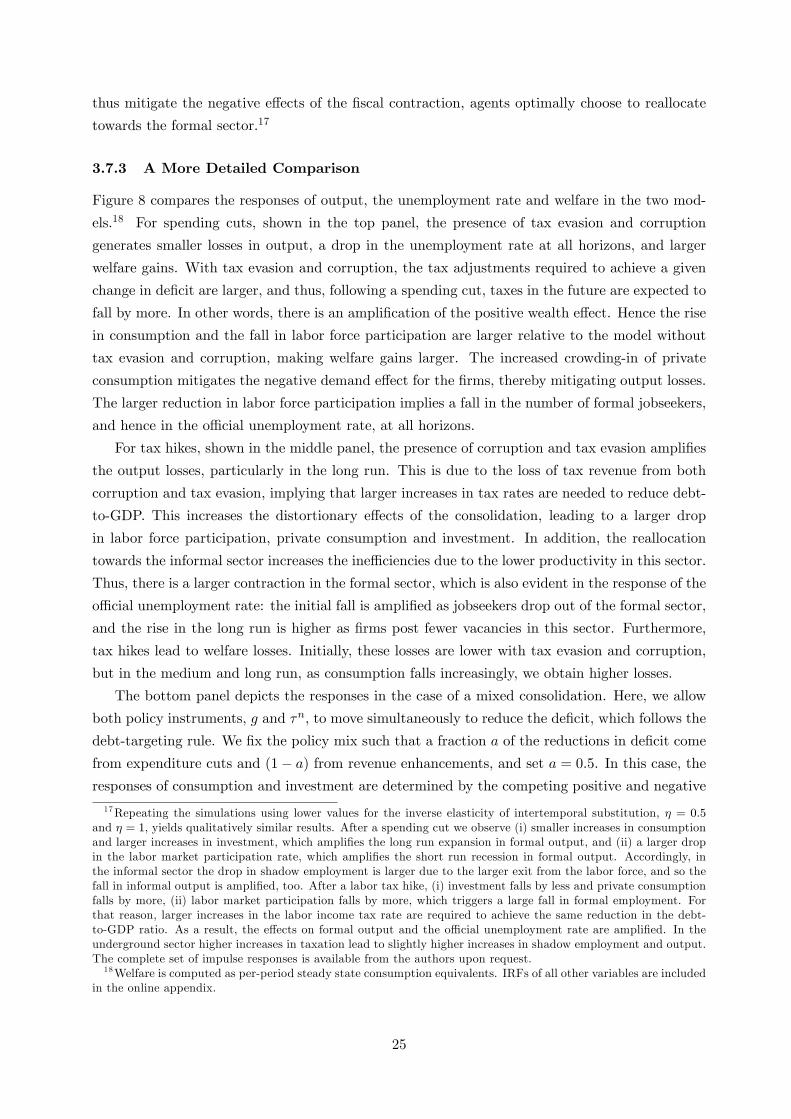
3.7.3 A More Detailed Comparison

Figure 8 compares the responses of output, the unemployment rate and welfare in the two mod-

els.18 For spending cuts, shown in the top panel, the presence of tax evasion and corruption

generates smaller losses in output, a drop in the unemployment rate at all horizons, and larger

welfare gains. With tax evasion and corruption, the tax adjustments required to achieve a given

change in de�cit are larger, and thus, following a spending cut, taxes in the future are expected to

fall by more. In other words, there is an ampli�cation of the positive wealth e¤ect. Hence the rise

in consumption and the fall in labor force participation are larger relative to the model without

tax evasion and corruption, making welfare gains larger. The increased crowding-in of private

consumption mitigates the negative demand e¤ect for the �rms, thereby mitigating output losses.

The larger reduction in labor force participation implies a fall in the number of formal jobseekers,

and hence in the o¢ cial unemployment rate, at all horizons.

For tax hikes, shown in the middle panel, the presence of corruption and tax evasion ampli�es

the output losses, particularly in the long run. This is due to the loss of tax revenue from both

corruption and tax evasion, implying that larger increases in tax rates are needed to reduce debt-

to-GDP. This increases the distortionary e¤ects of the consolidation, leading to a larger drop

in labor force participation, private consumption and investment. In addition, the reallocation

towards the informal sector increases the ine¢ ciencies due to the lower productivity in this sector.

Thus, there is a larger contraction in the formal sector, which is also evident in the response of the

o¢ cial unemployment rate: the initial fall is ampli�ed as jobseekers drop out of the formal sector,

and the rise in the long run is higher as �rms post fewer vacancies in this sector. Furthermore,

tax hikes lead to welfare losses. Initially, these losses are lower with tax evasion and corruption,

but in the medium and long run, as consumption falls increasingly, we obtain higher losses.

The bottom panel depicts the responses in the case of a mixed consolidation. Here, we allow

both policy instruments, g and �n, to move simultaneously to reduce the de�cit, which follows the

debt-targeting rule. We �x the policy mix such that a fraction a of the reductions in de�cit come

from expenditure cuts and (1� a) from revenue enhancements, and set a = 0:5. In this case, the

responses of consumption and investment are determined by the competing positive and negative

17Repeating the simulations using lower values for the inverse elasticity of intertemporal substitution, � = 0:5and � = 1, yields qualitatively similar results. After a spending cut we observe (i) smaller increases in consumptionand larger increases in investment, which ampli�es the long run expansion in formal output, and (ii) a larger dropin the labor market participation rate, which ampli�es the short run recession in formal output. Accordingly, inthe informal sector the drop in shadow employment is larger due to the larger exit from the labor force, and so thefall in informal output is ampli�ed, too. After a labor tax hike, (i) investment falls by less and private consumptionfalls by more, (ii) labor market participation falls by more, which triggers a large fall in formal employment. Forthat reason, larger increases in the labor income tax rate are required to achieve the same reduction in the debt-to-GDP ratio. As a result, the e¤ects on formal output and the o¢ cial unemployment rate are ampli�ed. In theunderground sector higher increases in taxation lead to slightly higher increases in shadow employment and output.The complete set of impulse responses is available from the authors upon request.18Welfare is computed as per-period steady state consumption equivalents. IRFs of all other variables are included

in the online appendix.

25

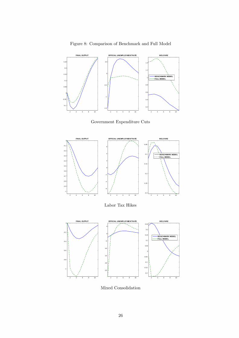
Figure 8: Comparison of Benchmark and Full Model

2 4 6 8 10

­0.1

­0.05

0

0.05

0.1

0.15

0.2

0.25

FINAL OUTPUT

2 4 6 8 10

­1.5

­1

­0.5

0

0.5

OFFICIAL UNEMPLOYMENT RATE

2 4 6 8 10

0.2

0.4

0.6

0.8

1

1.2

1.4

WELFARE

BENCHMARK MODELFULL MODEL

Government Expenditure Cuts

2 4 6 8 10

­1

­0.9

­0.8

­0.7

­0.6

­0.5

­0.4

­0.3

­0.2

­0.1

0FINAL OUTPUT

2 4 6 8 10

­6

­4

­2

0

2

4

6

OFFICIAL UNEMPLOYMENT RATE

2 4 6 8 10­0.3

­0.25

­0.2

­0.15

­0.1

­0.05

WELFARE

BENCHMARK MODELFULL MODEL

Labor Tax Hikes

2 4 6 8 10

­1

­0.8

­0.6

­0.4

­0.2

0FINAL OUTPUT

2 4 6 8 10

­25

­20

­15

­10

­5

0

5

OFFICIAL UNEMPLOYMENT RATE

2 4 6 8 10

­0.2

­0.15

­0.1

­0.05

0

0.05

0.1

0.15

0.2

0.25

WELFARE

BENCHMARK MODELFULL MODEL

Mixed Consolidation

26

wealth e¤ects from the two instruments, and the presence of tax evasion and corruption plays an

important role in determining this relative strength. In the benchmark model, the positive wealth

e¤ect of the expenditure cut is dominant and consumption rises for several periods. When there

is tax evasion and corruption, this is no longer true and consumption and investment fall in all

periods. Hence, as in the case of tax hikes, output and unemployment responses are ampli�ed

in the presence of tax evasion and corruption. This is in line with the BL (2013) regressions

presented in Section 2. Moreover, the welfare gains obtained from mixed consolidation packages

in the benchmark model turn into welfare losses in the model with tax evasion and corruption.

3.7.4 Sensitivity Analysis

While the e¤ects of labor tax hikes are robust to variations in a number of parameters, the e¤ects

of expenditure cuts depend crucially on some modeling assumptions. For instance, assuming that

government expenditures provide a public good, which is consumed by households, can change the

welfare implications of spending cuts. To illustrate this point, we set �1 = 0:85 and �2 = �0:25,so that private and public spending are weak complements. Figure 9 compares the results of this

case with those obtained with wasteful government spending. In the case of utility enhancing

expenditures, a spending cut directly reduces the consumption bundle, and households are forced

to o¤set this fall by further increasing private consumption. Thus we see a larger crowding-in

of private consumption, which mitigates the output and unemployment e¤ects of spending cuts.

However, the welfare e¤ects are reversed: the drop in the consumption bundle causes welfare to

fall for several periods.

The presence of liquidity constrained consumers has been shown to play an important role in

determining the response of private consumption to a government spending cut (see Galí et al.,

2007). To explore how the presence of liquidity constrained consumers can a¤ect our model, we

assume a fraction of rule of thumb (ROT) household members, which we set equal to 44%, in

line with the Italian household survey reported by Martin and Philippon (2014). As shown in the

bottom panel of Figure 9, output and unemployment responses are ampli�ed and welfare gains

are mitigated following a spending cut. The presence of ROT agents reduces the positive wealth

e¤ect that the �scal contraction generates, which implies a smaller increase in consumption and,

hence, welfare, and a larger contraction in output.

4 Policy Evaluation

Since the model qualitatively replicates the empirical evidence presented in Section 2, we employ

it to evaluate the e¤ects of consolidation packages implemented in Southern European countries

in recent years. We recalibrate the model for Greece, Portugal and Spain, three countries which

are also characterized by high corruption and tax evasion, and analyze the e¤ects of their recent

consolidation packages.

Using the information in OECD (2012), we adjust the size of the consolidation in each country

to match the reduction in the de�cit-to-GDP ratio implemented in 2010 and also replicate the

27

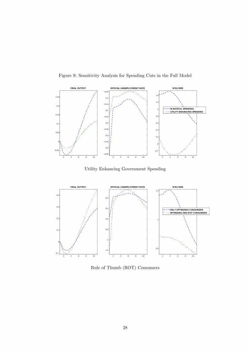
Figure 9: Sensitivity Analysis for Spending Cuts in the Full Model

2 4 6 8 10

­0.05

0

0.05

0.1

0.15

0.2

0.25

FINAL OUTPUT

2 4 6 8 10

­0.55

­0.5

­0.45

­0.4

­0.35

­0.3

­0.25

­0.2

­0.15

­0.1

­0.05

OFFICIAL UNEMPLOYMENT RATE

2 4 6 8 10

­0.2

0

0.2

0.4

0.6

0.8

1

1.2

1.4

W ELFARE

W ASTEFUL SPENDINGUTILITY ENHANCING SPENDING

Utility Enhancing Government Spending

2 4 6 8 10­0.1

0

0.1

0.2

0.3

0.4

FINAL OUTPUT

2 4 6 8 10

­1.2

­1

­0.8

­0.6

­0.4

­0.2

OFFICIAL UNEMPLOYMENT RATE

2 4 6 8 10

0.5

1

1.5

W ELFARE

ONLY OPTIMIZING CONSUMERSOPTIMIZING AND ROT CONSUMERS

Rule of Thumb (ROT) Consumers

28

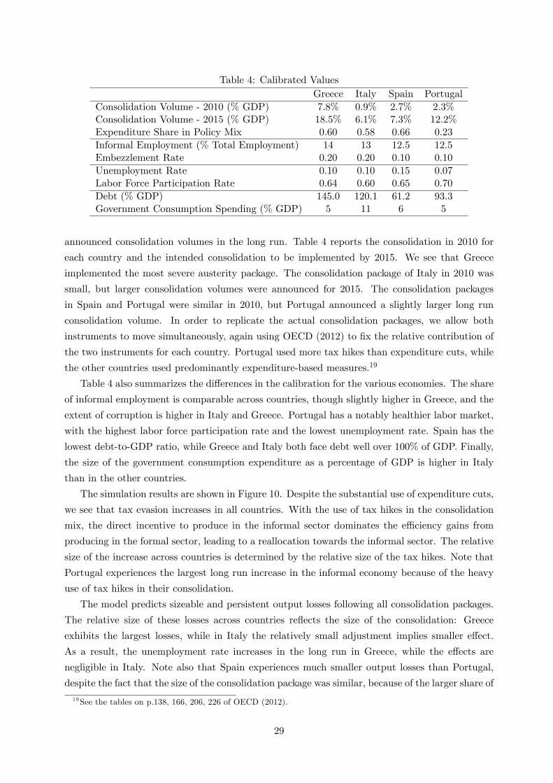
Table 4: Calibrated ValuesGreece Italy Spain Portugal

Consolidation Volume - 2010 (% GDP) 7.8% 0.9% 2.7% 2.3%Consolidation Volume - 2015 (% GDP) 18.5% 6.1% 7.3% 12.2%Expenditure Share in Policy Mix 0.60 0.58 0.66 0.23Informal Employment (% Total Employment) 14 13 12.5 12.5Embezzlement Rate 0.20 0.20 0.10 0.10Unemployment Rate 0.10 0.10 0.15 0.07Labor Force Participation Rate 0.64 0.60 0.65 0.70Debt (% GDP) 145.0 120.1 61.2 93.3Government Consumption Spending (% GDP) 5 11 6 5

announced consolidation volumes in the long run. Table 4 reports the consolidation in 2010 for

each country and the intended consolidation to be implemented by 2015. We see that Greece

implemented the most severe austerity package. The consolidation package of Italy in 2010 was

small, but larger consolidation volumes were announced for 2015. The consolidation packages

in Spain and Portugal were similar in 2010, but Portugal announced a slightly larger long run

consolidation volume. In order to replicate the actual consolidation packages, we allow both

instruments to move simultaneously, again using OECD (2012) to �x the relative contribution of

the two instruments for each country. Portugal used more tax hikes than expenditure cuts, while

the other countries used predominantly expenditure-based measures.19

Table 4 also summarizes the di¤erences in the calibration for the various economies. The share

of informal employment is comparable across countries, though slightly higher in Greece, and the

extent of corruption is higher in Italy and Greece. Portugal has a notably healthier labor market,

with the highest labor force participation rate and the lowest unemployment rate. Spain has the

lowest debt-to-GDP ratio, while Greece and Italy both face debt well over 100% of GDP. Finally,

the size of the government consumption expenditure as a percentage of GDP is higher in Italy

than in the other countries.

The simulation results are shown in Figure 10. Despite the substantial use of expenditure cuts,

we see that tax evasion increases in all countries. With the use of tax hikes in the consolidation

mix, the direct incentive to produce in the informal sector dominates the e¢ ciency gains from

producing in the formal sector, leading to a reallocation towards the informal sector. The relative

size of the increase across countries is determined by the relative size of the tax hikes. Note that

Portugal experiences the largest long run increase in the informal economy because of the heavy

use of tax hikes in their consolidation.

The model predicts sizeable and persistent output losses following all consolidation packages.

The relative size of these losses across countries re�ects the size of the consolidation: Greece

exhibits the largest losses, while in Italy the relatively small adjustment implies smaller e¤ect.

As a result, the unemployment rate increases in the long run in Greece, while the e¤ects are

negligible in Italy. Note also that Spain experiences much smaller output losses than Portugal,

despite the fact that the size of the consolidation package was similar, because of the larger share of

19See the tables on p.138, 166, 206, 226 of OECD (2012).

29

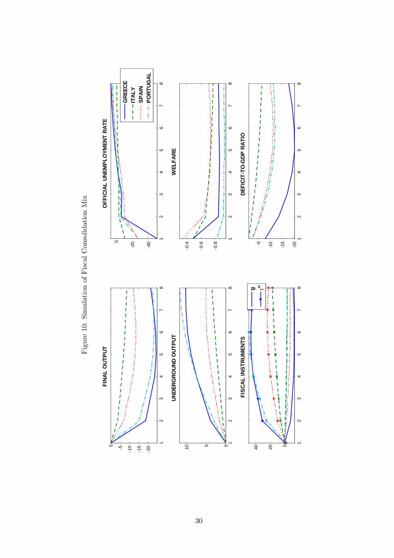
Figure10:SimulationofFiscalConsolidationMix

12

34

56

78

­20

­15

­10­50

FINA

L O

UTPU

T

12

34

56

78

­40

­200

OFF

ICIA

L UN

EMPL

OYM

ENT 

RATE

12

34

56

78

0510

UNDE

RGRO

UND 

OUT

PUT

12

34

56

78

­0.8

­0.6

­0.4

WEL

FARE

12

34

56

78

02040

FISC

AL IN

STRU

MEN

TS

12

34

56

78

­20

­15

­10­5

DEFI

CIT­

TO­G

DP R

ATIO

g τn

GRE

ECE

ITAL

YSP

AIN

PORT

UGAL

30

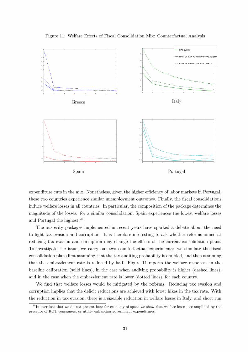
Figure 11: Welfare E¤ects of Fiscal Consolidation Mix: Counterfactual Analysis

1 2 3 4 5 6 7 8

­0. 8

­0. 6

­0. 4

­0. 2

0

0. 2

0. 4

0. 6

0. 8

1

1. 2

Greece

1 2 3 4 5 6 7 8

­0. 7

­0. 6

­0. 5

­0. 4

­0. 3

­0. 2

  B ASEL IN E

  H IG H ER  T AX AU D IT IN G  PR O B AB IL IT Y

  L O W ER  EM B EZ Z L EM EN T  R AT E

Italy

1 2 3 4 5 6 7 8

­0.5

0

0.5

1

1.5

2

2.5

Spain

1 2 3 4 5 6 7 8

­0. 92

­0. 9

­0. 88

­0. 86

­0. 84

­0. 82

­0. 8

Portugal

expenditure cuts in the mix. Nonetheless, given the higher e¢ ciency of labor markets in Portugal,

these two countries experience similar unemployment outcomes. Finally, the �scal consolidations

induce welfare losses in all countries. In particular, the composition of the package determines the

magnitude of the losses: for a similar consolidation, Spain experiences the lowest welfare losses

and Portugal the highest.20

The austerity packages implemented in recent years have sparked a debate about the need

to �ght tax evasion and corruption. It is therefore interesting to ask whether reforms aimed at

reducing tax evasion and corruption may change the e¤ects of the current consolidation plans.

To investigate the issue, we carry out two counterfactual experiments: we simulate the �scal

consolidation plans �rst assuming that the tax auditing probability is doubled, and then assuming

that the embezzlement rate is reduced by half. Figure 11 reports the welfare responses in the

baseline calibration (solid lines), in the case when auditing probability is higher (dashed lines),

and in the case when the embezzlement rate is lower (dotted lines), for each country.

We �nd that welfare losses would be mitigated by the reforms. Reducing tax evasion and

corruption implies that the de�cit reductions are achieved with lower hikes in the tax rate. With

the reduction in tax evasion, there is a sizeable reduction in welfare losses in Italy, and short run

20 In exercises that we do not present here for economy of space we show that welfare losses are ampli�ed by thepresence of ROT consumers, or utility enhancing government expenditures.

31

welfare gains for Greece and Spain, which have relatively more expenditure-based consolidation

policies. When corruption is reduced, welfare improves substantially in Italy, and in Greece on

impact, since these two countries have a higher degree of corruption. In Spain, where the level of

corruption is lower, the gains from reducing corruption are small relative to �ghting tax evasion.

Note that the welfare gains in Portugal are small, since the heavy reliance on tax hikes continues

to imply large welfare losses in both the counterfactual cases.

5 Conclusions

Empirical evidence indicates that accounting for tax evasion and corruption is key for under-

standing the e¤ects of �scal consolidation. A New Keynesian DSGE model with involuntary

unemployment, an informal sector and public corruption, demonstrates that these two features

amplify the contractionary e¤ects of labor tax hikes, while they mitigate the e¤ects of expenditure

cuts. It also shows that the instrument used to achieve �scal consolidation a¤ects the incentives

of agents to produce in the informal sector. Consistent with VAR evidence obtained for Italian,

spending cuts reduce the size of the informal economy, while tax hikes increase it.

Given the model�s ability to reproduce the qualitative features of the data, we analyze how

current �scal consolidation plans in Greece, Italy, Portugal and Spain a¤ect tax evasion, output,

unemployment and welfare. The model predicts increasing levels of tax evasion during the con-

solidation in all countries, and prolonged output and welfare losses. Greece su¤ers heavy losses

due to the severity of the austerity package implemented; Portugal experiences the largest drops

in welfare because of the heavy use of tax hikes in their consolidation package. Furthermore,

the welfare costs of these consolidations would have been smaller if tax evasion and corruption

had been reduced. Hence, reforms aimed at �ghting public corruption and tax evasion should go

hand-in-hand with austerity measures in order to mitigate the welfare costs of �scal consolidations.

Our exercise is the �rst attempt to analyze the e¤ects of �scal consolidation in the presence

of tax evasion and corruption. Since the model is stylized, it leaves out important aspects of

reality that could a¤ect our conclusions. For example, in our economy there is a representative

household, and so we cannot assess the e¤ects of tax evasion and corruption on income inequality.

Also, we consider only cuts in government consumption expenditures and not in other items of

the government budget. Furthermore, our model does not allow for evasion of consumption taxes,

which is an important component of tax evasion in Southern European countries. Finally, the

model treats the degree of public corruption as a parameter, which does not allow it to respond

to cyclical factors or to interact with tax evasion. We leave these extensions for future research.

32

References

[1] Alesina A., C. Favero and F. Giavazzi, 2013, �The Output E¤ect of Fiscal Consolidations�,

Working Papers 478, IGIER, Bocconi University.

[2] Ardizzi G., C. Petraglia, M. Piacenza and G. Tutati, 2012, �Measuring the Underground

Economy with the Currency Demand Approach: A Reinterpretation of the Methodology,

with an Application to Italy�, Bank of Italy Working Paper Series, No. 864.

[3] Auerbach, A., and Y. Gorodnichenko, 2012, �Fiscal Multipliers in Recession and Expansion�,

NBER Chapters, Fiscal Policy After the Financial Crisis, 63-98.

[4] Bermperoglou D., E. Pappa and E. Vella, 2014, �Spending Cuts and Their E¤ects on Output,

Unemployment and the De�cit�, Unpublished Manuscript.

[5] Blanchard, O. and D. Leigh, 2013, �Growth Forecast Errors and Fiscal Multipliers�, IMF

Working Papers 13/1.

[6] Boeri T. and P. Garibaldi, 2007, �Shadow Sorting,�NBER International Seminar on Macro-

economics 2005, MIT Press, 125-163.

[7] Brückner, M. and E. Pappa, 2012, �Fiscal Expansions, Unemployment, and Labor Force

Participation: Theory and Evidence�, International Economic Review, 53(4), 1205-1228.

[8] Buehn A. and F. Schneider, 2012, �Corruption and the Shadow Economy: Like Oil and

Vinegar, Like Water and Fire?�, International Tax and Public Finance, 19(1), 172-194.

[9] Busato F. and B. Chiarini, 2004, �Market and Underground Activities in a Two-Sector Dy-

namic Equilibrium Model�, Economic Theory, 23(4), 831-861.

[10] Calvo, G. A., 1983, �Staggered Prices in a Utility-Maximizing Framework,�Journal of Mon-

etary Economics, 12(3), 383-398.

[11] Campolmi A. and S. Gnocchi, 2014, �Labor Market Participation, Unemployment and Mon-

etary Policy�, Bank of Canada Working Paper No. 2014/9.

[12] Charron N., V. Lapuente and L. Dijkstra, 2012, �Regional Governance Matters: A Study

on the Regional Variation in Quality of Government within the EU�, European Commission

Working Paper Series No. 01/2012.

[13] Devries, P., J. Guajardo, D. Leigh and A. Pescatori, 2011, �A New Action-based Dataset of

Fiscal Consolidation�, IMF Working Papers 11/128

[14] Eggertsson, G. B., and P. Krugman, 2012. �Debt, Deleveraging, and the Liquidity Trap: A

Fisher-Minsky-Koo Approach�The Quarterly Journal of Economics, 127(3), 1469-1513.

[15] Elgin C. and O. Öztunah O., 2012, �Shadow Economies Around the World: Model Based

Estimates�, working paper.

33

[16] Erceg, C. and J. Lindé, 2013, �Fiscal Consolidation in a Currency Union: Spending Cuts vs.

Tax Hikes,�Journal of Economic Dynamics and Control, 37(2), 422-445.

[17] Fugazza M. and J.-F. Jacques, 2004, �Labor Market Institutions, Taxation and the Under-

ground Economy,�Journal of Public Economics, 88, 395-418.

[18] Galí, J., J. D. López-Salido and J. Vallés, 2007, �Understanding the E¤ects of Government

Spending on Consumption,�Journal of the European Economic Association, 5(1), 227-270.

[19] Gestha, 2014, �La Economía Sumergida Pasa Factura. El Avance del Fraude en España

Durante la Crisis�, Madrid, enero de 2014.

[20] Hansen G., 1985, �Indivisible Labor and the Business Cycle,�Journal of Monetary Economics,

16, 309-27.

[21] Hansen L. P., and K. Singleton, 1983, �Stochastic Consumption, Risk Aversion and the

Temporal Behavior of Asset Returns�, Journal of Political Economy, 91, 249-265.

[22] ISTAT, 2010, �La Misura dell�Economia Sommersa Secondo le Statistiche U¢ cialli. Anni

2000-2008,�Conti-Nazionali-Statistiche in Breve, Istituto Nazionale di Statistica, Rome.

[23] Martin J., 1996, �Measures of Replacement Rates for the Purpose of International Compari-

son: A Note�, OECD Economic Studies, 26(1), 98-118.

[24] Martin, P. and T. Philippon, 2014, �Inspecting the Mechanism: Leverage and the Great

Recession in the Eurozone,�Unpublished Manuscript.

[25] OECD, 2012, Restoring Public Finances, 2012 Update, OECD Publishing.

http://dx.doi.org/10.1787/9789264179455-en

[26] Orsi R., D. Raggi and F. Turino, 2014, �Size, Trend, and Policy Implications of the Under-

ground Economy�, forthcoming in the Review of Economic Dynamics.

[27] Peracchi F. and E. Viviano, 2004, �An Empirical Micro Matching Model with an Application

to Italy and Spain�, Temi di discussione No. 538, Banca d Italia.

[28] Perotti, R., 1996, �Fiscal Consolidation in the Europe: Composition Matters�, American

Economic Review Papers and Proceedings, 86(2), 105-110.

[29] Perotti, R., 2005, �Estimating the E¤ects of Fiscal Policy in OECD Countries�, Proceedings,

Federal Reserve Bank of San Francisco.

[30] Ravn, M. O., 2008, �The Consumption-Tightness Puzzle�, NBER Chapters, NBER Interna-

tional Seminar on Macroeconomics 2006, 9-63.

[31] Restrepo-Echavarria P., 2014, �Macroeconomic Volatility: The Role of the Informal Economy,�

European Economic Review, 70, 454-469.

34

[32] Schneider F. and A. Buehn, 2012, �Shadow Economies in Highly Developed OECD Countries:

What are the Driving Forces?�, IZA discussion paper No. 6891, Institute for the study of labor,

University of Bonn, Bonn, 2012.

35