Fitting log-linear models in sparse contingency tables usingthe eMLEloglin R package

Matthew Friedlander

Abstract

Log-linear modeling is a popular method for the analysis of contingency table data. Whenthe table is sparse, and the data falls on a proper face F of the convex support, there areconsequences on model inference and model selection. Knowledge of the cells determiningF is crucial to mitigating these effects. We introduce the R package (R Core Team (2016))eMLEloglin for determining F and passing that information on to the glm() function to fit themodel properly.

1 Introduction

Data in the form of a contingency table arise when individuals are cross classified according toa finite number of criteria. Log-linear modeling (see e.g., Agresti (1990), Christensen (1997), orBishop et al. (1975)) is a popular and effective methodology for analyzing such data enabling thepractitioner to make inferences about dependencies between the various criteria. For hierarchicallog-linear models, the interactions between the criteria can be represented in the form of a graph; thevertices represent the criteria and the presence or absence of an edge between two criteria indicateswhether or not the two are conditionally independent (Lauritzen (1996)). This kind of graphicalsummary greatly facilitates the interpretation of a given model.

Log-linear models are typically fit by maximum likelihood estimation (i.e. we attempt computethe MLE of the expected cell counts and log-linear parameters). It has been known for many yearsthat problems arise when the sufficient statistic falls on the boundary of the convex support, sayC, of the model (Feinberg and Rinaldo (2007)). This generally occurs in sparse contingency withmany zero cells. In such cases, algorithms for computing the MLE can fail to converge. Moreover,the effective model dimension will be reduced and the degrees of freedom of the usual goodness offit statistics will be incorrect. Only fairly recently, have algorithms been developed to begin to dealwith this situation (see Eriksson et al. (2006), Geyer (2009) and Feinberg and Rinaldo (2012)). Itturns out that identification of the face F of C containing the data in its relative interior is crucialto efficient and reliable computation of the MLE and of the effective model dimension. If F = Cthen the MLE exists and it’s calculation is straightforward. If not (i.e. F ⊂ C), the log-likelihoodhas its maximum on the boundary and remedial steps must be taken to find and compute thoseparameters that can be estimated.

The outline of this paper is as follows. In Section 2, we describe necessary and sufficient condi-tions for the existence of the MLE. In Section 3, we place these conditions in the context of convexgeometry. In Section 4, we describe a linear programming algorithm to find F . We then discusshow to compute ML estimates and find the effective model dimension. In Section 5, we introducethe eMLEloglin R package for carrying out the tasks described in Section 4.

1

2 Conditions for the existence of the MLE

Let V be a finite set of indices representing |V | criteria. We assume that the criterion labeled byv ∈ V can take values in a finite set Iv. The resulting counts are gathered in a contingency tablesuch that

I =∏v∈V

Iv

is the set of cells i = (v ∈ V ). The vector of cell counts is denoted n = (n(i), i ∈ I) with corre-sponding mean m(i) = E(n) = (m(i), i ∈ I). For D ⊂ V,

ID =∏v∈D

Iv

is the set of cells iD = (iv, v ∈ D) in the D-marginal table. The marginal counts are n(iD) =∑j:jD=iD

n(j) with m(iD) = E (n(iD)).We assume that the components of n are independent and follow a Poisson distribution (i.e.

Poisson sampling) and that the cell means are modeled according to a hierarchical model

log (m) = Xθ

where X is an |I|×p design matrix with rows {fi, i ∈ I} and θ is a p-vector of log-linear parameterswith θ ∈ Rp. The results herein also apply under multinomial or product multinomial sampling.We assume that the first component of fi is 1 for all i ∈ I and that “baseline constraints” are usedmaking the f ′is binary 0/1 vectors. For each cell, i ∈ I, we have logm(i) = 〈fi, θ〉.

The sufficient statistic t = XTn has the probability distribution in the natural exponential famil

f(t) = exp

(〈θ, t〉 −

∑i∈I

exp (〈fi, θ〉)

)ν (dt)

with respect to a discrete measure ν that has convex support

Cp =

{∑i∈I

y(i)fi, y(i) ≥ 0, i ∈ I

}= cone {xi, i ∈ I}

i.e. the convex cone generated by the rows of the design matrix X. The log-likelihood, as a functionof m, is

l(m) =∑i∈I

n(i) logm(i)−∑i∈I

m(i)

Let M be the column space of X. It is well known that the log-likelihood is strictly concave witha unique maximizer m̂ = argsuplogm∈Ml(m) that satisfies XT m̂ = t.

Definition 2.1. If m̂ > 0, we say that m̂ is the MLE of m while if m̂(i) = 0 for some i ∈ I we callm̂ the extended MLE.

The following important theorem from Haberman (1974) gives necessary and sufficient conditionsfor m̂ > 0, i.e. the existence of the MLE.

Theorem 2.2. The MLE exists if and only if there exists a y such that XTy = 0 and y + n > 0.

2

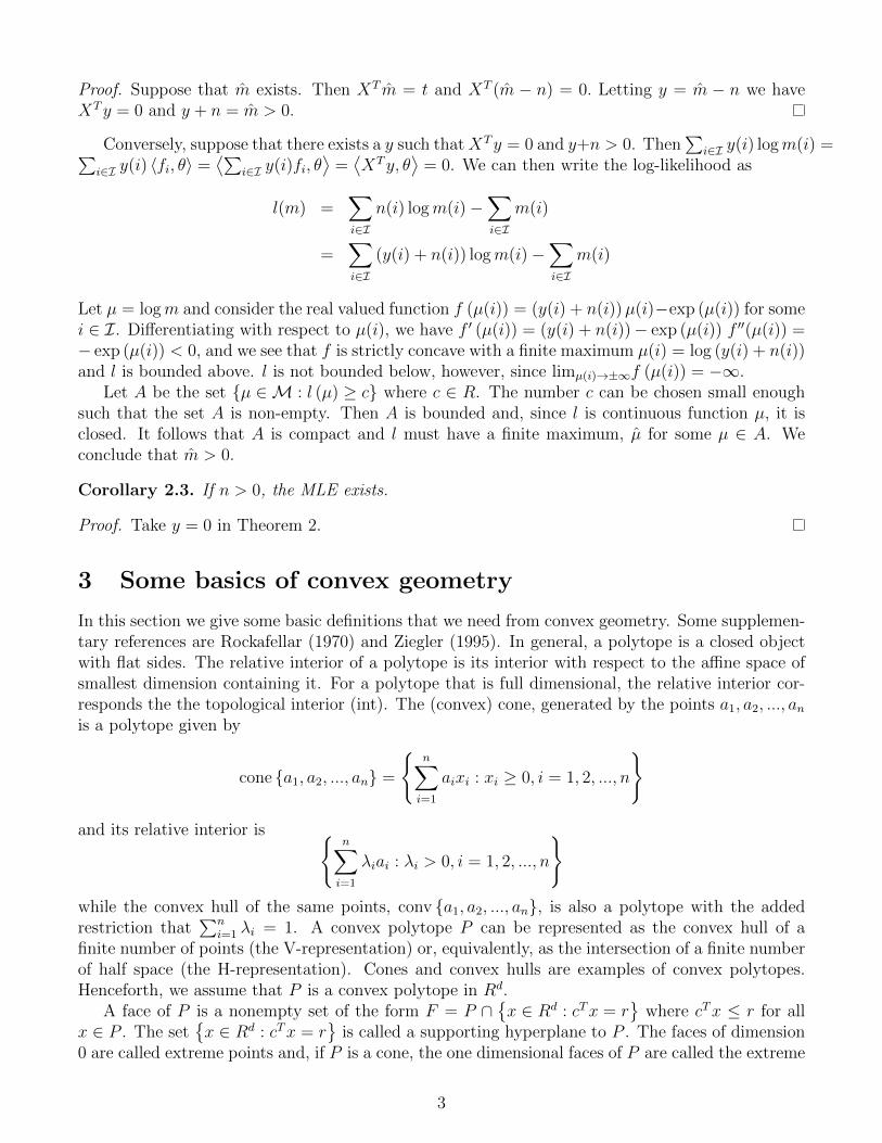
Proof. Suppose that m̂ exists. Then XT m̂ = t and XT (m̂ − n) = 0. Letting y = m̂ − n we haveXTy = 0 and y + n = m̂ > 0.

Conversely, suppose that there exists a y such thatXTy = 0 and y+n > 0. Then∑

i∈I y(i) logm(i) =∑i∈I y(i) 〈fi, θ〉 =

⟨∑i∈I y(i)fi, θ

⟩=⟨XTy, θ

⟩= 0. We can then write the log-likelihood as

l(m) =∑i∈I

n(i) logm(i)−∑i∈I

m(i)

=∑i∈I

(y(i) + n(i)) logm(i)−∑i∈I

m(i)

Let µ = logm and consider the real valued function f (µ(i)) = (y(i) + n(i))µ(i)−exp (µ(i)) for somei ∈ I. Differentiating with respect to µ(i), we have f ′ (µ(i)) = (y(i) + n(i))− exp (µ(i)) f ′′(µ(i)) =− exp (µ(i)) < 0, and we see that f is strictly concave with a finite maximum µ(i) = log (y(i) + n(i))and l is bounded above. l is not bounded below, however, since limµ(i)→±∞f (µ(i)) = −∞.

Let A be the set {µ ∈M : l (µ) ≥ c} where c ∈ R. The number c can be chosen small enoughsuch that the set A is non-empty. Then A is bounded and, since l is continuous function µ, it isclosed. It follows that A is compact and l must have a finite maximum, µ̂ for some µ ∈ A. Weconclude that m̂ > 0.

Corollary 2.3. If n > 0, the MLE exists.

Proof. Take y = 0 in Theorem 2.

3 Some basics of convex geometry

In this section we give some basic definitions that we need from convex geometry. Some supplemen-tary references are Rockafellar (1970) and Ziegler (1995). In general, a polytope is a closed objectwith flat sides. The relative interior of a polytope is its interior with respect to the affine space ofsmallest dimension containing it. For a polytope that is full dimensional, the relative interior cor-responds the the topological interior (int). The (convex) cone, generated by the points a1, a2, ..., anis a polytope given by

cone {a1, a2, ..., an} =

{n∑i=1

aixi : xi ≥ 0, i = 1, 2, ..., n

}

and its relative interior is {n∑i=1

λiai : λi > 0, i = 1, 2, ..., n

}while the convex hull of the same points, conv {a1, a2, ..., an}, is also a polytope with the addedrestriction that

∑ni=1 λi = 1. A convex polytope P can be represented as the convex hull of a

finite number of points (the V-representation) or, equivalently, as the intersection of a finite numberof half space (the H-representation). Cones and convex hulls are examples of convex polytopes.Henceforth, we assume that P is a convex polytope in Rd.

A face of P is a nonempty set of the form F = P ∩{x ∈ Rd : cTx = r

}where cTx ≤ r for all

x ∈ P . The set{x ∈ Rd : cTx = r

}is called a supporting hyperplane to P . The faces of dimension

0 are called extreme points and, if P is a cone, the one dimensional faces of P are called the extreme

3

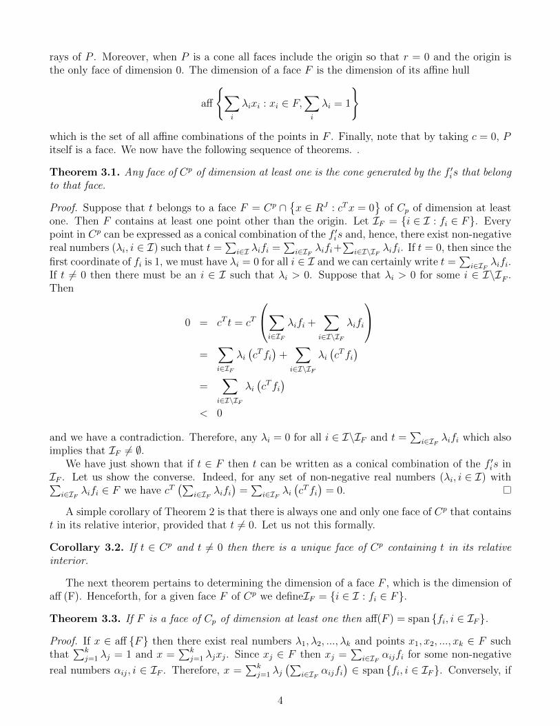
rays of P . Moreover, when P is a cone all faces include the origin so that r = 0 and the origin isthe only face of dimension 0. The dimension of a face F is the dimension of its affine hull

aff

{∑i

λixi : xi ∈ F,∑i

λi = 1

}

which is the set of all affine combinations of the points in F . Finally, note that by taking c = 0, Pitself is a face. We now have the following sequence of theorems. .

Theorem 3.1. Any face of Cp of dimension at least one is the cone generated by the f ′is that belongto that face.

Proof. Suppose that t belongs to a face F = Cp ∩{x ∈ RJ : cTx = 0

}of Cp of dimension at least

one. Then F contains at least one point other than the origin. Let IF = {i ∈ I : fi ∈ F}. Everypoint in Cp can be expressed as a conical combination of the f ′is and, hence, there exist non-negativereal numbers (λi, i ∈ I) such that t =

∑i∈I λifi =

∑i∈IF λifi+

∑i∈I\IF λifi. If t = 0, then since the

first coordinate of fi is 1, we must have λi = 0 for all i ∈ I and we can certainly write t =∑

i∈IF λifi.If t 6= 0 then there must be an i ∈ I such that λi > 0. Suppose that λi > 0 for some i ∈ I\IF .Then

0 = cT t = cT

∑i∈IF

λifi +∑

i∈I\IF

λifi

=

∑i∈IF

λi(cTfi

)+∑

i∈I\IF

λi(cTfi

)=

∑i∈I\IF

λi(cTfi

)< 0

and we have a contradiction. Therefore, any λi = 0 for all i ∈ I\IF and t =∑

i∈IF λifi which alsoimplies that IF 6= ∅.

We have just shown that if t ∈ F then t can be written as a conical combination of the f ′is inIF . Let us show the converse. Indeed, for any set of non-negative real numbers (λi, i ∈ I) with∑

i∈IF λifi ∈ F we have cT(∑

i∈IF λifi)

=∑

i∈IF λi(cTfi

)= 0.

A simple corollary of Theorem 2 is that there is always one and only one face of Cp that containst in its relative interior, provided that t 6= 0. Let us not this formally.

Corollary 3.2. If t ∈ Cp and t 6= 0 then there is a unique face of Cp containing t in its relativeinterior.

The next theorem pertains to determining the dimension of a face F , which is the dimension ofaff (F). Henceforth, for a given face F of Cp we defineIF = {i ∈ I : fi ∈ F}.

Theorem 3.3. If F is a face of Cp of dimension at least one then aff(F ) = span {fi, i ∈ IF}.

Proof. If x ∈ aff {F} then there exist real numbers λ1, λ2, ..., λk and points x1, x2, ..., xk ∈ F suchthat

∑kj=1 λj = 1 and x =

∑kj=1 λjxj. Since xj ∈ F then xj =

∑i∈IF αijfi for some non-negative

real numbers αij, i ∈ IF . Therefore, x =∑k

j=1 λj(∑

i∈IF αijfi)∈ span {fi, i ∈ IF}. Conversely, if

4

x ∈ span {fi, i ∈ IF} then x =∑

i∈IF λifi for some real numbers λi, i ∈ IF . Since 0 ∈ F we canwrite

x =

(1−

∑i∈IF

λi

)0 +

∑i∈IF

λifi

which is an affine combination of points in F . Therefore, x ∈ aff(F ).Since there are p linearly independent f ′is, it follows that the dimension of Cp is p.

Theorem 3.4. If F is a face of Cp of dimension at least one then the extreme rays of F are thef ′is that belong to that face.

Proof. Suppose that x ∈ F which implies that x =∑

i∈IF λifi for some non-negative real numbersλi, i ∈ IF with at least one λi > 0. If x is an extreme ray then we must have exactly one λi > 0.For if not, then x would be a conical combination of two linearly independent vectors (none of thef ′is are scalar multiples of one another). But then x = λifi.

For a given, fj ∈ F we need to show that fj is an extreme ray. Suppose that this is not thecase. Then fj can be written as a conic combination of two vectors x1, x2 ∈ Cp where x1 6= kx2forsome k > 0. That is, fj = λ1x1 + λ2x2 for some λ1λ2 > 0. But, by Theorem 2, x1 =

∑i∈IF αi1fi

and x2 =∑

i∈IF αi2fi so that

fj = λ1∑i∈IF

αi1fi + λ2∑i∈IF

αi2fi

Recalling that all the f ′is are distinct binary 0/1 vectors we must have a contradiction since IF ⊇{fj}.

The following corollary of Theorem 2 is due to Feinberg and Rinaldo (2012).

Corollary 3.5. The MLE exists if and only if t ∈ ri (Cp).

Proof. Suppose that the MLE exists. Then by Theorem 2, there exists a y such that XTy = 0 andy+n > 0. But then t = XT (y + n) where y+n > 0 and hence t ∈ ri (Cp). Now suppose t ∈ ri (Cp).By definition, there exists an y > 0 such that XTy = t = XTn. But then XT (y − n) = 0 andn+ (y − n) > 0 and the MLE exists (by Theorem 2).

4 An algorithm to determine IFWe have seen in Section 3, in particular, corollary (5), that there is a unique face F of Cp containingthe sufficient statistic t = XTn in its relative interior. We turn now to finding F ; for the MLEexists if and only if F = Cp. With IF = {i ∈ I : fi ∈ F} we let XF be an IF × J matrix with rowsfi, i ∈ IF . By Theorem 4, we know that F = cone {fi, i ∈ IF} and by Theorem 6, the dimensionof F is pF = rank (XF ). Equipped with the following theorem, we can take an approach similarto Geyer (2009) and Feinberg and Rinaldo (2012), and finds IF by solving a sequence of linearprograms.

Theorem 4.1. Any a ≥ 0 in RI such that t = XTa must have a(i) = 0 for any i ∈ I\IF .

5

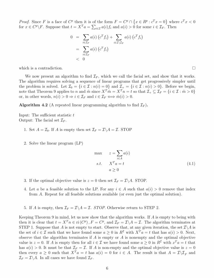
Proof. Since F is a face of Cp then it is of the form F = Cp ∩{x ∈ Rp : cTx = 0

}where cTx < 0

for x ∈ Cp\F . Suppose that t = XTa =∑

i∈I a(i)fi and a(i) > 0 for some i ∈ IF . Then

0 =∑i∈IF

a(i)(cTfi

)+∑

i∈I\IF

a(i)(cTfi

)=

∑i∈IF

a(i)(cTfi

)< 0

which is a contradiction.

We now present an algorithm to find IF , which we call the facial set, and show that it works.The algorithm requires solving a sequence of linear programs that get progressively simpler untilthe problem is solved. Let I0 = {i ∈ I : n(i) = 0} and I+ = {i ∈ I : n(i) > 0}. Before we begin,note that Theorem 9 applies to n and m̂ since XT m̂ = XTn = t so that I+ ⊆ IF = {i ∈ I : m̂ > 0}or, in other words, n(i) > 0⇒ i ∈ IF and i ∈ IF ⇐⇒ m̂(i) > 0.

Algorithm 4.2 (A repeated linear programming algorithm to find IF )..

Input: The sufficient statistic tOutput: The facial set IF .

1. Set A = I0. If A is empty then set IF = I\A = I. STOP

2. Solve the linear program (LP)

max z =∑i∈A

a(i)

s.t. XTa = t (4.1)

a ≥ 0

3. If the optimal objective value is z = 0 then set IF = I\A. STOP.

4. Let a be a feasible solution to the LP. For any i ∈ A such that a(i) > 0 remove that indexfrom A. Repeat for all feasbile solutions available (or even just the optimal solution).

5. If A is empty, then IF = I\A = I. STOP. Otherwise return to STEP 2.

Keeping Theorem 9 in mind, let us now show that the algorithm works. If A is empty to being withthen it is clear that t = XTn ∈ ri (Cp) , F = Cp, and IF = I\A = I. The algorithm terminates atSTEP 1. Suppose that A is not empty to start. Observe that, at any given iteration, the set I\A isthe set of i ∈ I such that we have found some a ≥ 0 in RI with XTa = t that has a(i) > 0. Next,observe that the algorithm terminates if A is empty or A is nonempty and the optimal objectivevalue is z = 0. If A is empty then for all i ∈ I we have found some a ≥ 0 in RI with xTa = t thathas a(i) > 0. It must be that IF = I. If A is non-empty and the optimal objective value is z = 0then every a ≥ 0 such that XTa = t has a(i) = 0 for i ∈ A. The result is that A = I\IF andIF = I\A. In all cases we have found IF .

6

Now, suppose that y ∈ RI such that y(i) > 0 ⇐⇒ n(i) > 0. Then t′ = XTy =∑

i∈I y(i)fi andt = XTn =

∑i∈I n(i)fi belong to the same face F . Therefore, it is the location of the zero cells

in n that determines F as opposed to the magnitude of the nonzero entries. For this reason, it issimplest to let s

y(i) =

{1 n(i) > 0

0 n(i) = 0

and find IF using t′.For models where m is Markov with respect to a decomposable graph G the MLE (or extended

MLE) a closed form expression for its computation exists. Theoretically, for such models, one neednot resort to linear programming to find IF , since m̂ can be computed exactly. Once this is donewe know that IF = {i ∈ I : m̂(i) > 0}. Practically speaking though, it is simpler to use algorithm10 for any model without first determining decomposability.

We now give an example applying Algorithm 10.

Example 4.3. Consider a 3× 3× 3 table for variables a, b, c with counts:

0 1 00 1 11 1 1

1 1 11 1 11 0 0

1 1 11 1 11 0 0

and the model [ab][bc][ac]. Suppose Ia = Ib = Ic = {1, 2, 3}. The leftmost array correspondsto c = 1, the middle to c = 2, and the rightmost to c = 3. Let us apply our the algorithm to findF for this data set. We begin, at STEP 1, by setting

A = I0 = {111, 131, 211, 322, 332, 323}

where, by an abuse of notation, 131, refers to cell i = (1, 3, 1) with a = 1, b = 3, c = 1. Since A isnonempty we proceed to STEP 2. The optimal solution to the (1) has a(131) > 0 and so we removethe cell 131 from A to get

A = {111, 211, 322, 332, 323, 333}

and return to STEP 2. Resolving (1) we find that, this time, the optimal objective value is 0. Atthis point we set IF = I\A = I+ ∪ {131} and the algorithm terminates. The dimension of F isrank (XF ), which in this case, is 18.

In the remainder of this section, we proceed to show that when F ⊂ C, maximum likelihoodestimation can proceed almost as usual conditional on t ∈ F . Recall once more, the likelihood as afunction of m.

L(m) =∏i∈I

exp (−m(i))m(i)n(i)

=∏i∈IF

exp (−m(i))m(i)n(i)∏

i∈I\IF

exp (−m(i))m(i)n(i)

7

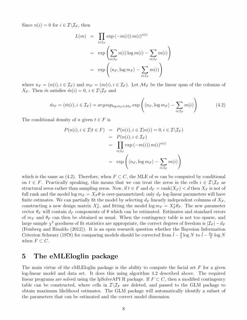
Since n(i) = 0 for i ∈ I\IF , then

L(m) =∏i∈IF

exp (−m(i))m(i)n(i)

= exp

(∑i∈IF

n(i) logm(i)−∑i∈IF

m(i)

)

= exp

(〈nF , logmF 〉 −

∑i∈IF

m(i)

)

where nF = (n(i), i ∈ IF ) and mF = (m(i), i ∈ IF ). Let MF be the linear span of the columns ofXF . Then m̂ satisfies m̂(i) = 0, i ∈ I\IF and

m̂F = (m̂(i), i ∈ IF ) = argsuplogmF∈MFexp

(〈nF , logmF 〉 −

∑i∈IF

m(i)

)(4.2)

The conditional density of n given t ∈ F is

P (n(i), i ∈ I|t ∈ F ) = P (n(i), i ∈ I|n(i) = 0, i ∈ I\IF )

= P (n(i), i ∈ IF )

=∏i∈IF

exp (−m(i))m(i)n(i)

= exp

(〈nF , logmF 〉 −

∑i∈IF

m(i)

)

which is the same as (4.2). Therefore, when F ⊂ C, the MLE of m can be computed by conditionalon t ∈ F . Practically speaking, this means that we can treat the zeros in the cells i ∈ I\IF asstructural zeros rather than sampling zeros. Now, if t ∈ F and dF = rank(XF ) < d then XF is not offull rank and the model logmF = XF θ is over-parametrized; only dF log-linear parameters will havefinite estimates. We can partially fit the model by selecting dF linearly independent columns of XF ,constructing a new design matrix X∗F , and fitting the model logmF = X∗F θF . The new parametervector θF will contain dF components of θ which can be estimated. Estimates and standard errorsof mF and θF can then be obtained as usual. When the contingency table is not too sparse, andlarge sample χ2 goodness of fit statistics are appropriate, the correct degrees of freedom is |IF |−dF(Feinberg and Rinaldo (2012)). It is an open research question whether the Bayesian InformationCriterion Schwarz (1978) for comparing models should be corrected from l̂− d

2logN to l̂− dF

2logN

when F ⊂ C.

5 The eMLEloglin package

The main virtue of the eMLEloglin package is the ability to compute the facial set F for a givenlog-linear model and data set. It does this using algorithm 4.2 described above. The requiredlinear programs are solved using the lpSolveAPI R package. If F ⊂ C, then a modified contingencytable can be constructed, where cells in I\IF are deleted, and passed to the GLM package toobtain maximum likelihood estimates. The GLM package will automatically identify a subset ofthe parameters that can be estimated and the correct model dimension.

8

The eMLEloglin package includes a sparse dataset from the household study at Rochdale re-ferred to in Whittaker (1990). The Rochdale data set is a contingency table representing the crossclassification of 665 individuals according to 8 binary variables. The study was conducted to elicitinformation about factors affecting the pattern of economic life in Rochdale, England. The vari-ables are as follows: a. wife economically active (no, yes); b. age of wife >38 (no, yes); c. husbandunemployed (no, yes); d. child≤ 4 (no, yes); e. wife’s education, highschool+ (no, yes); f. husband’seducation, highschool+ (no, yes); g. Asian origin (no, yes); h. other household member working(no, yes). The table is sparse have 165 counts of zero, 217 counts with at most three observations,but also a few large counts with 30 or more observations.

Example 5.1. Consider the following 2× 2× 2 contingency table for variables a, b, c with counts:

0 11 1

1 11 0

and the model [ab][bc][ac]. Suppose Ia = Ib = Ic = {1, 2}. The leftmost array corresponds toc = 1, and the rightmost array to c = 2. This is one of the earliest known examples identified wherethe MLE does not exist Haberman (1974). We now show how to compute F using the eMLEloglinpackage. We first create a contingency table to hold the data:

> x <- matrix(nrow = 8, ncol = 4)

> x[,1] <- c(0,0,0,0,1,1,1,1)

> x[,2] <- c(0,0,1,1,0,0,1,1)

> x[,3] <- c(0,1,0,1,0,1,0,1)

> x[,4] <- c(0,1,2,1,4,1,3,0)

> colnames(x) = c("a", "b", "c", "freq")

> x <- as.data.frame(x, row.names = rep(,8))

>

> x a b c freq

1 0 0 0 0

2 0 0 1 1

3 0 1 0 2

4 0 1 1 1

5 1 0 0 4

6 1 0 1 1

7 1 1 0 3

8 1 1 1 0

We can then use the facial set function:

> f <- facial_set (data = x, formula = freq ~ a*b + a*c + b*c)

> f

$formula

freq ~ a*b + a*c + b*c

$model.dimension

[1] 7

$status

9

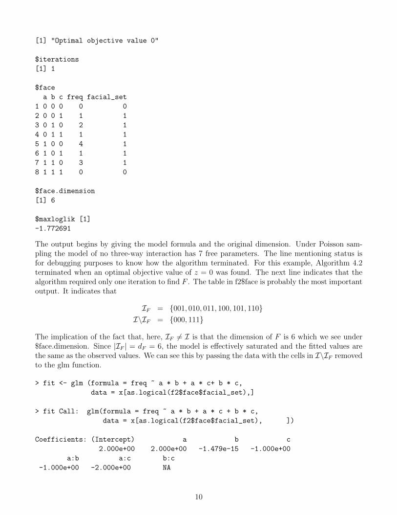
[1] "Optimal objective value 0"

$iterations

[1] 1

$face

a b c freq facial_set

1 0 0 0 0 0

2 0 0 1 1 1

3 0 1 0 2 1

4 0 1 1 1 1

5 1 0 0 4 1

6 1 0 1 1 1

7 1 1 0 3 1

8 1 1 1 0 0

$face.dimension

[1] 6

$maxloglik [1]

-1.772691

The output begins by giving the model formula and the original dimension. Under Poisson sam-pling the model of no three-way interaction has 7 free parameters. The line mentioning status isfor debugging purposes to know how the algorithm terminated. For this example, Algorithm 4.2terminated when an optimal objective value of z = 0 was found. The next line indicates that thealgorithm required only one iteration to find F . The table in f2$face is probably the most importantoutput. It indicates that

IF = {001, 010, 011, 100, 101, 110}I\IF = {000, 111}

The implication of the fact that, here, IF 6= I is that the dimension of F is 6 which we see under$face.dimension. Since |IF | = dF = 6, the model is effectively saturated and the fitted values arethe same as the observed values. We can see this by passing the data with the cells in I\IF removedto the glm function.

> fit <- glm (formula = freq ~ a * b + a * c+ b * c,

data = x[as.logical(f2$face$facial_set),]

> fit Call: glm(formula = freq ~ a * b + a * c + b * c,

data = x[as.logical(f2$face$facial_set), ])

Coefficients: (Intercept) a b c

2.000e+00 2.000e+00 -1.479e-15 -1.000e+00

a:b a:c b:c

-1.000e+00 -2.000e+00 NA

10

Degrees of Freedom: 5 Total (i.e. Null); 0 Residual

Null Deviance: 8 Residual Deviance: 6.015e-30

AIC: -383.4

> fit$fitted.values

2 3 4 5 6 7

1 2 1 4 1 3

As expected, one parameter is not able to be estimated; and R handles this automatically. Notethat the residual degrees of freedom is correctly calculated to be |IF | = dF = 0. Let us workthrough a larger example now with the Rochdale data.

Example 5.2. The Rochdale data comes preloaded with the package. Suppose we are interestedin the model |ad|ae|be|ce|ed|acg|dg|fg|bdh| which is the model with the highest corrected BIC forthis data set. We give a list of the top models by corrected and uncorrected BIC below for this dataset. The required R code to find the facial set for this model is:

data(rochdale)

f <- facial_set (data = rochdale,

formula = freq ~ a*d + a*e + b*e + c*e + e*f +

a*c*g + d*g + f*g + b*d*h)

From the output we see that the model lies on a face of dimension 22. Since the original modeldimension is 24, two parameters will not be estimable. Given the sparsity of the table, a goodnessof fit test would not be appropriate. The fitted model can be obtained from the GLM function withthe code:

fit <- glm (formula = freq ~ a*d + a*e + b*e + c*e + e*f +

a*c*g + d*g + f*g + b*d*h)

data = rochdale[as.logical(f2$face$facial_set),])

The GLM function automatically determines that θacg and θbdh can not be estimated; which isbecause the acg and bdh margins are both zero. The residual degrees of freedom is correctlycalculated at |IF | − dF = 196− 22 = 174.

Since the Rochdale dataset seems to be of some interest recently we give the top five models interms of corrected and the usual BIC (abbreviated cBIC and BIC in the tables, respectively).

cBIC Model Dim. Face Dim.|ad|ae|be|cd|ef|acg|dg|fg|bdh| 985.3 24 22|ad|ae|be|ce|cf|ef|acg|dg|fg|bdh| 985.2 25 23|ad|ae|be|ce|cf|df|ef|acg|dg|fg|bdh 984.4 26 24|ad|ae|be|ce|df|ef|acg|dg|fg|bdh| 984.3 25 23|ac|ad|ae|be|ce|ef|ag|cg|dg|fg|bdh 984.0 23 22

Model BIC Model Dim. Face Dim.|ac|ad|bd|ae|be|ce|ef|ag|cg|dg|fg|bh|dh| 981.3 22 22|ac|ad|bd|ae|be|ce|cf|ef|ag|cg|dg|fg|bh|dh| 981.1∗ 23 23|ac|ad|ae|be|ce|ef|ag|cg|dg|fg|bdh| 980.7 23 22|ac|ad|ae|be|ce|cf|ef|ag|cg|dg|fg|bdh| 980.5∗∗ 24 23|ac|ad|bd|ae|be|ce|ef|ag|cg|dg|fg|bh| 980.4 21 21

11

With the exception of cf and the three factor interactions, the model with the highest uncor-rected BIC is the model identified by Whitakker who, in any case, limited himself to considering atmost two-factor interactions because of the sparsity of the table. Whittaker fit the all two factorinteraction model, and then deleted the terms that we non-significant and arrived at the model|ac|ad|bd|ae|be|ce|cf|ef|ag|cg|dg|fg|bh|dh marked by an asterisk (*) above.

We note that bdh interaction has also been identified by Dobra and Massam (2010). The modelthey selected is marked with (**) above. Using Mosaic plots, Hofmann (2003) also observed thatthere is a strong hint of bdh interaction. The dataset was also analyzed in Dobra and Lenkoski(2011).

References

A. Agresti. Categorical Data Analysis. John Wiley & Sons, Hoboken, NJ, 2 edition, 1990.

Y. M. M. Bishop, S. E. Feinberg, and P. W. Holland. Discrete Multivariate Analysis. MIT Press,Cambridge, MA, 1975.

R. Christensen. Log-linear Models and Logistic Regression. Springer Verlag, 1997.

A. Dobra and A. Lenkoski. Copula gaussian graphical models and their application to modelingfunctional disability data. Annals of Applied Statistics, 5:969–993, 2011.

A. Dobra and H. Massam. The mode oriented stochastic search (moss) algorithm for log-linearmodels with conjugate priors. Statistical Methodology, 7:204–253, 2010.

N. Eriksson, S. E. Feinberg, A. Rinaldo, and S. Sullivant. Polyhedral conditions for the nonexistenceof the mle for hierarchical log-linear models. Journal of Symbolic Computations, 41:222–233, 2006.

S. E. Feinberg and A. Rinaldo. Three centuries of categorical data analysis: Log-linear models andmaximum likelihood estimation. Journal of Statistical Planning and Inference, 137:3430–3445,2007.

S. E. Feinberg and A. Rinaldo. Maximum likelihood estimation in log-linear models. Annals ofStatistics, 40:996–1023, 2012.

C. J. Geyer. Likelihood inference in exponential families and directions of recession. ElectronicJournal of Statistics, 3:259–289, 2009.

S. J. Haberman. The Anlaysis of Frequency Data. University of Chicago Press, 1974.

H. Hofmann. Constructing and reading mosaicplots. Computational Statistics and Data Analysis,43:565–580, 2003.

S. F. Lauritzen. Graphical Models. Oxford University Press, NY, 1996.

R Core Team. R: A Language and Environment for Statistical Computing. R Foundation forStatistical Computing, Vienna, Austria, 2016. URL http://www.R-project.org/.

R. T. Rockafellar. Convex Analysis. Princeton University Press, Princeton, 1970.

12

G. E. Schwarz. Estimating the dimension of a model. Annals of Statistics, 6:461–464, 1978.

J. Whittaker. Graphical Models in Applied Multivariate Statistics. John Wiley & Sons, Chichester,1990.

M. G. Ziegler. Lectures on Polytopes. Springer-Verlag, NY, 1995.

13