Embed Size (px)
Citation preview

FLATIRONS TUTORIAL - AUTOPICKER
XtremeGeo Inc.
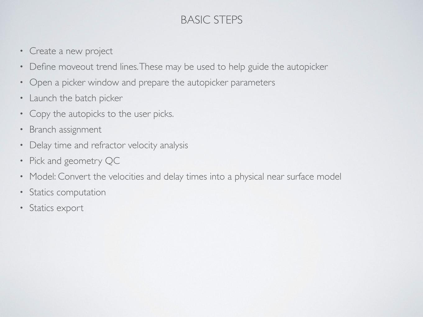
BASIC STEPS
• Create a new project • Define moveout trend lines. These may be used to help guide the autopicker • Open a picker window and prepare the autopicker parameters • Launch the batch picker • Copy the autopicks to the user picks. • Branch assignment • Delay time and refractor velocity analysis • Pick and geometry QC • Model: Convert the velocities and delay times into a physical near surface model • Statics computation • Statics export
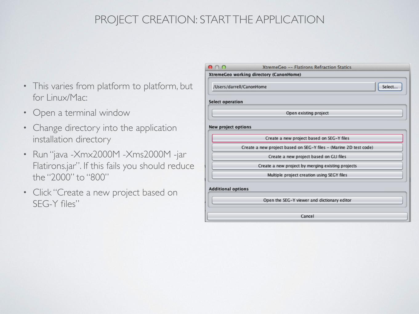
PROJECT CREATION: START THE APPLICATION
• This varies from platform to platform, but for Linux/Mac:
• Open a terminal window • Change directory into the application
installation directory • Run “java -Xmx2000M -Xms2000M -jar
Flatirons.jar”. If this fails you should reduce the “2000” to “800”
• Click “Create a new project based on SEG-Y files”
PROJECT CREATION: PROJECT CREATION WIZARD, PAGE 1
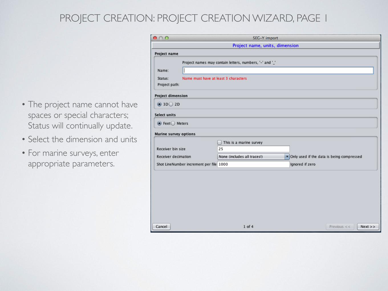
• The project name cannot have spaces or special characters; Status will continually update.
• Select the dimension and units • For marine surveys, enter
appropriate parameters.
PROJECT CREATION: PROJECT CREATION WIZARD, PAGE 2
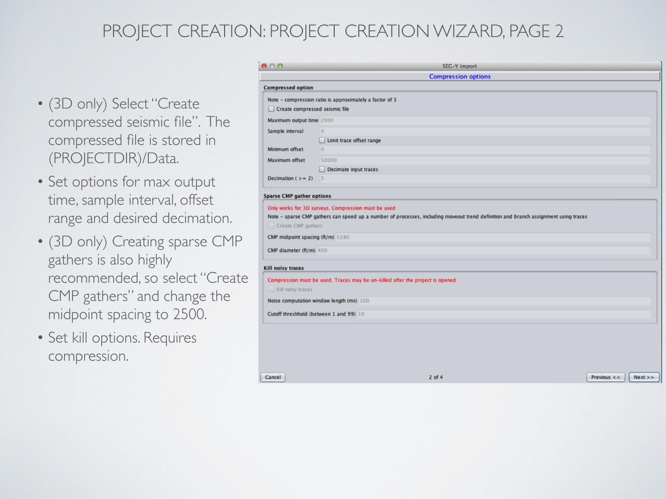
• (3D only) Select “Create compressed seismic file”. The compressed file is stored in (PROJECTDIR)/Data.
• Set options for max output time, sample interval, offset range and desired decimation.
• (3D only) Creating sparse CMP gathers is also highly recommended, so select “Create CMP gathers” and change the midpoint spacing to 2500.
• Set kill options. Requires compression.
PROJECT CREATION: PROJECT CREATION WIZARD, PAGE 3
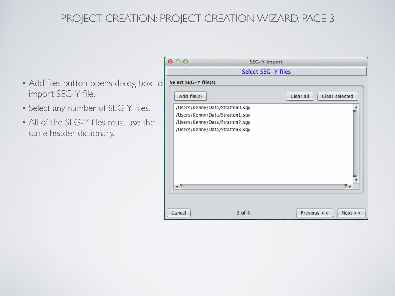
• Add files button opens dialog box to import SEG-Y file.
• Select any number of SEG-Y files. • All of the SEG-Y files must use the
same header dictionary.
PROJECT CREATION: PROJECT CREATION WIZARD, PAGE 4
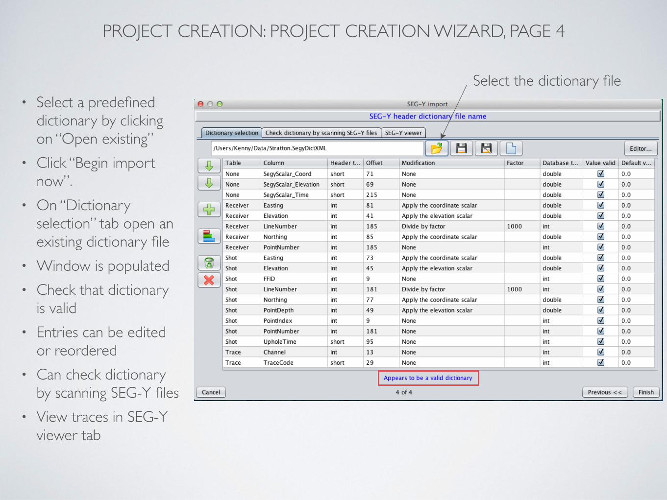
• Select a predefined dictionary by clicking on “Open existing”
• Click “Begin import now”.
• On “Dictionary selection” tab open an existing dictionary file
• Window is populated • Check that dictionary
is valid • Entries can be edited
or reordered • Can check dictionary
by scanning SEG-Y files • View traces in SEG-Y
viewer tab
Select the dictionary file
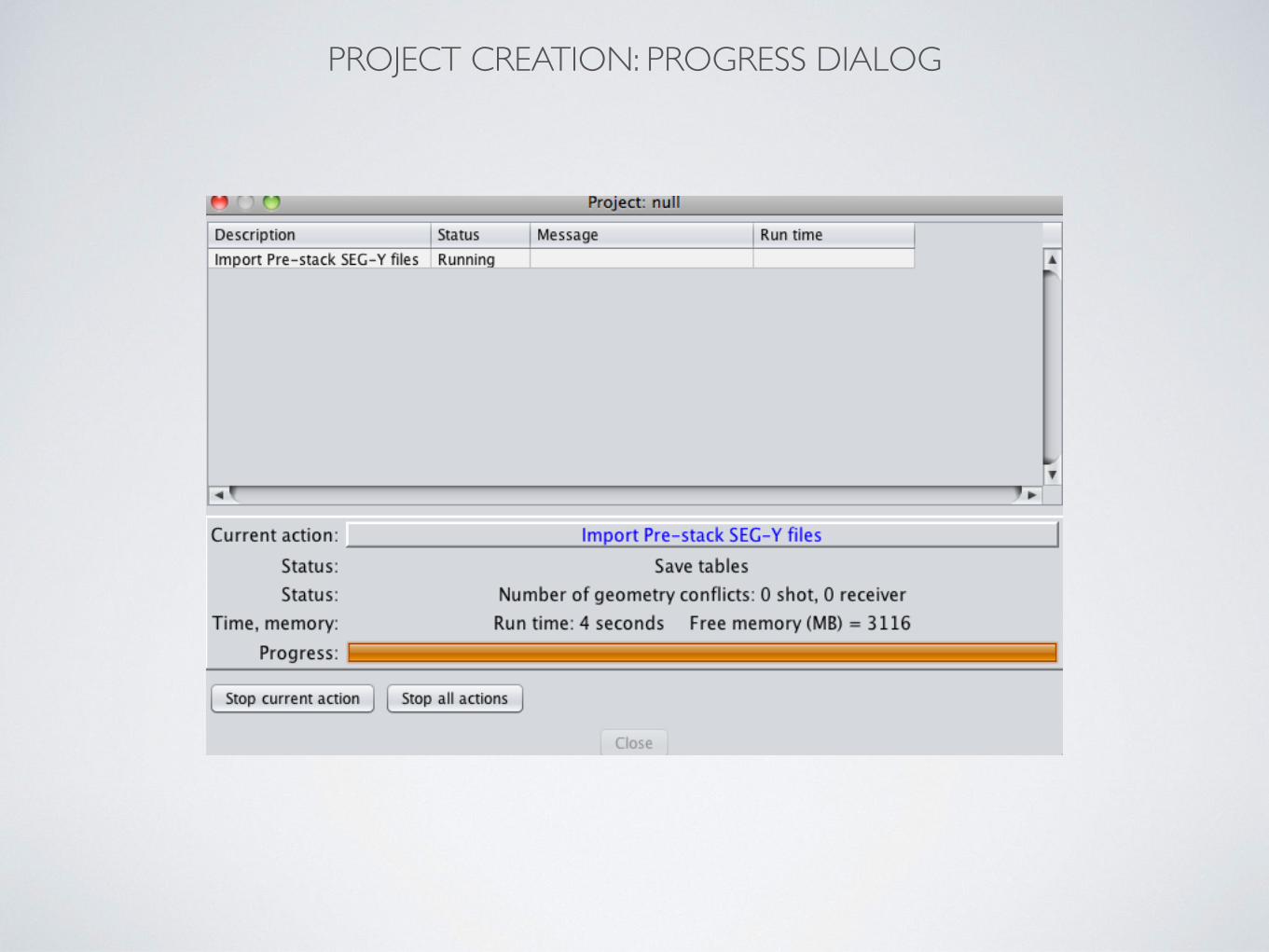
PROJECT CREATION: PROGRESS DIALOG
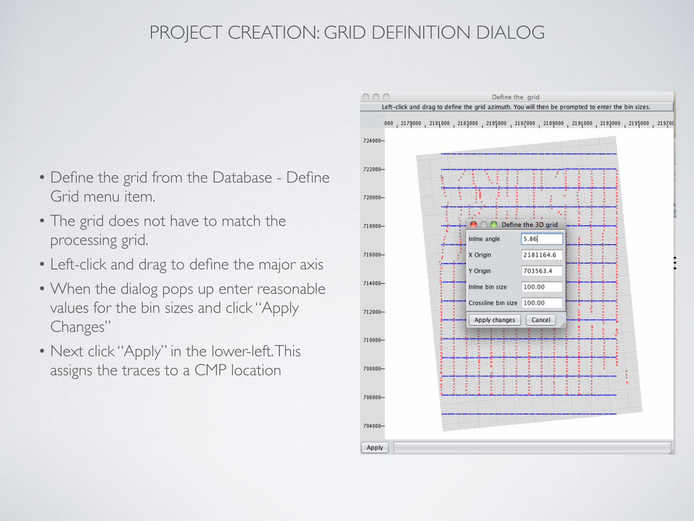
PROJECT CREATION: GRID DEFINITION DIALOG
• Define the grid from the Database - Define Grid menu item.
• The grid does not have to match the processing grid.
• Left-click and drag to define the major axis • When the dialog pops up enter reasonable
values for the bin sizes and click “Apply Changes”
• Next click “Apply” in the lower-left. This assigns the traces to a CMP location
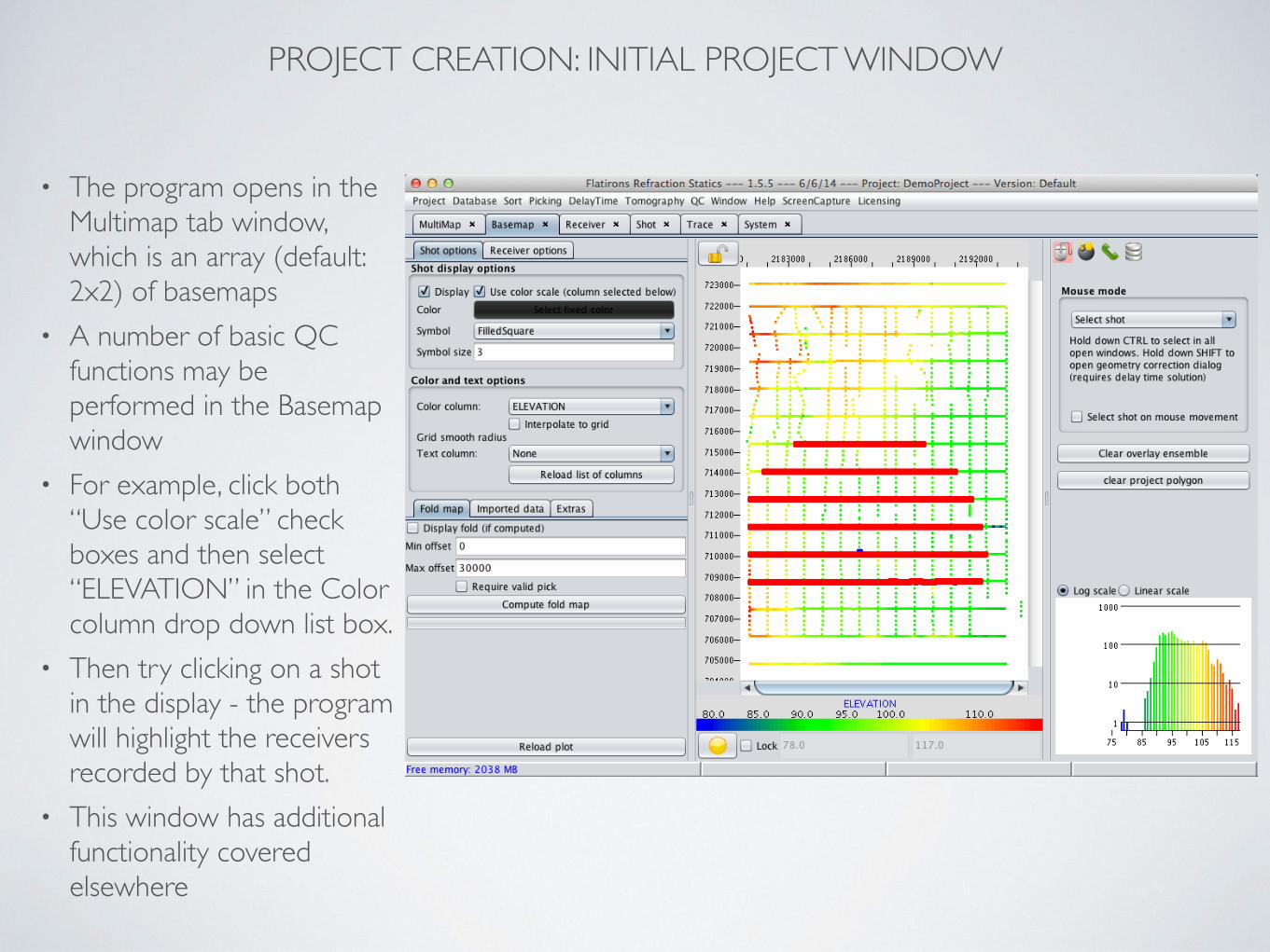
PROJECT CREATION: INITIAL PROJECT WINDOW
• The program opens in the Multimap tab window, which is an array (default: 2x2) of basemaps
• A number of basic QC functions may be performed in the Basemap window
• For example, click both “Use color scale” check boxes and then select “ELEVATION” in the Color column drop down list box.
• Then try clicking on a shot in the display - the program will highlight the receivers recorded by that shot.
• This window has additional functionality covered elsewhere
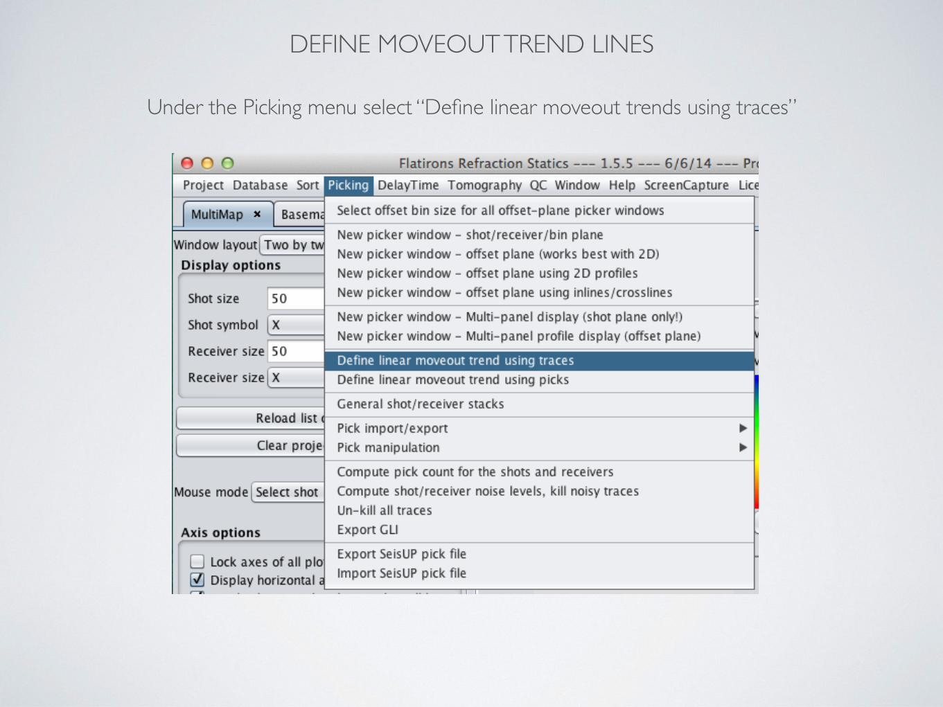
DEFINE MOVEOUT TREND LINES
Under the Picking menu select “Define linear moveout trends using traces”
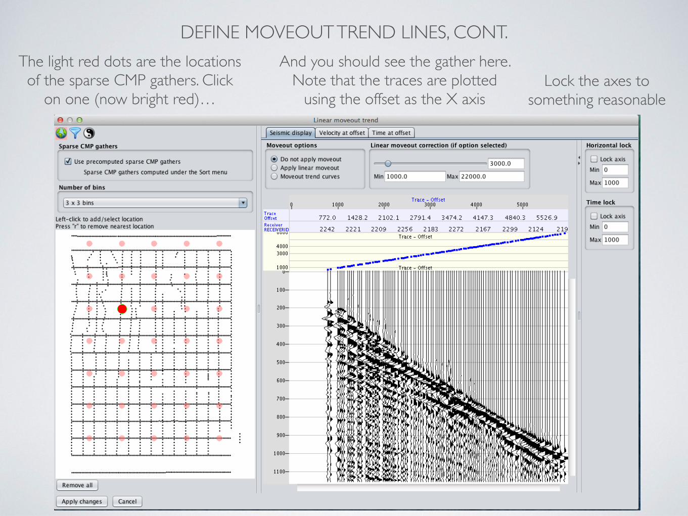
DEFINE MOVEOUT TREND LINES, CONT.The light red dots are the locations of the sparse CMP gathers. Click
on one (now bright red)…
And you should see the gather here. Note that the traces are plotted
using the offset as the X axisLock the axes to
something reasonable
DEFINE MOVEOUT TREND LINES, CONT.
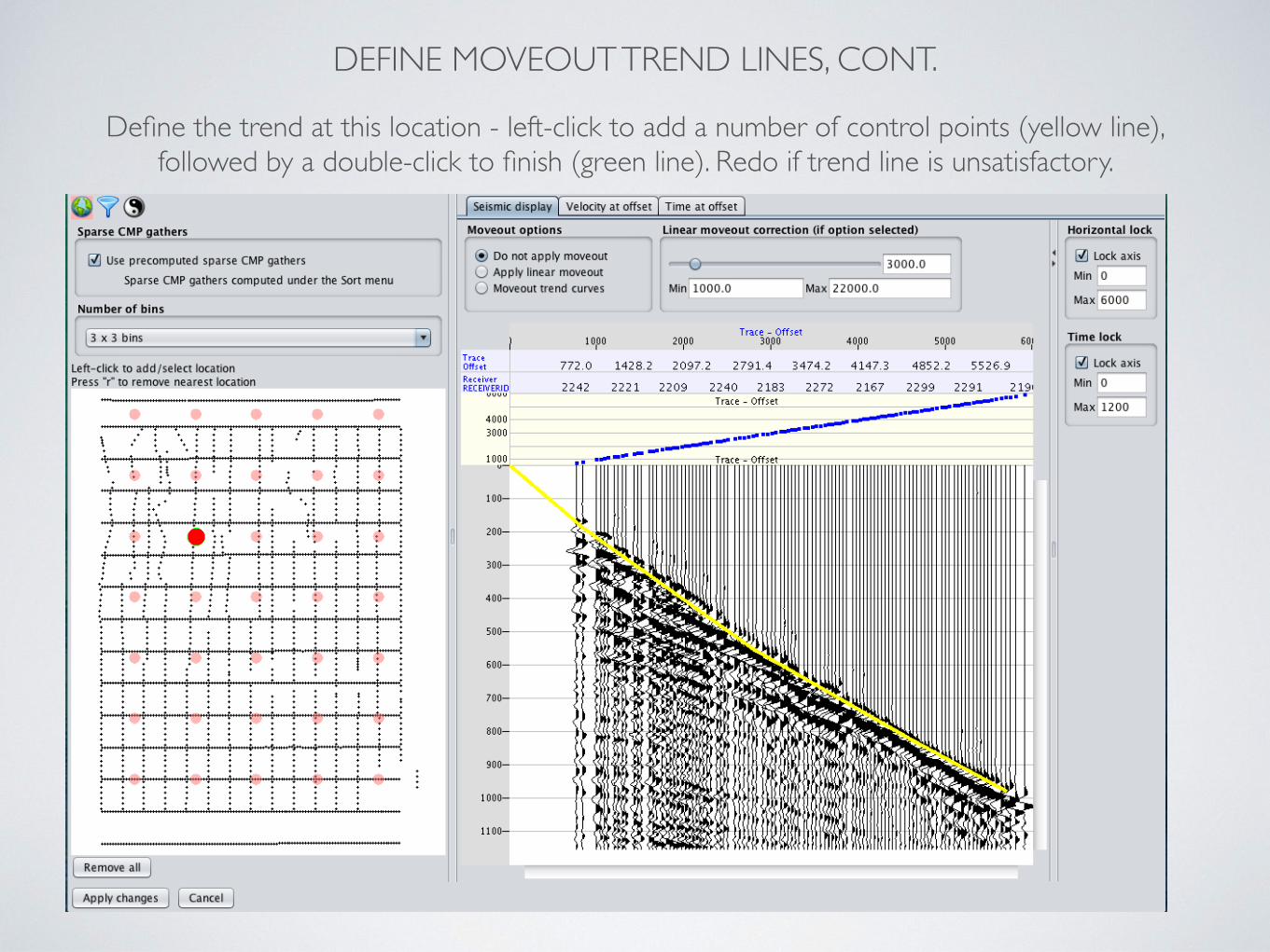
Define the trend at this location - left-click to add a number of control points (yellow line), followed by a double-click to finish (green line). Redo if trend line is unsatisfactory.
DEFINE MOVEOUT TREND LINES, CONT.
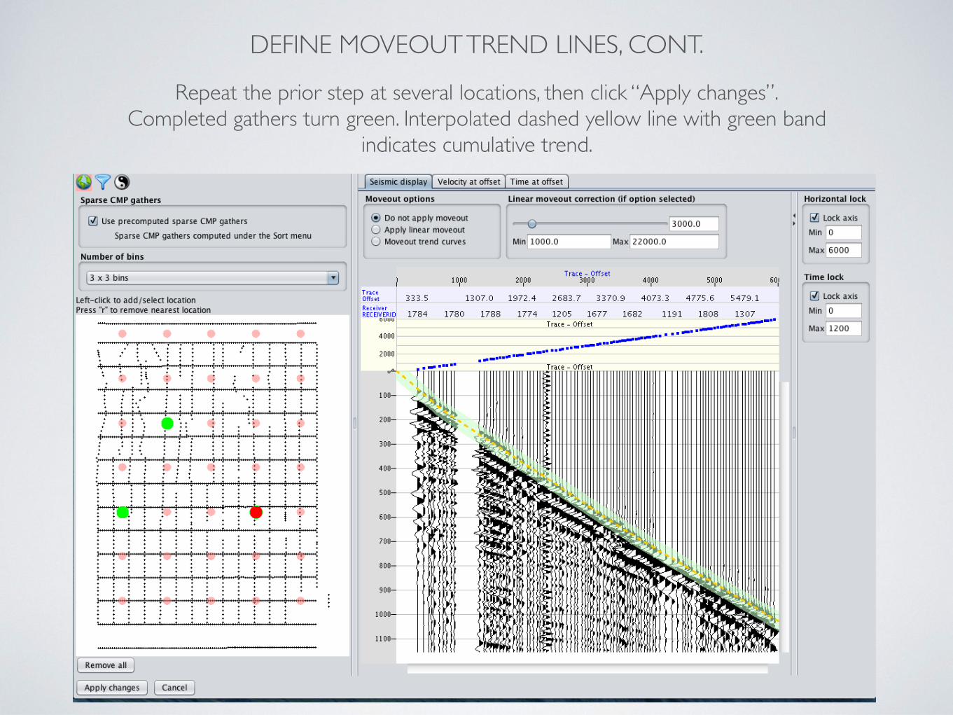
Repeat the prior step at several locations, then click “Apply changes”. Completed gathers turn green. Interpolated dashed yellow line with green band
indicates cumulative trend.
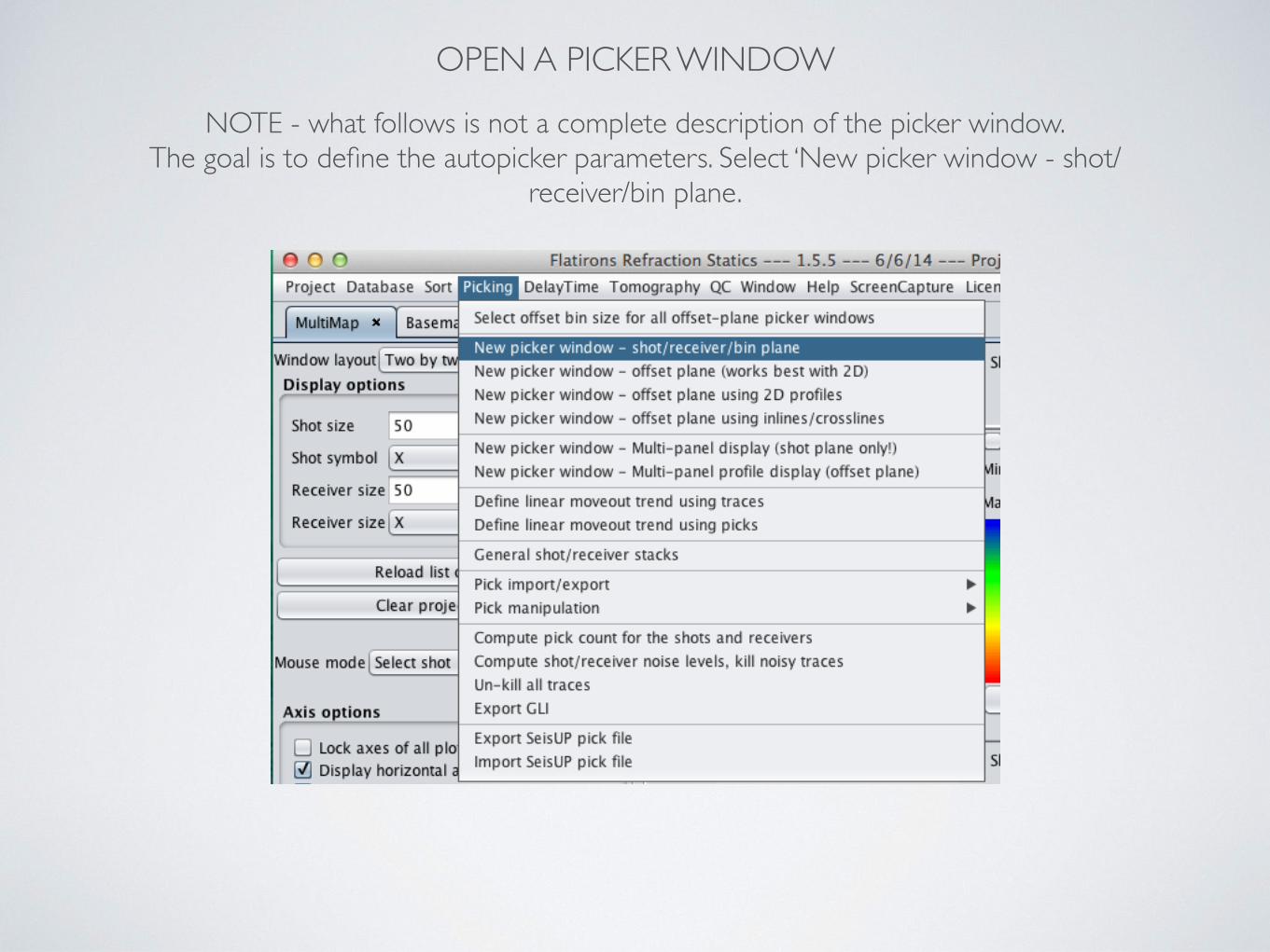
OPEN A PICKER WINDOW
NOTE - what follows is not a complete description of the picker window. The goal is to define the autopicker parameters. Select ‘New picker window - shot/
receiver/bin plane.
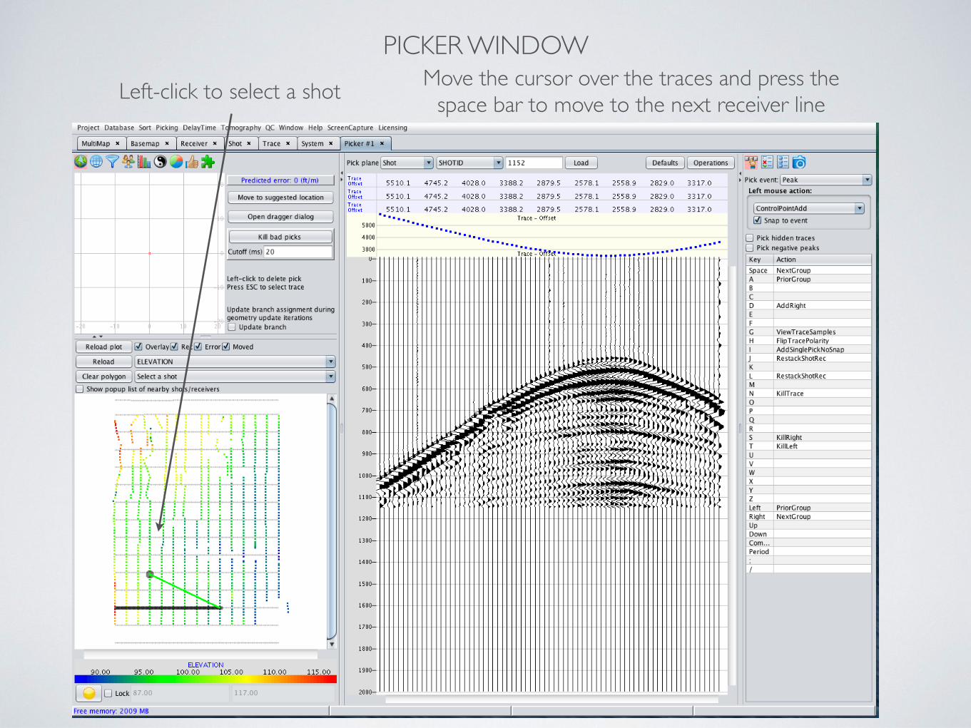
PICKER WINDOWLeft-click to select a shot Move the cursor over the traces and press the
space bar to move to the next receiver line
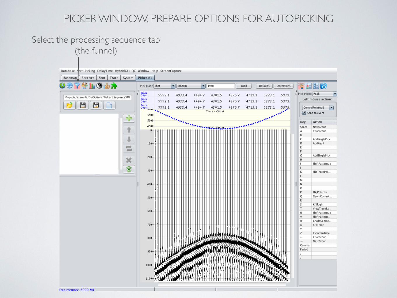
PICKER WINDOW, PREPARE OPTIONS FOR AUTOPICKING
Select the processing sequence tab (the funnel)
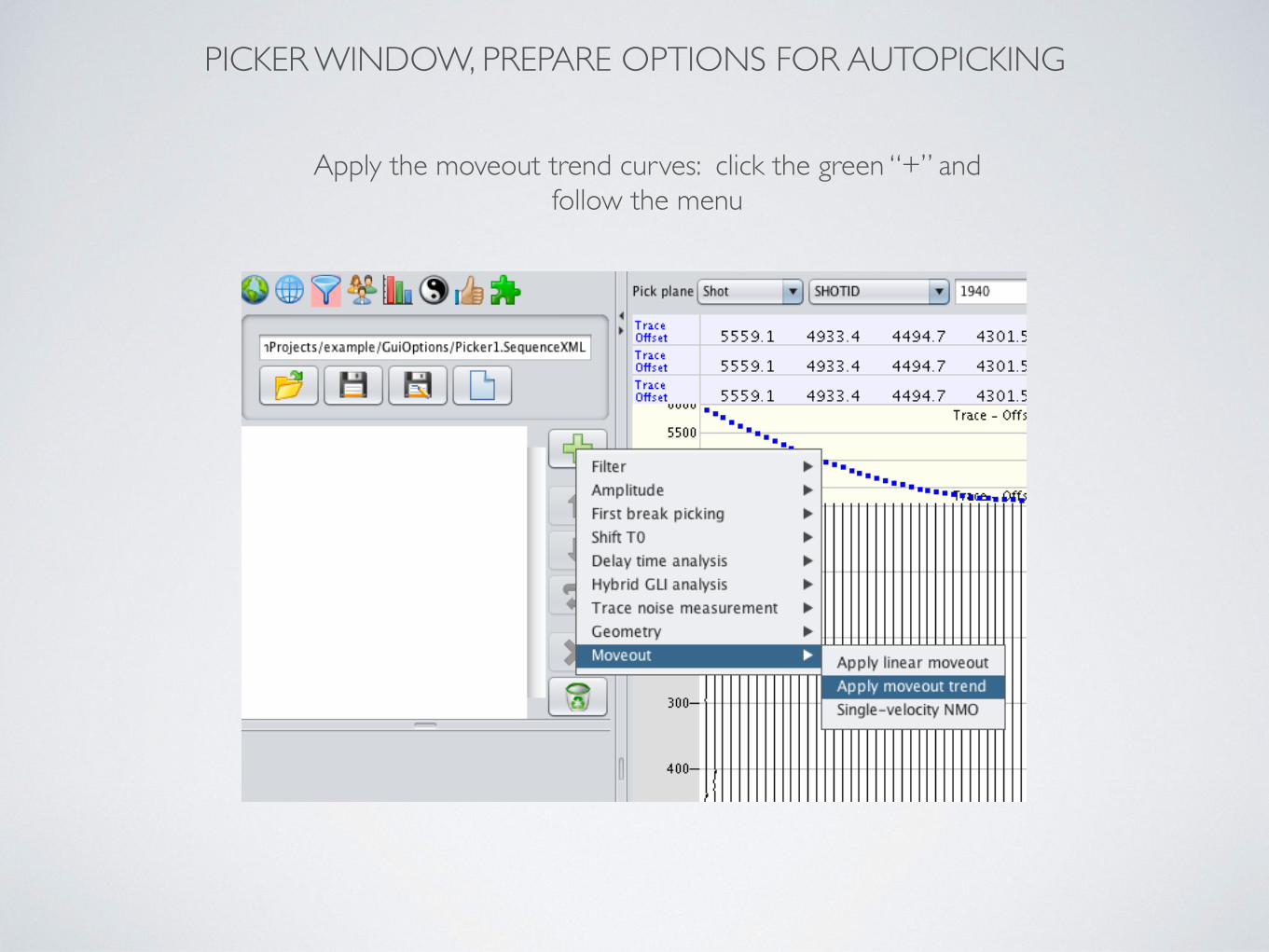
PICKER WINDOW, PREPARE OPTIONS FOR AUTOPICKING
Apply the moveout trend curves: click the green “+” and follow the menu
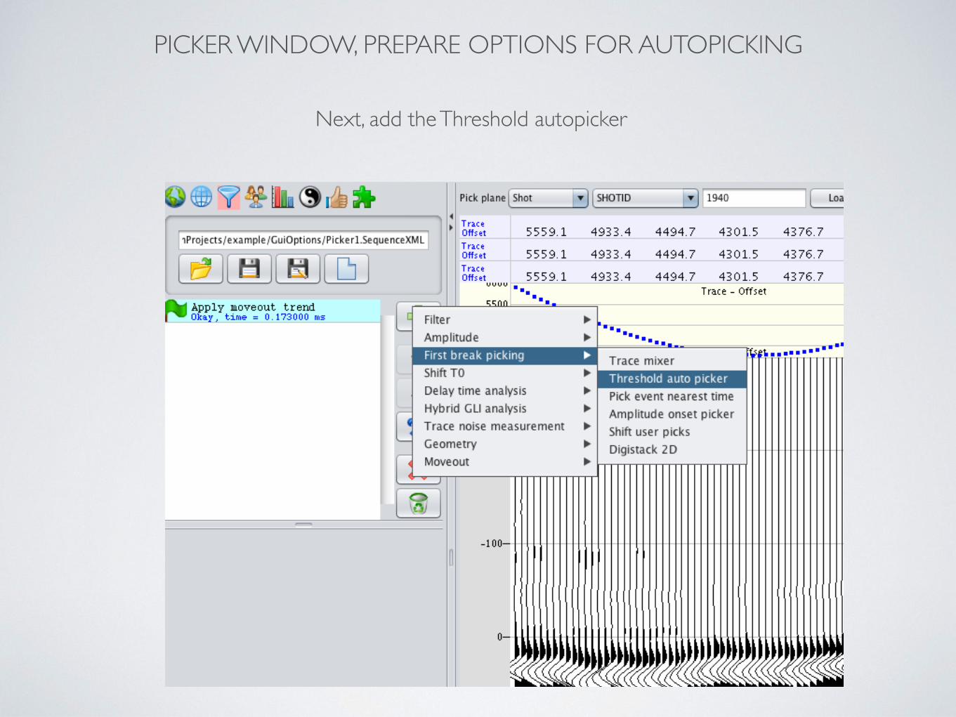
PICKER WINDOW, PREPARE OPTIONS FOR AUTOPICKING
Next, add the Threshold autopicker
PICKER WINDOW, PREPARE OPTIONS FOR AUTOPICKING
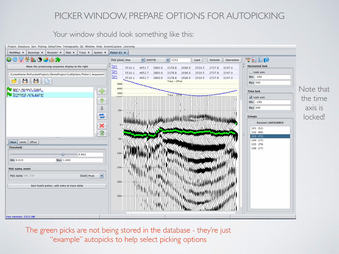
Your window should look something like this:
Note that the time axis is locked!
The green picks are not being stored in the database - they’re just “example” autopicks to help select picking options
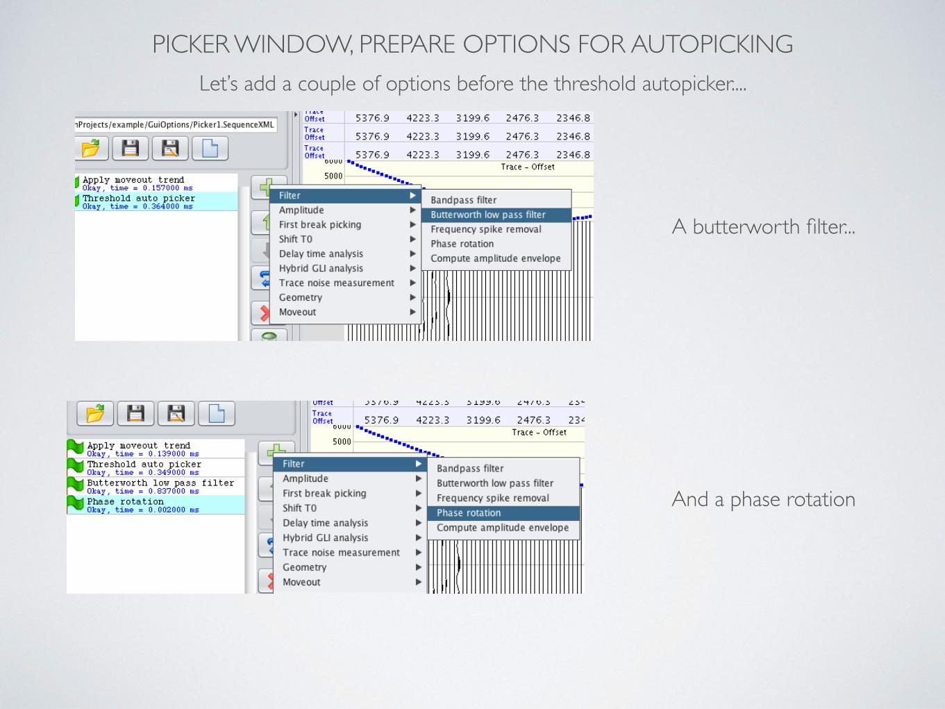
PICKER WINDOW, PREPARE OPTIONS FOR AUTOPICKINGLet’s add a couple of options before the threshold autopicker....
A butterworth filter...
And a phase rotation
PICKER WINDOW, PREPARE OPTIONS FOR AUTOPICKING
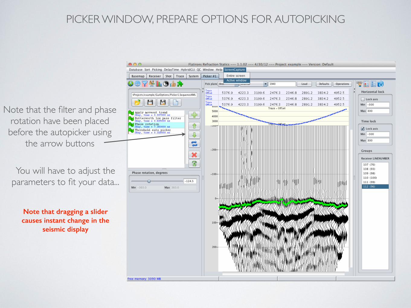
You will have to adjust the parameters to fit your data...
Note that the filter and phase rotation have been placed before the autopicker using
the arrow buttons
Note that dragging a slider causes instant change in the
seismic display
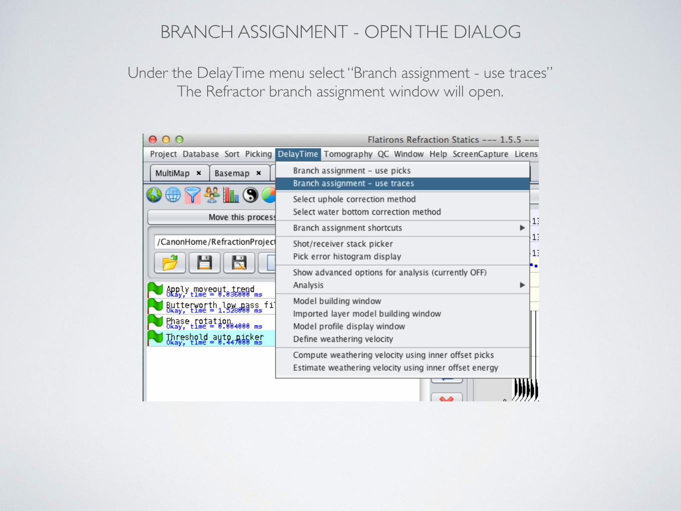
BRANCH ASSIGNMENT - OPEN THE DIALOG
Under the DelayTime menu select “Branch assignment - use traces” The Refractor branch assignment window will open.
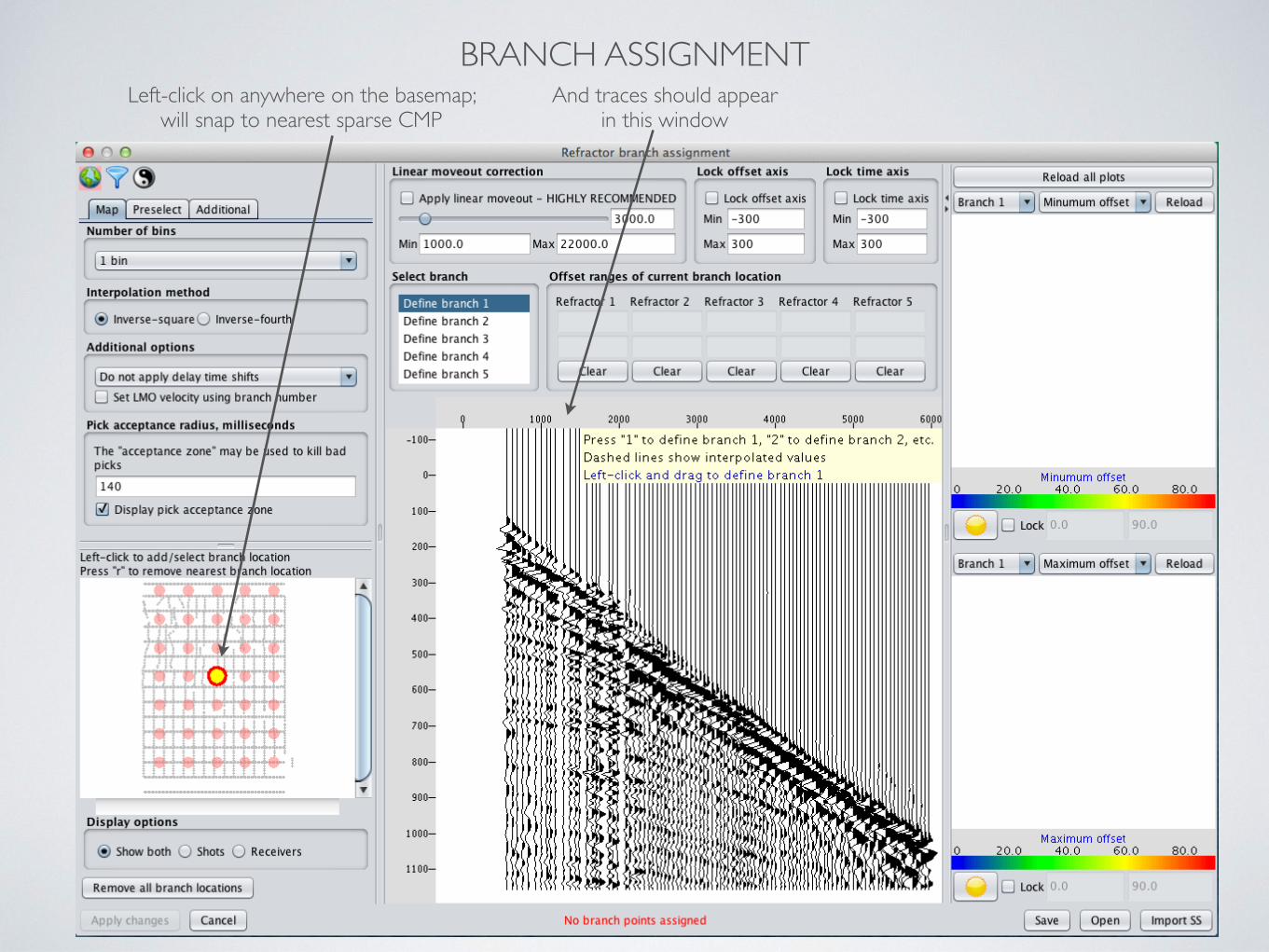
BRANCH ASSIGNMENTLeft-click on anywhere on the basemap;
will snap to nearest sparse CMPAnd traces should appear
in this window
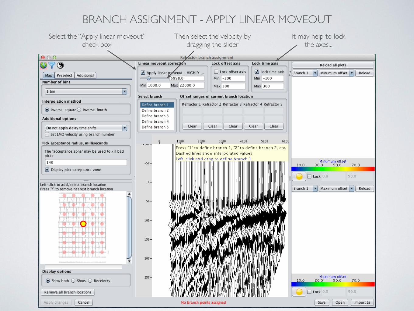
BRANCH ASSIGNMENT - APPLY LINEAR MOVEOUTSelect the “Apply linear moveout”
check boxThen select the velocity by
dragging the sliderIt may help to lock
the axes...
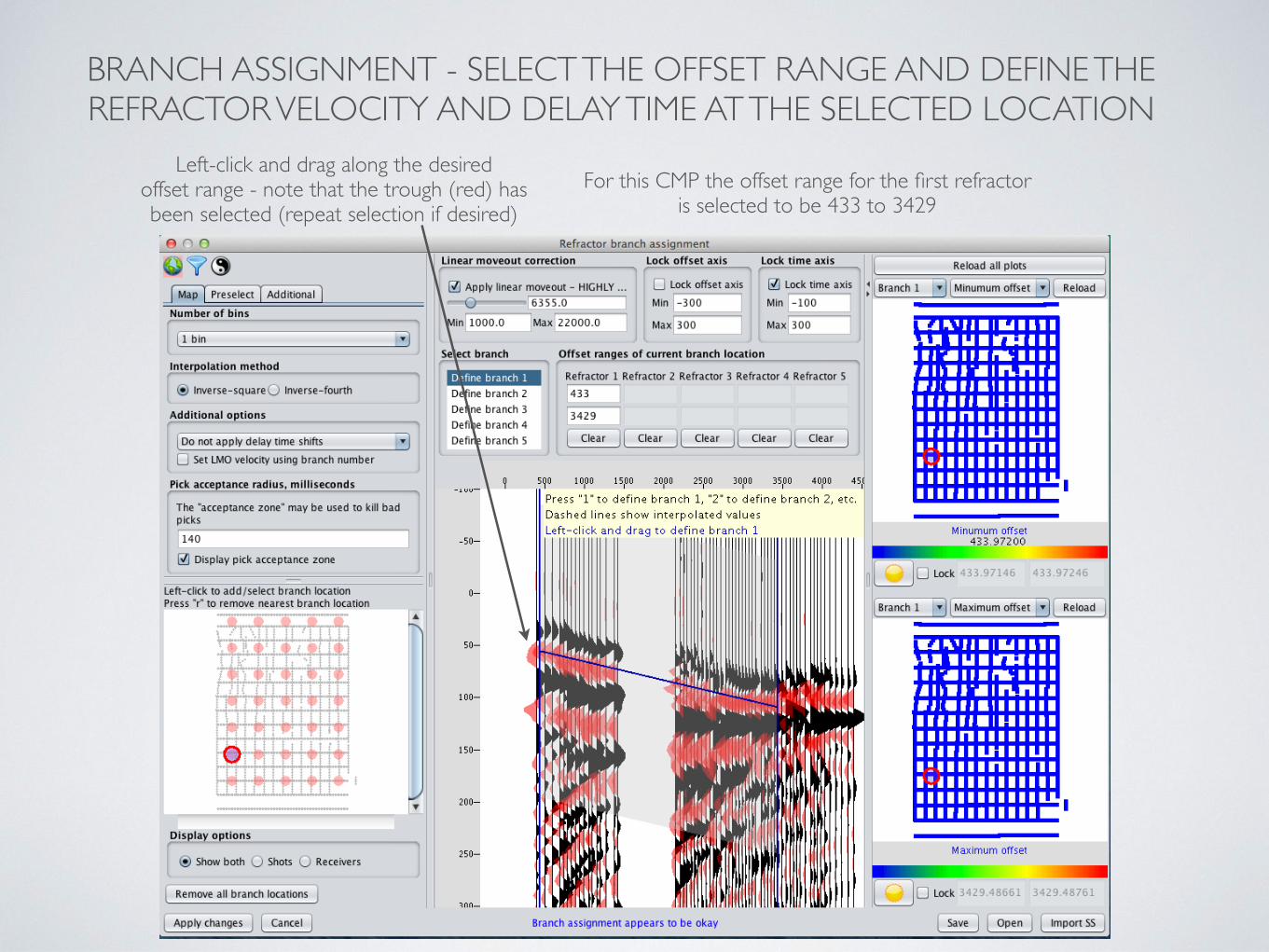
BRANCH ASSIGNMENT - SELECT THE OFFSET RANGE AND DEFINE THE REFRACTOR VELOCITY AND DELAY TIME AT THE SELECTED LOCATION
Left-click and drag along the desired offset range - note that the trough (red) has been selected (repeat selection if desired)
For this CMP the offset range for the first refractor is selected to be 433 to 3429
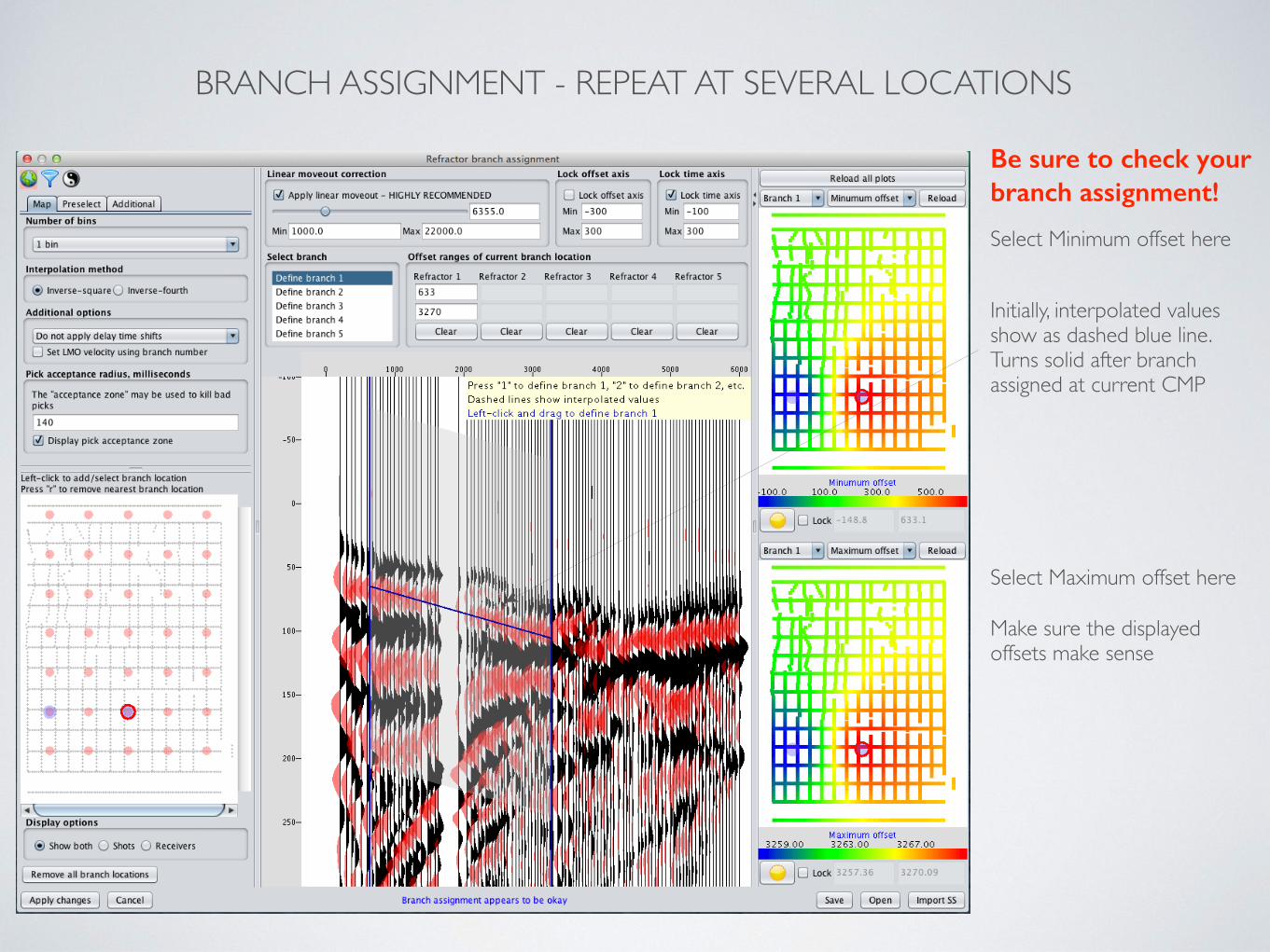
BRANCH ASSIGNMENT - REPEAT AT SEVERAL LOCATIONS
Be sure to check your branch assignment!
Select Minimum offset here
Select Maximum offset here
Make sure the displayed offsets make sense
Initially, interpolated values show as dashed blue line. Turns solid after branch assigned at current CMP
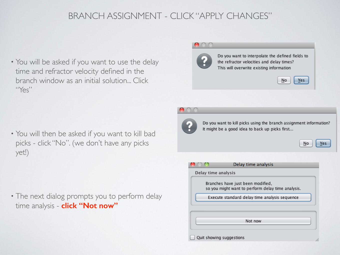
BRANCH ASSIGNMENT - CLICK “APPLY CHANGES”
• You will be asked if you want to use the delay time and refractor velocity defined in the branch window as an initial solution... Click “Yes”
!
• You will then be asked if you want to kill bad picks - click “No”. (we don’t have any picks yet!)
!
• The next dialog prompts you to perform delay time analysis - click “Not now”
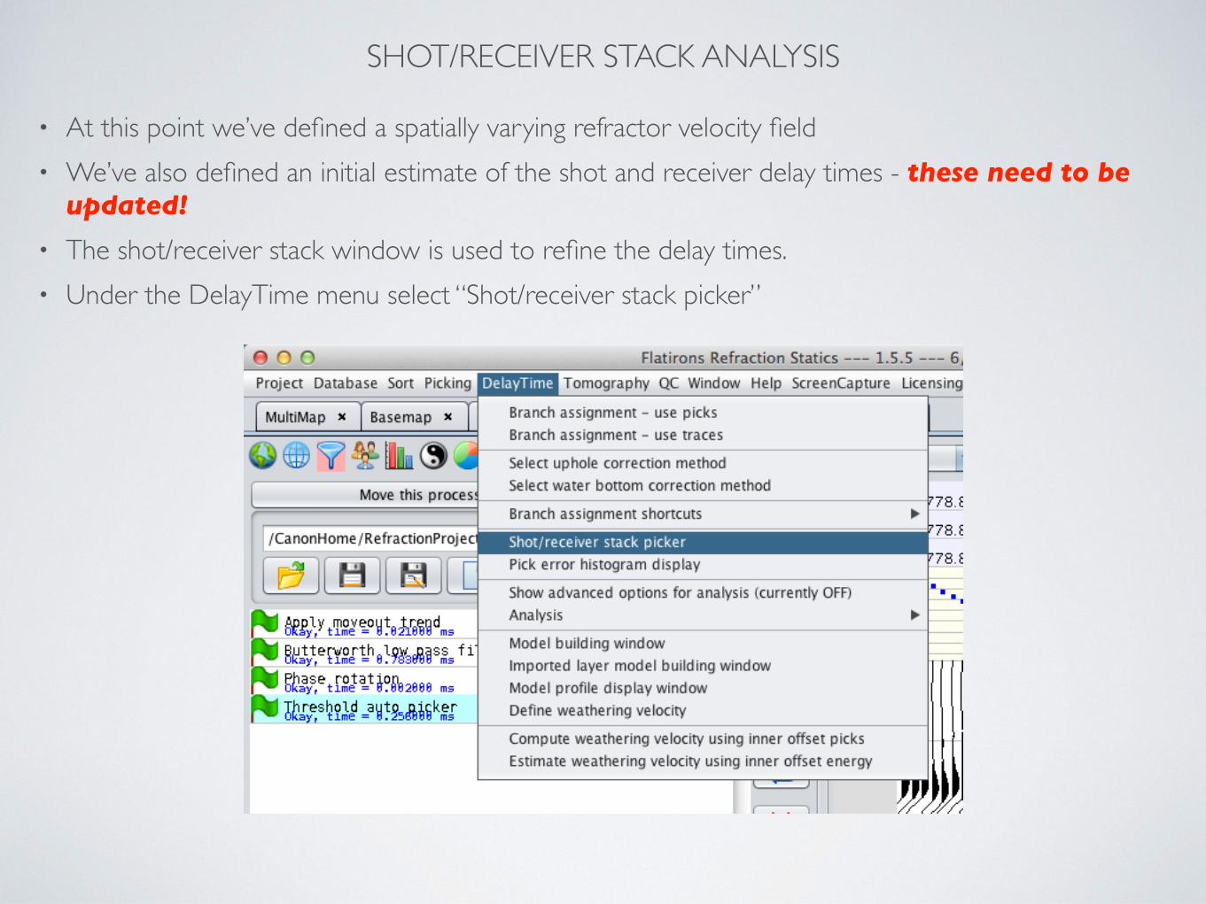
SHOT/RECEIVER STACK ANALYSIS
• At this point we’ve defined a spatially varying refractor velocity field • We’ve also defined an initial estimate of the shot and receiver delay times - these need to be
updated! • The shot/receiver stack window is used to refine the delay times. • Under the DelayTime menu select “Shot/receiver stack picker”
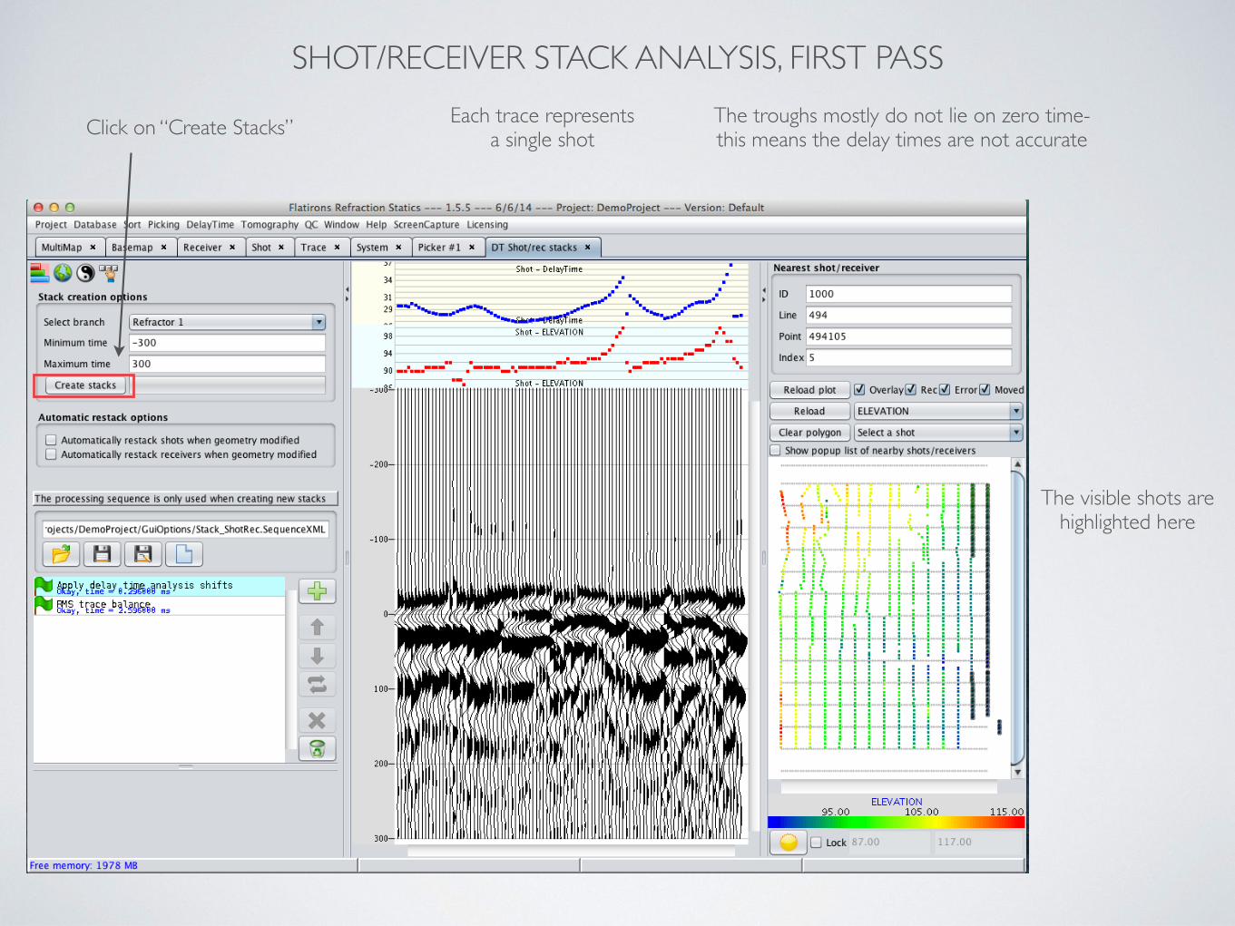
SHOT/RECEIVER STACK ANALYSIS, FIRST PASS
Click on “Create Stacks” Each trace represents a single shot
The troughs mostly do not lie on zero time- this means the delay times are not accurate
The visible shots are highlighted here
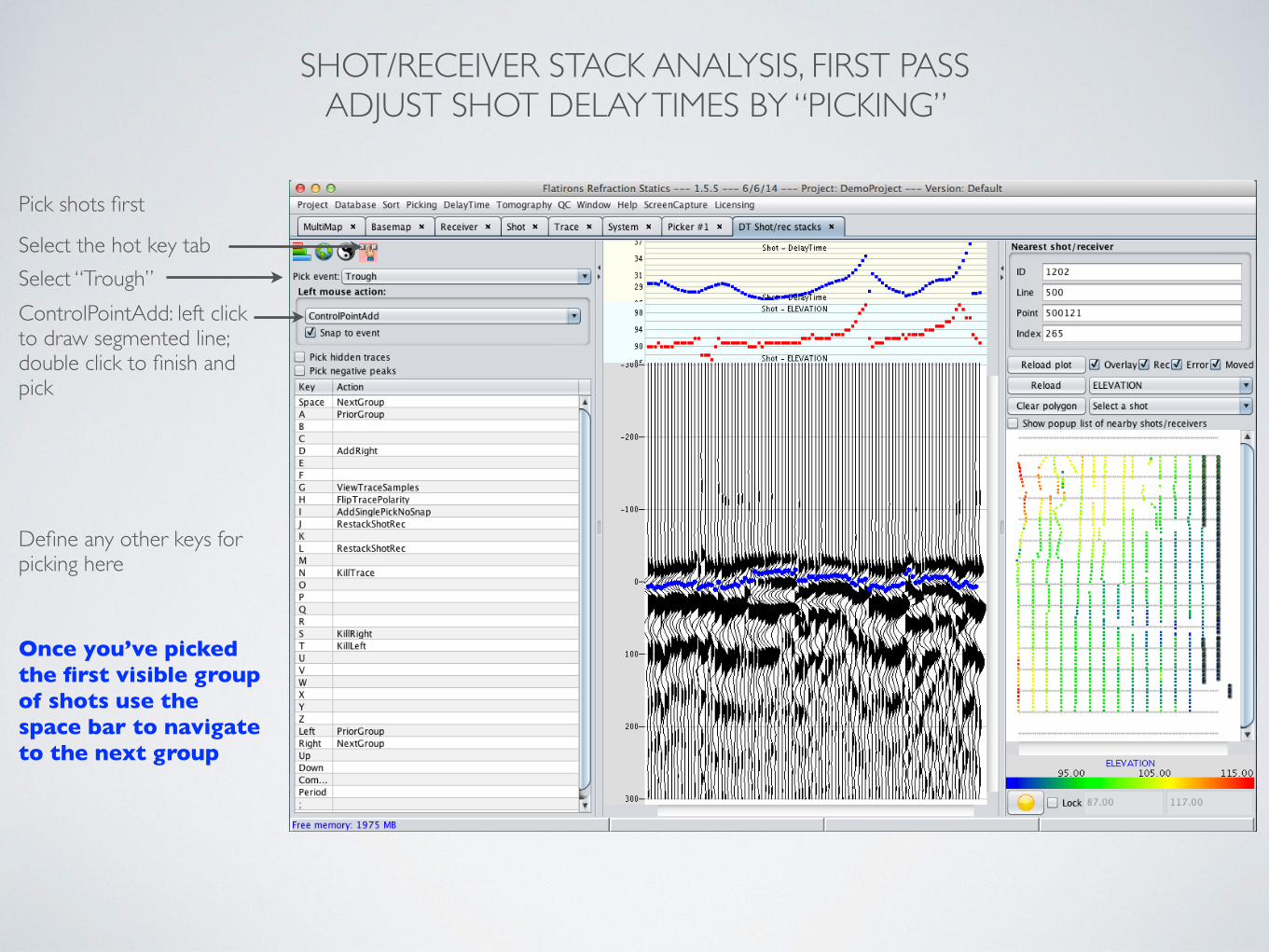
SHOT/RECEIVER STACK ANALYSIS, FIRST PASS ADJUST SHOT DELAY TIMES BY “PICKING”
Select the hot key tabSelect “Trough”ControlPointAdd: left click to draw segmented line; double click to finish and pick
Define any other keys for picking here
Once you’ve picked the first visible group of shots use the space bar to navigate to the next group
Pick shots first
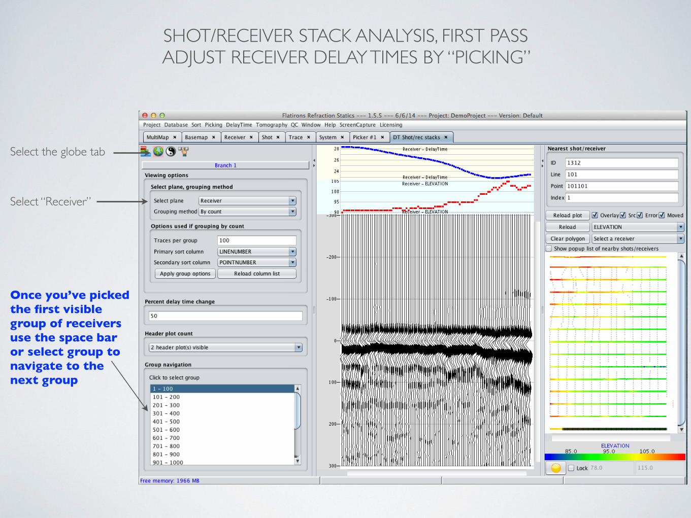
SHOT/RECEIVER STACK ANALYSIS, FIRST PASS ADJUST RECEIVER DELAY TIMES BY “PICKING”
Select the globe tab
Select “Receiver”
Once you’ve picked the first visible group of receivers use the space bar or select group to navigate to the next group
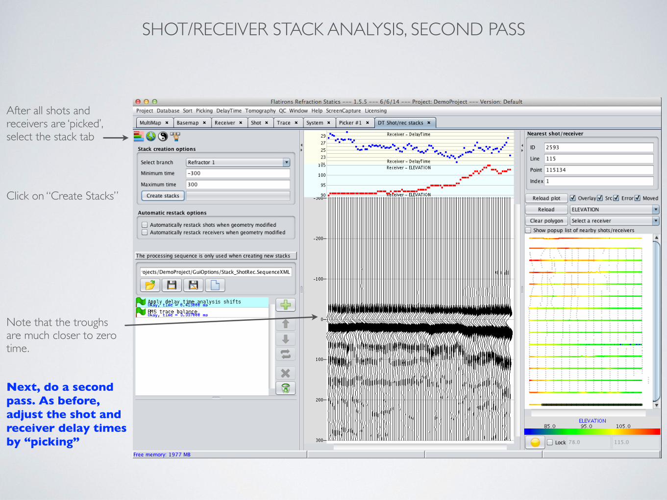
SHOT/RECEIVER STACK ANALYSIS, SECOND PASS
Click on “Create Stacks”
Note that the troughs are much closer to zero time.
Next, do a second pass. As before, adjust the shot and receiver delay times by “picking”
After all shots and receivers are ‘picked’, select the stack tab
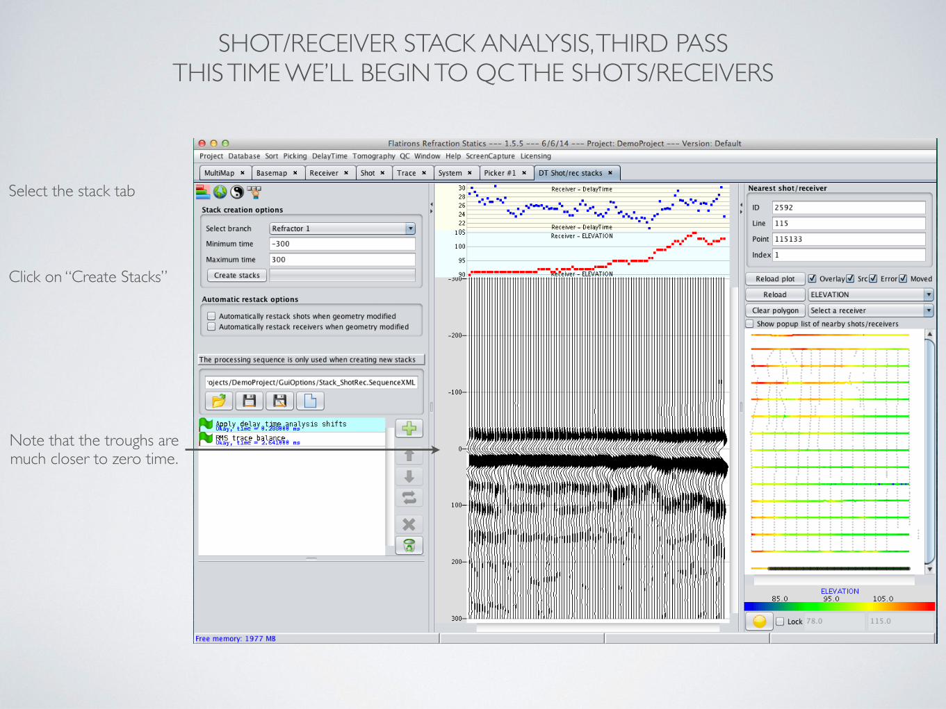
SHOT/RECEIVER STACK ANALYSIS, THIRD PASS THIS TIME WE’LL BEGIN TO QC THE SHOTS/RECEIVERS
Click on “Create Stacks”
Select the stack tab
Note that the troughs are much closer to zero time.
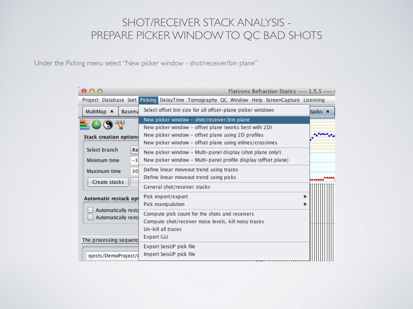
SHOT/RECEIVER STACK ANALYSIS - PREPARE PICKER WINDOW TO QC BAD SHOTS
Under the Picking menu select “New picker window - shot/receiver/bin plane”
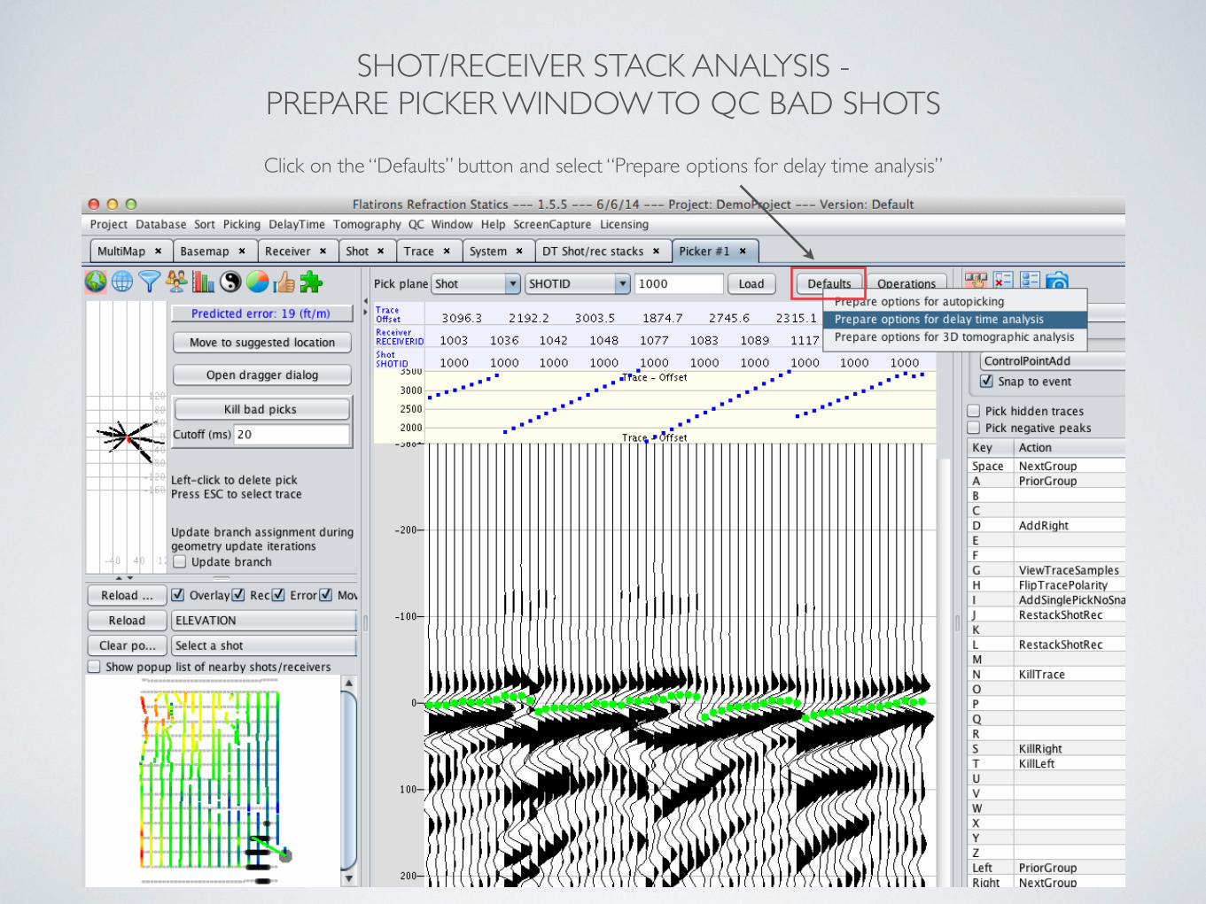
SHOT/RECEIVER STACK ANALYSIS - PREPARE PICKER WINDOW TO QC BAD SHOTS
Click on the “Defaults” button and select “Prepare options for delay time analysis”
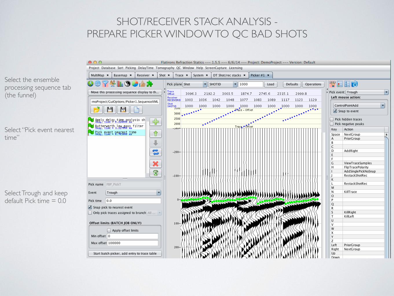
SHOT/RECEIVER STACK ANALYSIS - PREPARE PICKER WINDOW TO QC BAD SHOTS
Select the ensemble processing sequence tab (the funnel)
Select “Pick event nearest time”
Select Trough and keep default Pick time = 0.0
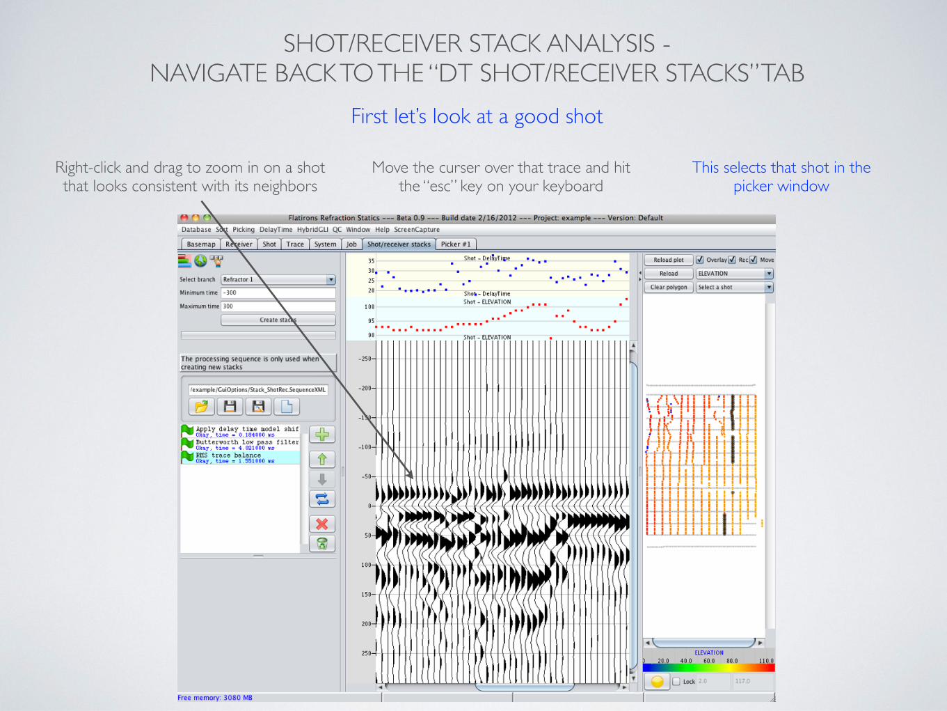
SHOT/RECEIVER STACK ANALYSIS - NAVIGATE BACK TO THE “DT SHOT/RECEIVER STACKS” TAB
Right-click and drag to zoom in on a shot that looks consistent with its neighbors
Move the curser over that trace and hit the “esc” key on your keyboard
This selects that shot in the picker window
First let’s look at a good shot
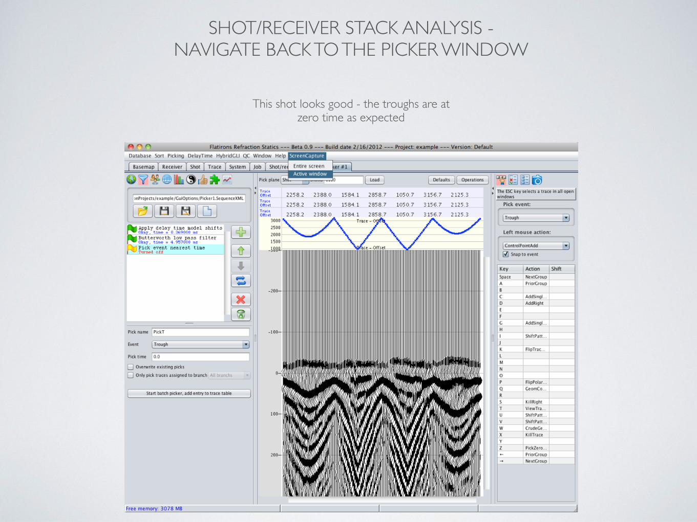
SHOT/RECEIVER STACK ANALYSIS - NAVIGATE BACK TO THE PICKER WINDOW
This shot looks good - the troughs are at zero time as expected
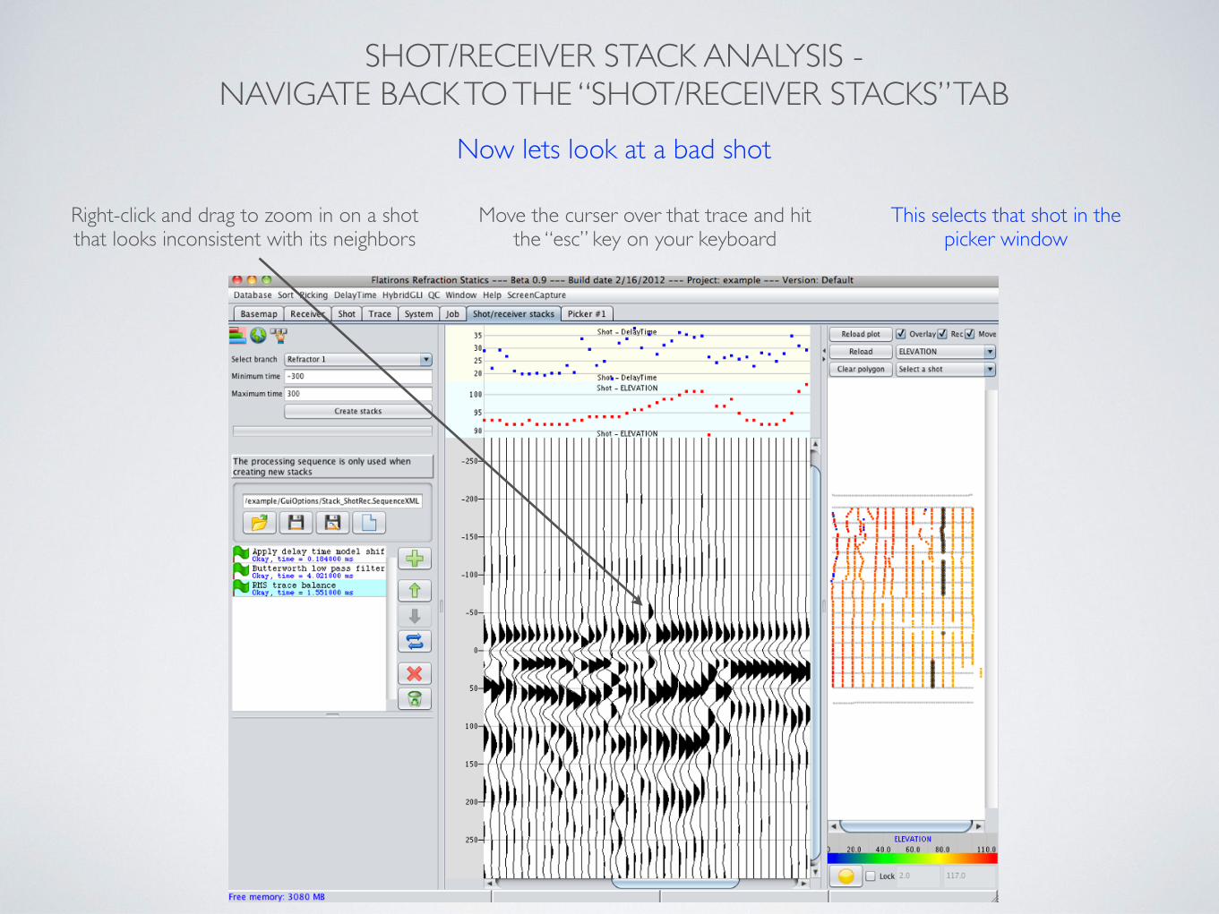
SHOT/RECEIVER STACK ANALYSIS - NAVIGATE BACK TO THE “SHOT/RECEIVER STACKS” TAB
Right-click and drag to zoom in on a shot that looks inconsistent with its neighbors
Move the curser over that trace and hit the “esc” key on your keyboard
This selects that shot in the picker window
Now lets look at a bad shot
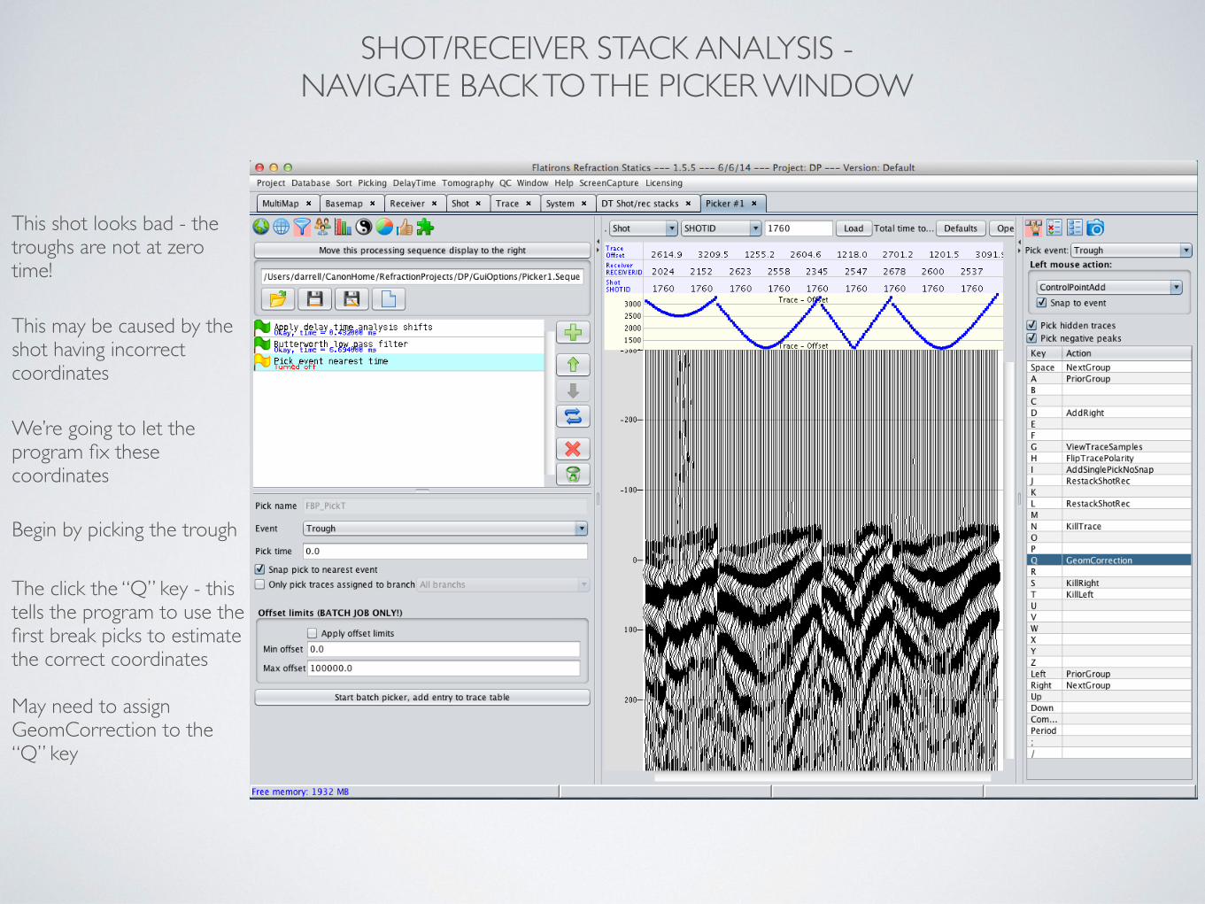
SHOT/RECEIVER STACK ANALYSIS - NAVIGATE BACK TO THE PICKER WINDOW
This shot looks bad - the troughs are not at zero time!
This may be caused by the shot having incorrect coordinates
We’re going to let the program fix these coordinates
Begin by picking the trough
The click the “Q” key - this tells the program to use the first break picks to estimate the correct coordinates
May need to assign GeomCorrection to the “Q” key
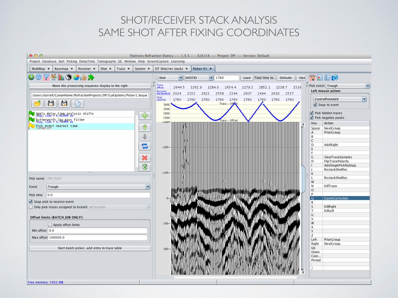
SHOT/RECEIVER STACK ANALYSIS SAME SHOT AFTER FIXING COORDINATES
SHOT/RECEIVER STACK ANALYSIS
• Repeat the following as needed ✴ Click on “Create stacks” in the shot/receiver stack window ✴ Scan through the shots and receivers ✴ Adjust delay times by picking ✴ Repair geometry using the picker window
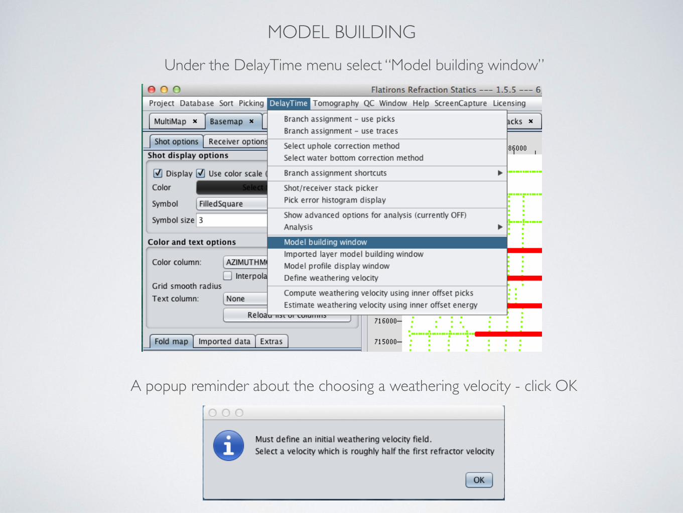
MODEL BUILDINGUnder the DelayTime menu select “Model building window”
A popup reminder about the choosing a weathering velocity - click OK
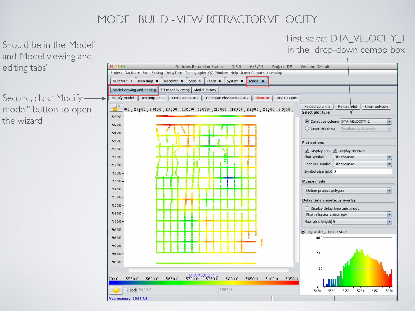
MODEL BUILD - VIEW REFRACTOR VELOCITYFirst, select DTA_VELOCITY_1 in the drop-down combo box
Second, click “Modify model” button to open the wizard
Should be in the ‘Model’ and ‘Model viewing and editing tabs’
MODEL BUILD - SET WEATHERING VELOCITY
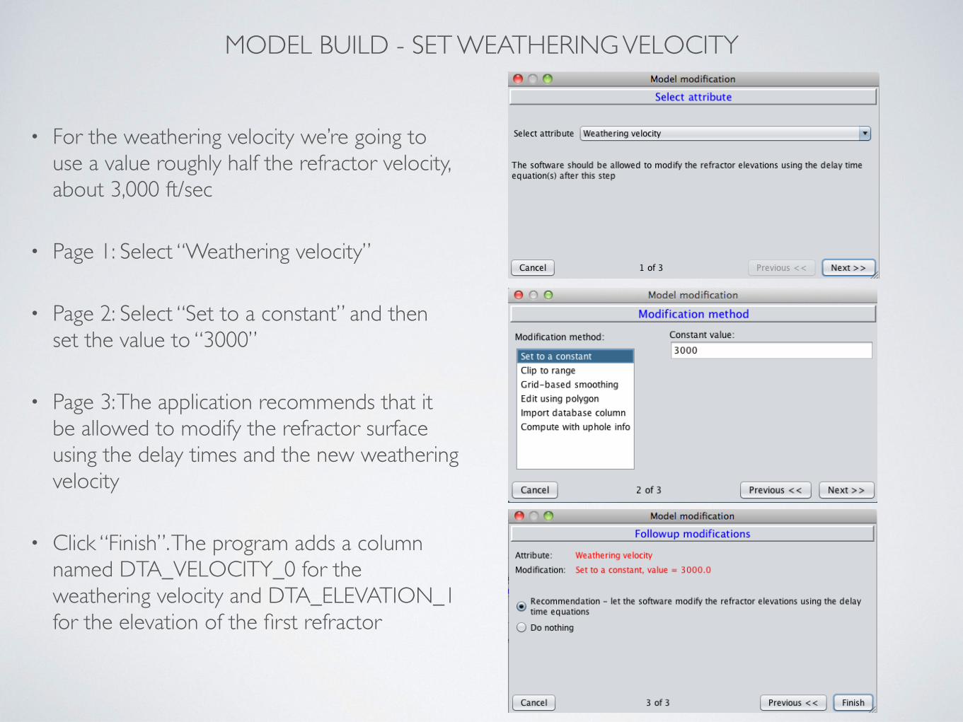
• For the weathering velocity we’re going to use a value roughly half the refractor velocity, about 3,000 ft/sec
• Page 1: Select “Weathering velocity”
• Page 2: Select “Set to a constant” and then set the value to “3000”
• Page 3: The application recommends that it be allowed to modify the refractor surface using the delay times and the new weathering velocity
• Click “Finish”. The program adds a column named DTA_VELOCITY_0 for the weathering velocity and DTA_ELEVATION_1 for the elevation of the first refractor
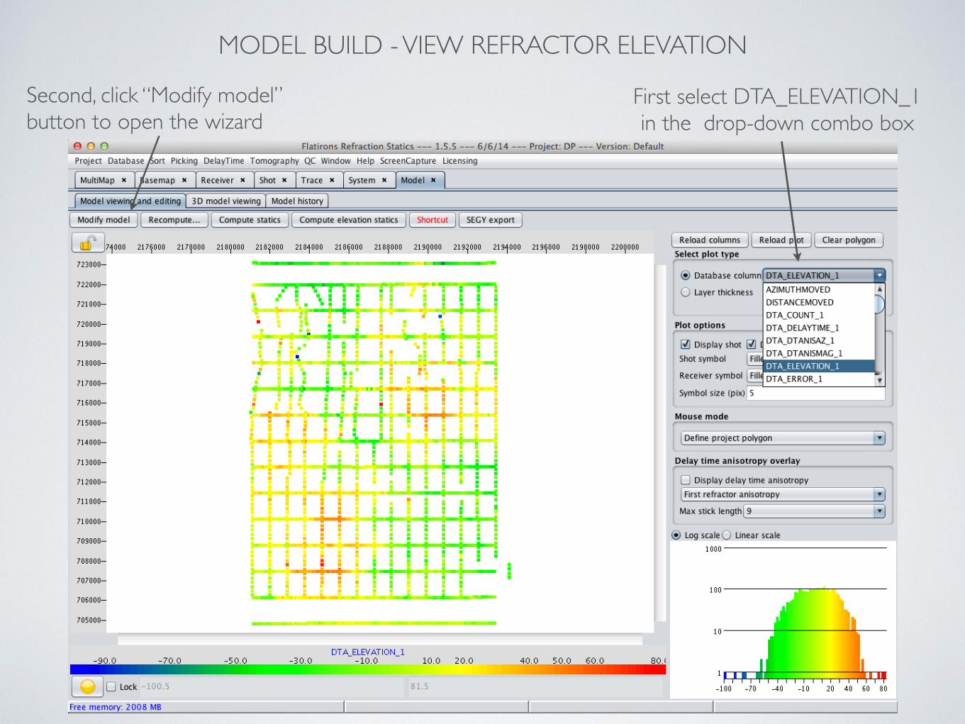
MODEL BUILD - VIEW REFRACTOR ELEVATION
First select DTA_ELEVATION_1 in the drop-down combo box
Second, click “Modify model” button to open the wizard

MODEL BUILD - SMOOTH REFRACTOR ELEVATION
• Page 1: Select “Refractor 1 elevation”
• Page 2: Select “Grid-based smoothing” and then select a radius of 1,000 feet.
• Page 3: The program recommends that it be allowed to modify the weathering velocity using the new refractor elevation and the delay times
• Click “Finish”
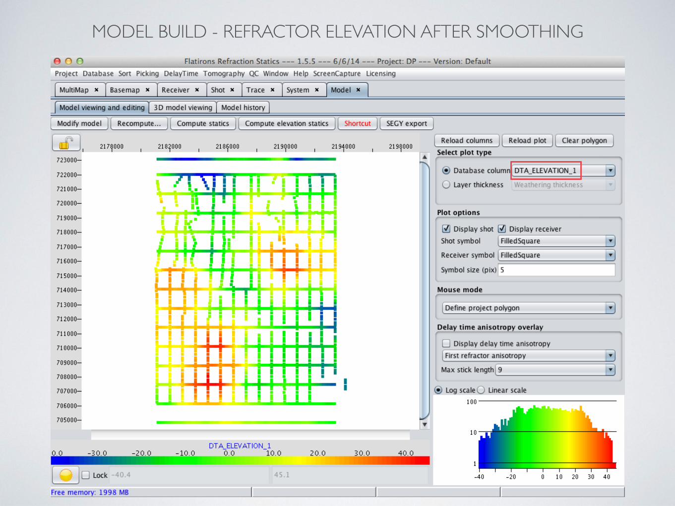
MODEL BUILD - REFRACTOR ELEVATION AFTER SMOOTHING
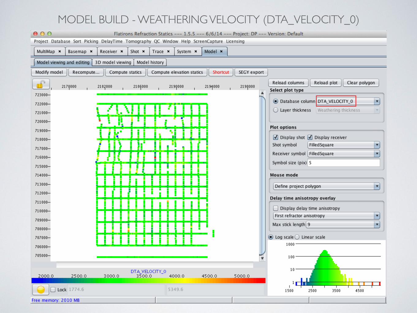
MODEL BUILD - WEATHERING VELOCITY (DTA_VELOCITY_0)
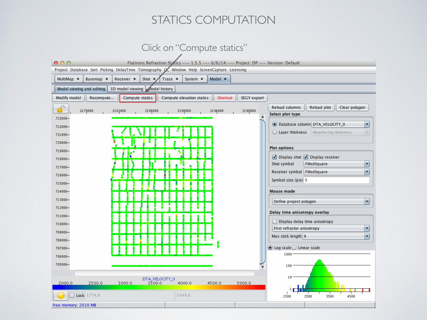
STATICS COMPUTATION
Click on “Compute statics”
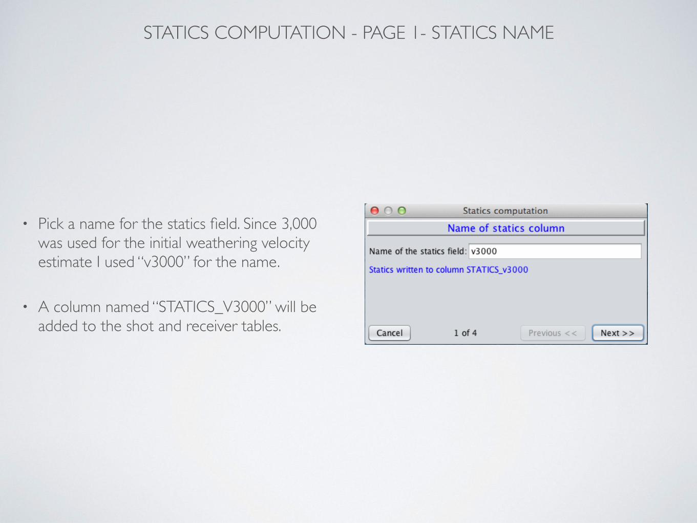
STATICS COMPUTATION - PAGE 1- STATICS NAME
• Pick a name for the statics field. Since 3,000 was used for the initial weathering velocity estimate I used “v3000” for the name.
• A column named “STATICS_V3000” will be added to the shot and receiver tables.
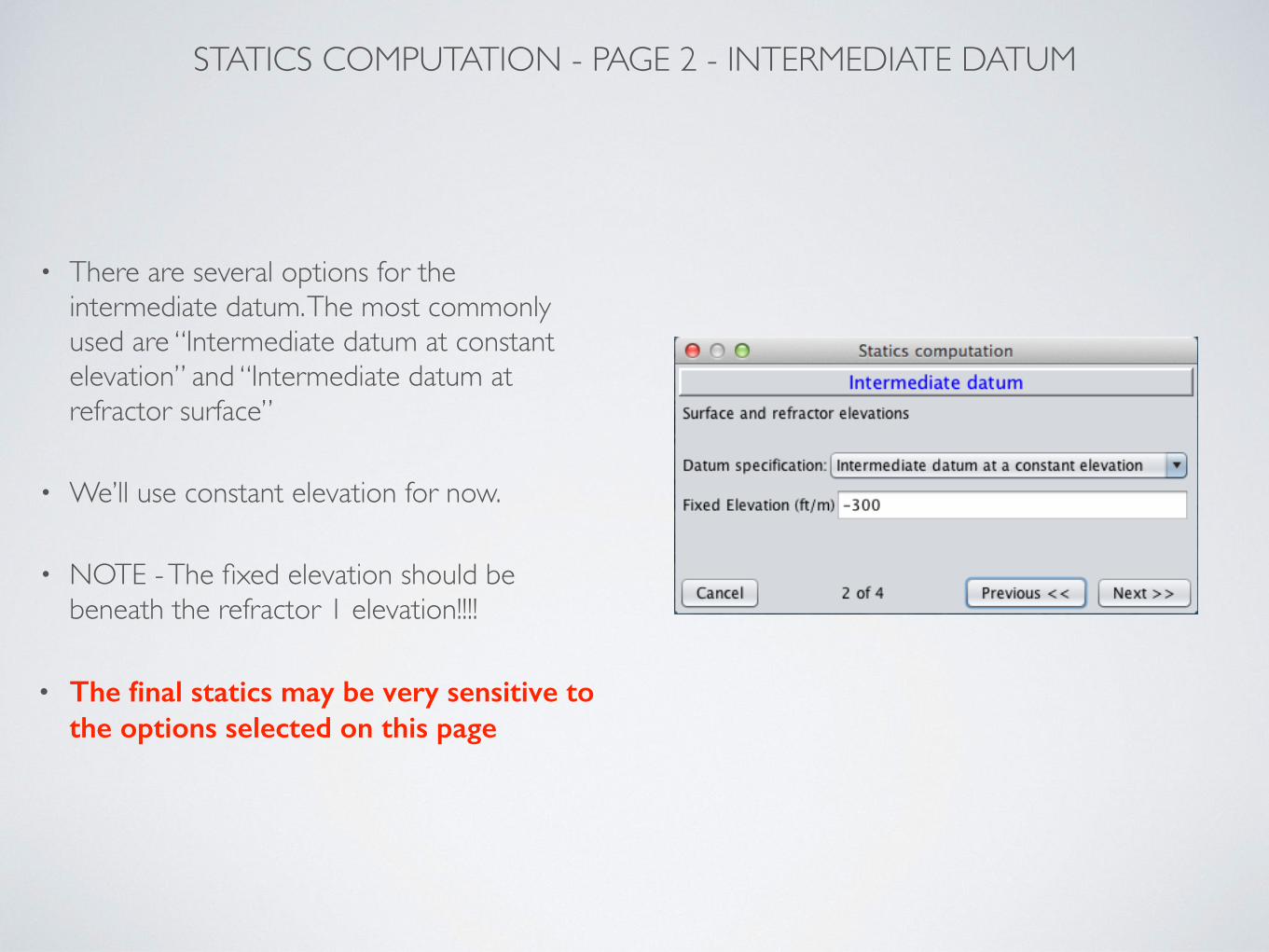
STATICS COMPUTATION - PAGE 2 - INTERMEDIATE DATUM
• There are several options for the intermediate datum. The most commonly used are “Intermediate datum at constant elevation” and “Intermediate datum at refractor surface”
• We’ll use constant elevation for now.
• NOTE - The fixed elevation should be beneath the refractor 1 elevation!!!!
• The final statics may be very sensitive to the options selected on this page
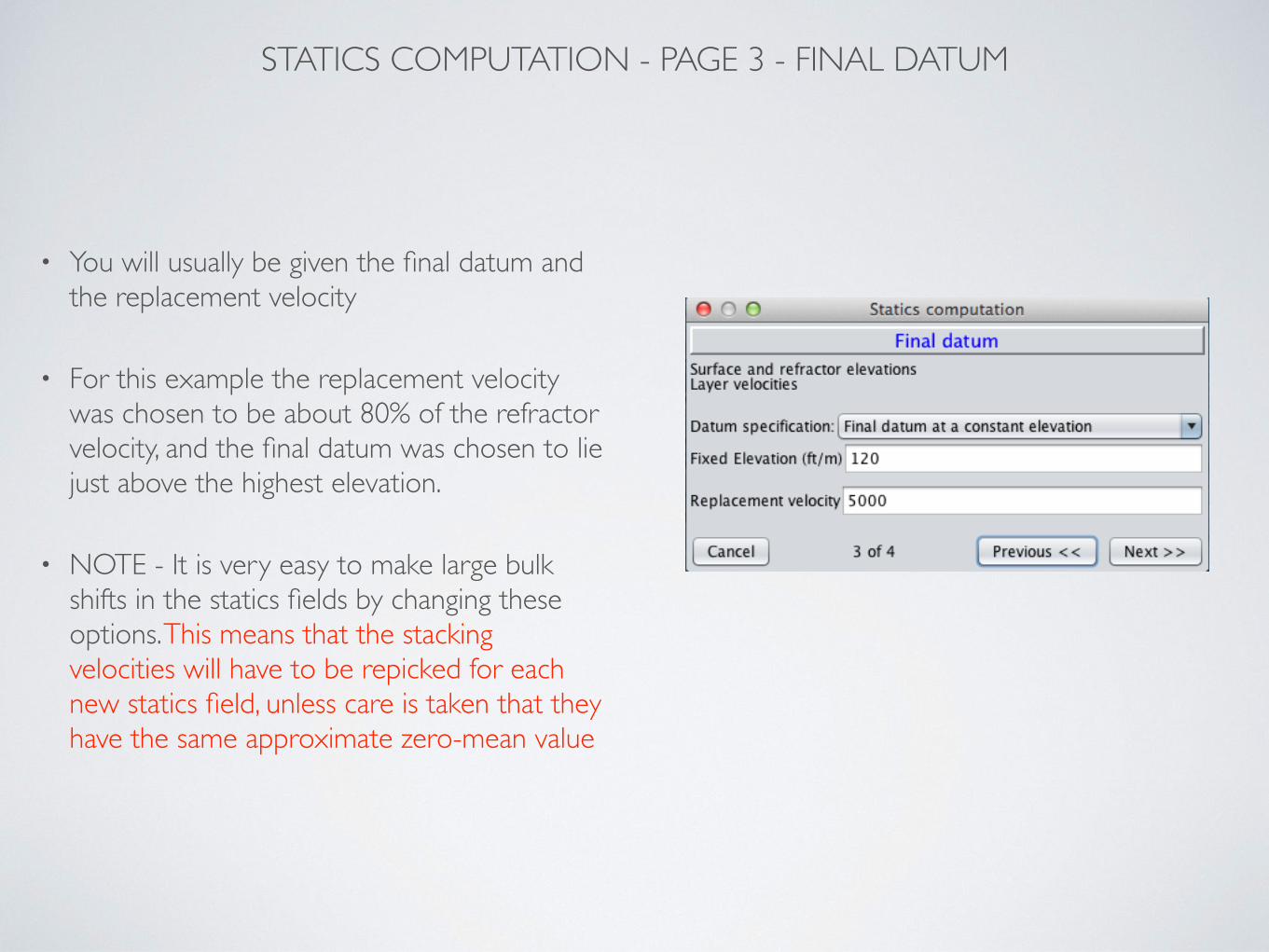
STATICS COMPUTATION - PAGE 3 - FINAL DATUM
• You will usually be given the final datum and the replacement velocity
• For this example the replacement velocity was chosen to be about 80% of the refractor velocity, and the final datum was chosen to lie just above the highest elevation.
• NOTE - It is very easy to make large bulk shifts in the statics fields by changing these options. This means that the stacking velocities will have to be repicked for each new statics field, unless care is taken that they have the same approximate zero-mean value
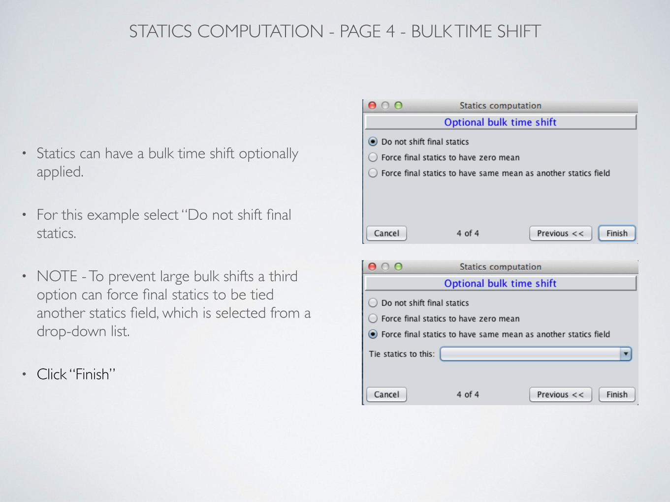
STATICS COMPUTATION - PAGE 4 - BULK TIME SHIFT
• Statics can have a bulk time shift optionally applied.
• For this example select “Do not shift final statics.
• NOTE - To prevent large bulk shifts a third option can force final statics to be tied another statics field, which is selected from a drop-down list.
• Click “Finish”
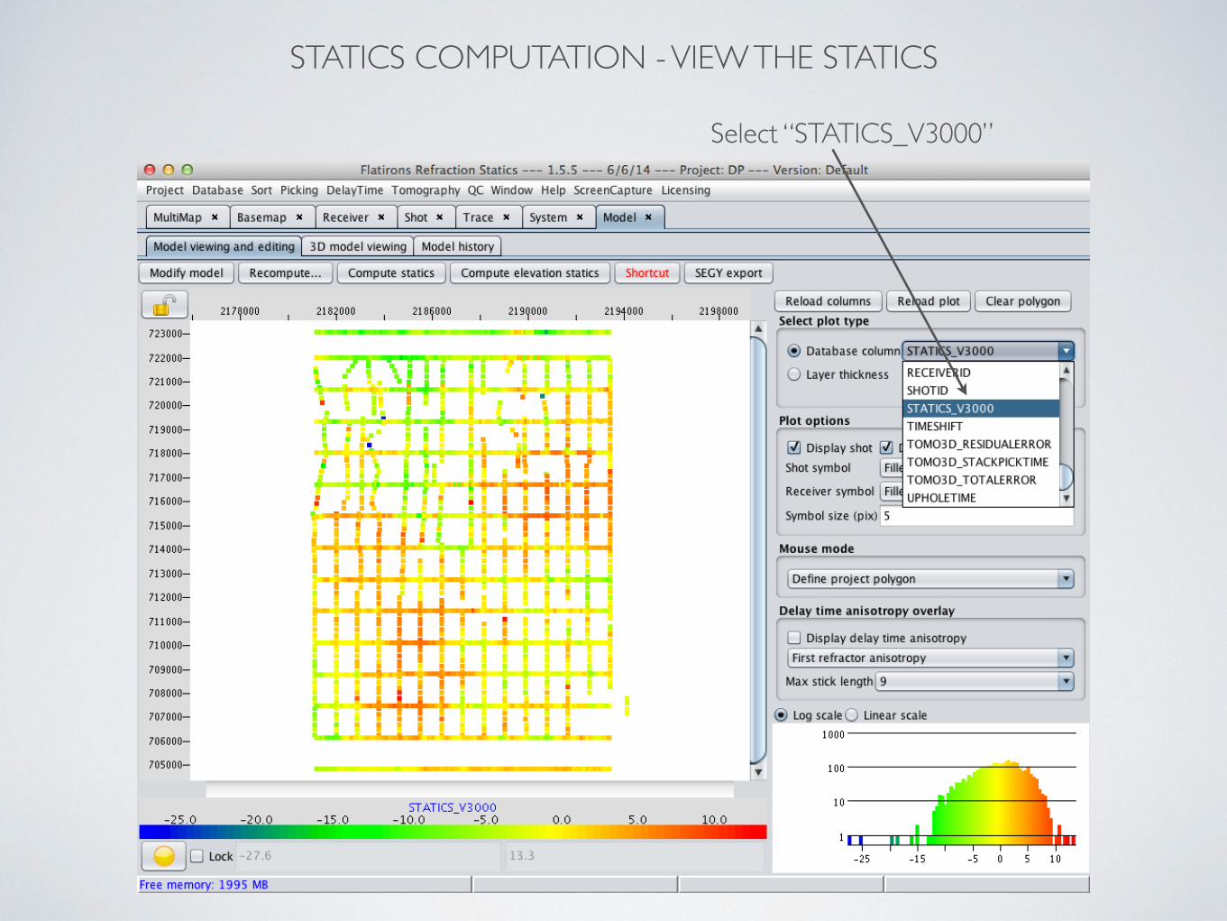
STATICS COMPUTATION - VIEW THE STATICS
Select “STATICS_V3000”
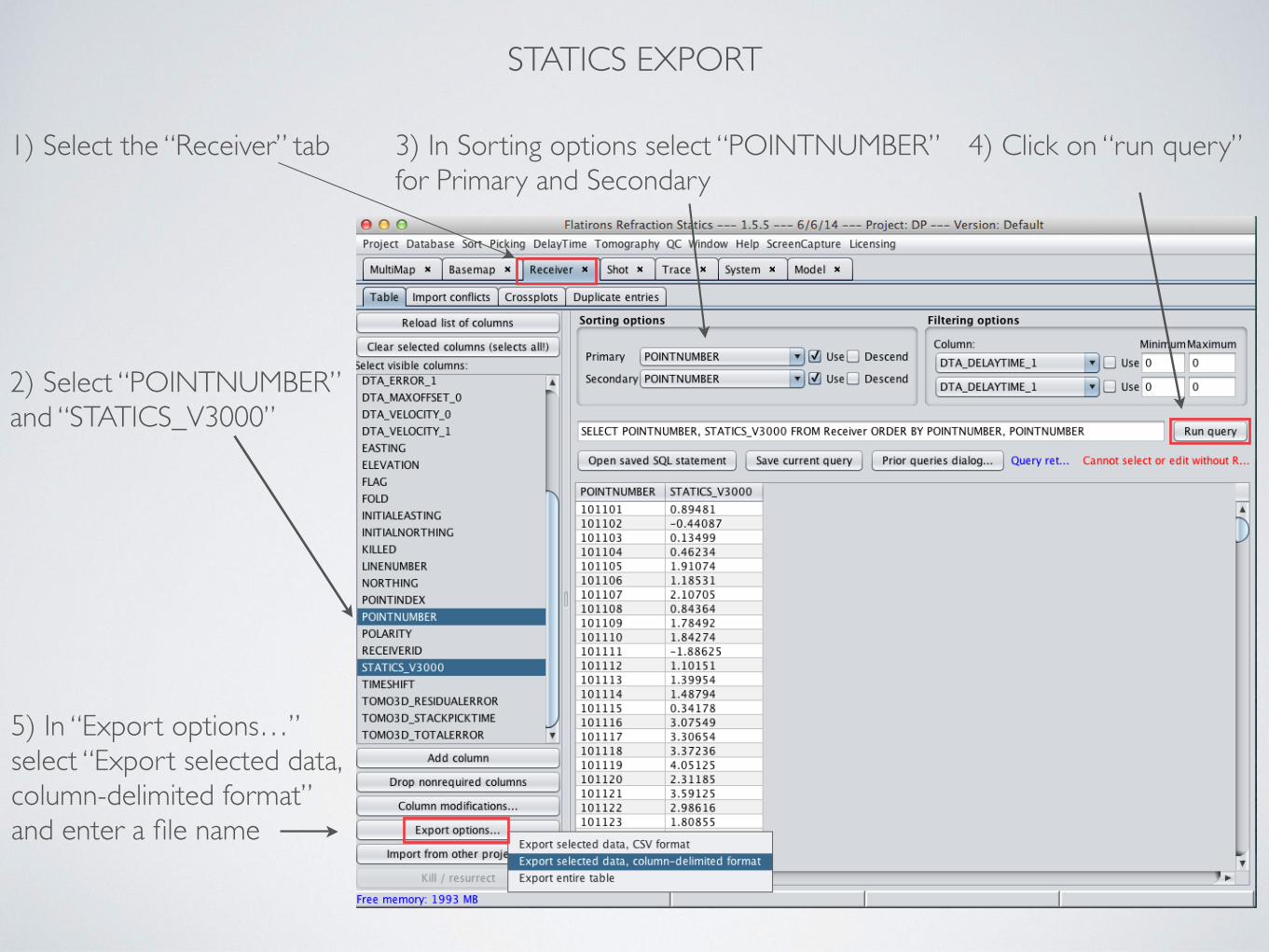
STATICS EXPORT
1) Select the “Receiver” tab
2) Select “POINTNUMBER” and “STATICS_V3000”
3) In Sorting options select “POINTNUMBER” for Primary and Secondary
4) Click on “run query”
5) In “Export options…” select “Export selected data, column-delimited format” and enter a file name

END OF FLATIRONS TUTORIAL - AUTO PICKER © 2014 XtremeGeo Inc.