1

Food for Thought:

The Cognitive Effects of Childhood Malnutrition in the United States

Susan L. Averett (Lafayette College)

and

David C. Stifel (Lafayette College)*

Corresponding author:

David C. Stifel Department of Economics & Business

Lafayette College Easton, PA 18042

e-mail: stifeld@lafayette.edu

Phone: 610-330-5673 Fax: 610-330-5715

* An earlier version of this paper was presented at the 2006 Population Association of America Annual Conference, the 2006 Eastern Economic Association Annual Conference, and the 2006 Economics and Human Biology Annual Conference. The authors would like to thank the participants for their comments.

2

Food for Thought:

The Cognitive Effects of Childhood Malnutrition in the United States

Abstract:

The U.S. faces two types of childhood malnutrition – the prevalence of overweight children

has increased dramatically over the past two decades and the degree of underweight has been

unacceptably high. Both forms of malnutrition create public health problems. Less is known

about how childhood over- or underweight affects a child’s cognitive functioning. We use

data from the children of the NLSY79 to investigate the cognitive consequences of child

malnutrition. We use several estimation methods to control for various forms of endogeneity.

Our results suggest that malnourished children tend have lower cognitive abilities when

compared to well-nourished children.

3

INTRODUCTION

Health is an important dimension of well-being. Not only is it instrumentally

significant through its effects on individual productive capacity and income-earning abilities,

but it is also “intrinsically” significant as it affects individuals’ capabilities to function in

society (Dreze and Sen 1989; Sen 1985, 1987, 1999). Further, as nutrition is an important

element of health, nutritional deprivations can have adverse effects on well-being. In light of

this, this paper addresses one avenue through which malnutrition can affect capabilities, that

is through its effect on cognitive development. In particular, we examine the effect of

childhood undernutrition and overnutrition on test scores in the United States.

The United States is currently characterized by the coexistence of two forms of

childhood malnutrition. On the one hand, the prevalence of overweight children has increased

dramatically over the past two decades1 (Hedley et al. 2004). On the other hand, the degree of

underweight among children has been unacceptably high for such a wealthy country

(Polhamus et al. 2003). Both forms of malnutrition create public health problems. For

example, an overweight child is more likely to be obese as an adult and has a higher

probability of suffering from Type 2-diabetes, high cholesterol, high blood pressure, some

types of cancer, and heart disease than is a child who is not overweight (Dietz 1998;

Schwimmer et al. 2003). Furthermore, the Surgeon General has linked childhood overweight

to social discrimination and depression (U.S. Office of the Surgeon General 2001). At the

other end of the weight distribution, children who do not get enough to eat are likely to suffer

from stunted growth and hindered mental development (Center on Hunger and Poverty 1998).

Paradoxically, although stunted growth (low height-for-age) and wasting (low weight-for-

1 The term overweight is commonly used to refer to obese children as it is less stigmatizing

4

height) are more prevalent in poor families (Miller and Korenman 1994), many poor children

today are overweight. This has led some researchers to describe the problem as one of

“misnourishment,” where instead of getting the necessary healthy food that their bodies need,

children take in excessive amounts of inexpensive fats and calories (Bhattacharya and Currie

2001). The strain that these consequences of child malnutrition will place on the health-care

system are worthy of investigation.

Although the adverse effects of undernutrition on the cognitive functioning of children

are well documented in the United States and around the world (Alaimo et al. 2001; Brown

and Pollitt 1996; Center for Hunger and Poverty 1998; Gardner and Halweil 2000a and

2000b; Pollitt et al. 1996; and Reid 2000), less is known about the effects of obesity.

Although it is indirect, there is some evidence from the medical literature that obese children

may suffer cognitive deficits. This follows from deficiencies of certain micronutrients such as

zinc, iron and iodine (Taras 2005) for which overweight children are at risk (Nead, et al.

2004). This is exacerbated by changes in food technologies and lifestyles in the United

States, and surprisingly throughout much of the developing world, which have resulted in

what is referred to as the “nutrition transition” (Popkin et al. 2001). This is the process

through which the households have access to, and consume more foods that are not only

cheap, energy-rich and convenient, but which are also nutrient-poor. The result of this is

increasing rates of obesity and micronutrient deficiencies among children.

In this research, we use data from the children of the National Longitudinal Survey of

Youth 1979 cohort (NLSY79) to investigate this potential cognitive consequence of childhood

malnutrition. For example, in addition to stunted growth, underweight children are also more

likely to experience emotional, academic and behavioral problems than are well-nourished

5

children (Center on Hunger and Poverty 1998; Jyoti et al. 2005; Kleinman et al. 1998).

Furthermore, overweight children may suffer taunting from their peers resulting in low self-

esteem, low academic achievement and even behavior problems. Thus concerns over the cost

of health care are not the only concerns that policy makers should have as they study the

misnourishment of children. Because of the potential link to cognitive development, there are

legitimate concerns over the future economic effects of malnutrition-induced diminished

productivity (Owens, 1989). These have motivated advocates to emphasize the public

financial costs of malnutrition (obesity in particular) as a strategy to encourage policy makers

to address the issue. The role for public policy follows from the externalities associated with

malnutrition. As Paul Krugman (2005) succinctly describes it, “many of these costs fall on

taxpayers and on the general insurance-buying public, rather than on the obese individuals

themselves.”

However, in our analysis, we aim to discover whether there are additional private

costs such as stunted cognitive development. These costs may manifest themselves in the

future if children who are currently malnourished are likely to be less productive members of

society. For example, researchers have established that obese adults earn lower wages (e.g.

Averett and Korenman 1996; Cawley, 2004). The importance of highlighting these private

costs is that the primary decision makers for children vis-à-vis food consumption and exercise

are parents. Thus, the results from our study may well influence the thinking of parents as

they become aware of the possibility that, in addition to healthcare issues, their children’s

future earning potential may be threatened by their current nutritional status. Further, as these

important private costs also translate into social costs such as lower labor market productivity,

policy makers will also consider them in addition to the healthcare costs.

6

Our research on the effects of childhood malnutrition on cognitive ability improves on

past research in several ways. First, many previous researchers did not use nationally

representative samples, thus limiting the degree to which their results can be generalized.

Second, previous researchers often focused on either underweight or overweight rather than

both extremes of the distribution. Third, we also examine the depth of malnutrition—for

example we find that overweight children are heavier than those children who were

overweight 20 years ago. Fourth, we explicitly recognize the potential for at least two sources

of endogeneity and we take steps to tackle them. To address reverse causality, we use the

method of instrumental variables. To the extent that our instruments are valid, the IV models

allow us to obtain causal estimates of the effect of childhood malnutrition on the outcomes we

study. This is important because those children who have poor cognitive functioning may

over or under eat to compensate for that, thus suggesting the possibility of reverse causality.

We also address time invariant unobserved heterogeneity by estimating individual fixed

effects models.

The remainder of this paper is organized as follows. We begin by describing our data

in section 2. We then provide some background on measurement and trends in child

malnutrition in the United States in section 3, before examining the relationship between child

malnutrition and cognitive ability and behavior as described in our data and in the literature

(section 4). In section 5, we outline the theoretical foundations of our estimation strategy, and

use a brief review of the literature on overweight children to motivate our choice of

explanatory variables and instruments. Following a discussion of the results in section 6, we

close with some concluding remarks.

7

DATA

To investigate the cognitive effects of malnutrition in children, we use data from the

NLSY79, a panel study of approximately 12,000 individuals who were first interviewed in

1979 when they were between the ages of 14 and 22. The female respondents were re-

interviewed annually from 1979-92 and bi-ennially since 1994. The data are a nationally

representative sample of individuals born between 1957 and 1964 with an oversampling of the

black, Hispanic, and low income white populations. Because of this, sampling weights are

used when estimating summary statistics. The data include information about economic and

demographic behavior and outcomes for the respondents and their families.

Our analysis focuses on the children of the original NLSY79 female respondents and

includes data through the 2002 survey year (the latest available to us). At this point, the

mothers are between the ages of 37 and 45 and the children range in age from 3 to 15. It is

worth noting that the sample of children in the NLSY79 is born disproportionately to younger

mothers. This is potentially troubling because these women tend to have lower education and

income levels. However, a great deal of information is available about the family

circumstances of these children over time (e.g., prenatal care and birthweight, family income,

household composition, family structure, and family background). As children who are older

than 13 years of age are likely to have more control over their own food choices, we limit our

sample to elementary school-age children (i.e. ages 6 to 13 years).

Anthropometric measures of height and weight were recorded biennially for each child

beginning in 1986. For approximately 20 percent of the cases, these are reported by the

child’s mother, not measured. They are therefore likely to suffer from measurement error

which may in turn bias our coefficient estimates. Following a thorough cleaning of the data,

8

we address this potential reporting bias by using Cawley and Burkhauser’s (2006) proposed

method of predicting heights and weights based on models estimated from the National

Health and Nutrition Examination Survey (NHANES III).

The NLSY79 data are ideally suited for this analysis because various developmental

measures are available for the children.2 These child assessments have been administered bi-

ennially since 1986 (Baker and Mott 1989; Chase-Lansdale et al. 1991). Thus we have bi-

annual data on children from 1986 to 2002. Our measures of cognitive development are the

math and reading recognition scores from the Peabody Individual Achievement Tests (PIAT)

(Dunn and Barkwardt Jr. 1970), administered to children ages 5 and over. The PIAT is

among the most widely used brief assessments of academic achievement and is an

individually administered measure of academic achievement. The test can be used with

students in kindergarten through the twelfth grade. The PIAT Mathematics assessment begins

with early skills (recognizing numerals) and progresses to measuring more advanced

concepts. The Reading Recognition assessment measures word recognition and pronunciation

ability, which are considered essential components of reading achievement. For both of these

tests, we use the standardized score which has a mean of 100 and a standard deviation of 15.

Reliability of these tests is quite high. Test-retest reliability for the Reading Recognition test

is 0.89 for children from kindergarten through twelfth grade (Baker et al. 1993). The one

month test-retest reliability for the PIAT mathematics assessment is 0.74, with lower levels of

reliability for children in the lower grades (Dunn and Barkwardt Jr. 1970).

2 These data have been used extensively to examine the effect of maternal employment on

cognitive ability (Ruhm 2004) and the effect of paternal child care on children’s cognitive

ability (Averett et al. 2005).

9

MEASUREMENT AND TRENDS OF CHILD MALNUTRITION

A standard for measuring child nutritional outcomes in developed countries is the

Body Mass Index (BMI), which is defined as the ratio of weight in kilograms over height in

meters squared.3 A particular child’s BMI can be compared to those on tables configured by

the Centers for Disease Control (CDC), which established distributions for each sex by age

because BMI levels for children in the healthy reference population differ by age and gender.

A child is considered likely to be overweight if his/her BMI for age is over the 95th percentile

of the healthy reference population,4 while he/she is considered likely to be at risk for

overweight with a BMI for age above the 85th percentile. Children classified as likely to be

underweight are those with BMI for age measures less than the fifth percentile of the

3 Other metrics include stature for age and weight for age for all children (see CDC 2000;

and Martorell and Habicht 1986), and overall evaluation of child health by physicians for

very young children (Wolfe and Sears 1997). While stature for age is a commonly used

measure of chronic malnutrition in developing countries, we do not use it in our analysis as

we consider children up to the age of 15. Martorell and Habicht (1986) find that less than

10 percent of the worldwide variance in height can be ascribed to genetic or racial

differences among children under the age of five. Genetic factors play a much larger role at

older ages and as such, stature for age is not an appropriate measure in our analysis given

our sample of children (described in more detail below).

4 The reference population is based on a sample of healthy children in 2000. See CDC (2000)

for a complete discussion of the reference population.

10

reference population (CDC 2000). In the population, prevalence rates for overweight, at risk

of overweight, and underweight are calculated using these criteria.

To compare BMI measurements across age and gender cohorts, normalized BMI z-

scores (hereafter BMIZ) are calculated. The BMIZ for child i is defined as follows:

BMIZi = refBMI

refBMIiBMI

σµ−

where BMIi is the child’s BMI measurement, refBMIµ is the mean BMI measurement for the

healthy reference population of the same age and gender, and refBMIσ is the standard deviation

of BMI measurements for the healthy reference population of the same age and gender. Since

the healthy reference population is distributed normally, the BMIZ for the reference

population has a standard normal distribution (CDC 2000). Thus, there is a probability

distribution on the expected value of a BMIZ for any given child – a standard normal

distribution to be precise. This means that there is a five percent probability that a child from

the healthy reference population will have a BMIZ greater than 1.645. In other words, 1.645

is the BMIZ cutoff for the 95th percentile (overweight) in the distribution of BMI for age in

the reference population. Similarly, the cutoffs for the fifth (underweight) and the 85th (at risk

of overweight) percentiles are -1.645 and 1.0365, respectively.

To illustrate, in Figure 1 we plot the 1986, 1996 and 2002 distributions of the

normalized BMI for age measures for children in the NLSY79 dataset, along with a standard

normal distribution that represents the reference population. The apparent deviations of the

sample distributions from the reference distribution indicate malnutrition (or

“misnourishment”) among the children in the survey.

11

To make this point clearer, this figure illustrates that the prevalence of overweight

children in this sample rose from 6.7 percent to 18.2 percent between 1986 and 2002 (as seen

by the intersections of the distributions and the overweight cutoff).5 Further it shows that the

prevalence of underweight children remained relatively constant from 1986 to 1996 percent

but fell from 7.2 percent to 4.5 percent from 1996 to 2002.6 With regard to overweight

children, the figure also highlights a weakness of prevalence measures. Not only has the

share of children who are overweight increased, but the degree to which these children are

overweight has increased substantively (as seen by the 2002 distribution being considerably

lower than the 1986 distribution and the reference distribution in the region to the right of the

overweight cutoff).

Discrete measures of over- or undernutrition such as prevalence rates are important for

information-dissemination purposes as they are something that the general public can easily

comprehend. However, focusing only on specific cutoffs such as being above the 95th

percentile or below the fifth percentile can be misleading for two reasons. First, it puts undue

5 More accurately, the prevalence rates should be recorded as 2.8 in 1986, and 17.7 in 2002,

as this represents the difference between the reference distribution and the sample

distributions (i.e. 1.7 = 6.7 – 5.0, and 12.8 = 18.2 – 5.0, respectively). Nonetheless, we

report prevalence rates for all those beyond the threshold as this is the standard practice.

6 These estimates are potentially biased because the age distribution in the 2002 sample is

weighted toward older children relative to the 1986 sample. The implication of this is that

the BMI z-scores of the children at the upper tail of the 1996 distribution are likely to be

biased downward, as are the prevalence rates for 2002 compared to 1986. These potential

biases reinforce our concerns about child malnutrition trends.

12

emphasis on the admittedly arbitrary cutoff points. Marginal changes in the cutoff point can

lead to categorical changes in the recorded health status of a child whose BMI for age

measure is near the cutoff. Second, it ignores the distribution of BMI around the cutoff points.

Thus, in our research, we borrow from the poverty literature by estimating not only

prevalence rates, but also measures of the depth and severity of malnutrition (for overweight,

see Jolliffe 2004; and for underweight, see Sahn and Stifel 2002).

The measures of the prevalence, depth and severity of malnutrition belong to a class of

malnutrition measures that we refer to as Mα. These are defined as follows for underweight:

Mα = ∑=

<−N

iiiN cutBMIZBMIZcut

1

1 )(1)( α ,

and as

Mα = ∑=

>−N

iiiN cutBMIZcutBMIZ

1

1 )(1)( α ,

for overweight, where cut is the under- or overweight threshold, and 1(.) is an indicator

function that takes on a value of one when its argument is true, and zero otherwise. The

parameter, α, can be interpreted as a malnutrition aversion parameter, similar to the poverty

aversion parameter in the Foster-Greer-Thorbecke class of poverty measures (Foster et al.

1984). When α is zero, M0 is the prevalence of malnutrition. When α is one, M1 is the

average malnutrition gap, where a child’s gap takes on a value of zero if he or she is not

malnourished. We refer to this measure as the depth of malnutrition. M2 can be interpreted as

the severity of malnutrition as it is a weighted average of the malnutrition gaps where the

weights are the gaps themselves. The prevalence of malnutrition (M0) is related to the number

of malnourished. The depth of malnutrition considers the distance that the malnourished

children are from the threshold, but weights each child equally. The severity puts more

13

weight on those who are furthest away from the threshold. As α approaches infinity, the

social welfare function associated with the malnutrition measure is Rawlsian. In this extreme

case, when comparing two distributions, the distribution with the most malnourished child is

considered to have more malnutrition. In this paper, we restrict our analysis to the prevalence

(M0) and the depth (M1) of malnutrition.

In Table 1, we present these types of malnutrition metrics applied to the NLSY79 data.

Although underweight is typically thought of as a phenomenon only afflicting developing

countries, it clearly occurs in the United States too. Indeed, we estimate about 6.6 percent of

children between the ages of six and 13 in our sample had BMI levels that fell below the fifth

percentile cutoff in 1986, though this proportion decreased markedly by 2002.7 The

prevalence and depth of underweight children did not change substantially over the decade

from 1986 to 1996. This can also be seen in the form of the stable lower tails of the BMI for

age distributions that appear in Figure 1.

These estimates of undernutrition outcomes are paralleled in the literature on input

measures such as “food insecurity” and hunger. For example, according to the United States

Department of Agriculture (USDA 2004), in 1999, 14 million children lived in “food insecure

households,” which means that their families lacked access to enough food to meet their basic

steady state needs (Center on Hunger and Poverty 1999). Another recent survey estimated

that approximately 4 million American children experienced prolonged periods of food

insufficiency and hunger each year. This is roughly 8 percent of all the children under the

age of 12 living in the United States. The same study shows that an additional 10 million

7 This is consistent with Grigsby’s (2003) estimate of an incidence rate less than 10 percent,

though her estimate is a measure of protein-energy malnutrition (PEM), not underweight.

14

children are at risk for hunger (Kleinman et al. 1998). Finally, in a state by state analysis of

food insecurity in the U.S., Nord et al. (1999) estimate that 9.7 percent of all households were

food insecure during the years 1996-1998.

Not surprisingly, food insecurity is most prevalent in poor families. The Center for

Hunger and Poverty estimates that 35.4 percent of families below the poverty line are food

insecure compared to only 10.2 percent of households nationwide. Paradoxically, however,

children who live in poverty can also be overweight – perhaps because they lack access to

healthy, nutritious low-fat foods (Center for Hunger and Poverty 1999) – which adds to the

confusion over the causes of under- and overnutrition.

Part of this paradox apparently stems from changes in food technologies and prices.

As fast foods become more easily available and as the prices of high-calorie “junk” foods fall

more quickly than the prices of fresh fruits and vegetables, the poor may stretch their limited

budgets by substituting out of the latter into the former (Bhattacharya et al. 2004; Kennedy

and Goldberg 1995). Bhattacharya and Currie (2001) found that in their sample of food-

insecure youths nearly 20 percent were overweight, with almost one-third consuming excess

amounts of sweets. Even adolescents who are not “food insecure” are likely to be

malnourished – a concept Bhattacharya and Currie (2001) refer to as “misnourishment.”

Indeed, the determinants of food insecurity and malnutrition outcomes (underweight and

overweight) are quite different. It is because of this difference and the apparent poverty-

obesity “paradox” that Bhattacharya et al. (2004) conclude that, controlling for poverty, food

insecurity is simply not a good predictor of poorer nutrition outcomes.

15

As indicated in Table 1 and in Figure 1, the prevalence of underweight among children

in the United States has remained stable until recently when it fell.8 The same, however,

cannot be said for the prevalence and degree of overweight children. Using the NLSY79 data,

we find that the share of children who are overweight rose by nearly 6.1 percentage points

between 1986 and 1996, and by an additional 5.4 percentage points between 1996 and 2002.

Further, the depth of overweight rose from an average of 0.03 standard deviations above the

cutoff in 1986 to 0.53 standard deviations in 2002. In other words, not only is there a larger

share of children who are considered to be overweight, the degree to which they are heavier

has grown substantially.

This rapid rise in overweight children has been particularly pronounced over the past

25 years. A Department of Health and Human Resources report (2002), estimates that for a

similar age group (6 to 19), 15 percent (almost 9 million) were overweight in 1999-2000.

This is triple the rate in 1980. Among a younger cohort of children between the ages of two

and five, over 10 percent are overweight, representing a 7 percent increase from 1994 (Ogden

et al. 2002).

8 Note that although the percentage of children with low weight is no more than we would

expect to see in the healthy reference population, the degree to which these weights are low is

higher than expected (e.g. the average underweight gap in the sample is 3.3 standard

deviations, compared to 2.1 standard deviations for the reference population).

16

CHILD MALNUTRITION AND COGNITIVE DEVELOPMENT

One often-cited concern about undernutrition in children is that it may have negative

consequences for cognitive development presumably because a lack of food deprives the

brain of essential nutrients. Although this is generally an issue in the developing world, there

is also a fairly sizeable literature on this topic in the medical field for the United States.

Corman and Chaikind (1998), for example, find that low-birthweight children score lower on

tests of academic performance. Alaimo et al. (2001) report that children aged 6 to 11 in food-

insecure households scored lower on arithmetic tests, were more likely to have repeated a

grade and to have seen a psychologist, and had difficulty getting along with other children.

Winicki and Jemison (2003) also find that food insecurity negatively impacts the academic

performance of kindergartners. Recent research provides compelling evidence that

undernutrition can have detrimental effects on the cognitive development of children and on

their behavior and that this may even impact their later adult productivity (Center On Hunger

1998). Weinreib et al. (2002) report that severe child hunger is correlated with a greater

incidence of behavior problems and is also correlated with a greater level of reported

anxiety/depression. There is evidence that programs such as providing breakfast to school age

children have been effective in mitigating these consequences (Murphy et al. 1998). This has

become such a strongly held view that some schools purportedly manipulated the nutritional

content of their lunches to improve their test scores (Figlio and Winicki 2002).

At the other end of the weight distribution, there are concerns that overweight children

may also suffer from nutrient deficiency (Nead et al. 2004), as well as low self-esteem and

that low self-esteem may lead to lower academic performance or a perceived inability to

perform well in school (Davison and Burch 2001). For adults, it has been demonstrated that

17

obese women have lower self-esteem than their non-obese counterparts (Averett and

Korenman 1999, 1996). This also appears to be the case for children (Eisenberg et al. 2003),

with the effect increasing with age (Strauss 2000). Furthermore, overweight children are more

likely to be more socially isolated compared to adolescents who are not overweight (Strauss

and Pollack 2003). There is also evidence that overweight children have lower academic

performance (Datar et al. 2004), and are more likely to have behavior problems (Datar and

Sturm 2004), to act as bullies, and to be bullied (Janssen et al. 2004). The social functioning

of overweight children is likely to be reduced so much that Schwimmer et al. (2003) compare

their qualities of life to those of children with cancer.

Basic evidence from the NLSY79 data is generally consistent with the literature. As

illustrated in Table 2, children who are categorized as obese according to their BMI tend to

fare worse vis-à-vis test score outcomes.

As the figures in Table 2 are only for a select number of years, we also plot the

evolution of the PIAT math and reading recognition scores by nutritional status for each of the

survey years (Figures 2 and 3). The patterns that emerge in these three figures are striking.

Cognitive ability improves over time for all nutrition groups. However, there remain distinct

differences in these scores at any point in time with healthy kids generally having higher

cognitive scores than malnourished children. It is interesting to see that in the past two years,

PIAT math scores have been greater on average for those children considered at risk of

obesity. This may reflect the fact that there are so many more children in this category over

time. The general story, however, is that although test scores have improved among

malnourished children in the NLSY79 sample, they remain at a disadvantage relative to

healthy children.

18

THEORY AND ESTIMATION STRATEGY

The theoretical foundations for modeling cognitive ability are based on integrating

health and cognitive ability production functions into a common-preference model of

household decision-making in the tradition of Becker (1981).

We start with the assumption that all household members have the same preferences.

As such, the household can be treated as a single individual who maximizes a quasi-concave

utility function that takes as its arguments the consumption of commodities and services, q,

leisure, l, health status, H (of which, a child’s anthropometric measurement, n, is one

dimension), and cognitive ability, C, of each household member. Without considering the

precise household decision-making process, though recognizing that parents make

consumption decisions for young children, the household solves the following problem,

ywTTTlwpqts

XCHlqu

CH

CHlq

+≤+++ )(..

);,,,(max,,,

(1)

where X represents individual, household and community characteristics, some of which are

not observed. Allocation choices are made conditional on the full-income budget constraint,

where p is a vector of prices, w is a vector of household members’ wages, T is a vector of the

household members’ maximum number of work hours, y is sum of all household members’

non-wage income, and TH and TC are time inputs into the production of health and cognitive

ability.

The nutritional status of children, n, is determined by a biological health production

technology:

),;( inni XInn µ= , (2)

19

where In is a vector of health inputs, and iµ represents the unobservable individual, family,

and community characteristics that affect the child’s nutritional outcomes. Specific household

and community characteristics (e.g., demographics, educational levels, etc.), Xn, can have an

impact on health by affecting household allocation decisions.

Similarly, the cognitive abilities of children, c, are determined by cognitive production

technologies:

),;,( iciCi vXnIcc = (3)

where Ic is a vector of cognitive inputs, and vi represents the unobservable individual, family,

and community characteristics that affect the child’s cognitive ability. These production

technologies differ, however, in that the child’s nutritional status, n, is also an input into the

production of cognitive ability.

Ideally, we would estimate these production functions. However, the input vectors, I,

include consumption goods, q, which contribute positively to household welfare both directly

through q, and indirectly through H and C. They also include time inputs, TH and TC, which

are choice variables that affect labor earnings and consumption of leisure. As such, the choice

of consumption goods and health/cognitive inputs is simultaneous and makes consistent

estimation of the production functions impossible in the absence of valid instruments for all of

the inputs. Instead, by solving the household’s optimization problem, we obtain reduced-form

demand functions. For child nutritional status, this can be represented as follows:

),,,,(~),),,,,(( inninnni ywpXnXywpXInn εε == , (4)

where iε is the child-specific random disturbance term, which is assumed to be uncorrelated

with the other elements of the demand function.

20

For cognitive ability, if we note that inputs and nutritional status are functions of

exogenous information,

),),,,,,(~),,,,(( icinncci XywpXnywpXIcc ξε= ,

then a quasi-reduced form demand function can be estimated,

),,,,),,,,,(~(~iccinni ywpXywpXncc ξε= , (5)

where iξ is the child-specific random disturbance term, which is also assumed to be

uncorrelated with the other elements of the demand function. This is a quasi-reduced form

demand function because it is a function of nutritional status, which is represented here by the

reduced form function of exogenous information. Note that identification of the effect of

contemporaneous nutritional status, n, on cognitive ability, c, requires differences in

functional forms, or that the exogenous characteristics and prices that determine nutritional

status, Xn and pn, differ from those exogenous characteristics and prices that determine

cognitive ability, Xc and pc, respectively.

The basis of our estimation strategy can thus be summarized by the following

equation:

cit = α + Xit’β + nit’γ + wt’ δ+ pt

’η + εit (6)

where cit is a measure of cognitive ability for child i at time t,, Xit is a vector of individual-

level, family-level and community-level observables, and nit is a vector of measures of

nutritional status (allowing for malnutrition) for child i at time t. The vector of parameters of

interest is γ. To allow for differing types of malnutrition (overweight and underweight) to

affect cognitive development differently, we estimate three general forms of model (6) in

which nutritional status enters as (a) a set of dummy variables indicating underweight or

overweight, (b) a BMIZ quadratic, and (c) BMIZ along with the malnutrition gap. We also

21

present models in which BMIZ is entered linearly for comparison purposes.

Ordinary least squares (OLS) estimates of model (6) provide unbiased estimates of γ

only if the child’s nutritional status is exogenous, that is it is uncorrelated with the error term

(i.e. E(ε|n) = 0), and the direction of causality goes from nutritional status to cognitive

development. If these conditions do not hold, then the OLS estimator will be biased. There

are two general reasons why we might expect such a bias.

First, there may be unobserved characteristics that simultaneously determine cognitive

ability and nutritional status. In such a situation, changes in these unobservable

characteristics lead to coincidental changes in nutrition and cognitive development. The OLS

estimator will be biased here because it attributes this change in cognitive development to the

change in nutritional status. An example of one such unobservable is parental behavior.

Datar et al. (2004) found that overweight kindergartners were more likely to come from poor

families in which the parents did not read to their children or encourage good academic

performance. This makes it difficult to determine if being overweight is truly the cause of the

poor academic performance, or if poor parenting or some other factor is the cause of both the

overweight and the poor academic performance. Davison et al. (2005) report that some

family environments are obesigenic. In these families mothers and fathers have high dietary

intake and low physical activity and the children in these families are at increased risk of

obesity from ages 5 to 7 years. Unobserved school characteristics may also lead to biased

estimates as they may be an important determinant of both academic achievement and

nutritional status (Crosnoe and Mueller, 2004).

Second, the direction of causality may go both ways independently of unobservables.

For example, while being overweight may cause low self-esteem, depression or other adverse

22

health outcomes and consequently low cognitive development, depression (which may stem

from low cognitive ability) may be a cause of obesity (Goodman and Whitaker 2002). In our

view, most of the previous research on children’s weight and academic performance has not

adequately addressed the issue of causality versus correlation. Although clearly not feasible,

the ideal experimental design would be to randomly “assign” children to be overweight,

underweight, or well nourished. If the assignments were truly random and children who were

either over or underweight performed lower on tests of cognitive ability, we could be

confident that it was their nutritional status that caused the relatively poor performance.9

Given that such an experiment is not feasible, we adopt three empirical methods for

dealing with what we perceive to be the two separate and important sources of endogeneity —

unobserved heterogeneity and reverse causality. We begin by estimating OLS models of

equation (1) as a base of reference using as wide an array of control variables as possible to

address potential heterogeneity and to avoid omitted variable bias. Our first method to

address the endogeneity of nutritional status is to employ instrumental variables. This two-

stage least squares (2SLS) method involves estimating a (set of) first stage equation(s),

nit = θ + Xit’φ + Zit’λ + νit (7)

where Z is a set of instrumental variables that are excluded from model (6). The criteria for

suitable instruments are that they are highly correlated with nutritional status but uncorrelated

with the error term in model (6). In other words, the only effect that a suitable instrument

may have on cognitive ability is indirect, through its effect on nutritional status. Values for

9 Interestingly, some experimental studies similar in design to this have been carried out and

have found that students who fasted before school scored lower on tests of cognitive ability

(Pollitt et al. 1998).

23

nutritional status predicted using the parameter estimates from the first stage estimation (7),

itn̂ , are then used as an explanatory variable in model (6) instead of observed nutritional

status, itn ,

Cit = α + Xit’β + itn′ˆ γiv + wt’ δ+ pt

’η + εit (8)

Given appropriate instruments, the IV estimator (γiv) is an unbiased estimate of γ, the

causal effect of nutritional outcomes on cognitive ability. This approach not only addresses

the concern of reverse causality, but also, because the instruments are uncorrelated with the

error term, it removes biases in the estimator due to unobserved heterogeneity. The difficulty,

of course, is finding suitable instruments that explain nutritional outcomes, but not academic

achievement.

The strong genetic component of child weight (Cawley 2004; Grilo and Pogue-Geile

1991; Strunkard et al. 1986; Volger et al. 1995) indicates that a potential instrument is the

mother’s BMI. However, mother’s current BMI is likely correlated with other unobservable

family-level environmental characteristics that affect the child’s cognitive ability.10 To

10 Several other potential instruments were explored, but proved fruitless. For example, as

policymakers have called for schools to require that students spend more time in physical

education (National Association of State Boards of Education 2000; American Academy of

Pediatrics 2003), we merged our data with the School Health Policies and Programs Study

(SHPPS) data from 1994 and 2000 on state-level physical fitness requirements. Our

findings among elementary school children, however, were similar to Cawley et al. (2005)

who found no link between state physical education requirements and the probability that a

given high school student is overweight. Furthermore, state-level school policies on soft-

24

minimize the possibility that mother’s BMI is correlated with the error term in the second

stage, we use an historical measure of mother’s BMI from 1981.11 For nearly all of the cases

in our sample, this BMI measurement was taken before the birth of the mother’s first child,

and as such is more likely to measure the genetic component of child weight than does the

contemporaneous measure of mother’s BMI. Indeed, a simple regression of mother’s

contemporaneous BMI on her 1981 BMI reveals that only 42 percent of the variation in

current BMI is explained by historical levels. Nonetheless, we also include as control

variables proxies for unobserved household environment and mother’s unobserved abilities

and attitudes that may be more/less favorable to cultivating higher academic achievement.

These proxies include a dummy variable indicating if the child was breastfed, average

household income since the child was born, and the mother’s AFQT score and education

level. We note that since these variables are employed as proxies for mother’s attitudes and

drink vending policies available in the SHPPS data lacked the variation necessary to serve

as a valid instrument for child nutritional status. The NLSY79 also has information on the

average time that a child spends watching television. Research by medical doctors generally

shows a negative effect of TV on different measures of academic achievement

(Borzekowski and Robinson 2005; Chernin and Linebarger 2005) but recent research by

economists reports evidence that television has a negligible effect on cognitive ability.

(Gentzkow and Shapiro 2006). Thus, the available evidence suggests that television

watching is not a suitable instrument for us.

11 Genetic variation in weight as measured by parental weight status is also used by an

instrument for child’s BMI by Sabia (2007) in his examination of the effect of adolescent

obesity on GPA.

25

household environment, the parameter estimates for these variables should not be interpreted

as indicating a causal relationship. The parameter estimate for the breastfeeding dummy, for

example, is not expected to represent the true effect of breastfeeding on cognitive ability. We

remind the reader that the object of interest in this analysis is the γ parameters, not the

potentially biased β parameters.

Our second approach to addressing unobserved heterogeneity (but not reverse

causality) is to take advantage of the panel nature of the NLSY data and to estimate individual

fixed effects (FE) models. Thus model (6) becomes

Cit = α + µi + Xit’β + nit’γ + wt’ δ+ pt

’η + εit (9)

where µi is a child-specific dummy variable12, and Xit now includes only those explanatory

variables that are not fixed over time. The effectiveness of the fixed effects estimator in

reducing the bias in γ depends on the unobservable characteristics that affect both nutritional

outcomes and cognitive development being fixed over time and consequently differenced

out.13 Thus, this model improves on OLS but may not be ideal if factors influencing cognitive

12 This is also referred to as the “within” estimator as it is equivalent to estimating a model of

differences in within-individual means.

13 We also estimated sibling fixed effects models, the results of which were qualitatively

similar to the individual fixed effects models presented here. The motivation for this

approach is that differences between siblings remove variance in weight attributable to a

shared family environment. However, Cawley (2004) argues that this is not an appropriate

way to remove unobserved heterogeneity citing evidence that shared family environments

explain a negligible proportion of the variance in weight across siblings. However, others

26

ability and BMIZ vary over time. Further, as noted earlier, FE models do not eliminate the

potential for reverse causality.

In our third approach, we employ an IV method that differs from the standard IV

estimator due to the means through which identification is obtained. In this method proposed

by Lewbel (2004),14 the identification of γ comes from exploiting the heteroskedasticity of the

first-stage equation (BMIZ). To illustrate, begin by defining the first stage equation as

nit = θ + Xit’ς + νit (10)

where X can include all or a subset of the explanatory variables in the main (second stage)

equation (6). If Cov(X,v2) is nonzero (i.e. the data are heteroskedastic), then γ and the other

parameters in the main equation can be estimated consistently without external instruments by

an ordinary linear two stage least squares regression in which all of the exogenous right hand

side variables and ( ) 2v̂XX − are used as instruments for the child’s BMIZ. We estimate

model (6) using this method without external instruments. Breusch and Pagan (1979) tests for

heteroskedasticity are applied to the first stage equations to test the identification requirement

that Cov(X,v2) ≠ 0.

have noted that an obesigenic family environment is an important predictor of children’s

changes in BMI (Davison et al. 2005). We do not report these models.

14 See also Rigobon (2003)

27

RESULTS

Tables 3 through 7 present the results of our estimated models. Table 3 presents the weighted

sample means. Because an important control variable in our model is the mother’s wage, we

predicted mother’s wages for all women in our sample.15 The sample consists of 20,856 child

years. Just under half of the sample is female and the sample of child years is distributed

evenly by age except for the oldest age groups (12 and 13) where there are slightly fewer

child years. Tables 4 through 6 presents the results from OLS, FE and IV estimates of the

determinants of cognitive development as measured by PIAT math and reading recognition

scores. The IV models include the standard 2SLS models (hereafter referred to as IV) and the

models that use heteroskedasticity to identify the parameters of interest (hereafter referred to

as Hetero). The specifications in Table 4 include BMIZ entered linearly and a dummy

variable specification for under and over weight. In table 5, BMIZ is entered as a quadratic,16

while in table 6 we use BMIZ and the overweight gap as our measure of malnutrition. These

tables only include the parameters of interest – the effects of nutritional status – from the

OLS, IV, FE, and Hetero models. Table 7 presents the first stage estimates for the IV models,

15 Predictor variables for this regression were age and education (both measured in years),

their squares and an interaction between them and mother’s AFQT score. Details of this

regression are available upon request from the authors.

16 Because we enter BMIZ nonlinearly (as a quadratic) and since the distribution of z-scores

for a healthy population has a standard normal distribution, we first shift the BMIZ

distribution by 10 points. While this does not change any of the information in the

distribution of BMIZ, it does avoid confusion over how to interpret the squared value of a

negative z-score.

28

while Table 8 presents the parameter estimates for the other control variables in the main

models.

Focusing first on the results for PIAT math scores in Table 4 (top panel), in the OLS

dummy variable specification we find that underweight children score a statistically

significant 1.27 points lower than children whose weight is in the recommended range all else

equal. Given a standard deviation of 15 for this test, the effect is equivalent to scores that are

one eighth of a standard deviation lower. Overweight children do not have significantly

different math scores in the OLS model. Although the pattern of significance is similar, the

coefficients in the FE models are smaller, indicating that there is some unobserved

heterogeneity.

Recall that the OLS and FE models do not account for possible reverse causality.

Hence we turn to the IV and Hetero models. To determine the validity and relevance of our

instruments in the IV model, we report the p-values for the F-test of joint significance of the

excluded instruments (mother’s BMI and BMI squared), and two tests of weak instruments –

the Cragg-Donald statistic17 and the p-value for the Anderson-Rubin test18. Despite the fact

17 This is the multiple equation analog to the F-statistic used in the Stock-Yogo (2005) test,

and is available as an option in Stata’s ivreg2 command. This statistic is used to test if the

instruments are weak. The critical value is the 5 percent value compiled by Stock and

Yogo (2005) and reported by ivreg2. The interpretation is that a Cragg-Donald statistic

above this critical value rejects the null hypothesis that the instruments are weak a the 5

percent level of significance. See also Murray (2005).

18 The Anderson-Rubin F-statistic is used to test the null hypothesis that all of the endogenous

variables are jointly insignificant.

29

that the parameter estimates for the IV models are much larger than for the OLS and FE

models, these test statistics indicate that we can reject the null hypothesis that the instruments

are weak, and that our IV estimates are not much biased. Because our models are just

identified we cannot rely on standard tests of overidentification to determine if the

instruments can be legitimately excluded from model (8). Hence, we focus on the intuition

that there is a strong genetic component to weight as referenced above, and that by using an

historical measure of the mother’s BMI, the instrument should be less correlated with the

child’s current home environment.19 Experiments were conducted using alternative

instruments such as sibling nutritional status and district-level fast-food prices. The results of

these estimates are similar to those presented here and are available upon request from the

authors.

The IV models clearly indicate that children at both ends of the nutrition spectrum —

underweight and overweight — have lower test scores on average. Underweight children have

PIAT math scores that are nearly one and a quarter standard deviations lower than those of

children with BMIZ scores in the recommended range (18.76/15). Overweight kids have

PIAT math scores that are about six-tenths of a standard deviation lower than their well-

nourished peers, all else equal (9.21/15). In the Hetero models, only the effect of overweight

19 As an informal test of the intuition of the instruments, we estimated reduced form

regressions with the instrumental variables as the explanatory variable and test scores as the

dependent variables. The instrumental variables have coefficients that are significantly

different from zero and have signs that support the genetic-component identification story –

positive for mother’s BMI and negative for mother’s squared BMI. (See Murray 2006)

30

is statistically significant, with a magnitude that is similar to the IV model. We reject the null

hypothesis of no heteroskedasticity using a standard Breush-Pagen test.

The bottom panel of table 4, the PIAT reading recognition scores, tells a slightly

different story. In the dummy variable specification using OLS, we see that PIAT reading

scores are significantly lower for overweight children but not for underweight children (the

opposite of the case for the PIAT math scores). This pattern is the same for the FE models

though the coefficient is slightly smaller. The IV and Hetero results are similar across math

and reading scores in that they are much larger than the OLS and FE coefficients, though the

effect of malnutrition on PIAT reading recognition scores in the Hetero models is

considerably smaller than the IV models (0.2 standard deviations lower for the former

compared to 1.5 standard deviations lower for the latter).

Turning to the models in table 5 where BMIZ is entered as a quadratic, a clear pattern

emerges for the PIAT math scores (top panel). The positive and significant coefficients for

BMIZ and negative and significant coefficients for squared BMIZ indicate that as BMIZ

scores rise, PIAT math scores first rise and then fall. This pattern is consistent in sign and

significance across the estimation procedures used. The only difference is that the magnitude

of the coefficient estimates in the OLS and FE models is considerably smaller than for the IV

and Hetero models.

To facilitate interpretation of the non-linear effect of the BMIZ quadratic in table 5,

we calculate marginal effects at points of interest in the BMIZ distribution (i.e. at the

underweight, at-risk of overweight and overweight thresholds) and test if these effects are

significantly different from zero. These marginal effects reveal a consistent statistically

significant effect for children at the underweight threshold. An improvement in nutritional

31

status beyond this threshold improves test scores. For example, a 1 standard deviation

increase in BMI for age at the underweight threshold leads to PIAT math scores increasing

from 0.036 standard deviations in the FE model (0.55/15) to 0.82 standard deviations in the

IV model.20 Although the marginal effects calculated at the at-risk of overweight and

overweight thresholds are not statistically significant for the OLS and FE models (though the

coefficient estimates are), they are for the IV model and for overweight in the Hetero model.

For the IV model, a 1 standard deviation increase in BMIZ leads to between a 0.43 (for at risk

of overweight) and 0.71 (for overweight) standard deviation decline in math scores.

A different pattern exists for the coefficients on BMIZ and BMIZ-squared for PIAT-

reading recognition scores (Table 5, bottom panel). The parameter estimates are statistically

significant with the expected signs for the OLS, IV, and Hetero models, but are not

statistically different from zero for the FE model. As before, the IV coefficients are

considerably larger. The marginal effects, however, are statistically significant in the IV

models only for at-risk of overweight and overweight kids but not for underweight kids.

Because the Breusch-Pagan χ2 test statistic is small, indicating that we cannot reject the null

hypothesis of homoskedasticity, the parameter estimates for the Hetero reading recognition

model are suspect.

As noted in section 3, children who are classified as overweight are heavier than they

were even a decade ago. To understand how the depth of overweight affects test scores, the

20 The marginal effects in Table 5 are interpreted as the average change in test scores for a 1

standard deviation increase in BMIZ. To interpret these effects in terms of test score

standard deviations, one needs to divide the marginal effect by the reference population

standard deviation of the test scores (i.e. by 15).

32

results of estimates in which BMIZ and the overweight gap are used as our regressors are

reported in Table 6.21 In this model, the BMIZ in linear form controls for the nutritional status

of the entire population while inclusion of the overweight gap controls for the depth of

overweight. The BMIZ and the overweight gap parameter estimates in the OLS, IV, and

Hetero models all suggest that overweight children have lower math and reading scores. The

coefficient estimates in the FE models were not statistically significant, and as with the

previous estimates, the null hypothesis of homoskedasticity for the Hetero reading recognition

model is not rejected. In Table 6, we assist the interpretation of parameter estimates on BMIZ

and the overweight gap by simulating the effect of a 0.1 standard deviation increase in BMIZ

on the dependent variables. This is done by applying the parameter estimates to the adjusted

sample distribution of BMIZ, keeping all other factors constant. Note that for children with

BMIZ scores less than 0.1 standard deviations below the 95 percentile threshold initially, their

overweight gaps take on positive values in the simulation. The averages of the resulting

predicted changes in PIAT scores are then reported for all kids and for overweight kids.

Because these are simulations, we do not have tests of significance.22 Our estimates and

simulations reveal a negative effect of being overweight on cognitive ability. The magnitude

of these effects ranges from test scores that are 0.12 to 3.03 standard deviations lower due to a

0.1 standard deviation increase in BMIZ.

The parameter estimates for the other explanatory variables are generally as we might

expect (Table 7). In particular, birth weight exerts a positive and statistically significant

21 We also experimented with using the underweight gap but this was the best fitting model.

22 Test statistics can, however, be formed by bootstrapping these simulations to create

standard errors.

33

effect on cognitive ability. The low birth weight literature generally establishes a strong

negative correlation between birth weight and cognitive ability (Hack et al. 1991; Corman and

Chaikind, 1998; Boardman et al., 2005 and Almond et al., 2002) consistent with our results.

Hispanic children score lower on tests of math than white children, but higher on reading

recognition when compared to white children. Black children score lower on both math and

reading tests when compared to white children. Birth order is an important predictor of

cognitive ability with first born children scoring better on the cognitive tests. Household size

is also an important predictor of cognitive ability with children from larger household having

lower scores on the math and reading recognition tests. Mother’s age is not an important

predictor of a child’s cognitive ability but children with more educated mothers have higher

cognitive ability. Average household income is also an important predictor in the expected

directions. Children in families with more economic resources have higher scores on math

and reading recognition. Again, we caution that strict interpretation of these estimates can be

misleading as they were also included in the models as proxies for unobserved mother’s

behavior and household environment. The urban dummy is not an important predictor of

cognitive ability. Finally, as we saw in the raw data, scores on tests of cognitive ability rise

over time.

Naturally the validity of our IV results depends on how well our instruments perform.

We present the first stage results of our IV estimation in table 7. The mother’s BMI and BMI

squared are significant predictors of a child’s BMIZ score both individually and jointly. The

p-values on the F-statistics testing their joint significance are all less than 1 percent. Further,

the coefficient estimates in the first stage for the IV model are of the expected signs and

magnitudes. Nonetheless, the R-squares in the first stage regressions are low ranging from

34

0.07 to 0.11. Since the magnitude of the bias of the IV estimator is inversely related to the r-

squared from the first stage, the IV estimates in Tables 4, 5 and 6 could be substantively

biased. Indeed it can be shown that when the R-squared from the first stage estimation is low,

even a small correlation between the error and the instrument can lead to a large bias (Murray,

2005). Thus, we cannot rule out that a lack of explanatory power may be causing the IV

estimates to become large. Nonetheless, the large Cragg-Donald statistics and Anderson-

Rubin F-statistics suggest that IV estimation is predictable enough to provide relatively

unbiased parameter estimates (Murray 2006; Stock and Yogo 2005).

To summarize, we find evidence that child malnutrition as measured by BMIZ exerts a

negative effect on cognitive abilities as measured by the PIAT math and reading recognition

scores. In FE specifications using dummy variables to control for malnutrition, we find

evidence that overweight children have lower reading recognition test scores and that

underweight children have lower math scores. The IV models using mother’s historical BMI

as an instrument, and the heteroskedasticity-identification models, suggest a negative effect of

being overweight on both math and reading test scores, and often find a negative effect of

being underweight. While none of these methodologies provides a “silver bullet”, they do

yield qualitatively similar results that collectively provide evidence that deviating from

“normal” weight lowers academic ability as measured by these test scores.

35

CONCLUSION

The prevalence of overweight among children has reached near epidemic proportions

in the United States over the past twenty five years. Our research documents that the

prevalence and depth of childhood overweight has increased over time, and although the

incidence of underweight children has declined, the depth of underweight remains higher than

would be expected in a healthy reference population. Our primary research question is

whether childhood malnutrition, as measured by BMIZ scores, is an important causal

predictor of cognitive ability in elementary school aged children. This is an important

question for parents, school administrators and policymakers. If overweight and/or

underweight children perform poorly on tests of cognitive ability, and if this persists into

adulthood, they are likely to be less productive as adults. This lower productivity has both

private and public costs that arise in addition to the medical costs associated with

malnourishment.

We use data from children born to the women in the NLSY79 to address whether

under- or overweight children have lower cognitive ability. We are particularly interested in

establishing if such malnutrition is a cause of low cognitive ability. Endogeneity, however, is

an important concern with regard to any statistical estimate of this relationship. In particular,

we are concerned about two sources of endogeneity – reverse causality and unobserved

heterogeneity. Therefore, in addition to using standard OLS estimation procedures, we

estimate individual fixed effects models as well as two different types of IV models.

Although standard tests confirm the validity and relevance of our instruments, the explanatory

power of our first stage models is modest.

36

Although there are issues related to each of the estimation methods, the collective

weight of the evidence provided in this analysis suggests that childhood malnutrition (either

underweight or overweight) has a negative effect on cognitive abilities as measured by the

PIAT math and reading recognition scores. Further, we find evidence that the degree to

which a child is overweight matters. While these effects are generally statistically significant,

the range of the magnitude of our coefficient estimates makes it difficult to pin down the

precise impact. Nonetheless, the consistent results of these three estimation procedures

indicates a robustness of our findings. Thus, our research suggests that parents should be

particularly vigilant in monitoring a child’s nutritional status whatever the proximate cause of

under or overweight might be.

37

REFERENCES

Alaimo, Katherine, Christine M. Olson, and Edward A. Frongillo Jr. 2001. “Food

Insufficiency and American School-Aged Children's Cognitive, Academic, and

Psychosocial Development.” Pediatrics 108(1): 44-53

Almond, Douglas, Kenneth Chay, and David Lee. 2004 “The Costs of Low Birthweight.”

NBER Working Paper, No. 10552.

American Academy of Pediatrics. 2003. “Policy Statement: Prevention of Pediatric

Overweight and Obesity .” Pediatrics 112(2): 424-430.

Averett, Susan, and Sanders Korenman. 1996. "The Economic Reality of the Beauty Myth."

Journal of Human Resources 31(2): 304-30.

Averett, Susan, and Sanders Korenman. 1999. "Black-White Differences in Social and

Economic Consequences of Obesity." International Journal of Obesity 23: 166-173.

Averett, Susan, Lisa A. Gennetian and H. Elizabeth Peters. 2005. “Paternal Child Care and

Children's Development.” Journal of Population Economics 18(3): 391-414.

Baker, Paula, K. Keck Canada, Frank L. Mott, and Stephen V. Quinlan. 1993. NLSY Child

Handbook, Revised Edition: A Guide to the 1986-1990 NLSY Child Data. Center for

Human Resources Research. Ohio State University, Columbus.

Baker, Paula, and Frank Mott. 1989. NLSY handbook 1989: A Guide and Resource

Document for the National Longitudinal Survey of Youth 1986 Child Data. Center for

Human Resources Research. Ohio State University, Columbus.

Becker, G.S., 1981, A Treatise on the Family, Cambridge, MA: Harvard University Press.

38

Bhattacharya, Jayanta, Janet Currie and Steven Haider. 2004. "Poverty, Food Insecurity, and

Nutritional Outcomes in Children and Adults.” Journal of Health Economics 23: 839-862.

Bhattacharya, Jay, and Janet Currie. 2001. "Youths at Nutritional Risk: Malnourished or

Misnourished?" In Jonathan Gruber, ed., Risky Behavior Among Youths: An Economic

Analysis, University of Chicago Press for NBER, Chicago.

Boardman, Jason, Robert Hummer, Yolanda Padilla, and Daniel Powers. 2005. “Low Birth

Weight, Social Factors and Developmental Outcomes Among Children in the United

States.” Mimeo.

Borzekowski, Dina L.G. and Thomas N. Robinson. 2005. “The Remote, the Mouse, and the

No. 2 Pencil: The Household Media Environment and Academic Achievement Among

Third Grade Students” Archives of Pediatrics and Adolescent Medicine 159:607-613.

Breusch, T., and Pagan, A. 1979. “A Simple Test for Heteroskedasticity and Random

Coefficient Variation.” Econometrica 47: 1287-1294.

Brown, L., and E. Pollitt. 1996. “Malnutrition, Poverty, and Intellectual Development.”

Scientific American, 274: 38-43.

Cawley, John, and Richard V. Burkhauser. 2006. "Beyond BMI: The Value of More

Accurate Measures of Fatness and Obesity in Social Science Research." NBER Working

Paper No. W12291

Cawley, John. Chad Meyerhoefer and David Newhouse. 2005. “The Impact of State Physical

Education Requirements on Youth Physical Activity and Overweight.” NBER Working

Paper No. 11411

Cawley, John. 2004. "The Impact of Obesity on Wages." Journal of Human Resources 39(2):

451-474.

39

Centers for Disease Control. 2000. Growth Charts.

(http://www.cdc.gov/nchs/about/major/nhanes/growthcharts/clinical_charts.htm)

Center on Hunger and Poverty. 1998. “Statement on the Link Between Nutrition and

Cognitive Development in Children.” (http://www.centeronhunger.org/cognitive.html)

Center on Hunger and Poverty. 1999. “Childhood Hunger, Childhood Obesity-An

Examination of the Paradox.” (http://www.centeronhunger.org/execsums/obesity.html)

Chase-Lansdale, P.L., F. L. Mott, J. Brooks-Gunn, and D. Phillips. 1991. “Children of the

NLSY: A Unique Research Opportunity.” Developmental Psychology 27(6): 918-931.

Chernin, Ariel R. and Deborah L. Linebarger. 2005. “The Relationship Between Children’s

Television Viewing and Academic Performance.” Archives of Pediatrics and Adolescent

Medicine 159:687-689.

Corman, Hope, and Stephen Chaikind. 1998. “The Effect of Low Birthweight on the Health,

Behavior, and School Performance of School-Aged Children.” Economics of Education

Review 17(3): 307-316.

Datar, Ashlesha, and Roland Sturm. 2004. “Childhood Overweight and Parent- and Teacher-

Reported Behavior Problems. Evidence From a Prospective Study of Kindergartners.”

Archives of Pediatrics and Adolescent Medicine (158): 804-810.

Datar, A., R. Sturm, and J.L. Magnabosco. 2004. “Childhood Overweight and Academic

Performance: National Study of Kindergartners and First-Graders.” Obesity Research

12(1): 58-68.

Davison, Kirsten Krahnstoever and Leann Lipps Birch. 2001,. “Weight Status, Parent

Reaction, and Self-Concept in 5 year old girls.” Pediatrics 107(1):46-53

40

Davison, Kirsten Krahnstoever, Lori A. Francis and Leann L. Birch. 2005. “Reexamining

Obesigenic Families: Parent’s Obesity-related Behaviors Predict Girls’ Change in BMI.”

Obesity Research 13: 1980-1990.

Department of Health and Human Services. 2002. Press Release. October 8.

(http://www.os.dhhs.gov/news/press/2002pres/20021008b.html)

Dietz, V.M. 1998. “Health Consequences of Obesity in Youth: Childhood Predictors of Adult

Disease.” Pediatrics 101: 518-525.

Dreze, Jean, and Amartya Sen. 1989. Hunger and Public Action. Oxford: Clarendon Press.

Dunn, L.M. and F. Barkwardt Jr. 1970. Peabody Individual Achievement Test Manual.

American Guidance Service, Inc., Circle Pines, MN.

Eisenberg, Marla E., Dianne Neumark-Sztainer, and Mary Story. 2003. “Associations of

Weight-Based Teasing and Emotional Well-being Among Adolescents.” Archives of

Pediatrics and Adolescent Medicine 157: 733-738.

Figlio, David, and Joshua Winicki. 2002. “Food for Thought: The Effects of School

Accountability Plans on School Nutrition.” NBER Working Paper No. 9319.

Foster, James, Joel Greer, and Erik Thorbecke. 1984. “A Class of Decomposable Poverty

Measures.” Econometrica 52(3): 761-766.

Gardner, Gary and Brian Halweil, March 2000a. “Diet Quality and Health of the Poor.”

Washington, DC: International Food Policy Research Institute.

Gardner, Gary and Brian Halweil, 2000b. “Underfed and Overfed: The Global Epidemic of

Malnutrition.” Worldwatch Paper #150. Washington, DC.

41

Goodman, Elizabeth, and Robert C. Whitaker. 2002. “A Prospective Study of the Role of

Depression in the Development and Persistence of Adolescent Obesity” Pediatrics 110(3):

497-504.

Grigsby, Donna M., M.D. 2003. ”Malnutrition.” eMedicine.

(http://www.emedicine.com/ped/topic1360.htm)

Hack, M, Brellau, N. Weissman, B. Aram D, Klein N, Borawski E. 1991. “Effect of Very

Low Birth Weight and Subnormal Head Size on Cognitive Abilities at School age.” New

England Journal of Medicine 325(4):231-7.

Hedley, Allison A., Cynthia L. Ogden, Clifford L. Johnson, Margaret D. Carroll, Lester R.

Curtin, and Katherine M. Flegal, 2004. “Prevalence of Overweight and Obesity Among

US Children, Adolescents, and Adults, 1999-2002.” Journal of the American Medical

Association 291:2847-2850.

Janssen I., W.M. Craig, W.F. Boyce, and W. Pickett. 2004. “Associations Between

Overweight and Obesity With Bullying Behaviors in School-Aged Children.” Pediatrics

113(5): 1187-1194.

Jolliffe, Dean. 2004. “Continuous and Robust Measures of the Overweight Epidemic: 1971-

2000.” Demography 41(2): 303-314.

Jyoti, Diana, Edward Frongillo and Sonya Jones. 2005. “Feed Insecurity Affects School

Children’s Academic Performance, Weight Gain, and Social Skills.:” Journal of Nutrition

135:2831-2839.

Kennedy, E., and J. Goldberg. 1995. “What are American Children Eating? Implications for

Public Policy.” Nutrition Reviews 53:111-126

42

Kleinman R.E., J.M. Murphy, M. Little, M. Pagano, C.A. Wehler, K. Regal, and M.S.

Jellinek. 1998. “Hunger in Children in the United States: Potential Behavioral and

Emotional Correlates.” Pediatrics 101(1): E3.

Lewbel, Arthur 2004. “Identification of Heteroskedastic Endogenous or Mismeasured

Regressor Models.” Mimeo. Boston College.

Martorell, R., and J., Habicht. 1986. “Growth in Early Childhood in Developing Countries.”

in F., Falkner and J., Tanner, eds., Human growth: A comprehensive treatise, Vol. 3,

Plenum Press, New York.

Miller, Jane E. and Sanders Korenman. 1994. “Poverty and Children's Nutritional Status in

the United States.” American Journal of Epidemiology 140(3): 233-243.

Murphy, J. Michael, Maria E. Pagano, Joan Nachmani, Peter Sperling, Shirley Kane and

Ronald E. Kleinman. 1998. “The Relationship of School Breakfast to Psychosocial and

Academic Functioning Cross-sectional and Longitudinal Observations in an Inner-city

School Sample” Archives of Pediatrics and Adolescent Medicine 152: 899-907.

Murray, Michael P. 2006. “Avoiding Invalid Instruments and Coping with Weak

Instruments.” Journal of Economic Perspectives 20(4): 111-132.

Murray, Michael P. 2005. “The Bad, the Weak, and the Ugly: Avoiding the Pitfalls of

Instrumental Variables Estimation.” Social Science Research Network Working Paper No.

843185.

Nead, Karen, Jill Halterman, Jeffrey Kaczorowski, Peggy Auinger, and Michael Weitzman.

2004. “Overweight Children and Adolescents: A Risk Group for Iron Deficiency”

Pediatrics 114(1): 104-108.

43

Nord, M., Kyle Jemison and Gary Bickel. 1999. “Prevalence of Food Insecurity and Hunger,

by State, 1996-98.” Food Assistance and Nutrition Research Report 2: 1-24.

Ogden C.L., K.M. Flegal, M.D. Carroll, and C.L. Johnson. 2002. “Prevalence and Trends in

Overweight Among US Children and Adolescents, 1999-2000.” The Journal of the

American Medical Association 288(14):1728-1732.

Owens, Emiel W. 1989. “Economic and Health Consequences of Undernutrition.”

International Journal of Social Economics 16(12): 5-13.

Polhamus B, K. Dalenius, D. Thompson, K. Scanlon, E. Borland, B. Smith, and L. Grummer-

Strawn. 2003. “Pediatric Nutrition Surveillance 2001 Report.” Atlanta: U.S. Department of

Health and Human Services, Centers for Disease Control and Prevention.

Pollitt E., S. Cueto, E.R. Jacoby. 1998. “Fasting and Cognition in Well- and Undernourished

Schoolchildren: a Review of Three Experimental Studies.” American Journal of Clinical

Nutrition 67(4): 779S-784S.

Pollitt, E., M. Golub, K. Gorman, S. Grantham-McGregor, D. Levitsky, B. Schurch, B.

Strupp, and T. Wachs. 1996. “A Reconceptualization of the Effects of Undernutrition on

Children’s Biological, Psychosocial, and Behavioral Development.” Social Policy Report

10(5): 1-21.

Popkin, Barry, Sue Horton, and Soowon Kim. 2001. “The Nutritional Transition and Diet-

Related Chronic Diseases in Asia: Implications for Prevention.” Food Consumption and

Nutrition Division Discussion Paper No. 105. Washington, DC: International Food Policy

Research Institute.

Reid, L.. 2000. “The Consequences of Food Insecurity for Child Well-Being: An Analysis of

Children’s School Achievement, Psychological Well-Being, and Health.” Joint Center for

Poverty Research Working Paper No. 137. Northwestern University, Chicago.

44

Rigobon, R. 2003. “Identification Through Heteroskedasticity.” Review of Economics and

Statistics 85(4), 777-792.

Ruhm, Christopher J. 2004. “Maternal Employment and Adolescent Development.” NBER

working paper 10691.

Sabia, Joseph J. 2007. “The Effect of Body Weight on Adolescent Academic Performance.”

Southern Economic Journal 73(4):871-900.

Sahn, David E., and David C. Stifel. 2002. “Robust Comparisons of Malnutrition in

Developing Countries.” American Journal of Agricultural Economics 84(3): 716-735.

Schwimmer, Jeffrey B., Tasha M. Burwinkle, and James W. Varni, 2003. “Health-Related

Quality of Life of Severely Obese Children and Adults.” Journal of the American Medical

Association 289(14): 1813-1819.

Sen, Amartya. 1985. Commodities and Capabilities. Amsterdam: North Holland Press.

Sen, Amartya. 1987. “The Standard of Living II, Lives and Capabilities.” The Standard of

Living. Geoffrey Hawthorn, ed., pp. 20-38. Cambridge: Cambridge University Press.

Sen, Amartya. 1999. Development as Freedom. New York: Knopf Press.

Staiger, Douglas and James H. Stock. 1997. “Instrumental Variables Regression with Weak

Instruments.” Econometrica 65(3):557-86.

Strauss, Richard S. 2000. “Childhood Obesity and Self-Esteem.” Pediatrics 105(1): e15.

Strauss, Richard S. and Harold A. Pollack. 2003. “Social Marginalization of Overweight

Children” Archives of Pediatric and Adolescent Medicine 157: 746-752.

45

Stock, James and Motohiro Yogo. 2004. “Testing for Weak Instruments in Linear IV

Regressions.” Harvard University, mimeo.

Taras, Howard, 2005. “Nutrition and Student Performance at School.” Journal of School

Health 75(6), 199-213.

U.S. Department of Agriculture. 2000. “Agriculture Fact Book, 1999.”

U.S. Office of the Surgeon General. 2001. “The Surgeon General's Call to Action to Prevent

and Decrease Overweight and Obesity.” Rockville, MD: U.S. Office of the Surgeon

General.

Winicki, Joshua, and Kyle Jemison. 2003. “Food Insecurity and Hunger in the Kindergarten

Classroom: Its Effect on Learning and Growth.” Contemporary Economic Policy 21(2):

145-157.

Wolfe, Barbara L., and James Sears. 1997. “Health Indicators for Preschool Children, Ages

One to Four.” In Robert M Hauser, Brett V. Brown, and William R. Prosser, eds.

Indicators of Child Well-Being. Russell Sage Foundation, New York.

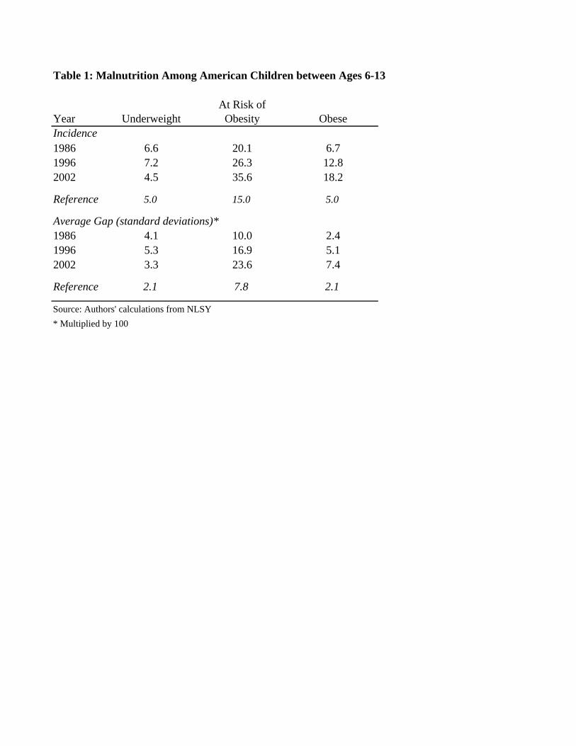
Table 1: Malnutrition Among American Children between Ages 6-13

At Risk ofYear Underweight Obesity ObeseIncidence1986 6.6 20.1 6.71996 7.2 26.3 12.82002 4.5 35.6 18.2

Reference 5.0 15.0 5.0

Average Gap (standard deviations)*1986 4.1 10.0 2.41996 5.3 16.9 5.12002 3.3 23.6 7.4

Reference 2.1 7.8 2.1

Source: Authors' calculations from NLSY* Multiplied by 100

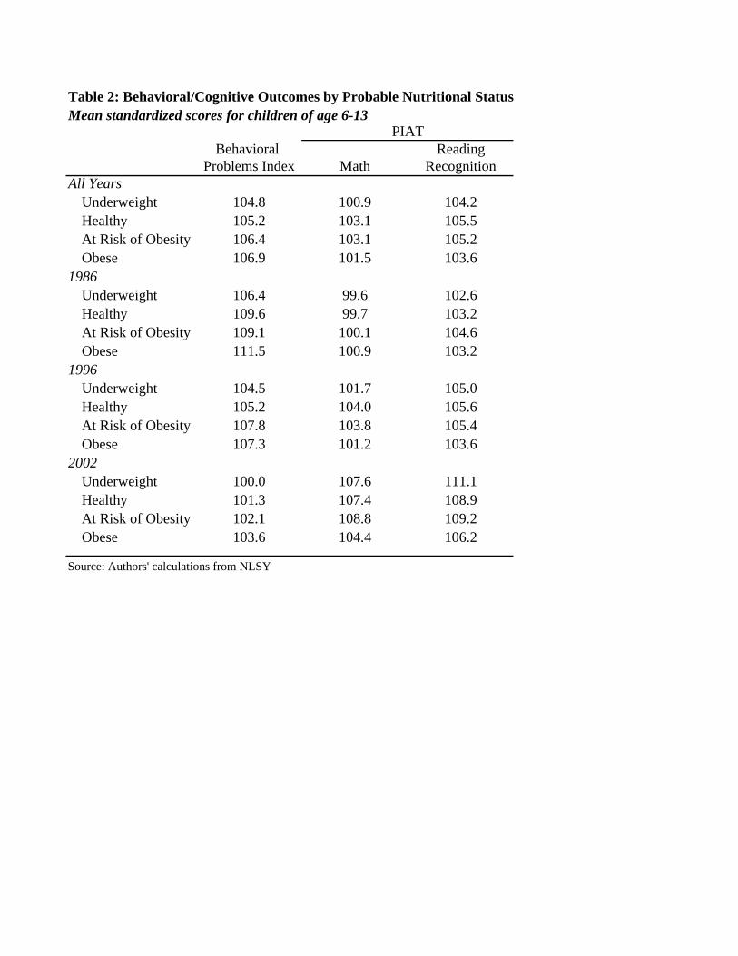
Table 2: Behavioral/Cognitive Outcomes by Probable Nutritional StatusMean standardized scores for children of age 6-13

PIATBehavioral Reading

Problems Index Math RecognitionAll Years

Underweight 104.8 100.9 104.2Healthy 105.2 103.1 105.5At Risk of Obesity 106.4 103.1 105.2Obese 106.9 101.5 103.6

1986Underweight 106.4 99.6 102.6Healthy 109.6 99.7 103.2At Risk of Obesity 109.1 100.1 104.6Obese 111.5 100.9 103.2

1996Underweight 104.5 101.7 105.0Healthy 105.2 104.0 105.6At Risk of Obesity 107.8 103.8 105.4Obese 107.3 101.2 103.6

2002Underweight 100.0 107.6 111.1Healthy 101.3 107.4 108.9At Risk of Obesity 102.1 108.8 109.2Obese 103.6 104.4 106.2

Source: Authors' calculations from NLSY

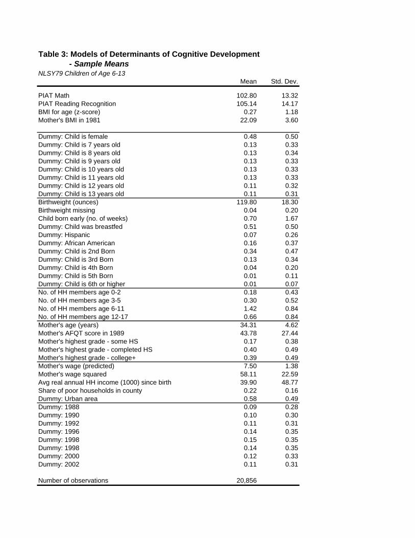
Table 3: Models of Determinants of Cognitive Development - Sample MeansNLSY79 Children of Age 6-13

Mean Std. Dev.

PIAT Math 102.80 13.32PIAT Reading Recognition 105.14 14.17BMI for age (z-score) 0.27 1.18Mother's BMI in 1981 22.09 3.60

Dummy: Child is female 0.48 0.50Dummy: Child is 7 years old 0.13 0.33Dummy: Child is 8 years old 0.13 0.34Dummy: Child is 9 years old 0.13 0.33Dummy: Child is 10 years old 0.13 0.33Dummy: Child is 11 years old 0.13 0.33Dummy: Child is 12 years old 0.11 0.32Dummy: Child is 13 years old 0.11 0.31Birthweight (ounces) 119.80 18.30Birthweight missing 0.04 0.20Child born early (no. of weeks) 0.70 1.67Dummy: Child was breastfed 0.51 0.50Dummy: Hispanic 0.07 0.26Dummy: African American 0.16 0.37Dummy: Child is 2nd Born 0.34 0.47Dummy: Child is 3rd Born 0.13 0.34Dummy: Child is 4th Born 0.04 0.20Dummy: Child is 5th Born 0.01 0.11Dummy: Child is 6th or higher 0.01 0.07No. of HH members age 0-2 0.18 0.43No. of HH members age 3-5 0.30 0.52No. of HH members age 6-11 1.42 0.84No. of HH members age 12-17 0.66 0.84Mother's age (years) 34.31 4.62Mother's AFQT score in 1989 43.78 27.44Mother's highest grade - some HS 0.17 0.38Mother's highest grade - completed HS 0.40 0.49Mother's highest grade - college+ 0.39 0.49Mother's wage (predicted) 7.50 1.38Mother's wage squared 58.11 22.59Avg real annual HH income (1000) since birth 39.90 48.77Share of poor households in county 0.22 0.16Dummy: Urban area 0.58 0.49Dummy: 1988 0.09 0.28Dummy: 1990 0.10 0.30Dummy: 1992 0.11 0.31Dummy: 1996 0.14 0.35Dummy: 1998 0.15 0.35Dummy: 1998 0.14 0.35Dummy: 2000 0.12 0.33Dummy: 2002 0.11 0.31

Number of observations 20,856

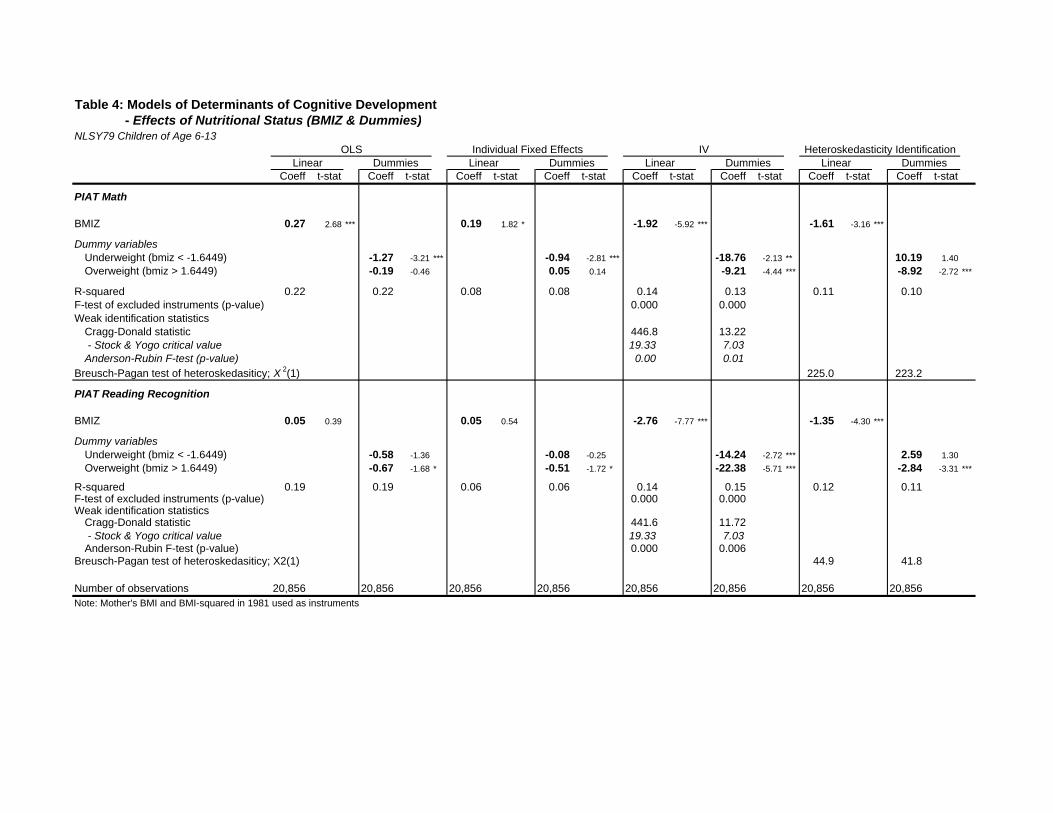
f f f

Table 4: Models of Determinants of Cognitive Development - Effects of Nutritional Status (BMIZ & Dummies)NLSY79 Children of Age 6-13

OLS Individual Fixed Effects IV Heteroskedasticity IdentificationLinear Dummies Linear Dummies Linear Dummies Linear Dummies

Coeff t-stat Coeff t-stat Coeff t-stat Coeff t-stat Coeff t-stat Coef t-stat Coef t-stat Coef t-stat

PIAT Math

BMIZ 0.27 2.68 *** 0.19 1.82 * -1.92 -5.92 *** -1.61 -3.16 ***

Dummy variablesUnderweight (bmiz < -1.6449) -1.27 -3.21 *** -0.94 -2.81 *** -18.76 -2.13 ** 10.19 1.40Overweight (bmiz > 1.6449) -0.19 -0.46 0.05 0.14 -9.21 -4.44 *** -8.92 -2.72 ***

R-squared 0.22 0.22 0.08 0.08 0.14 0.13 0.11 0.10F-test of excluded instruments (p-value) 0.000 0.000Weak identification statistics

Cragg-Donald statistic 446.8 13.22 - Stock & Yogo critical value 19.33 7.03Anderson-Rubin F-test (p-value) 0.00 0.01

Breusch-Pagan test of heteroskedasiticy; X 2(1) 225.0 223.2

PIAT Reading Recognition

BMIZ 0.05 0.39 0.05 0.54 -2.76 -7.77 *** -1.35 -4.30 ***

Dummy variablesUnderweight (bmiz < -1.6449) -0.58 -1.36 -0.08 -0.25 -14.24 -2.72 *** 2.59 1.30Overweight (bmiz > 1.6449) -0.67 -1.68 * -0.51 -1.72 * -22.38 -5.71 *** -2.84 -3.31 ***

R-squared 0.19 0.19 0.06 0.06 0.14 0.15 0.12 0.11F-test of excluded instruments (p-value) 0.000 0.000Weak identification statistics

Cragg-Donald statistic 441.6 11.72 - Stock & Yogo critical value 19.33 7.03Anderson-Rubin F-test (p-value) 0.000 0.006

Breusch-Pagan test of heteroskedasiticy; X2(1) 44.9 41.8

Number of observations 20,856 20,856 20,856 20,856 20,856 20,856 20,856 20,856Note: Mother's BMI and BMI-squared in 1981 used as instruments

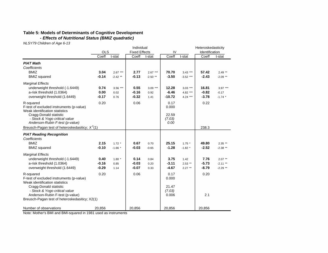
Table 5: Models of Determinants of Cognitive Development - Effects of Nutritional Status (BMIZ quadratic)NLSY79 Children of Age 6-13

Individual HeteroskedasticityOLS Fixed Effects IV Identification

Coeff t-stat Coeff t-stat Coeff t-stat Coeff t-stat

PIAT MathCoefficients

BMIZ 3.04 2.67 *** 2.77 2.67 *** 70.70 3.43 *** 57.42 2.49 **BMIZ squared -0.14 -2.42 ** -0.13 -2.50 ** -3.50 -3.52 *** -2.43 -2.09 **

Marginal Effectsunderweight threshold (-1.6449) 0.74 3.56 *** 0.55 3.09 *** 12.28 3.03 *** 16.81 3.97 ***a-risk threshold (1.0364) 0.00 0.02 -0.16 0.92 -6.46 4.82 *** -0.82 -0.17overweight threshold (1.6449) -0.17 0.76 -0.32 1.41 -10.72 4.24 *** -3.78 -1.74 *

R-squared 0.20 0.06 0.17 0.22F-test of excluded instruments (p-value) 0.000Weak identification statistics

Cragg-Donald statistic 22.59 - Stock & Yogo critical value (7.03)Anderson-Rubin F-test (p-value) 0.00

Breusch-Pagan test of heteroskedasiticy; X 2(1) 238.3

PIAT Reading RecognitionCoefficients

BMIZ 2.15 1.72 * 0.67 0.70 25.15 1.75 * 49.80 2.35 **BMIZ squared -0.10 -1.66 * -0.03 -0.65 -1.28 -1.82 * -2.52 -2.38 **

Marginal Effectsunderweight threshold (-1.6449) 0.40 1.80 * 0.14 0.84 3.75 1.42 7.76 2.07 **a-risk threshold (1.0364) -0.16 0.85 -0.03 0.20 -3.11 2.53 ** -5.73 -2.11 **overweight threshold (1.6449) -0.29 1.14 -0.07 0.33 -4.67 2.27 ** -8.79 -2.29 **

R-squared 0.20 0.06 0.17 0.20F-test of excluded instruments (p-value) 0.000Weak identification statistics

Cragg-Donald statistic 21.47 - Stock & Yogo critical value (7.03)Anderson-Rubin F-test (p-value) 0.006 2.1

Breusch-Pagan test of heteroskedasiticy; X2(1)

Number of observations 20,856 20,856 20,856 20,856Note: Mother's BMI and BMI-squared in 1981 used as instruments

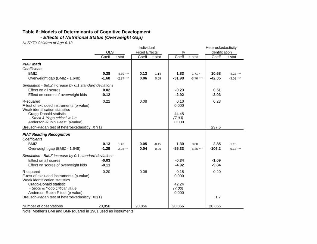
Table 6: Models of Determinants of Cognitive Development - Effects of Nutritional Status (Overweight Gap)NLSY79 Children of Age 6-13

Individual HeteroskedasticityOLS Fixed Effects IV Identification

Coeff t-stat Coeff t-stat Coeff t-stat Coeff t-stat

PIAT MathCoefficients

BMIZ 0.38 4.39 *** 0.13 1.14 1.83 1.71 * 10.68 4.22 ***Overweight gap (BMIZ - 1.648) -1.68 -2.87 *** 0.06 0.09 -31.98 -3.70 *** -42.35 -3.01 ***

Simulation - BMIZ increase by 0.1 standard deviationsEffect on all scores 0.02 -0.23 0.51Effect on scores of overweight kids -0.12 -2.92 -3.03

R-squared 0.22 0.08 0.10 0.23F-test of excluded instruments (p-value) 0.000Weak identification statistics

Cragg-Donald statistic 44.45 - Stock & Yogo critical value (7.03)Anderson-Rubin F-test (p-value) 0.000

Breusch-Pagan test of heteroskedasiticy; X 2(1) 237.5

PIAT Reading RecognitionCoefficients

BMIZ 0.13 1.42 -0.05 -0.45 1.30 0.00 2.85 1.15Overweight gap (BMIZ - 1.648) -1.29 -2.03 ** 0.04 0.06 -55.33 -5.25 *** -106.2 -6.12 ***

Simulation - BMIZ increase by 0.1 standard deviationsEffect on all scores -0.03 -0.34 -1.09Effect on scores of overweight kids -0.11 -4.92 -9.84

R-squared 0.20 0.06 0.15 0.20F-test of excluded instruments (p-value) 0.000Weak identification statistics

Cragg-Donald statistic 42.24 - Stock & Yogo critical value (7.03)Anderson-Rubin F-test (p-value) 0.000

Breusch-Pagan test of heteroskedasiticy; X2(1) 1.7

Number of observations 20,856 20,856 20,856 20,856Note: Mother's BMI and BMI-squared in 1981 used as instruments

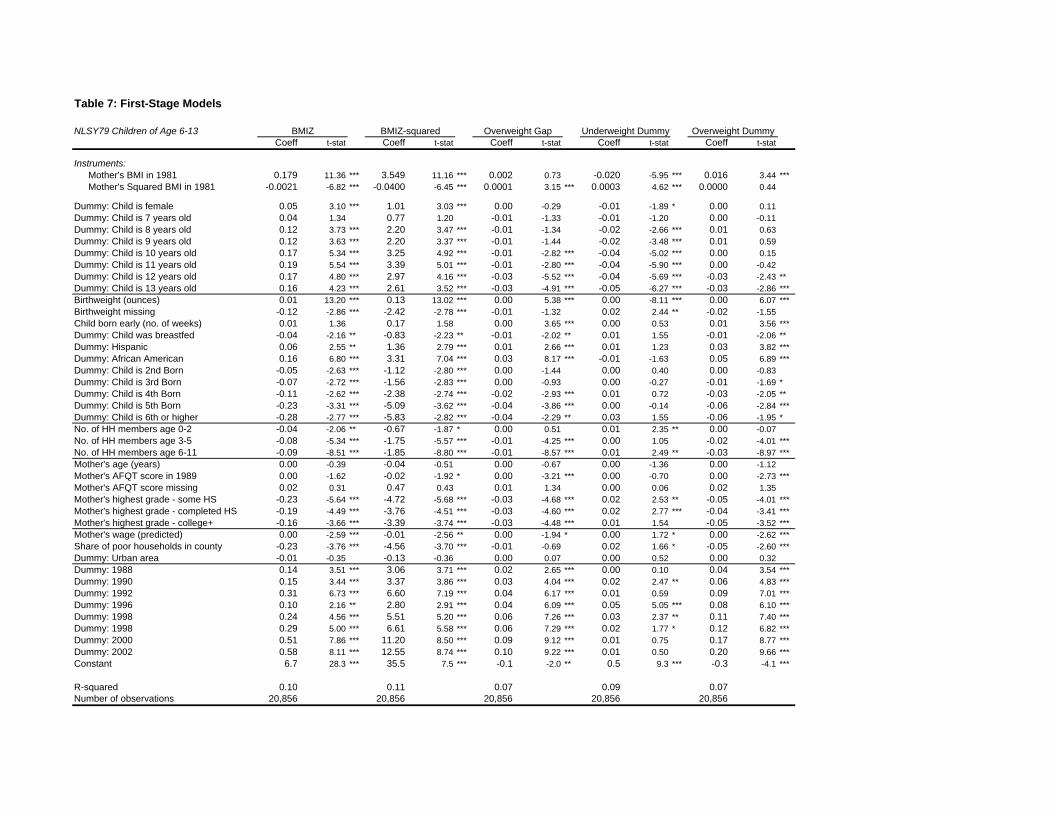
Table 7: First-Stage Models

NLSY79 Children of Age 6-13 BMIZ BMIZ-squared Overweight Gap Underweight Dummy Overweight DummyCoeff t-stat Coeff t-stat Coeff t-stat Coeff t-stat Coeff t-stat

Instruments:Mother's BMI in 1981 0.179 11.36 *** 3.549 11.16 *** 0.002 0.73 -0.020 -5.95 *** 0.016 3.44 ***Mother's Squared BMI in 1981 -0.0021 -6.82 *** -0.0400 -6.45 *** 0.0001 3.15 *** 0.0003 4.62 *** 0.0000 0.44

Dummy: Child is female 0.05 3.10 *** 1.01 3.03 *** 0.00 -0.29 -0.01 -1.89 * 0.00 0.11Dummy: Child is 7 years old 0.04 1.34 0.77 1.20 -0.01 -1.33 -0.01 -1.20 0.00 -0.11Dummy: Child is 8 years old 0.12 3.73 *** 2.20 3.47 *** -0.01 -1.34 -0.02 -2.66 *** 0.01 0.63Dummy: Child is 9 years old 0.12 3.63 *** 2.20 3.37 *** -0.01 -1.44 -0.02 -3.48 *** 0.01 0.59Dummy: Child is 10 years old 0.17 5.34 *** 3.25 4.92 *** -0.01 -2.82 *** -0.04 -5.02 *** 0.00 0.15Dummy: Child is 11 years old 0.19 5.54 *** 3.39 5.01 *** -0.01 -2.80 *** -0.04 -5.90 *** 0.00 -0.42Dummy: Child is 12 years old 0.17 4.80 *** 2.97 4.16 *** -0.03 -5.52 *** -0.04 -5.69 *** -0.03 -2.43 **Dummy: Child is 13 years old 0.16 4.23 *** 2.61 3.52 *** -0.03 -4.91 *** -0.05 -6.27 *** -0.03 -2.86 ***Birthweight (ounces) 0.01 13.20 *** 0.13 13.02 *** 0.00 5.38 *** 0.00 -8.11 *** 0.00 6.07 ***Birthweight missing -0.12 -2.86 *** -2.42 -2.78 *** -0.01 -1.32 0.02 2.44 ** -0.02 -1.55Child born early (no. of weeks) 0.01 1.36 0.17 1.58 0.00 3.65 *** 0.00 0.53 0.01 3.56 ***Dummy: Child was breastfed -0.04 -2.16 ** -0.83 -2.23 ** -0.01 -2.02 ** 0.01 1.55 -0.01 -2.06 **Dummy: Hispanic 0.06 2.55 ** 1.36 2.79 *** 0.01 2.66 *** 0.01 1.23 0.03 3.82 ***Dummy: African American 0.16 6.80 *** 3.31 7.04 *** 0.03 8.17 *** -0.01 -1.63 0.05 6.89 ***Dummy: Child is 2nd Born -0.05 -2.63 *** -1.12 -2.80 *** 0.00 -1.44 0.00 0.40 0.00 -0.83Dummy: Child is 3rd Born -0.07 -2.72 *** -1.56 -2.83 *** 0.00 -0.93 0.00 -0.27 -0.01 -1.69 *Dummy: Child is 4th Born -0.11 -2.62 *** -2.38 -2.74 *** -0.02 -2.93 *** 0.01 0.72 -0.03 -2.05 **Dummy: Child is 5th Born -0.23 -3.31 *** -5.09 -3.62 *** -0.04 -3.86 *** 0.00 -0.14 -0.06 -2.84 ***Dummy: Child is 6th or higher -0.28 -2.77 *** -5.83 -2.82 *** -0.04 -2.29 ** 0.03 1.55 -0.06 -1.95 *No. of HH members age 0-2 -0.04 -2.06 ** -0.67 -1.87 * 0.00 0.51 0.01 2.35 ** 0.00 -0.07No. of HH members age 3-5 -0.08 -5.34 *** -1.75 -5.57 *** -0.01 -4.25 *** 0.00 1.05 -0.02 -4.01 ***No. of HH members age 6-11 -0.09 -8.51 *** -1.85 -8.80 *** -0.01 -8.57 *** 0.01 2.49 ** -0.03 -8.97 ***Mother's age (years) 0.00 -0.39 -0.04 -0.51 0.00 -0.67 0.00 -1.36 0.00 -1.12Mother's AFQT score in 1989 0.00 -1.62 -0.02 -1.92 * 0.00 -3.21 *** 0.00 -0.70 0.00 -2.73 ***Mother's AFQT score missing 0.02 0.31 0.47 0.43 0.01 1.34 0.00 0.06 0.02 1.35Mother's highest grade - some HS -0.23 -5.64 *** -4.72 -5.68 *** -0.03 -4.68 *** 0.02 2.53 ** -0.05 -4.01 ***Mother's highest grade - completed HS -0.19 -4.49 *** -3.76 -4.51 *** -0.03 -4.60 *** 0.02 2.77 *** -0.04 -3.41 ***Mother's highest grade - college+ -0.16 -3.66 *** -3.39 -3.74 *** -0.03 -4.48 *** 0.01 1.54 -0.05 -3.52 ***Mother's wage (predicted) 0.00 -2.59 *** -0.01 -2.56 ** 0.00 -1.94 * 0.00 1.72 * 0.00 -2.62 ***Share of poor households in county -0.23 -3.76 *** -4.56 -3.70 *** -0.01 -0.69 0.02 1.66 * -0.05 -2.60 ***Dummy: Urban area -0.01 -0.35 -0.13 -0.36 0.00 0.07 0.00 0.52 0.00 0.32Dummy: 1988 0.14 3.51 *** 3.06 3.71 *** 0.02 2.65 *** 0.00 0.10 0.04 3.54 ***Dummy: 1990 0.15 3.44 *** 3.37 3.86 *** 0.03 4.04 *** 0.02 2.47 ** 0.06 4.83 ***Dummy: 1992 0.31 6.73 *** 6.60 7.19 *** 0.04 6.17 *** 0.01 0.59 0.09 7.01 ***Dummy: 1996 0.10 2.16 ** 2.80 2.91 *** 0.04 6.09 *** 0.05 5.05 *** 0.08 6.10 ***Dummy: 1998 0.24 4.56 *** 5.51 5.20 *** 0.06 7.26 *** 0.03 2.37 ** 0.11 7.40 ***Dummy: 1998 0.29 5.00 *** 6.61 5.58 *** 0.06 7.29 *** 0.02 1.77 * 0.12 6.82 ***Dummy: 2000 0.51 7.86 *** 11.20 8.50 *** 0.09 9.12 *** 0.01 0.75 0.17 8.77 ***Dummy: 2002 0.58 8.11 *** 12.55 8.74 *** 0.10 9.22 *** 0.01 0.50 0.20 9.66 ***Constant 6.7 28.3 *** 35.5 7.5 *** -0.1 -2.0 ** 0.5 9.3 *** -0.3 -4.1 ***

R-squared 0.10 0.11 0.07 0.09 0.07Number of observations 20,856 20,856 20,856 20,856 20,856

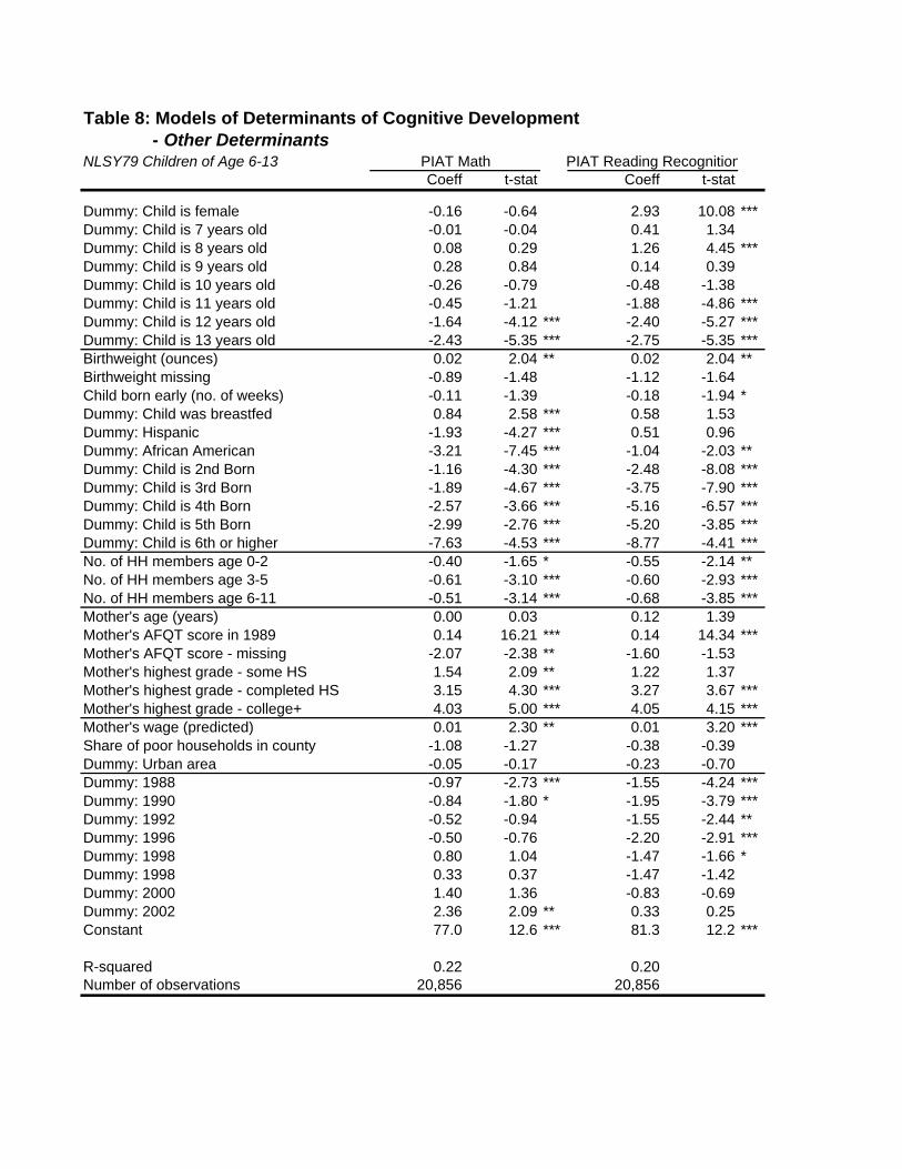
n

Table 8: Models of Determinants of Cognitive Development - Other DeterminantsNLSY79 Children of Age 6-13 PIAT Math PIAT Reading Recognitio

Coeff t-stat Coeff t-stat

Dummy: Child is female -0.16 -0.64 2.93 10.08 ***Dummy: Child is 7 years old -0.01 -0.04 0.41 1.34Dummy: Child is 8 years old 0.08 0.29 1.26 4.45 ***Dummy: Child is 9 years old 0.28 0.84 0.14 0.39Dummy: Child is 10 years old -0.26 -0.79 -0.48 -1.38Dummy: Child is 11 years old -0.45 -1.21 -1.88 -4.86 ***Dummy: Child is 12 years old -1.64 -4.12 *** -2.40 -5.27 ***Dummy: Child is 13 years old -2.43 -5.35 *** -2.75 -5.35 ***Birthweight (ounces) 0.02 2.04 ** 0.02 2.04 **Birthweight missing -0.89 -1.48 -1.12 -1.64Child born early (no. of weeks) -0.11 -1.39 -0.18 -1.94 *Dummy: Child was breastfed 0.84 2.58 *** 0.58 1.53Dummy: Hispanic -1.93 -4.27 *** 0.51 0.96Dummy: African American -3.21 -7.45 *** -1.04 -2.03 **Dummy: Child is 2nd Born -1.16 -4.30 *** -2.48 -8.08 ***Dummy: Child is 3rd Born -1.89 -4.67 *** -3.75 -7.90 ***Dummy: Child is 4th Born -2.57 -3.66 *** -5.16 -6.57 ***Dummy: Child is 5th Born -2.99 -2.76 *** -5.20 -3.85 ***Dummy: Child is 6th or higher -7.63 -4.53 *** -8.77 -4.41 ***No. of HH members age 0-2 -0.40 -1.65 * -0.55 -2.14 **No. of HH members age 3-5 -0.61 -3.10 *** -0.60 -2.93 ***No. of HH members age 6-11 -0.51 -3.14 *** -0.68 -3.85 ***Mother's age (years) 0.00 0.03 0.12 1.39Mother's AFQT score in 1989 0.14 16.21 *** 0.14 14.34 ***Mother's AFQT score - missing -2.07 -2.38 ** -1.60 -1.53Mother's highest grade - some HS 1.54 2.09 ** 1.22 1.37Mother's highest grade - completed HS 3.15 4.30 *** 3.27 3.67 ***Mother's highest grade - college+ 4.03 5.00 *** 4.05 4.15 ***Mother's wage (predicted) 0.01 2.30 ** 0.01 3.20 ***Share of poor households in county -1.08 -1.27 -0.38 -0.39Dummy: Urban area -0.05 -0.17 -0.23 -0.70Dummy: 1988 -0.97 -2.73 *** -1.55 -4.24 ***Dummy: 1990 -0.84 -1.80 * -1.95 -3.79 ***Dummy: 1992 -0.52 -0.94 -1.55 -2.44 **Dummy: 1996 -0.50 -0.76 -2.20 -2.91 ***Dummy: 1998 0.80 1.04 -1.47 -1.66 *Dummy: 1998 0.33 0.37 -1.47 -1.42Dummy: 2000 1.40 1.36 -0.83 -0.69Dummy: 2002 2.36 2.09 ** 0.33 0.25Constant 77.0 12.6 *** 81.3 12.2 ***

R-squared 0.22 0.20Number of observations 20,856 20,856

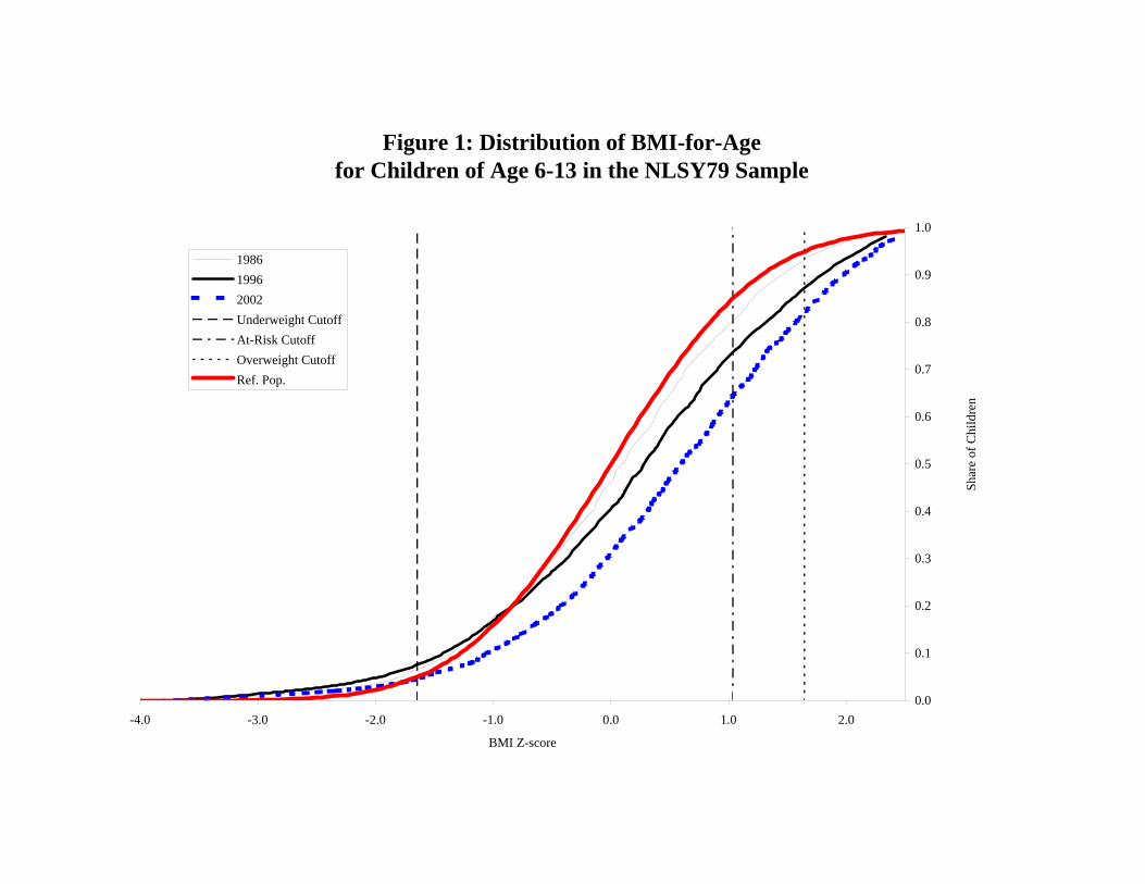
Figure 1: Distribution of BMI-for-Age for Children of Age 6-13 in the NLSY79 Sample

0.0

0.1

0.2

0.3

0.4

0.5

0.6

0.7

0.8

0.9

1.0

-4.0 -3.0 -2.0 -1.0 0.0 1.0 2.0

BMI Z-score

Shar

e of

Chi

ldre

n

198619962002Underweight CutoffAt-Risk CutoffOverweight CutoffRef. Pop.

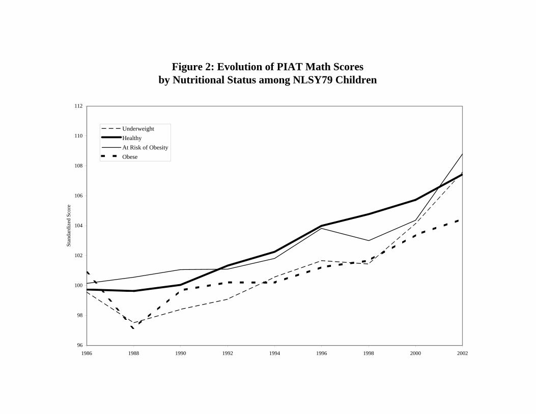
Figure 2: Evolution of PIAT Math Scoresby Nutritional Status among NLSY79 Children

96

98

100

102

104

106

108

110

112

1986 1988 1990 1992 1994 1996 1998 2000 2002

Stan

dard

ized

Sco

re

UnderweightHealthyAt Risk of ObesityObese

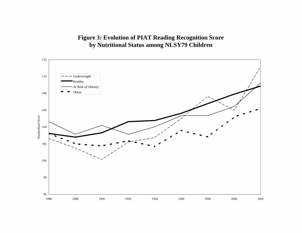
Figure 3: Evolution of PIAT Reading Recognition Scoreby Nutritional Status among NLSY79 Children

96

98

100

102

104

106

108

110

112

1986 1988 1990 1992 1994 1996 1998 2000 2002

Stan

dard

ized

Sco

re

UnderweightHealthyAt Risk of ObesityObese