Institute for Research on Poverty Discussion Paper no. 1321-07

Food Stamps and Food Insecurity: What Can Be Learned in the Presence of Nonclassical Measurement Error?

Craig Gundersen Iowa State University

E-mail: cggunder@iastate.edu

Brent Kreider Iowa State University

E-mail: bkreider@iastate.edu

February 2007 This research is funded through a Research Innovation and Development Grant in Economics (RIDGE) from the U.S. Department of Agriculture’s (USDA) Economic Research Service administered through the Institute for Research on Poverty (IRP) at the University of Wisconsin–Madison. The views expressed in this article are solely those of the authors. Previous versions of this paper were presented at the Annual Meetings of the Association for Public Policy Analysis and Management, the IRP-USDA Small Grants Research Workshop, the Annual Meetings of the Population Association of America, the Annual Meetings of the American Council on Consumer Interests, and the RIDGE Conference. The authors wish to thank participants at the above venues and, in particular, Karl Scholz, Mark Nord, Hugette Sun, and Sandi Hoffereth. IRP Publications (discussion papers, special reports, and the newsletter Focus) are available on the Internet. The IRP Web site can be accessed at the following address: http://www.irp.wisc.edu

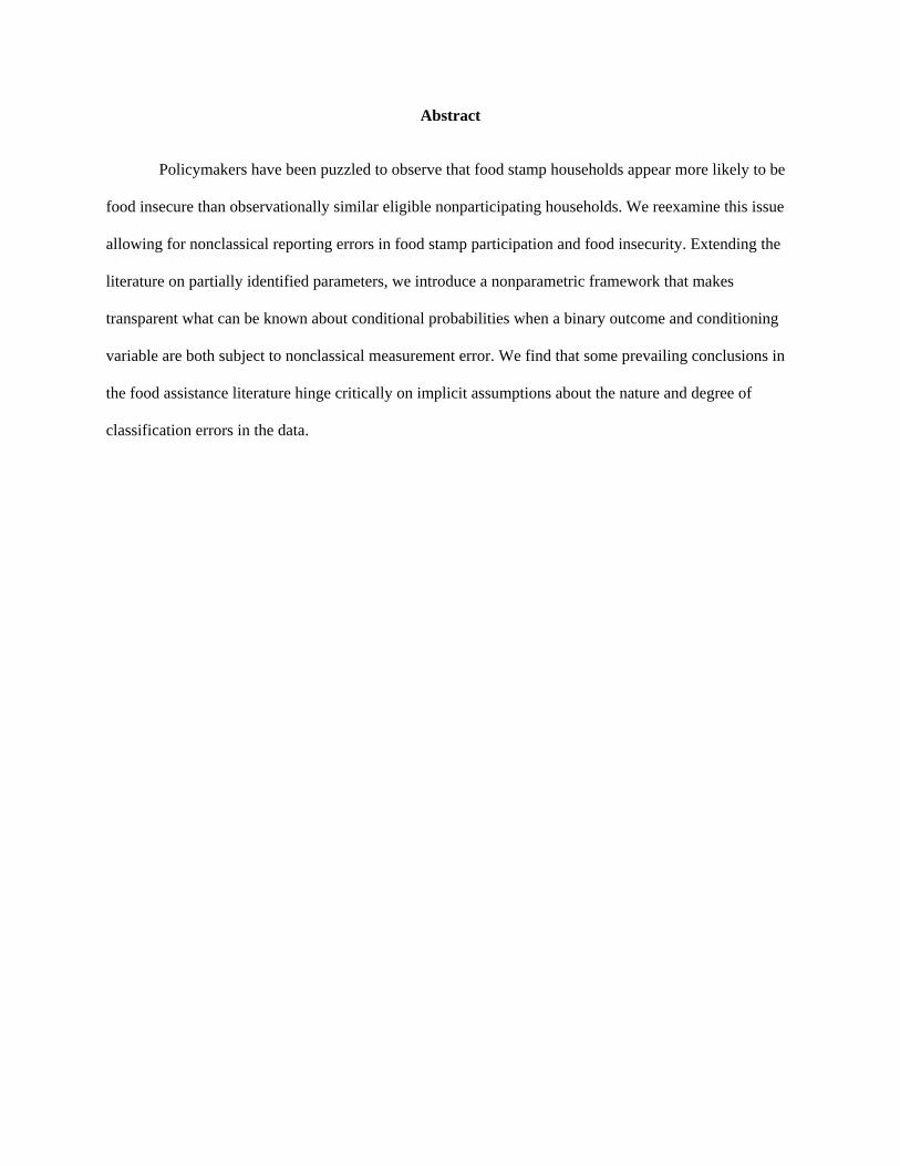
Abstract

Policymakers have been puzzled to observe that food stamp households appear more likely to be

food insecure than observationally similar eligible nonparticipating households. We reexamine this issue

allowing for nonclassical reporting errors in food stamp participation and food insecurity. Extending the

literature on partially identified parameters, we introduce a nonparametric framework that makes

transparent what can be known about conditional probabilities when a binary outcome and conditioning

variable are both subject to nonclassical measurement error. We find that some prevailing conclusions in

the food assistance literature hinge critically on implicit assumptions about the nature and degree of

classification errors in the data.

1 Introduction

The largest food assistance program in the United States, the Food Stamp Program is �. . . the most critical

component of the safety net against hunger (U.S. Department of Agriculture, 1999, p.7).�While this program

provides basic protection for citizens of all ages and household status, the safety net is especially important

for children who comprise over half of all recipients (Cunnyngham and Brown, 2004). Given the cornerstone

role of food stamps in ensuring food security, policymakers have been puzzled to observe that food stamp

households with children are more likely to be food insecure than observationally similar nonparticipating

eligible households. In response to a burgeoning interest in food insecurity, an extensive literature has

developed in the last decade on the determinants and consequences of food insecurity in the United States

(for recent work see, e.g., Bhattacharya et al., 2004; Bitler et al., 2005; Borjas, 2004; Dunifon and Kowaleski-

Jones, 2003; Furness et al., 2004; Gundersen et al., 2003; Laraia et al., 2006; Ribar and Hamrick, 2003; Van

Hook and Balistreri, 2006).

The negative association between food security and food stamp participation has been ascribed to several

factors including self-selection (those most at risk of food insecurity are more likely to receive food stamps),

the timing of food insecurity versus food stamp receipt (someone might have been food insecure and then

entered the Food Stamp Program), misreporting of food insecurity status, and misreporting of food stamp

receipt. Previous work has studied these �rst two issues (e.g., Gundersen and Oliveira, 2001; Nord et al.,

2004). The literature has not assessed the consequences of measurement error.

We focus on measurement error issues using data from the Core Food Security Module (CFSM), a

component of the Current Population Survey (CPS). Speci�cally, we investigate what can be inferred when

food stamp participation and food insecurity status may be misreported. As elaborated below, we extend the

econometric literature on misclassi�ed binary variables by studying identi�cation when an outcome (in our

case food insecurity) and a conditioning variable (food stamp participation) are both subject to arbitrary

endogenous classi�cation error. We also consider the identifying power of assumptions that restrict the

patterns of classi�cation errors. For example, misreported food insecurity status might arise independently

of true food stamp participation status.

A number of studies have documented the presence of substantial reporting error in households�receipt of

food stamp bene�ts. For example, using administrative data matched with data from the Survey of Income

1

and Program Participation (SIPP), Marquis and Moore (1990) found that about 19 percent of actual food

stamp recipient households reported that they were not recipients. Underreporting of up to 25 percent has

also been documented in comparisons between responses in surveys, such as the CPS, and administrative

data (Cunnyngham, 2005). Bollinger and David (1997, 2001, 2005) estimate econometric models of food

stamp response errors and study the consequences of misreporting for inference on take-up rates.

The assumption of fully accurate reporting of food insecurity status can also be questioned. For example,

some food stamp recipients might misreport being food insecure if they believe that to report otherwise could

jeopardize their eligibility.1 Alternatively, some parents may misreport being food secure if they feel ashamed

about heading a household in which their children are not getting enough food to eat (Hamelin et al., 2002).

More generally, some of the survey questions used to calculate o¢ cial food insecurity status (see Section 2)

require the respondent to make a subjective judgment. Validation studies consistently reveal large degrees

of response error in survey data for a wide range of self-reports, even for relatively objective variables.2 As

is well understood in the econometrics literature, even random errors can lead to seriously biased parameter

estimates.

In this paper, we study inferences in an environment that allows for the possibility of misclassi�ed food

stamp participation and food insecurity status. Extending the literature on misclassi�ed binary variables

(e.g., Aigner, 1973; Bollinger, 1996; Bollinger and David, 1997, 2001; Frazis and Loewenstein, 2003; Kreider

and Pepper, forthcoming), we introduce a nonparametric approach for assessing what can be inferred when

binary outcomes may be misclassi�ed. In this environment, we allow for the possibility that food stamp

participation errors are endogenously related to the food insecurity outcome. Our framework follows the

spirit of Horowitz and Manski (1995) who study partial identi�cation under corrupt samples given minimal

assumptions on the error generating process.3

Within this environment, we derive sharp worst-case bounds that exploit all available information under

1Other literatures contain lively debates about the extent to which self-reported disability might be in�uenced bya respondent�s desire to rationalize labor force withdrawal or the receipt of disability bene�ts (see, e.g., Bound andBurkhauser, 1999).

2Black et al. (2003), for example, �nd that more than a third of respondents to the U.S. Census claiming to holda professional degree have no such degree, with widely varying patterns of false positives and false negatives acrossdemographic groups. In matched data, Barron et al. (1997) �nd that the correlation between worker-reported trainingand employer-reporting training is less than 0:4 and Berger et al. (1998) report that more than a �fth of workers andtheir employers disagree about whether the worker was eligible for health insurance through the employer; see alsoBerger et al. (2000).

3For extensions of their nonparametric approach, see, for example, Ginther (2000), Pepper (2000), Dominitz andSherman (2004), Molinari (2005), and Kreider and Pepper (forthcoming).

2

the maintained assumptions. To �rst isolate the identi�cation problem associated with potentially misre-

ported food stamp participation, we begin our analysis by assuming that the food insecurity outcome is

reported without error. As a reference case, we derive easy-to-compute sharp bounds on conditional food

insecurity prevalence rates when food stamp misreporting arises independently of true participation status.

We show how to transform a computationally expensive multidimensional search problem into a series of

single-dimension search problems that requires little programming e¤ort or computational time. We compare

these bounds to those obtained under alternative assumptions on the nature of reporting error. For exam-

ple, we can consider the possibility that respondents are prone to underreport but not overreport program

participation. In the most general case, we make no assumptions about the patterns of classi�cation errors.

After studying the identi�cation problem for the case of fully accurate food insecurity responses, we consider

the case that food insecurity as well as food stamp participation may be reported with error.

In the next section, we describe the central variables of interest in this paper �food insecurity and food

stamps �followed by a description of the CFSM data. In Section 3, we highlight the statistical identi�cation

problem created by the potential unreliability of the self-reported data. Applying and extending methods

from a rapidly emerging literature on partially identi�ed probability distributions (see Manski, 2003 for

a unifying discussion), Section 4 shows how conditional food insecurity prevalence rates can be partially

identi�ed under various restrictions on the nature and degree of classi�cation errors. Section 5 presents our

empirical results and Section 6 concludes.

2 Concepts and Data

2.1 Food Insecurity

The extent of food insecurity in the United States has become a well-publicized issue of concern to policy-

makers and program administrators. In 2003, 11:2% of the U.S. population reported that they su¤ered from

food insecurity. As described below, these households were uncertain of having, or unable to acquire, enough

food for all their members because they had insu¢ cient money or other resources. About 3:5% su¤ered from

self-reported food insecurity with hunger. These households reported hunger at some time during the year

because they could not a¤ord enough food. For households with children, the reported levels are higher �

16:7% and 3:8% respectively.

3

To calculate the o¢ cial food insecurity rates in the U.S., a series of 18 questions are posed in the CSFM

for families with children. (For families without children and for households with one individual, a subset

of 10 of these questions are posed.) Each question is designed to capture some aspect of food insecurity

and, for some questions, the frequency with which it manifests itself. Examples include �I worried whether

our food would run out before we got money to buy more� (the least severe outcome); �Did you or the

other adults in your household ever cut the size of your meals or skip meals because there wasn�t enough

money for food;� �Were you ever hungry but did not eat because you couldn�t a¤ord enough food;� and

�Did a child in the household ever not eat for a full day because you couldn�t a¤ord enough food�(the most

severe outcome). A household with children is categorized as (a) food secure if the respondent responds

a¢ rmatively to two or fewer of these questions; (b) food insecure if the respondent responds a¢ rmatively to

three or more questions; and (c) food insecure with hunger if the respondent responds a¢ rmatively to eight

or more questions.4 A complete listing of the food insecurity questions can be found in Nord et al. (2005).

The CFSM questions are designed to portray food insecurity in the United States in a manner consistent

with how experts perceive the presence of food insecurity. Given conceptual di¢ culties in quantifying food

insecurity status, its measurement contains both objective and subjective components.5 Such classi�cations

are thus akin to classi�cations of work disability insofar as work capacity involves both objective factors (e.g.,

the presence of a medical condition) and subjective factors (e.g., the ability to function e¤ectively despite

the presence of the condition).6 For reasons described above, a household�s food insecurity status might be

misclassi�ed relative to the profession�s intended threshold for true food insecurity.

2.2 The Food Stamp Program

The Food Stamp Program, with a few exceptions, is available to all families with children who meet income

and asset tests. To receive food stamps, households must meet three �nancial criteria: a gross-income test,

4The label �food insecurity with hunger�has been criticized by some for its measure of well-being at the householdlevel rather than at the individual level (National Research Council, 2006). We nevertheless focus on this measurebecause it continues to be utilized as a descriptor in the o¢ cial statistics of food insecurity in the United States (e.g.,Nord et al., 2005). We treat food insecurity as a binary indicator in this paper consistent with how it is generallyde�ned by researchers and policymakers. We do not attempt to address conceptual issues about how food insecurityshould be ideally quanti�ed.

5Consistent with the subjective nature of the questions in the CFSM, Gundersen and Ribar (2005) �nd that self-reported food insecurity has a substantially higher correlation with a subjective measure of food expenditure needsthan with an objective measure of such needs.

6See, for example, Bound (1991).

4

a net-income test, and an asset test. A household�s gross income before taxes in the previous month cannot

exceed 130 percent of the poverty line, and net monthly income cannot exceed the poverty line.7 Finally,

income-eligible households with assets less than $2,000 qualify for the program. The value of a vehicle

above $4,650 is considered an asset unless it is used for work or for the transportation of disabled persons.

Households receiving Temporary Assistance for Needy Families (TANF) and households where all members

receive Supplemental Security Income (SSI) are categorically eligible for food stamps and do not have to

meet these three tests.

A large fraction of households eligible for food stamps do not participate. This outcome is often ascribed

to three main factors. First, there may be stigma associated with receiving food stamps. Stigma encompasses

a wide variety of sources, from a person�s own distaste for receiving food stamps to the fear of disapproval

from others when redeeming food stamps to the possible negative reaction of caseworkers (Ranney and

Kushman, 1987; Mo¢ tt, 1983). Second, transaction costs can diminish the attractiveness of participation.8

A household faces these costs on a repeated basis when it must recertify its eligibility. Third, against these

costs, the bene�t level may be too small to induce participation; food stamp bene�ts can be as low as $10 a

month for a family.

Reported food stamp participation in survey data may deviate from actual participation. Evidence of this

underreporting has surfaced in two types of studies, both of which compare self-reported information with

o¢ cial records. The �rst type has compared aggregate statistics obtained from self-reported survey data with

those obtained from administrative data. These studies suggest the presence of substantial underreporting

of food stamp recipiency. In the CFSM data used in our analysis, Bitler et al. (2003, Table 3) �nd that

the number of food stamp recipients in the 1999 CFSM re�ected only about 85 percent of the true number

according to administrative data. Similar undercounts have been observed in the March Supplement of the

CPS, the Survey of Income and Program Participation (SIPP), the Panel Study of Income Dynamics (PSID),

and the Consumer Expenditure Survey (Trippe et al., 1992). Other studies have compared individual reports

of food stamp participation status in surveys with matched reports from administrative data. Using this

7Net income is calculated by subtracting a standard deduction from a household�s gross income. In addition tothis standard deduction, households with labor earnings deduct 20 percent of those earnings from their gross income.Deductions are also taken for child care and/or care for disabled dependents, medical expenses, and excessive shelterexpenses.

8Examples of such costs include travel time to a food stamp o¢ ce and time spent in the o¢ ce, the burden oftransporting children to the o¢ ce or paying for child care services, and the direct costs of paying for transportation.

5

method, researchers can identify both false positive errors of commission (i.e., reporting bene�ts not actually

received) and false negative errors of omission (i.e., not reporting bene�ts actually received). Using data

from the SIPP, Bollinger and David (1997, Table 2) �nd, consistent with aggregate reports, that 0:3 percent

of households have errors of commission while 12:0 percent have errors of omission.

2.3 Data

Our analysis uses data from the December Supplement of the 2003 CPS. The CPS is the o¢ cial data source

for poverty and unemployment rates in the U.S. and has included the CFSM component at least one month

in every year since 1995. In 2003, this component was included in the December Supplement. The December

CPS also contains information on food stamp participation status. We limit our sample to households will

children eligible for the Food Stamp Program based on the gross income criterion. Our sample of 2707

observations consists of all households with children reporting incomes less than 130 percent of the poverty

line.9

Table 1 displays joint frequency distributions of reported food insecurity status and food stamp participa-

tion among eligible households. Panel A shows that 52:3% of eligible households with children who reported

the receipt of food stamps also reported being food insecure. Among eligible households who did not report

the receipt of food stamps, 34:4% reported being food insecure. Based on these responses, the prevalence

of food insecurity is 17:9 percentage points higher among food stamp recipients than among nonrecipients.

Based on analogous information in Panel B, the prevalence of food insecurity with hunger is 6:5 percentage

points higher among food stamp recipients (15:9%) than among nonrecipients (9:4%). In what follows, we

assess what can be inferred about these conditional prevalence rates when food stamp participation and food

insecurity status are subject to classi�cation errors.

9Our data do not contain su¢ cient information for us to apply the net income test or asset test. However,virtually all families meeting the gross income test also meet the net income test. The asset test could be importantfor a sample that includes a high proportion of households headed by an elderly person (Haider et al., 2003). Forhouseholds with children, however, the fraction asset ineligible but gross income eligible is small. Using combineddata from 1989 to 2004 in the March CPS (which does have information on the returns to assets), Gundersen andO¤utt (2005) �nd that only 7:1% of households are asset ineligible but gross income eligible.

6

3 Identi�cation

To assess the impact of classi�cation error on inferences, we introduce notation that distinguishes between

reported food stamp participation status and true participation status. Let X� = 1 indicate that a household

truly receives food stamps, with X� = 0 otherwise. Instead of observing X�, we observe a self-reported

counterpart X. A latent variable Z� indicates whether a report is accurate: Z� = 1 if X� = X, with

Z� = 0 otherwise. Finally, let Y = 1 denote that a household reports being food insecure, with Y = 0

otherwise. Initially, we focus exclusively on food stamp misclassi�cations and assume that food insecurity

status is measured without error. We later allow for the possibility of misclassi�cations in both food stamp

participation and food insecurity status.

Taking self-reports at face value, we can point-identify the food insecurity prevalence rates among food

stamp recipients and nonrecipients as 0:523 and 0:344, respectively (Table 1A) �a di¤erence that is statisti-

cally signi�cant at better than the 1% level. Allowing for the possibility of classi�cation errors, however, we

cannot identify P (Y = 1jX�) even if reporting errors are thought to occur randomly. To formalize the iden-

ti�cation problem, consider the rate of food insecurity among the true population of food stamp recipients.

This conditional probability is given by

P (Y = 1jX� = 1) =P (Y = 1; X� = 1)

P (X� = 1). (1)

Since one does not observe X�, neither the numerator nor the denominator is identi�ed.10 However,

assumptions on the pattern of reporting errors can place restrictions on relationships between the unobserved

quantities. Let �+1 � P (Y = 1; X = 1; Z� = 0) and ��1 � P (Y = 1; X = 0; Z� = 0) denote the fraction of

false positive and false negative food stamp participation classi�cations, respectively, within the population of

food-insecure households. Similarly, let �+0 � P (Y = 0; X = 1; Z� = 0) and ��0 � P (Y = 0; X = 0; Z� = 0)

denote the fraction of false positive and false negative food stamp participation classi�cations, respectively,

within the population of food-secure households. Then we can decompose the numerator and denominator

10For ease of exposition, our notation leaves implicit any other conditioning variables.

7

in (1) into identi�ed and unidenti�ed quantities:

P (Y = 1jX� = 1) =p11 + �

�1 � �+1

p+���1 + �

�0

����+1 + �

+0

� (2)

where p11 � P (Y = 1; X = 1) and p � P (X = 1) are identi�ed by the data and the remaining quantities are

not identi�ed. In the numerator, ��1 � �+1 re�ects the unobserved excess of false negative vs. false positive

food stamp participation reports within the population of food-insecure households. In the denominator,���1 + �

�0

����+1 + �

+0

�re�ects the unobserved excess of false positive vs. false negative classi�cations within

the entire population of interest. The food insecurity prevalence rate among nonrecipients can be written

analogously as

P (Y = 1jX� = 0) =p10 + �

+1 � ��1

1� p+��+1 + �

+0

�����1 + �

�0

� (3)

where p10 � P (Y = 1; X = 0).

Worst-case bounds on P (Y = 1jX�) are obtained by �nding the extrema of equations (2) and (3) subject

to restrictions on the false positives and false negatives �+1 , �+0 , �

�1 , and �

�0 . Without assumptions on the

nature of reporting errors, the following constraints hold:

(i) 0 � �+1 � P (Y = 1; X = 1) � p11

(ii) 0 � �+0 � P (Y = 0; X = 1) � p01

(iii) 0 � ��1 � P (Y = 1; X = 0) � p10

(iv) 0 � ��0 � P (Y = 0; X = 0) � p00.

For example, the fraction of food insecure households that falsely reports receiving food stamps obviously

cannot exceed the fraction of food insecure households that reports receiving food stamps.

Before considering any structure on the pattern of false positives and false negatives, we begin by assessing

identi�cation given a limit on the potential degree of misclassi�cation. Following Horowitz and Manski (1995)

and the literature on robust statistics (e.g., Huber 1981), we can study how identi�cation of an unknown

parameter varies with the con�dence in the data. Consider an upper bound, q, on the fraction of inaccurate

8

food stamp participation classi�cations: P (Z� = 0) � q which implies

(v) �+1 + �+0 + �

�1 + �

�0 � q.

This assumption incorporates a researcher�s beliefs about the potential degree of data corruption. If

q equals 0 (as is implicitly assumed in all previous work on food insecurity), then P (Y = 1jX�) is point-

identi�ed because all food stamp participation reports are assumed to be accurate. At the opposite extreme,

a researcher unwilling to place any limit on the potential degree of reporting error can set q equal to 1. In

that case, there is no hope of learning anything about P (Y = 1jX�) without constraining the pattern of

reporting errors. In any event, the sensitivity of inferences on P (Y = 1jX�) can be examined by varying the

value of q between 0 and 1.

In the �corrupt sampling� case in which nothing is known about the pattern of reporting errors, we

compute sharp bounds on P (Y = 1jX�) using a result from Kreider and Pepper (forthcoming). After brie�y

presenting these bounds, we derive a narrower set of bounds obtained under the assumption that classi�cation

errors arise independently of true participation status. We also consider the identifying power of other

assumptions. For example, we assess what can be known about these parameters under an asymmetric errors

assumption that households may underreport food stamp participation but do not falsely report receiving

bene�ts. This assumption is consistent with the evidence discussed above regarding errors of omission and

errors of commission (Bollinger and David, 2001). After establishing sets of bounds on P (Y = 1jX�) for

the case that food insecurity is accurately reported, we allow for the possibility that food insecurity status

may also be misreported. Throughout this analysis, we do not impose the nondi¤erential errors assumption

embedded in the classical errors-in-variables framework.11

11 In our context, this assumption would require that, conditional on true participation status, participation classi�-cation errors arise independently of food insecurity status. Bollinger (1996) studies identi�cation of a mean regressionwhen a potentially mismeasured binary conditioning variable satis�es the nondi¤erential errors assumption. In con-trast to our nonparametric approach, Hausman et al. (1998) propose parametric and semiparametric estimators in adiscrete-response regression setting that account for misclassi�cation in a dependent variable.

9

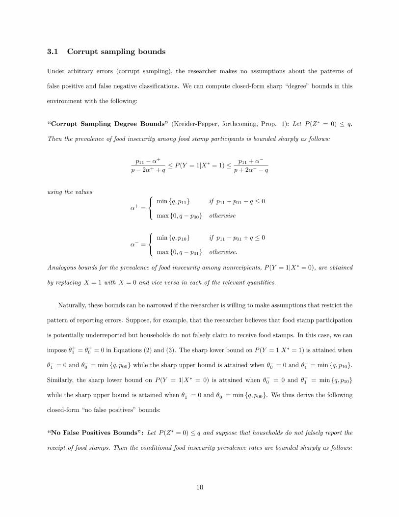
3.1 Corrupt sampling bounds

Under arbitrary errors (corrupt sampling), the researcher makes no assumptions about the patterns of

false positive and false negative classi�cations. We can compute closed-form sharp �degree�bounds in this

environment with the following:

�Corrupt Sampling Degree Bounds� (Kreider-Pepper, forthcoming, Prop. 1): Let P (Z� = 0) � q.

Then the prevalence of food insecurity among food stamp participants is bounded sharply as follows:

p11 � �+p� 2�+ + q � P (Y = 1jX

� = 1) � p11 + ��

p+ 2�� � q

using the values

�+ =

8<: min fq; p11g if p11 � p01 � q � 0

max f0; q � p00g otherwise

�� =

8<: min fq; p10g if p11 � p01 + q � 0

max f0; q � p01g otherwise.

Analogous bounds for the prevalence of food insecurity among nonrecipients, P (Y = 1jX� = 0), are obtained

by replacing X = 1 with X = 0 and vice versa in each of the relevant quantities.

Naturally, these bounds can be narrowed if the researcher is willing to make assumptions that restrict the

pattern of reporting errors. Suppose, for example, that the researcher believes that food stamp participation

is potentially underreported but households do not falsely claim to receive food stamps. In this case, we can

impose �+1 = �+0 = 0 in Equations (2) and (3). The sharp lower bound on P (Y = 1jX� = 1) is attained when

��1 = 0 and ��0 = min fq; p00g while the sharp upper bound is attained when ��0 = 0 and ��1 = min fq; p10g.

Similarly, the sharp lower bound on P (Y = 1jX� = 0) is attained when ��0 = 0 and ��1 = min fq; p10g

while the sharp upper bound is attained when ��1 = 0 and ��0 = min fq; p00g. We thus derive the following

closed-form �no false positives�bounds:

�No False Positives Bounds�: Let P (Z� = 0) � q and suppose that households do not falsely report the

receipt of food stamps. Then the conditional food insecurity prevalence rates are bounded sharply as follows:

10

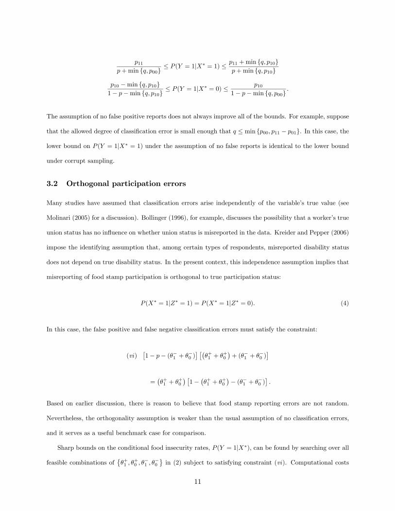
p11p+min fq; p00g

� P (Y = 1jX� = 1) � p11 +min fq; p10gp+min fq; p10g

p10 �min fq; p10g1� p�min fq; p10g

� P (Y = 1jX� = 0) � p101� p�min fq; p00g

.

The assumption of no false positive reports does not always improve all of the bounds. For example, suppose

that the allowed degree of classi�cation error is small enough that q � min fp00; p11 � p01g. In this case, the

lower bound on P (Y = 1jX� = 1) under the assumption of no false reports is identical to the lower bound

under corrupt sampling.

3.2 Orthogonal participation errors

Many studies have assumed that classi�cation errors arise independently of the variable�s true value (see

Molinari (2005) for a discussion). Bollinger (1996), for example, discusses the possibility that a worker�s true

union status has no in�uence on whether union status is misreported in the data. Kreider and Pepper (2006)

impose the identifying assumption that, among certain types of respondents, misreported disability status

does not depend on true disability status. In the present context, this independence assumption implies that

misreporting of food stamp participation is orthogonal to true participation status:

P (X� = 1jZ� = 1) = P (X� = 1jZ� = 0). (4)

In this case, the false positive and false negative classi�cation errors must satisfy the constraint:

(vi)�1� p� (��1 + ��0 )

� ���+1 + �

+0

�+ (��1 + �

�0 )�

=��+1 + �

+0

� �1�

��+1 + �

+0

�� (��1 + ��0 )

�.

Based on earlier discussion, there is reason to believe that food stamp reporting errors are not random.

Nevertheless, the orthogonality assumption is weaker than the usual assumption of no classi�cation errors,

and it serves as a useful benchmark case for comparison.

Sharp bounds on the conditional food insecurity rates, P (Y = 1jX�), can be found by searching over all

feasible combinations of��+1 ; �

+0 ; �

�1 ; �

�0

in (2) subject to satisfying constraint (vi). Computational costs

11

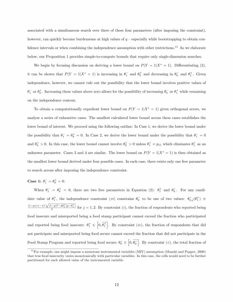
associated with a simultaneous search over three of these four parameters (after imposing the constraint),

however, can quickly become burdensome at high values of q �especially while bootstrapping to obtain con-

�dence intervals or when combining the independence assumption with other restrictions.12 As we elaborate

below, our Proposition 1 provides simple-to-compute bounds that require only single-dimension searches.

We begin by focusing discussion on deriving a lower bound on P (Y = 1jX� = 1). Di¤erentiating (2),

it can be shown that P (Y = 1jX� = 1) is increasing in ��1 and �+0 and decreasing in ��0 and �+1 . Given

independence, however, we cannot rule out the possibility that the lower bound involves positive values of

��1 or �+0 . Increasing these values above zero allows for the possibility of increasing �

�0 or �

+1 while remaining

on the independence contour.

To obtain a computationally expedient lower bound on P (Y = 1jX� = 1) given orthogonal errors, we

analyze a series of exhaustive cases. The smallest calculated lower bound across these cases establishes the

lower bound of interest. We proceed using the following outline: In Case 1, we derive the lower bound under

the possibility that ��1 = �+0 = 0. In Case 2, we derive the lower bound under the possibility that �

�1 = 0

and �+0 > 0. In this case, the lower bound cannot involve �+0 > 0 unless �

+1 = p11 which eliminates �

+1 as an

unknown parameter. Cases 3 and 4 are similar. The lower bound on P (Y = 1jX� = 1) is then obtained as

the smallest lower bound derived under four possible cases. In each case, there exists only one free parameter

to search across after imposing the independence constraint.

Case 1: ��1 = �+0 = 0:

When ��1 = �+0 = 0, there are two free parameters in Equation (2): �+1 and ��0 . For any candi-

date value of �+1 , the independence constraint (vi) constrains ��0 to be one of two values: ��0;j(�

+1 ) �

(1�p)+(�1)jp(1�p)2�4�+1 (p��

+1 )

2 for j = 1; 2. By constraint (i), the fraction of respondents who reported being

food insecure and misreported being a food stamp participant cannot exceed the fraction who participated

and reported being food insecure: �+1 2h0; �+1

i. By constraint (iv), the fraction of respondents that did

not participate and misreported being food secure cannot exceed the fraction that did not participate in the

Food Stamp Program and reported being food secure: ��0 2h0; ��0

i. By constraint (v), the total fraction of

12For example, one might impose a monotone instrumental variables (MIV) assumption (Manski and Pepper, 2000)that true food insecurity varies monotonically with particular variables. In this case, the cells would need to be furtherpartitioned for each allowed value of the instrumental variable.

12

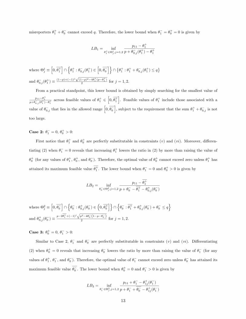
misreporters �+1 + ��0 cannot exceed q. Therefore, the lower bound when �

�1 = �

+0 = 0 is given by

LB1 = inf�+1 2�1

j ;j=1;2

p11 � �+1p+ ��0;j(�

+1 )� �+1

where �1j �h0; �+1

i\n�+1 : �

�0;j(�

+1 ) 2

h0; ��0

io\��+1 : �

+1 + �

�0;j(�

+1 ) � q

and ��0;j(�

+1 ) �

(1�p)+(�1)jp(1�p)2�4�+1 (p��

+1 )

2 for j = 1; 2.

From a practical standpoint, this lower bound is obtained by simply searching for the smallest value of

p11��+1p+��0;j(�

+1 )��

+1

across feasible values of �+1 2h0; �+1

i. Feasible values of �+1 include those associated with a

value of ��0;j that lies in the allowed rangeh0; ��0

i, subject to the requirement that the sum �+1 + �

�0;j is not

too large.

Case 2: ��1 = 0, �+0 > 0:

First notice that �+1 and �+0 are perfectly substitutable in constraints (v) and (vi). Moreover, di¤eren-

tiating (2) when ��1 = 0 reveals that increasing �+1 lowers the ratio in (2) by more than raising the value of

�+0 (for any values of �+1 , �

+0 , and �

�0 ). Therefore, the optimal value of �

+0 cannot exceed zero unless �

+1 has

attained its maximum feasible value �+1 . The lower bound when ��1 = 0 and �

+0 > 0 is given by

LB2 = inf��0 2�2

j ;j=1;2

p11 � �+1p+ ��0 � �+1 � �+0;j(�

�0 )

where �2j �h0; ��0

i\n��0 : �

+0;j(�

�0 ) 2

�0; �+0

io\n��0 : �

+1 + �

+0;j(�

�0 ) + �

�0 � q

oand �+0;j(�

�0 ) �

p�2�+1 +(�1)jqp2�4��0 (1�p��

�0 )

2 for j = 1; 2.

Case 3: �+0 = 0, ��1 > 0:

Similar to Case 2, ��1 and ��0 are perfectly substitutable in constraints (v) and (vi). Di¤erentiating

(2) when �+0 = 0 reveals that increasing ��0 lowers the ratio by more than raising the value of �

�1 (for any

values of �+1 , ��1 , and �

�0 ). Therefore, the optimal value of �

�1 cannot exceed zero unless �

�0 has attained its

maximum feasible value ��0 . The lower bound when �+0 = 0 and �

�1 > 0 is given by

LB3 = inf��1 2�3

j ;j=1;2

p11 + ��1 � �+1j(�

�1 )

p+ ��1 + ��0 � �+1j(�

�1 )

13

where �3j ��0; ��1

i\n��1 : �

+1j(�

�1 ) 2

h0; �+1

io\n��1 : �

�0 + �

+1j(�

�1 ) + �

�1 � q

oand �+1j(�

�1 ) �

p+(�1)jrp2�4

���0 +�

�1

��1�p���1 ��

�0

�2 for j = 1; 2.

Case 4: ��1 > 0, �+0 > 0:

Given �+1 = �+1 and �

�0 = �

�0 when �

�1 and �

+0 are positive, the lower bound when �

�1 > 0 and �

+0 > 0 is

given by

LB4 = inf�+0 2�4

j ;j=1;2

p11 + ��1j(�

+0 )� �+1

p+ ��1j(�+0 ) + �

�0 � �+1 � �+0

where �4j ��0; �+0

i\n�+0 : �

�1j(�

+0 ) 2

�0; ��1

io\n�+0 : �

+1 + �

�0 + �

�1j(�

+0 ) + �

+0 � q

oand ��1j(�

+0 ) �

1�p�2��0 +(�1)j

r(1�p)2�4

��+1 +�

+0

��p��+1 ��

+0

�2 for j = 1; 2.

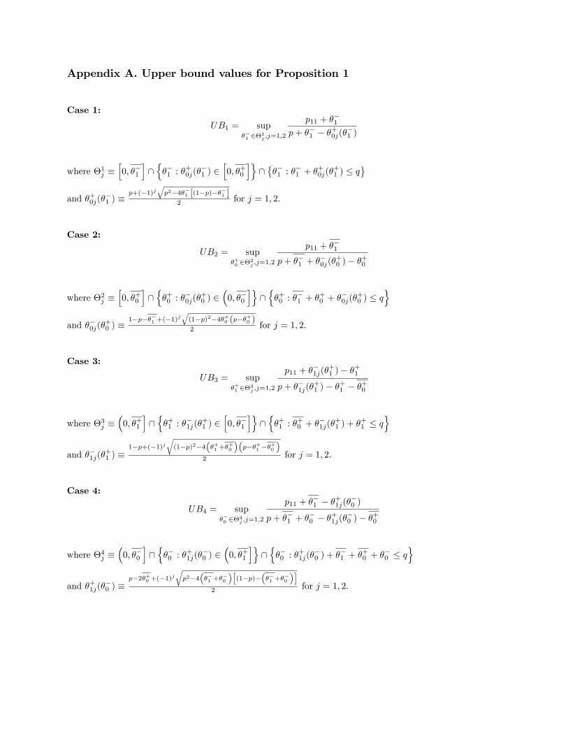
Combining these results with analogous results for upper bounds, we obtain the following proposition:

Proposition 1. Sharp bounds on P (Y = 1jX� = 1) under the orthogonal errors assumption in (4) are

identi�ed as

L � P (Y = 1jX� = 1) � H (5)

where L � inf fLB1; LB2; LB3; LB4g and H � sup fUB1; UB2; UB3; UB4g. Analogous bounds on P (Y =

1jX� = 0) are obtained by replacing X = 1 with X = 0, and vice versa, in the relevant quantities.

The expressions for the upper bounds are provided in Appendix A.13 The bounds converge to the self-

reported conditional food insecurity rate P (Y = 1jX = 1) as q goes to 0. Increasing q may widen the

bounds over some ranges of q but not others, and the rate of identi�cation decay can be highly nonlinear as

q increases.

These bounds are easy to program, and computing time is trivial given that searches are conducted in

a single dimension. To compute LB1, for example, we need only to search over feasible values of �+1 . In our

application, computational speed for the Proposition 1 bounds at q = 0:5 is more than 3300 times faster

than the speed associated with a simultaneous search across three of the four parameters �+1 , �+0 , �

�1 , and

13For su¢ ciently high values of q, some values lying between the worst-case lower and upper bounds may not befeasible under the independence constraint of Equation (4); sharp identi�cation regions can be constructed, if desired,by simply excluding such values.

14

��0 (reduced to three dimensions after incorporating the independence constraint).14 Moreover, the single-

dimensional search allows us to avoid specifying an arbitrary tolerance threshold for when independence is

satis�ed. If the speci�ed tolerance is too small, the calculated bounds become arti�cially narrow as feasible

bounds are excluded from consideration. In contrast, a large tolerance leads to unnecessarily conservative

estimated bounds. In practice, we found it quite time-consuming to �nd a reasonable balance between speed

and accuracy � a trade-o¤ that varies across di¤erent values of q. The proposed single-dimension search

procedure e¤ectively avoids this problem.

3.3 Food insecurity classi�cation errors

To this point, we have con�ned our attention to classi�cation errors in food stamp participation. For reasons

noted above, however, we might also suspect the presence of errors in food insecurity reports. Suppose that

true food insecurity status is measured by the latent indicator Y �. The observed indicator Y matches the

true value Y � if Z�0 = 1 and is misclassi�ed if Z�0 = 0. Analogous to the case of misreported food stamp

participation, let q0 represent an upper bound on the allowed degree of corruption in Y : P (Z�0 = 0) � q0.

Modifying Equation (1), the true food insecurity prevalence rate among food stamp recipients is given by

P (Y � = 1jX� = 1) =P (Y � = 1; X� = 1)

P (X� = 1). (6)

Given the possibility of classi�cation errors in both X and Y , there are now many more types of error

combinations. We represent these combinations by �uvjk . The subscripts j and k indicate true food insecurity

status and true food stamp participation status, respectively. Speci�cally, j = 1 indicates that the household

is truly food secure (j = 0 otherwise), and k = 1 indicates that the household truly receives food stamps

(k = 0 otherwise). The superscripts indicate whether these outcomes are falsely classi�ed, and if so, in

which direction. Speci�cally, u =�+�indicates that the household is misclassi�ed as food insecure, u =���

indicates that the household is misclassi�ed as food secure, and u =�o�indicates that food insecurity status

is not misclassi�ed. Similarly, v =�+� indicates that the household is misclassi�ed as receiving bene�ts,

v =��� indicates that the household is misclassi�ed as not receiving bene�ts, and v =�o� indicates that

participation status is not misclassi�ed.

14For di¤erent empirical applications, these values will vary depending on the quantities p11; p01; p10; p00 de�nedabove.

15

As before, we can decompose the numerator and denominator into observed and unobserved components:

P (Y � = 1jX� = 1) =P (Y = 1; X = 1) +

���o11 + �

o�11 + �

��11

����o+10 + �

+o01 + �

++00

�P (X = 1) +

��o�11 + �

��11 + �+�01 + �o�01

����o+10 + �

++00 + ��+10 + �o+00

� .Similarly, we can write

P (Y � = 1jX� = 0) =P (Y = 1; X = 0) +

���o10 + �

o+10 + �

�+10

����o�11 + �

+o00 + �

+�01

�P (X = 0) +

��o+10 + �

�+10 + �++00 + �o+00

����o�11 + �

+�01 + ���11 + �o�01

� .We can compute sharp bounds on P (Y � = 1jX�) by searching across all feasible combinations of false

positive and false negative classi�cations in X� and Y �. The following constraints must hold, analogous to

constraints (i -iv) earlier:

(i�) 0 � �+o01 ; �o+10 ; �++00 � P (Y = 1; X = 1) � p11

(ii�) 0 � �o+00 ; ��o11 ; ��+10 � P (Y = 0; X = 1) � p01

(iii�) 0 � �+o00 ; �o�11 ; �+�01 � P (Y = 1; X = 0) � p10

(iv�) 0 � ��o10 ; ���11 ; �o�01 � P (Y = 0; X = 0) � p00.

For example, the fraction of households simultaneously misclassi�ed as food insecure and misclassi�ed as

receiving food stamps, �++00 , cannot exceed the fraction of households who report being food insecure with

food stamps, p11. The errors must also satisfy the constraints

(v�) �o+00 + ��+10 + �o+10 + �

++00 + �o�11 + ���11 + �+�01 + �o�01 � q.

and

(v�) ��o11 + ��+10 + �+o01 + �

+o00 + �

++00 + �+�01 + ��o10 + �

��11 � q0:

A search over all combinations of errors becomes rapidly burdensome as the values of q and q0 are allowed

to rise. Nevertheless, the problem is feasible for su¢ ciently low degrees of potential data corruption. For

the case of corrupt sampling, the search problem is greatly simpli�ed because no structure is placed on

the pattern of errors. In that case, many of the unknown parameters for each bound can be set to 0. For

16

example, suppose we wish to compute a sharp lower bound on P (Y � = 1jX� = 1). It is easy to see that

the lower bound requires �o+00 = ��+10 = ��o11 = 0. Di¤erentiation further reveals that ���11 = �o�11 = 0 as

well. Analogous restrictions arise for the other bounds. For the case that we assume orthogonal errors in

X and/or Y , we cannot set any of the parameters to 0. Instead, we search over all feasible combinations

of errors subject to the requirement that candidates for the bounds are discarded unless the appropriate

orthogonality analogues to constraint (vi) are satis�ed.15

We next turn to empirical results. We �rst illustrate what can be identi�ed about conditional food

insecurity prevalence rates under the assumption that the receipt of bene�ts may be misclassi�ed but food

insecurity is accurately measured. We then allow for the possibility that food insecurity is misreported as

well. We pinpoint critical values of allowed degrees of data corruption for when we can no longer identify

that food stamp recipients are more likely to be food insecure than eligible nonrecipients.

4 Results

4.1 Food Stamp Classi�cation Errors

Figures 1 and 2 trace out patterns of identi�cation decay for inferences on the prevalence of food insecurity

among food stamp recipients and nonrecipients, respectively, as a function of the allowed degree of data

corruption, q. As discussed above, we focus our attention on eligible households with children. For these

�gures, we assume that only food stamp participation is subject to classi�cation error; food insecurity

classi�cations are presumed to be accurate.

In Figure 1 we examine what can be known about P (Y � = 1jX � = 1), the prevalence of food insecurity

among food stamp recipients. When q = 0, all food stamp classi�cations are taken at face value; uncertainty

about the magnitude of � arises from sampling variability alone. As seen in Figure 1 and the table beneath

it, the prevalence rate at q = 0 is point-identi�ed as p11 = 0:523 with 90% con�dence interval [0:496; 0:545].

What can be known about P (Y � = 1jX� = 1) when q > 0 depends on what the researcher is willing

to assume about the nature and degree of reporting errors. First suppose nothing is known about the

pattern of reporting errors. If q = 0:05, then up to 5% of the food stamp classi�cations may be inaccurate.

In this case, P (Y � = 1jX � = 1) is partially identi�ed to lie within the range [0:457; 0:595], a 14 point

15Our Gauss computer code for computing these bounds is available upon request.

17

range. After accounting for sampling variability, this range expands to [0:427; 0:621], a 19 point range.

The �gure traces out the 5th percentile lower bound and 95th percentile upper bound across values of q.16

The bounds naturally widen as our con�dence in the reliability of the data declines. When q rises to 0:10,

P (Y � = 1jX� = 1) is bounded to lie within [0:370; 0:691], a 32 point range, before accounting for sampling

variability. Once q exceeds about 0:21, we cannot say anything about the food insecurity rate of food stamp

recipients; the prevalence rate could lie anywhere within [0; 1].

The bounds narrow if we are willing to make assumptions about the pattern of errors. If classi�ca-

tion errors do not depend on true participation status (Orthogonal Errors), then the bounds narrow to

[0:461; 0:586] (before accounting for sampling variability) at q = 0:05 and to [0:396; 0:652] at q = 0:10. If

we instead assume away the possibility of false positive food stamp reports (No False Positives), the bounds

narrow yet further to [0:466; 0:575] and [0:421; 0:616]. In this case, these assumptions restricting the nature

of reporting errors improve the lower and upper bounds in about the same proportions.

Figure 2 presents analogous bounds for P (Y � = 1jX � = 0), the prevalence of food insecurity among

nonrecipients. At q = 0, this prevalence rate is point-identi�ed as p10 = 0:344, about 18 points lower than

the food insecurity rate among recipients. For q > 0, the orthogonality restriction substantially improves the

lower bound relative to corrupt sampling. The upper bound, however, is not substantially improved except

for high values of q. The assumption of no false positive classi�cations marginally improves the upper bound

and has no e¤ect on the lower bound.

Figure 3 provides sharp bounds on � � P (Y � = 1jX � = 1)�P (Y � = 1jX � = 0), the di¤erence in food

insecurity rates (Figure 3A) and food insecurity with hunger rates (Figure 3B) between food stamp recipients

and nonrecipients. A simple lower (upper) bound on � could be computed as the di¤erence between the

lower (upper) bound on P (Y � = 1jX� = 1) and the upper (lower) bound on P (Y � = 1jX� = 0). Such bounds

would not as tight as possible, however, because a di¤erent set of values of��+1 ; �

+0 ; �

�1 ; �

�0

might maximize

(minimize) the expression in Equation (2) than would minimize (maximize) the expression in Equation (3).

16We bootstrap to obtain these values using the bias-corrected percentile method (Efron and Tibshirani, 1993)using 1,000 pseudosamples. The kinks at various values of q re�ect the impacts of constraints (i)-(vi) on allowedcombinations of false positives and false negatives (Section 3). For su¢ ciently small values of q, constraints (i)-(iv )are not binding because constraint (vi) prevents �+1 ; �

+0 ; �

�1 ; or �

�0 from attaining their maximum feasible values. As

q rises, however, each of the other constraints eventually becomes binding, resulting in a kink in the �gure. This kinkis somewhat smoothed by bootstrapping across the pseudosamples.

18

Instead, we obtain sharp bounds on � as follows:

�LB = min�+1 ;�

+0 ;�

�1 ;�

�0

(p11 + �

�1 � �+1

p+���1 + �

�0

����+1 + �

+0

� � p10 + �+1 � ��1

1� p+��+1 + �

+0

�����1 + �

�0

�)

�UB = max�+1 ;�

+0 ;�

�1 ;�

�0

(p11 + �

�1 � �+1

p+���1 + �

�0

����+1 + �

+0

� � p10 + �+1 � ��1

1� p+��+1 + �

+0

�����1 + �

�0

�)

subject to all constraints imposed on the pattern of classi�cation errors.

Figure 3A shows that small degrees of classi�cation error are su¢ cient to overturn the conclusion from

the data that � > 0, even without accounting for uncertainty arising from sampling variability. Under

corrupt sampling, we cannot identify that � is positive if more than 7:1% of households might misreport

their food stamp participation status. Under orthogonal errors, this critical value rises to 8:2%. Even under

the assumption of no false positive classi�cations, identi�cation deteriorates rapidly enough that we cannot

rule out the possibility that � is negative if food stamps participation is underreported by more than 9:1%

of the sample.

Panel B in the �gure reproduces Panel A except that Y � = 1 is rede�ned as food insecurity with hunger.

Here, we �nd that identi�cation of the sign of � breaks down when q is only 0:018 under corrupt sampling

and when q is only 0:029 under orthogonal errors. Both of these are far lower than in the case of food

insecurity. When the presence of false positive participation reports is assumed away, the critical value of q

rises to 0:124 which is higher than for food insecurity. Again, these critical values are conservatively high in

that they do not account for the additional uncertainty created by sampling variability.17

As discussed in Section 2.2, Bollinger and David (1997) �nd that 12% of households fail to report their

receipt of food stamps; evidence from Bitler et al. (2003) suggests the possibility of even greater degrees

of undercounting. Thus, even before accounting for the possible mismeasurement of food insecurity status,

we �nd it di¢ cult to conclude that food insecurity is more prevalent among food stamp recipients than

among eligible nonrecipients. Such a conclusion requires a large degree of con�dence in self-reported food

participation status. In the next section, we extend the analysis to the case that both food stamp recipiency

and food insecurity may be misclassi�ed.

17Appendix Figures 1 and 2 depict bounds on the conditional food insecurity with hunger prevalence rates, P (Y � =1jX� = 1) and P (Y � = 1jX� = 0), respectively.

19

4.2 Food stamp and food insecurity classi�cation errors

As discussed above, the possibility of classi�cation errors in food insecurity status further confounds identi-

�cation of the parameters of interest. Table 2 provides critical values for identi�cation breakdown that vary

across di¤erent assumptions on the nature of classi�cation errors. Row A reproduces information highlighted

in Figure 3A for the case of perfectly accurate food insecurity classi�cations. For the case of arbitrarily mis-

reported food stamp recipiency in Column (i), the sign of � is identi�ed to be positive unless more than

7:1% of households might misreport food stamp participation. These values rise to 8:2% and 9:1% for the

cases of orthogonal errors and no false positive reports, respectively.

Now suppose that food insecurity status might be misclassi�ed for up to 5% of households: q0 = 0:05.

If potential food insecurity classi�cation errors arise independently of true food insecurity status (Row B),

then the sign of � cannot be identi�ed under arbitrary program participation errors unless it is assumed that

fewer than 2:8% of households might misreport their food stamp recipiency. These critical values rise only

slightly under the stronger assumptions of orthogonal food stamp errors (3:3%) and no false positive food

stamp reports (4:1%). In Row C for the case of arbitrarily misreported food insecurity status, the critical

values fall further to 2:1%, 2:4%, and 3:5%, respectively.

When Y � = 1 is de�ned to classify food insecurity with hunger, yet smaller degrees of uncertainty

about the data are su¢ cient to lose identi�cation of the sign of �. Even assuming away the existence of

classi�cation errors in food stamp recipiency (i.e., q = 0) and supposing that errors in Y � arise independently

of the variable�s true value, the sign of� is not identi�ed unless q0 < 0:028 �an error rate of less than 3%. This

critical value is conservatively large in that we have abstracted away from sampling variability. Collectively,

these �ndings suggest that we should not be con�dent that food stamp recipient households are less likely to

be food secure than nonrecipient households unless we are willing to place a very large degree of con�dence

in the responses.

5 Conclusion

As the cornerstone of the federal food assistance system, the Food Stamp Program is charged with being

the �rst line of defense against hunger. In this light, researchers and policymakers have been puzzled to

observe negative relationships between food security and the receipt of food stamps among observationally

20

similar eligible households. We �nd that this paradox, however, hinges critically on an assumption of

accurate classi�cations. Food insecurity responses are partially subjective, and evidence from Bollinger and

David (1997) suggests that error rates in self-reported food stamp recipiency exceed 12%. We introduced

a nonparametric empirical framework for assessing what can be inferred about conditional probabilities

when a binary outcome and conditioning variable are both subject to nonclassical measurement error. We

�nd that food stamp participation error rates much smaller than 12% are su¢ cient to overturn prevailing

conclusions, even under strong assumptions restricting the patterns of errors. The possibility of misreported

food insecurity exacerbates the uncertainty.

More generally, our analysis derives easy-to-compute sharp bounds on partially identi�ed conditional

probabilities in the presence of arbitrary endogenous classi�cation errors. The framework can be applied

to a wide range of topics in the social sciences involving nonrandom classi�cation errors. We have not,

however, attempted to provide a structural model of food stamp eligibility and participation. Our approach,

for example, cannot identify the policy impacts of proposed changes in food assistance programs. Instead,

our approach is intended to provide a useful starting point for understanding what can be known about

relationships between food insecurity and food stamp participation under current policies. We hope that

future research aimed at identifying food assistance policy e¤ects will explicitly account for the uncertainty

associated with potential reporting errors in the key variables of interest.

21

References

[1] Aigner, D. (1973). �Regression with a Binary Independent Variable subject to Errors of Observations.�

Journal of Econometrics, 1, 49-60.

[2] Barron, J., D. Black, and M. Berger. (1997). �Employer Search, Training, and Vacancy Duration,�

Economic Inquiry, 35(1), 167-92.

[3] Berger, M., Black, D., Scott, F. (2000). �Bounding Parameter Estimates With Non-classical Measure-

ment Error.�Journal of the American Statistical Association, 95: 739�748.

[4] Berger M., D. Black, and F. Scott. (1998). �How Well Do We Measure Employer-Provided Health

Insurance Coverage?�Contemporary Economic Policy, 16: 356-67.

[5] Bhattacharya, J., J. Currie, and S. Haider. (2004). �Poverty, Food Insecurity, and Nutritional Outcomes

in Children and Adults.�Journal of Health Economics, 23(4): 839-62.

[6] Bitler, M., J. Currie, and J.K. Scholz. (2003). �WIC Eligibility and Participation,�Journal of Human

Resources, 38(S): 1139-1179.

[7] Bitler, M., C. Gundersen, and G. Marquis. (2005). �Are WIC Non-Recipients at Less Nutritional Risk

than Recipients? An Application of the Food Security Measure.�Review of Agricultural Economics,

27(3): 433�38.

[8] Black, D., S. Sanders, and L. Taylor. (2003). �Measurement of Higher Education in the Census and

CPS,�Journal of the American Statistical Association, 98 (463), 545-54.

[9] Bollinger, C. (1996). �Bounding Mean Regressions When a Binary Regressor is Mismeasured.�Journal

of Econometrics, 73: 387-99.

[10] Bollinger, C. and M. David. (1997). �Modeling Discrete Choice with Response Error: Food Stamp

Participation.�Journal of the American Statistical Association, 92:827-35.

[11] Bollinger, C. and M. David. (2001). �Estimation With Response Error and Nonresponse: Food Stamp

Participation in the SIPP.�Journal of Business and Economic Statistics, 19: 129-142.

[12] Bollinger, C. and M. David. (2005). �I Didn�t Tell, and I Won�t Tell: Dynamic Response Error in the

SIPP.�Journal of Applied Econometrics, 20: 563-569.

[13] Borjas, G. (2004). �Food Insecurity and Public Assistance.�Journal of Public Economics, 88: 1421-43.

[14] Bound, J. (1991). �Self-Reported Versus Objective Measures of Health in Retirement Models.�Journal

of Human Resources, 36: 106-38.

[15] Bound, J. and Burkhauser, R. (1999). �Economic Analysis of Transfer Programs Targeted on People

with Disabilities.�In Orley Ashenfelter and David Card (Eds.), Handbook of Labor Economics, Vol. 3C.

Amsterdam: Elsevier Science, 3417-3528.

[16] Cunnyngham, K. and B. Brown. (2004). Characteristics of Food Stamp Households: Fiscal Year 2003.

U.S. Department of Agriculture, Food and Nutrition Service.

[17] Cunnyngham, K. (2005). Food Stamp Program participation rates: 2003. Washington DC: U.S. De-

partment of Agriculture, Food and Nutrition Service.

[18] Dominitz, J., and R. Sherman. (2004). �Sharp Bounds Under Contaminated or Corrupted Sampling

With Veri�cation, With an Application to Environmental Pollutant Data,� Journal of Agricultural,

Biological and Environmental Statistics, 9(3), 319-38.

[19] Dunifon, R., and L. Kowaleski-Jones. (2003). �The In�uences of Participation in the National School

Lunch Program and Food Insecurity on Child Well-Being.�Social Service Review, 77(1): 72-92.

[20] Efron, B., and R. Tibshirani. (1993). An Introduction to the Bootstrap. London: Chapman and Hall.

[21] Frazis, H. and M. Loewenstein. (2003). �Estimating Linear Regressions with Mismeasured, Possibly

Endogenous, Binary Explanatory Variables,�Journal of Econometrics, 117, 151-78.

[22] Furness, B., P. Simon, C. Wold, and J. Asarian-Anderson. (2004). �Prevalence and Predictors of Food

Insecurity Among Low-Income Households in Los Angeles County.�Public Health Nutrition, 7(6): 791-4.

[23] Ginther, D. (2000). �Alternative Estimates of the E¤ect of Schooling on Earnings.�Review of Economics

and Statistics 82: 103-116.

[24] Gundersen, C. and S. O¤utt. (2005). �Farm Poverty and Safety Nets.�American Journal of Agricultural

Economics, 87(4), 885�99.

[25] Gundersen, C. and V. Oliveira. (2001). �The Food Stamp Program and Food Insu¢ ciency.�American

Journal of Agricultural Economics, 83(4): 875-87.

[26] Gundersen, C. and D. Ribar. (2005). �Food Insecurity and Insu¢ ciency at Low Levels of Food Expen-

ditures.�Institute for the Study of Labor (IZA) Working Paper No. 1594.

[27] Gundersen, C., L. Weinreb, C. Wehler, and D. Hosmer. (2003). �Homelessness and Food Insecurity.�

Journal of Housing Economics, 12(3): 250-72.

[28] Haider, S., A. Jacknowitz, and R. Schoeni. (2003). �Food Stamps and the Elderly: Why is Participation

So Low?�Journal of Human Resources, 38: 1080-1111.

[29] Hamelin, A., M. Beaudry, and J. Habicht. (2002). �Characterization of Household Food Insecurity in

Quebec: Food and Feelings�Social Science and Medicine, 54: 119-32.

[30] Hausman, J.A., J. Abrevaya, and F.M. Scott-Morton. (1998). �Misclassi�cation of the Dependent Vari-

able in a Discrete-Response Setting.�Journal of Econometrics, 87: 239-69.

[31] Horowitz, J. and C. Manski. (1995). �Identi�cation and Robustness With Contaminated and Corrupted

Data.�Econometrica 63: 281-302.

[32] Huber, P. (1981), Robust Statistics, New York: Wiley.

[33] Kreider, B. and J. Pepper. (forthcoming). �Disability and Employment: Reevaluating the Evidence in

Light of Reporting Errors.�Journal of the American Statistical Association.

[34] and . (2006). �Inferring Disability Status from Corrupt Data.�Working Paper. Iowa State

University.

[35] Laraia, B., A. Siega-Riz, C. Gundersen, and N. Dole. (2006). �Psychosocial factors and socioeconomic

indicators are associated with household food insecurity among pregnant women,�Journal of Nutrition,

136: 177�182.

[36] Manski, C. (2003). Partial Identi�cation of Probability Distributions, Springer Series in Statistics, New

York.

[37] Marquis, K. and J. Moore. (1990). �Measurement errors in SIPP program reports�in Proceedings of the

Bureau of the Census Annual Research Conference, Washington, DC: Bureau of the Census, 721-745.

[38] Mo¢ tt, R. (1983). �An Economic Model of Welfare Stigma.�American Economic Review, 73: 1023-35.

[39] Molinari, F. (2005). �Partial Identi�cation of Probability Distributions with Misclassi�ed Data.�Work-

ing Paper. Department of Economics, Cornell University.

[40] National Research Council. (2006). Food Insecurity and Hunger: An Assessment of the Measure. G.

Wunderlich and J. Norwood (eds.). Washington, DC: The National Academies Press.

[41] Nord, M., M. Andrews, and S. Carlson. (2004). Household Food Security in the United States, 2003,

Washington, DC: U.S. Department of Agriculture, Economic Research Service, Food Assistance and

Nutrition Research Report 42.

[42] Nord, M., M. Andrews, and S. Carlson. (2005). Household Food Security in the United States, 2004,

Washington, DC: U.S. Department of Agriculture, Economic Research Service, Economic Research

Report No. 11.

[43] Pepper, J. (2000). �The Intergenerational Transmission of Welfare Receipt: A Nonparametric Bounds

Analysis,�Review of Economics and Statistics, 82(3), 472-288.

[44] Ranney, C. and J. Kushman. (1987). �Cash Equivalence, Welfare Stigma, and Food Stamps.�Southern

Economic Journal, 53: 1011-27.

[45] Ribar, D. and K. Hamrick. (2003). Dynamics of Poverty and Food Su¢ ciency, Washington, DC: U.S.

Department of Agriculture, Economic Research Service, Food Assistance and Nutrition Research Report

33.

[46] Trippe, G. P. Doyle, and A. Asher. (1992). Trends in Food Stamp Program Participation Rates: 1976

to 1009. Current Perspectives on Food Stamp Participation, Washington DC: U.S. Department of Agri-

culture, Food and Nutrition Service.

[47] U.S. Department of Agriculture (1999). Food and Nutrition Service. Annual Historical Review: Fiscal

year 1997.

[48] Van Hook J., and K. Balistreri. (2006). �Ineligible Parents, Eligible Children: Food Stamps Receipt,

Allotments, and Food Insecurity Among Children of Immigrants.�Social Science Research, 35, 228-51.

[49] Vozoris, N. and V. Tarasuk. (2003). �Household Food Insu¢ ciency is Associated with Poorer Health.�

Journal of Nutrition, 133, 120-26.

Appendix A. Upper bound values for Proposition 1

Case 1:

UB1 = sup��1 2�1

j ;j=1;2

p11 + ��1

p+ ��1 � �+0j(��1 )

where �1j �h0; ��1

i\n��1 : �

+0j(�

�1 ) 2

h0; �+0

io\���1 : �

�1 + �

+0j(�

+1 ) � q

and �+0j(�

�1 ) �

p+(�1)jqp2�4��1 [(1�p)��

�1 ]

2 for j = 1; 2.

Case 2:

UB2 = sup�+0 2�2

j ;j=1;2

p11 + ��1

p+ ��1 + ��0j(�

+0 )� �+0

where �2j �h0; �+0

i\n�+0 : �

�0j(�

+0 ) 2

�0; ��0

io\n�+0 : �

�1 + �

+0 + �

�0j(�

+0 ) � q

oand ��0j(�

+0 ) �

1�p���1 +(�1)jq(1�p)2�4�+0 (p��

+0 )

2 for j = 1; 2.

Case 3:

UB3 = sup�+1 2�3

j ;j=1;2

p11 + ��1j(�

+1 )� �+1

p+ ��1j(�+1 )� �+1 � �+0

where �3j ��0; �+1

i\n�+1 : �

�1j(�

+1 ) 2

h0; ��1

io\n�+1 : �

+0 + �

�1j(�

+1 ) + �

+1 � q

oand ��1j(�

+1 ) �

1�p+(�1)jr(1�p)2�4

��+1 +�

+0

��p��+1 ��

+0

�2 for j = 1; 2.

Case 4:

UB4 = sup��0 2�4

j ;j=1;2

p11 + ��1 � �+1j(�

�0 )

p+ ��1 + ��0 � �+1j(�

�0 )� �+0

where �4j ��0; ��0

i\n��0 : �

+1j(�

�0 ) 2

�0; �+1

io\n��0 : �

+1j(�

�0 ) + �

�1 + �

+0 + �

�0 � q

oand �+1j(�

�0 ) �

p�2�+0 +(�1)j

rp2�4

���1 +�

�0

�h(1�p)�

���1 +�

�0

�i2 for j = 1; 2.

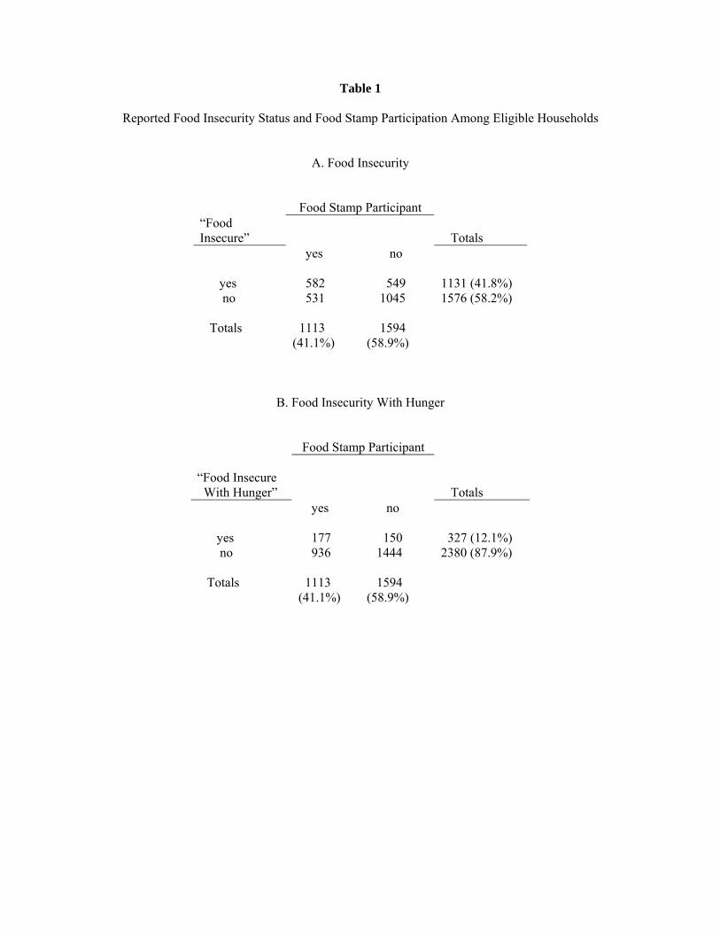
Table 1

Reported Food Insecurity Status and Food Stamp Participation Among Eligible Households

A. Food Insecurity

Food Stamp Participant “Food Insecure”

Totals

yes no yes 582 549 1131 (41.8%) no 531 1045 1576 (58.2%) Totals 1113 1594 (41.1%) (58.9%)

B. Food Insecurity With Hunger

Food Stamp Participant “Food Insecure With Hunger”

Totals

yes no yes 177 150 327 (12.1%) no 936 1444 2380 (87.9%) Totals 1113 1594 (41.1%) (58.9%)

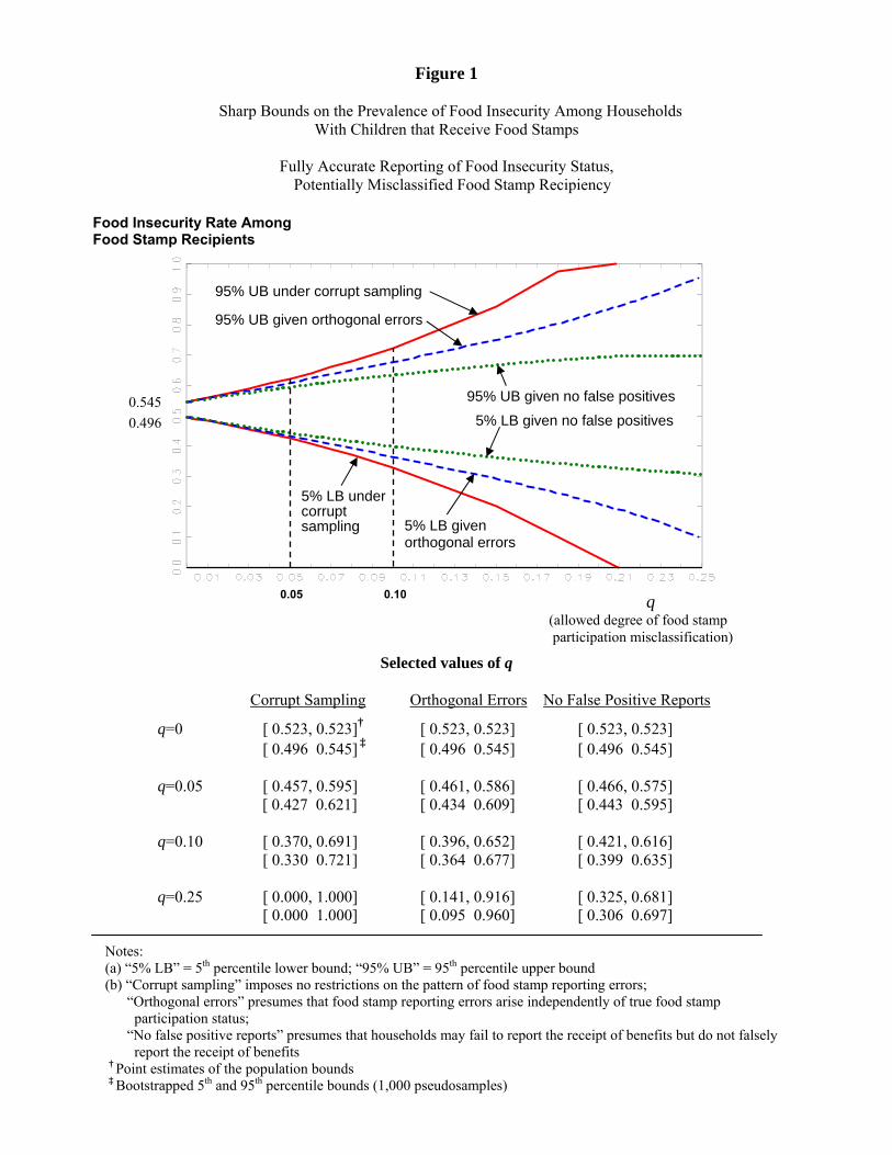
Figure 1

Sharp Bounds on the Prevalence of Food Insecurity Among Households With Children that Receive Food Stamps

Fully Accurate Reporting of Food Insecurity Status, Potentially Misclassified Food Stamp Recipiency

Food Insecurity Rate Among Food Stamp Recipients

95% UB under corrupt sampling

95% UB given orthogonal errors

5% LB undercorrupt sampling

5% LB given no false positives

95% UB given no false positives 0.545

0.496

5% LB given

orthogonal errors 0.05 0.10 q

(allowed degree of food stamp participation misclassification)

Selected values of q

Corrupt Sampling Orthogonal Errors No False Positive Reports

q=0 [ 0.523, 0.523]† [ 0.523, 0.523] [ 0.523, 0.523] [ 0.496 0.545] ‡ [ 0.496 0.545] [ 0.496 0.545]

q=0.05 [ 0.457, 0.595] [ 0.461, 0.586] [ 0.466, 0.575] [ 0.427 0.621] [ 0.434 0.609] [ 0.443 0.595]

q=0.10 [ 0.370, 0.691] [ 0.396, 0.652] [ 0.421, 0.616]

[ 0.330 0.721] [ 0.364 0.677] [ 0.399 0.635]

q=0.25 [ 0.000, 1.000] [ 0.141, 0.916] [ 0.325, 0.681] [ 0.000 1.000] [ 0.095 0.960] [ 0.306 0.697]

Notes: (a) “5% LB” = 5th percentile lower bound; “95% UB” = 95th percentile upper bound (b) “Corrupt sampling” imposes no restrictions on the pattern of food stamp reporting errors; “Orthogonal errors” presumes that food stamp reporting errors arise independently of true food stamp participation status; “No false positive reports” presumes that households may fail to report the receipt of benefits but do not falsely report the receipt of benefits † Point estimates of the population bounds ‡ Bootstrapped 5th and 95th percentile bounds (1,000 pseudosamples)

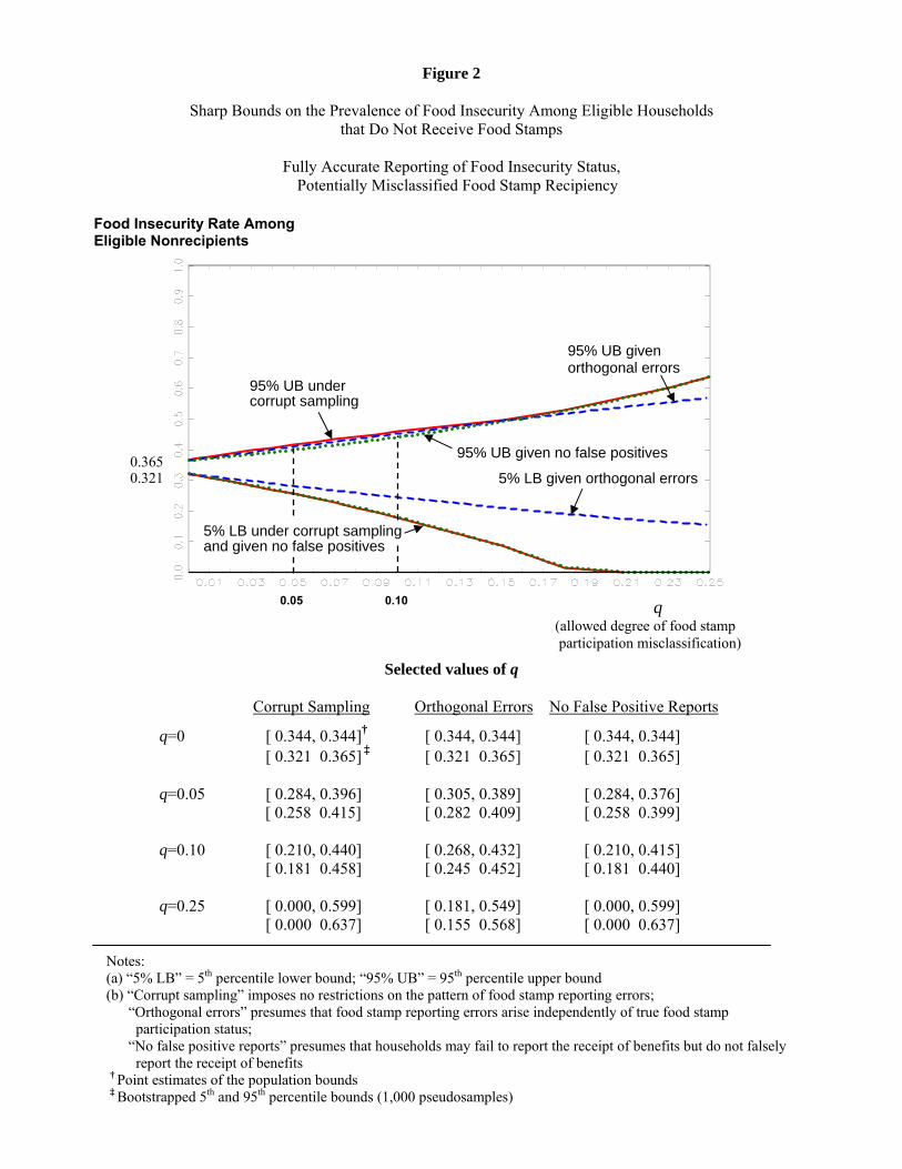
Figure 2

Sharp Bounds on the Prevalence of Food Insecurity Among Eligible Households that Do Not Receive Food Stamps

Fully Accurate Reporting of Food Insecurity Status, Potentially Misclassified Food Stamp Recipiency

Food Insecurity Rate Among Eligible Nonrecipients

95% UB given orthogonal errors

95% UB under corrupt sampling

95% UB given no false positives

0.365 0.321 5% LB given orthogonal errors

5% LB under corrupt sampling

and given no false positives 0.05 0.10 q

(allowed degree of food stamp participation misclassification)

Selected values of q

Corrupt Sampling Orthogonal Errors No False Positive Reports

q=0 [ 0.344, 0.344]† [ 0.344, 0.344] [ 0.344, 0.344] [ 0.321 0.365] ‡ [ 0.321 0.365] [ 0.321 0.365]

q=0.05 [ 0.284, 0.396] [ 0.305, 0.389] [ 0.284, 0.376] [ 0.258 0.415] [ 0.282 0.409] [ 0.258 0.399]

q=0.10 [ 0.210, 0.440] [ 0.268, 0.432] [ 0.210, 0.415]

[ 0.181 0.458] [ 0.245 0.452] [ 0.181 0.440]

q=0.25 [ 0.000, 0.599] [ 0.181, 0.549] [ 0.000, 0.599] [ 0.000 0.637] [ 0.155 0.568] [ 0.000 0.637]

Notes: (a) “5% LB” = 5th percentile lower bound; “95% UB” = 95th percentile upper bound (b) “Corrupt sampling” imposes no restrictions on the pattern of food stamp reporting errors; “Orthogonal errors” presumes that food stamp reporting errors arise independently of true food stamp participation status; “No false positive reports” presumes that households may fail to report the receipt of benefits but do not falsely report the receipt of benefits † Point estimates of the population bounds ‡ Bootstrapped 5th and 95th percentile bounds (1,000 pseudosamples)

Figure 3

Sharp Bounds on the Difference in Food Insecurity Prevalence Rates Between Food Stamp Recipients and Nonrecipients (Among Eligible Households with Children)

Fully Accurate Reporting of Food Insecurity Status,

Potentially Misclassified Food Stamp Recipiency

A. Food Insecurity 0.178

B. Food Insecurity with Hunger

Difference in Food Insecurity With Hunger Prevalence Rates (Δ)

Difference in Food Insecurity Prevalence Rates (Δ)

† Point estimates of the population bounds

0.064

UB undercorrupt sampling

UB given orthogonal errors UB given

no false positives

LB given orthogonal errors LB given no false

positives

LB under corrupt sampling

0.018 0.029

LB under corrupt sampling LB given no false

positives LB given orthogonal errors

UB under corrupt sampling

0.071 0.082 0.101

0.124

UB given no false positives

UB given orthogonal errors

q

q

Table 2

Critical Values for the Maximum Allowed Degree of Food Stamp Recipiency Misclassification Before the Sign of the Food Insecurity Gap, Δ, is No Longer Identified

Type of Classification Error in Food Stamp Participation Status, X*

Type of Classification Error in Food Insecurity Status, Y* (i) Arbitrary errors

(corrupt sampling) (ii) Orthogonal errors: P(X*=1|Z’) = P(X*=1) (iii) No False Positive

Classifications

Critical value of q:† Critical value of q: Critical value of q: A. No food insecurity classification errors 0.071 0.082 0.101 B. Orthogonal errors: P(Y*=1|Z’) = P(Y*=1) with q’ = 0.05

0.028 0.033 0.041

C. Arbitrary errors (corrupt sampling) with q’ = 0.05

0.021 0.024 0.035

†Maximum allowed degree of reporting error in food stamp participation, qc, such that the sign of Δ is no longer identified for higher allowed error rates. Note: All critical values are conservatively large in that they are calculated based on point estimates of the bounds on Δ (instead of using 5th percentile lower bounds as depicted in the figures). Critical values that account for the additional uncertainty associated with sampling variability would be smaller. Bootstrapping computational costs are prohibitively large when allowing for classification errors in both X* and Y*.

Appendix Figure 1

Sharp Bounds on the Prevalence of Food Insecurity With Hunger Among Households With Children that Receive Food Stamps

Fully Accurate Reporting of Food Insecurity With Hunger Status,

Potentially Misclassified Food Stamp Recipiency

Food Insecurity Rate Among Food Stamp Recipients

95% UB given

orthogonal errors

0.545 5% and 95% bounds under corrupt sampling

0.496

5% LB given no false positives 95% UB given no false positives

5% LB given orthogonal errors 0.05 0.10 q

(allowed degree of food stamp participation misclassification)

Selected values of q

Corrupt Sampling Orthogonal Errors No False Positive Reports

q=0 [ 0.159, 0.159]† [ 0.159, 0.159] [ 0.159, 0.159] [ 0.142 0.177] ‡ [ 0.142 0.177] [ 0.142 0.177]

q=0.05 [ 0.043, 0.250] [ 0.088, 0.213] [ 0.142, 0.250] [ 0.026 0.265] [ 0.074 0.231] [ 0.127 0.265]

q=0.10 [ 0.000, 0.286] [ 0.011, 0.268] [ 0.128, 0.259]

[ 0.000 0.304] [ 0.000 0.286] [ 0.114 0.277]

q=0.25 [ 0.000, 0.444] [ 0.000, 0.375] [ 0.099, 0.259] [ 0.000 0.475] [ 0.000 0.420] [ 0.089 0.277]

Notes: (a) “5% LB” = 5th percentile lower bound; “95% UB” = 95th percentile upper bound (b) “Corrupt sampling” imposes no restrictions on the pattern of food stamp reporting errors; “Orthogonal errors” presumes that food stamp reporting errors arise independently of true food stamp participation status; “No false positive reports” presumes that households may fail to report the receipt of benefits but do not falsely report the receipt of benefits † Point estimates of the population bounds ‡ Bootstrapped 5th and 95th percentile bounds (1,000 pseudosamples)

Appendix Figure 2

Sharp Bounds on the Prevalence of Food Insecurity With Hunger Among Eligible Households that Do Not Receive Food Stamps

Fully Accurate Reporting of Food Insecurity Status, Potentially Misclassified Food Stamp Recipiency

Food Insecurity Rate Among Eligible Nonrecipients

95% UB given

orthogonal errors

95% UB undercorrupt sampling

5% LB under corrupt sampling and under no false positives

95% UB given no false positives

0.365 0.321

5% LB given orthogonal errors

0.05 0.10 q

(allowed degree of food stamp participation misclassification)

Selected values of q

Corrupt Sampling Orthogonal Errors No False Positive Reports

q=0 [ 0.094, 0.094]† [ 0.094, 0.094] [ 0.094, 0.094] [ 0.083 0.105] ‡ [ 0.083 0.105] [ 0.083 0.105]

q=0.05 [ 0.010, 0.165] [ 0.059, 0.142] [ 0.010, 0.103] [ 0.000 0.175] [ 0.048 0.154] [ 0.000 0.115]

q=0.10 [ 0.000, 0.195] [ 0.027, 0.191] [ 0.000, 0.113]

[ 0.000 0.206] [ 0.015 0.200] [ 0.000 0.127]

q=0.25 [ 0.000, 0.257] [ 0.000, 0.197] [ 0.000, 0.164] [ 0.000 0.271] [ 0.000 0.212] [ 0.000 0.182]

Notes: (a) “5% LB” = 5th percentile lower bound; “95% UB” = 95th percentile upper bound (b) “Corrupt sampling” imposes no restrictions on the pattern of food stamp reporting errors; “Orthogonal errors” presumes that food stamp reporting errors arise independently of true food stamp participation status; “No false positive reports” presumes that households may fail to report the receipt of benefits but do not falsely report the receipt of benefits † Point estimates of the population bounds ‡ Bootstrapped 5th and 95th percentile bounds (1,000 pseudosamples)