Formation of cyclotron–annihilation lines in magnetized vacuum near neutron stars

Mon. Not. R. Astron. Soc. 368, 976–984 (2006) doi:10.1111/j.1365-2966.2006.10176.x

Formation of cyclotron–annihilation lines in magnetized vacuum nearneutron stars

V. A. Kukushkin�

Institute of Applied Physics of the RAS, 46 Ulyanov Street, Nizhny Novgorod 603950, Russia

Accepted 2006 February 8. Received 2006 February 8; in original form 2005 September 19

ABSTRACT

We study the formation of the absorption features, called the cyclotron–annihilation lines, inthe γ -spectra of the neutron stars (pulsars), owing to the fundamental quantum-electrodynamiceffect of the one–photon pair creation in magnetized vacuum. As a result, we substantiate anew method for the determination of the neutron star magnetic fields B based on measuring theinterval between the main annihilation and the first cyclotron–annihilation absorption lines.It is found that these lines may be easily resolved, and, consequently, the method is surelyapplicable if the following conditions are satisfied. (i) A γ -source has to be compact enoughand located near a star, but not close to its magnetic poles. For instance, it may be a disc inthe plane of a star magnetic equator with latitudinal angular width less than

√B/4.4 × 1013 G

and radial extent up to 25 per cent of the star radius. (ii) The source is to produce detectableγ -radiation at large angles �60◦ to the local magnetic field. Being situated in a closedfield line region and having a broad radiation pattern, such a source is not what is usuallyconsidered in the context of the polar cap and outer gap models of the pulsar γ -emissiondealing with open field lines only. (iii) Magnetic field strength must lie in a certain nar-row interval with the centre at ∼(3–4) × 1012 G. Its width depends on the star orientationand disc radial extend and in the most favourable case is about 20–30 per cent of its lowerboundary. Finally, the influence of the star rotation on this method employment is consid-ered and new possibilities arising from forthcoming polarization observations are brieflydiscussed.

Key words: line: formation – stars: magnetic fields – stars: neutron – gamma-rays: theory.

1 I N T RO D U C T I O N

A reliable and accurate determination of the magnetic field strength,B, near the neutron star (pulsar) surface is an important astrophysi-cal problem. Modern methods (see e.g. Manchester & Taylor 1977;Heyl & Hernquist 1998; van Kerkwijk & Kulkarni 2001) are basedon the simplest models of the electrodynamic slowing down ofthe pulsar rotation and formation of their emission (from radio- toγ -range). For the majority of the observed neutron stars, they givevalues of the order of 1012 G. However, these methods essentiallydepend on a theoretical model being implied and may be used onlyfor rough estimates of the magnetic field strength.

Recently, Belyanin, Kocharovsky & Kocharovsky (2001) (seealso Belyanin et al. 2004) put forward a new method of the di-rect determination of the neutron star magnetic fields based on theobservations of a cyclotron–annihilation line series in their MeVspectra starting with the energy of annihilation resonance lyingat 1.022 MeV. These features may appear due to the quantum-

�E-mail: [email protected]

electrodynamic absorption of γ -radiation in a vacuum with highmagnetic field, thanks to the one–photon creation of the electron–positron pairs (Klepikov 1952; Toll 1952; Berestetskii, Lifshitz &Pitaevskii 1982). According to Belyanin et al. (2001, 2004), themagnetic field near a star surface may be determined by measuringthe interval between these lines, and the polarization observationsare very informative in this case.

Certainly, the analogous cyclotron–annihilation lines can pos-sibly be formed in the MeV-range by a sufficiently coolelectron–positron plasma constituting a neutron star magneto-sphere (Zheleznyakov 1982; Zheleznyakov & Litvinchuk 1984;Zheleznyakov 1996). However, the theoretical analysis of this prob-lem is more difficult and requires additional information about un-certain plasma properties in the vicinity of a pulsar. As for ‘standard’cyclotron lines in keV-range, the reliability of their registration bysome satellites and the justification of their cyclotron origin are fre-quently doubtful (e.g. Coburn et al. 2002). That is why in Belyaninet al. (2001, 2004) the main attention was focused on the photoninteraction with magnetized vacuum in the vicinity of a neutronstar, whereas the influence of magnetosphere plasma on the photonpropagation was neglected. This is, indeed, the case if plasma is

C© 2006 The Author. Journal compilation C© 2006 RAS

Cyclotron–annihilation lines in pulsar spectra 977

optically thin in respect to the Thomson scattering, that is, the col-umn electron–positron density does not exceed 1018 cm−2.

As compared to the previous studies of the problem (e.g.Daugherty & Harding 1996; Harding, Baring & Gonthier 1997;Dyks & Rudak 1998; Baring & Harding 2001; Rudak, Dyks &Bulik 2002) we suppose that the source can radiate at large anglesθ � 60◦ to the local magnetic field (see Section 4 for the discus-sion of this condition). This assumption is necessary for the ex-istence of a spectrum rise between the fundamental and the firstcyclotron–annihilation (absorption) lines. We do not have in mindany specific emission mechanism (which is not a simple curva-ture, synchrotron or the inverse Compton one, of course). Ourstarting point is that the required radiation cannot be excludedat some, may be transient, stage of γ -ray activity of the neutronstars.

The spectral resolution (up to 10 keV and even better) and thesensibility of the modern satellite detectors allow us to hope onthe realization of the proposed method in the era of the SWIFTmission. As to the neutron star γ -emission, it is not unusual forthem and takes place for many of such objects. First, it was regis-tered in the second half of seventies for the Crab and Vela pulsars(Bignami & Hermsen 1983). Since then the list of the knownγ -pulsars has been continuously replenished and after the Comp-ton Gamma Ray Observatory launch, many neutron stars have beenobserved in MeV-range (Ulmer 1994; Thomson et al. 1997, 1999;Muslimov 2004; Harding, Usov & Muslimov 2005; Schwartz, Zane& Wilson 2005). Roughly speaking, two types of models have beenelaborated to explain the origin of their γ -emission. In the polarcap models (see e.g. Daugherty & Harding 1994, 1996; Sturner &Dermer 1994; Usov & Melrose 1996; Rudak & Dyks 1998), the par-ticle acceleration and γ -emission occur in the open field line regionabove a magnetic pole of a neutron star. In the outer gap mod-els (see e.g. Romani & Yadigaroglu 1995; Zhang & Cheng 1997;Wang et al. 1998), the interaction region is situated in the outermagnetosphere in vacuum gaps connected with the last open fieldline.

The aim of this paper is to give the detailed analysis of the methodproposed by Belyanin et al. (2001, 2004) for the determination ofthe neutron star magnetic field in the simplest case when it has adipole structure. The paper is organized as follows. In the next sec-tion, we consider the coefficient of the one–photon absorption inthe magnetic field as a function of its energy and give an expres-sion for the corresponding optical depth. In Section 3, we apply theseresults to the case when a γ -source is situated on a neutron star mag-netic pole and show that in such a case the cyclotron–annihilationlines are difficult to resolve and, consequently, the present methodmight be hard to employ for the magnetic field determination. InSection 4, we consider a thin narrow equatorial disc situated nearthe star surface in a region of closed field lines and able to producea detectable high-energy emission at large angles �60◦ to the localmagnetic field. In result, we find the band of field strength wheretwo separate cyclotron–annihilation absorption lines in a pulsarγ -spectrum may occur and the magnetic field evaluation is there-fore possible. Of course, such a source is untypical for the commonpolar cap and outer gap models of the pulsar γ -emission where an-gles between the γ -rays and local magnetic field are small and openfield lines are considered only, but its existence cannot be ruled out atsome non-stationary stages of the γ -pulsar evolution. In conclusion,we consider the influence of the star rotation on the possibility ofseparate lines observation and briefly discuss the advantages of thepresent method which would appear if the polarization observationswere attainable.

2 R A D I AT I V E T R A N S F E R I N M AG N E T I Z E D

VAC U U M N E A R T H E N E U T RO N S TA R S

Photon absorption due to the one–photon creation of the electron–positron pairs in strong magnetic field has been widely investi-gated for the last 50 yr since the pioneer works of Toll (1952)and Klepikov (1952). In these and following papers and books(see e.g. Klepikov 1954; Sokolov & Ternov 1986; Mikhalev 1986;Baring 1988), the main attention was paid to the absorption coef-ficient due to the electron–positron pair creation for a photon withenergy much higher than the threshold value,

h̄ω00 = 2mc2

sin θ, (1)

above which one can bear an electron and positron both on thezero Landau levels. Here h̄ is the Planck constant, ω the photonfrequency, m the electron or positron mass, c the light velocity, θ

the angle between the direction of photon propagation and magneticfield.

Beskin (1982) and Daugherty & Harding (1983) mentioned thatthe corresponding asymptotic formulae give the highly overesti-mated coefficient of photon absorption just above the threshold,that is, for the electron–positron pair creation on low Landau lev-els. In Daugherty & Harding (1983), the energy dependence of theabsorption coefficient for all photon energies was investigated, andparticular attention was given to its ‘sawtooth’ form with peaks atthe points of the cyclotron–annihilation resonances,

h̄ω jl = mc2(√

1 + 2 jb + √1 + 2lb)

sin θ, (2)

corresponding to the threshold photon energies above which onecan create an electron on the jth and a positron on the lth (or viceversa) Landau levels. Here b = B/Bcr, Bcr = m2c3/(eh̄) � 4.4 ×1013 G is a critical magnetic field in which a quantum of electron (orpositron) gyroenergy, h̄ωB = h̄eB/(mc), equals its rest energy, mc2

(e is the absolute value of the electron or positron charge).The main annihilation resonance corresponding to j = l = 0 and

therefore occurring at a field-independent photon frequency takesplace only for the extraordinary mode in which electric field lies inthe B, k plane where k is the photon wave vector (e.g. Shabad 1988).The other cyclotron–annihilation resonances appear at field-affectedpoints and show up for both the extraordinary and the ordinarymodes, the latter having electric field orthogonal to the B, k plane.

From equation (2), it is obvious that the intervals between res-onances decrease with the increase of their numbers, that is, theindices j and l. Therefore, for the purpose of the magnetic fielddetermination, the most interesting resonances are the main annihi-lation resonance at energy

h̄ω00 ≡h̄ω0 = 2mc2

sin θ(3)

and the first cyclotron–annihilation resonance at

h̄ω01 =h̄ω10 ≡h̄ω1 = mc2(1 + √1 + 2b)

sin θ. (4)

The first of them corresponds to the threshold photon energy abovewhich one can create an electron and positron on the the zerothLandau levels. The second accords with the energy above whichan electron on the zeroth and a positron on the first (or vice versa)Landau levels can be born.

Further, we will consider the case of a typical neutron star withB ∼ 1012 G, so that the dimensionless field is small, b � 1, and,

C© 2006 The Author. Journal compilation C© 2006 RAS, MNRAS 368, 976–984

978 V. A. Kukushkin

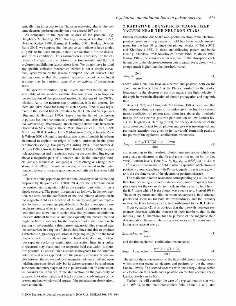
Figure 1. A qualitative sketch of the spectrum I of γ -ray radiation subjectto the one–photon absorption due to pair creation in magnetized vacuumnear a neutron star with B ∼ 1012 G, drawn for the extraordinary (a) andordinary (b) modes and also for the sum of both polarizations (c).

therefore,

h̄ω1 �h̄ω0

(1 + b

2

). (5)

Thus, measuring ω0 and ω1, we can determine the neutron starmagnetic field B = 2Bcr(ω1 − ω0)/ω0.1

Frequencies ω0 and ω1 can be found as the positions of two ab-sorption lines in the pulsar γ -spectrum. From the above-mentionedpolarization dependence of resonances, it is obvious that, if the initialradiation is unpolarized, the depth of these lines at the main anni-hilation and the first cyclotron–annihilation resonances can amountto 50 and 100 per cent, respectively. (Fig. 1).

Unfortunately, this simple picture is complicated by the follow-ing circumstances. First, if the whole surface of a star2 emits in theγ -range, the positions of cyclotron–annihilation resonances in ra-diation spectra emerging from its different pieces are also different(inhomogeneous broadening). The cause is that angle θ 0 between lo-cal magnetic field on the star surface and the direction to the Earth’s

1 It is worth mentioning that, as angle θ disappears in this formula, the methodallows us to determine magnetic field without finding its value which dependson unknown pulsar orientation with respect to the Earth’s observer. This factpresents an essential advantage of the method being discussed.2 Let us mention that the term ‘the surface of a neutron star’ has a somewhatconditional meaning here. As a matter of fact, we use these worlds to denotethe γ -ray source outer surface which, of course, does not necessarily coincidewith the actual surface of a pulsar.

observer as well as the value of the magnetic field changes on starsurface. In any appropriate model of the magnetic field distributionnear a star (for instance, in a dipole model assumed here), this al-teration is essential. Consequently, the positions of absorption linesfrom different pieces of the star surface do not coincide with eachother, and, therefore, these features can not be resolved in the re-sulting spectrum. Thus, the registrable cyclotron–annihilation linesmay be formed in magnetized vacuum only if a γ -ray source is suf-ficiently compact and is located on the star surface or in its nearestneighbourhood where magnetic field is large enough yet.

Secondly, magnetic field in the emitting region must be suffi-ciently high so that the optical depths for the main annihilationand the first cyclotron–annihilation resonances should be compa-rable with unity. On the other hand, it may not be very large be-cause otherwise the optical depth between the two absorption fea-tures becomes essentially larger than unity and the correspondinglines merge. Thus, the value of the magnetic field must lie in a cer-tain interval with the width depending on the source position andstar orientation with respect to the Earth’s observer. As shown inSection 4, this field range is centred at B ∼1012 G. It means that fortypical pulsars a γ -ray source must lie near a star, whereas for mag-netars (Duncan & Thompson 1992; Thompson & Duncan 1995,2001; Thompson, Lyutikov & Kulkarni 2002) with surface fields∼1014–1015 G it must be located at a distance of �10 times the starradius from its centre.

This inference is true for the observations without the separationof polarizations which are only attainable in the γ -range now. Ifthe polarization separation were possible, the upper limit on theallowed field strength would disappear making this method evenmore convenient for the determination of the star magnetic field(please see Conclusion for details).

To determine the above-mentioned magnetic field range we haveto find the optical depth, τ‖,⊥(ω) for the extraordinary (‖) and theordinary (⊥) waves as a function of the photon frequency ω. Thevalues τ‖,⊥(ω) are determined by the coefficients of photon absorp-tion

σ‖,⊥ = σ0‖,⊥ + σ1‖,⊥, (6)

where σ 0 and σ 1 are the contributions from the main annihilationand the first cyclotron–annihilation resonances, respectively. Thevalues ofσ are found as the doubled imaginary parts of the respectivephoton wave numbers obtained from the solution of the dispersionequation following in usual way from the Maxwell equations withthe tensor of the magnetized vacuum permittivity (Belyanin et al.1991, 1997, 2001). To specify the corresponding expressions, let usintroduce the values (Belyanin et al. 1991, 1997, 2001)

Q0‖ = αb sin2 θ exp[−2ω2

/(bω2

0

)](2√

2λc

) ,

Q0⊥ = 0, Q1‖ � 4Q0‖b

, Q1⊥ � 8Q0‖, (7)

where α is the fine structure constant, λc = h̄/(mc) the Comptonwavelength. Under the assumed condition b � 1 for the angles θ

not very close to π/2 (please see the discussion in the next para-graph), the deviation of the wave number from its vacuum value,|δk(ω)| ≡ |k(ω) − ω/c|, is much less than ω/c and we may expandthe dispersion relation over the small parameter δkc/ω.

Inside the resonance regions where |ω/ω0,1 − 1| � 1 and thefrequency detuning is less than the homogeneous resonance width,∣∣∣∣ ω

ω0,1− 1

∣∣∣∣ � 3

[Q0,1‖,⊥ cos2 θλc

(43/2 sin2 θ )

]2/3

, (8)



the collective influence of the virtual electron–positron pairs onthe photon propagation and absorption plays a significant role(Melrose 1974; Shabad 1975; Melrose & Stoneham 1976, 1977;Peres & Shabad 1982) in determining the frequency dependence ofthe absorption coefficients. In result, we obtain that

σ0,1‖,⊥(ω) =√

3ω0,1

c

(λc sin θ Q0,1‖,⊥

4 cos θ

)2/3

×[

1 −(

ω

ω0,1− 1

)2(4 sin2 θ

33/2 Q0,1‖,⊥ cos2 θλc

)4/3]. (9)

From this equation, it follows that the maximal values of Im δk(ω)are achieved at the resonance points where the condition∣∣∣ Imδk(ω0,1)c

ω0,1

∣∣∣ =√

3

2

[λc sin θ Q0,1‖,⊥

4 cos θ

]2/3

� 1 (10)

is satisfied if |θ − π/2| � 4.3 × 10−12 (for b = 0.1), that is, practi-cally for any angle θ . Further, we will not consider the small angleinterval where |Im δk(ω0,1)c/ω0,1| � 1 and assume the inequality|Im δk(ω)c/ω| � 1 to be always true.

In the non-resonance regions whereω/ω0,1 −1�1, butω/ω0,1 −1 � 3[Q0,1‖,⊥ cos2 θλc/(43/2 sin2 θ )]2/3, we arrive at the well-knownformulae for the coefficients of photon absorption which can alsobe obtained using the standard perturbation approach based on thebalance quantum-electrodynamic equations (Belyanin et al. 1991,1997, 2001):

σ0‖,⊥ = Q0‖,⊥sin θ

√ω/ω0 − 1

and σ1‖,⊥ = Q1‖,⊥sin θ

√ω/ω1 − 1

. (11)

Further, we will admit that photon trajectory is a straight line ne-glecting refraction effects in magnetized vacuum which are small inthe assumed case b � 1. To make the calculations, we (as pointed outabove) employ the simplest model of the magnetic field distributionnear a star, that is, consider it to be of the dipole structure:

B(r ) = 3(mr )r

r 5− m

r 3. (12)

Here r is a radius-vector from the centre of a star, m its magnetic mo-ment. From equation (12), it is obvious that due to the field inhomo-geneity values θ and b undergo appreciable variations along the pho-ton trajectories. As shown in the next two sections, the correspond-ing relative alterations of the local resonance frequencies ω0 and ω1

over the trajectory interval with notable absorption are greater thanb0, where b0 is dimensionless magnetic field on the star surface.As a result, the homogeneous resonance width from equation (8) ismuch less than the inhomogenious one (Belyanin et al. 2001) andthe contribution to the optical depth from the non-resonance inter-val (equation 11) is by b0 [sin2 θ/(cos2 θλc Q0,1‖,⊥)]2/3 � 1 timesgreater than that from the resonance one (equation 8). Determiningτ (ω), we can therefore neglect the resonance effects and considerthe non-resonance regions only where the coefficients of photonabsorption are given by equation (11).

Thus, we have the following expressions for the optical depthsfor the extraordinary and ordinary waves:

τ‖,⊥ =∫ ∞

r0

σ‖,⊥dr . (13)

Here r0 is the neutron star radius which is approximately taken tobe equal to 10 km. Let us present τ‖,⊥ as

τ‖,⊥ = τ0‖,⊥ + τ1‖,⊥, (14)

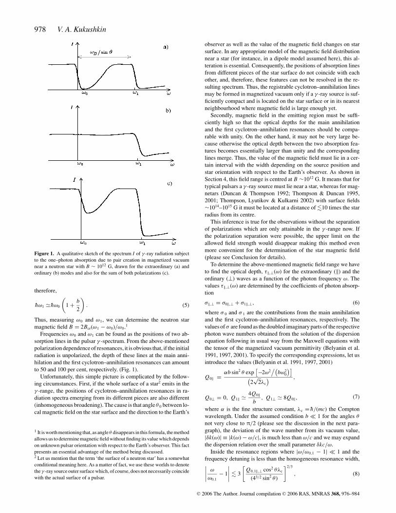
Figure 2. Cross-section layout of two possible sources of γ -radiation: apoint-like source near the star magnetic pole and a disc in the pulsar equa-torial magnetic plane.

where

τ0‖,⊥ =∫ ∞

r0

σ0‖,⊥dr and τ1‖,⊥ =∫ ∞

r0

σ1‖,⊥dr (15)

are the contributions from the main annihilation and the firstcyclotron–annihilation resonances, respectively. As Q0⊥ = 0, thenτ 0⊥ = 0 and τ⊥ = τ 1⊥.

To obtain from equation (13) the allowed magnetic field interval,we need to specify a γ -ray source form and position. In the nexttwo sections, we consider situations when one is located near a starmagnetic pole or is represented by a narrow in the meridional di-rection and radially thin disc lying near the pulsar magnetic equator(Fig. 2).

3 A P O L E S O U R C E I N T H E D I P O L E

M AG N E T I C F I E L D

Let us consider an idealized point γ -ray source at the northern (fordefiniteness’ sake) magnetic pole of a neutron star (Fig. 2). Due to theaxial symmetry, we can specify the direction of photon propagationby its angle with the neutron star magnetic moment m only. In thepresent geometry, this angle coincides with θ 0 ≡ θ (r = r 0). Fromequation (12) it is easy to see that for small values of (r − r 0)/r 0 ≡ρ with accuracy up to ρ2, inclusively, the following approximationsare valid:

sin θ (r ) � sin θ0

[1 − 3ρ cos θ0

2− ρ2

(9 + 7 cos2 θ0

)8

], (16)

b(r ) � b0p

[1 − 3ρ cos θ0 − 5ρ2

(4 − sin2 θ0

)8

], (17)

where b0p = 2m/(B cr 30) is the dimensionless magnetic field strength

on the pole. Using these expressions, we find that the coordinatedependence of the exponent power in equation (7) for Q values atsmall ρ is given by the formula

2ω2ρ2(

33 − 18 sin2 θ0

)[16b0pω

20(r0)

] , (18)

where ω0(r 0) = 2mc2/(h̄ sin θ 0) is the frequency of the main anni-hilation resonance at the pole.

Equation (16) shows that sin θ (r) decreases with the increase of rso that the frequencies ω0(r ), ω1(r ) grow along the photon trajecto-ries. From equation (18) we can also conclude that the coefficientsQ decrease exponentially with the growth of r − r 0, so that the


980 V. A. Kukushkin

integrals over r in the expressions for the optical depth (13), (14),(15) may be evaluated as the products of the integrands at the initialpoint and r 0,1effp ≡ min (r ∗p − r 0, r 0,1∗ − r 0) for τ 0,1, respectively,

τ0‖,⊥ = σ0‖,⊥r0effp and τ1‖,⊥ = σ1‖,⊥r1effp. (19)

Here, r ∗p(ω) is the point where the expression (18) is equal to unityand, consequently, the coefficients Q decrease by e times, and r 0,1∗equals the distances between the star centre and the point where thelocal threshold frequencies, ω0(r) and ω1(r ), respectively, becomelarger than the photon frequency ω. [If ω is sufficiently small sothat ω < ω0,1(r ) even for r = r 0, the values of r 0,1∗ are defined asequal to r0.] Equation (18) shows that for the frequencies ω closeto ω0(r 0) and ω1(r 0) (which are only being studied in this paper)we have [r∗p(ω) − r0]/r0 ∼ √

b0p � 1 for the case b0p � 1 beingconsidered. It allows us to use the approximate expressions (16) and(17) for sin θ (r) and b(r), respectively.

As ω0(r ) and ω1(r ) increase with the growth of r, it is obviousthat τ 0 and τ 1 as functions of ω have the maximum values for

ω0mp = ω0[r∗p(ω0mp)] (20)

and

ω1mp = ω1[r∗p(ω1mp)], (21)

respectively. For smaller ω we have r 0,1∗ < r ∗p, so that only a partof the interval r ∗p − r 0 will give the contributions to the τ 0,1. Onthe other hand, for larger ω the denominators in equation (11) willincrease so that σ 0,1 and, consequently, τ 0,1 will decrease.

As the value of r ∗p itself is a function of ω0,1mp, equations (20),(21) allow us to find ω0,1mp and the corresponding values of r ∗p.With accuracy up to

√b0p, inclusively, we obtain

r∗p(ω0mp) = r∗p(ω1mp) = r0

(1 + 2

√2b0p√

33 − 18 sin2 θ0

), (22)

ω0mp = ω0

(1 + 3 cos θ0

√2b0p√

33 − 18 sin2 θ0

), (23)

ω1mp = ω0mp. (24)

Let us first consider the optical depth τ ‖ for the extraordi-nary wave. According to the formulae obtained, for a pole source(r∗p − r0)/r0 ∼ √

b0p (see equation 22), that is, the distancer∗p − r 0 is rather large. This leads to the distinct variations of θ

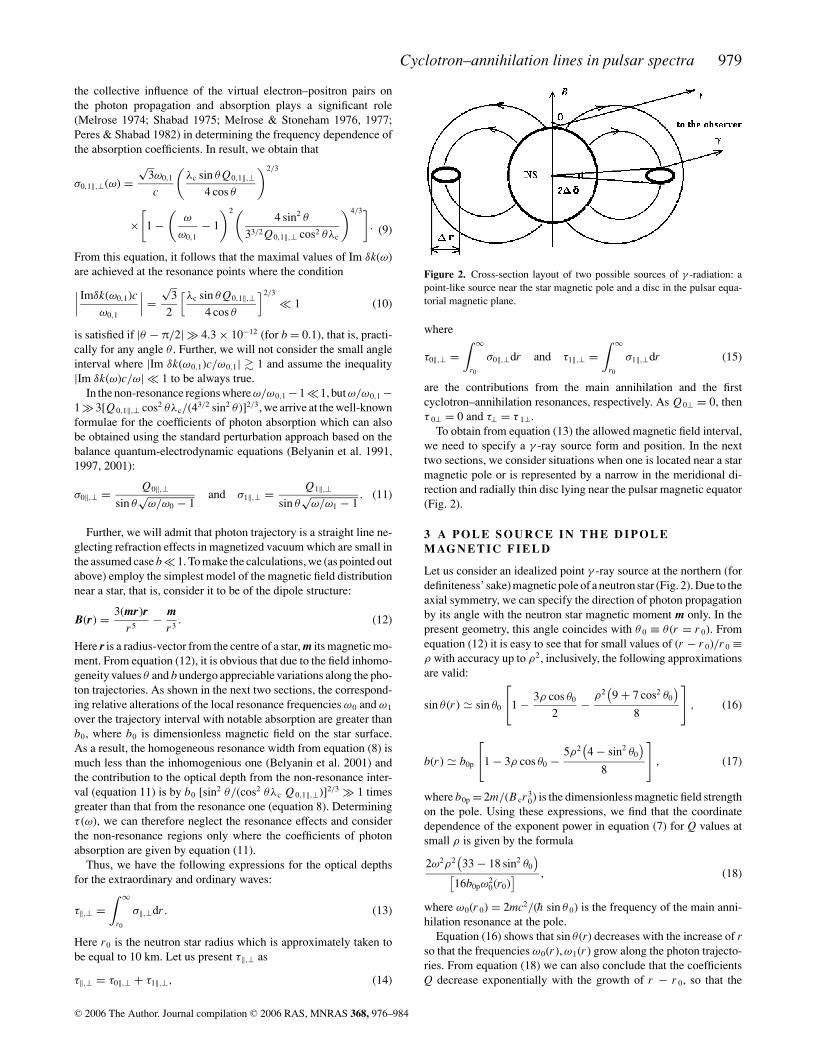
and b along the photon trajectory and, as a result, to the remark-able deviation of the resonance frequencies ω0mp = ω0(r ∗p) andω1mp = ω1(r ∗p) from their values ω0(r 0) and ω1(r 0) at the pole andstrong inhomogeneous broadening of the resonances. This causesthe main cyclotron–annihilation resonance covering, practically, allthe inter-resonance interval so that the intensity rise between thecorresponding absorption lines becomes rather small and difficultto measure.

As far as the optical depth for the ordinary wave is concerned, ac-cording to equations (7), (11) it is determined by the first cyclotron–annihilation resonance only. So, τ⊥ = τ 1⊥ and in the frequencyinterval being considered only one absorption line centred at thefrequency ω1mp will appear in the spectrum of this wave.

Thus, all of these may make the cyclotron–annihilation absorptionlines in the resulting spectrum of the pulsar γ -radiation (which isobtained by summing up the spectral intensities of the extraordinaryand ordinary waves) hard to resolve and can therefore significantly

Figure 3. The spectrum I of the γ -radiation from a pole source undergoingone–photon absorption in magnetized vacuum in comparison with its non-perturbed value, I0, for different magnetic fields B = 3.1 × 1012 G (dot–dashed line), B = 3.3 × 1012 G (dashed line), and B = 3.5 × 1012 G (solidline). θ 0 = 80◦.

hamper field measuring. This qualitative conclusion is confirmed bynumerical simulations which show that the neutron star γ -spectra donot exhibit distinct cyclotron–annihilation lines not only for smallθ 0 � 1 (in accordance with the previous studies of this problem,e.g. Harding et al. 1997; Baring & Harding 2001; Rudak et al. 2002),but also for large θ 0 � 60◦ (Fig. 3).

It is also worth mentioning that in this section we deal with anidealized point source. But it is clear that taking into account finitesource dimensions would lead to the additional variations of sin θ 0

and b0p in the emitting region and, as a consequence, to the additionalinhomogeneous broadening of the lines. So, all the inferences of thissection also hold true for a real pole source.

4 A N E QUATO R I A L S O U R C E I N A D I P O L E

M AG N E T I C F I E L D

Now let us consider the case when a γ -ray source is located nearthe star magnetic equator (Fig. 2). First, we will discuss an idealizedinfinitely narrow in the meridional direction and radially thin disclying on the star surface. Specifying position on the observed sideof the source by the azimuthal angle φ, − π/2 < φ < π/2, it is easyto find that, with accuracy up to ρ2, inclusively,

b = b0e

[1 − 3ρ sin θ0 cos φ − ρ2 sin2 θ0(3 + 5 cos2 φ)

2

], (25)

sin θ (r )=sin θ0

[1+ 6ρ cos2 θ0 cos φ

sin θ0+3ρ2

(2+cos2 θ0

)cot2 θ0

]1/2

,

(26)

where b0e = m/B cr 30 is the dimensionless field on the equator.

Using these expressions, we find that the coordinate dependenceof the exponent power in equation (7) for small ρ is given by

ω2

b0eω20(r0)

{6ρ

(1 + cos2 θ0

)cos φ

sin θ0+ ρ2

[(3 + 5 cos2 φ) sin2 θ0

+ 3 cot2 θ0

(2 + cos2 θ0

)]}(27)

and determine the value r∗e(ω) on the analogy of the pole source caseas a distance where expression (27) equals unity. It can be shown



that (with accuracy up to b0e inclusively) r∗e(ω0me) = r∗e(ω1me) ≡r∗e, where r∗e = r∗e(ω0(r 0). For cos φ � √

b0e, we have (r∗e −r 0)/r 0 ∝ b0e whereas in the opposite case cos φ �

√b0e we obtain

(r∗e − r0)/r0 ∝ √b0e.

The important difference of equation (26) from that for the polesource (equation 16) is that sin θ increases with growing r. There-fore, the local resonance frequencies ω0(r ) and ω1(r ) decrease alongthe photon trajectory. So we conclude that τ 0,1 as functions of ω havemaximum values for

ω0me = ω0(r0) (28)

and

ω1me = ω1(r0), (29)

respectively. For smaller ω we have r ∗0,1 > r 0, so that only a part(with the length r∗e − r ∗0,1 if r ∗0,1 < r∗e or 0 if r ∗0,1 > r∗e) of theinterval r∗e − r 0 will give contributions to the τ 0,1. On the otherhand, for larger ω the denominators in equation (11) will increaseso that σ 0,1 and, consequently, τ 0,1 will decrease.

Now, as in equation (19), we can approximate the expressions forthe optical depth 13, 14 and 15 as the products of the integrands atthe point r∗e and values r 0,1effe. The latter, in contrast to the definitionof r 0,1effp in the previous section for the pole source, equals zero forr ∗0,1 >r∗e, r∗e − r ∗0,1 for r 0 < r ∗0,1 < r∗e, and r∗e for r ∗0,1 < r 0.

To analyse the spectra of the extraordinary and ordinary waves,we define the effective optical depth by averaging it over the source:

τ‖,⊥effe = − ln

{∫ π/2

−π/2

exp[−τ‖,⊥(φ)](

1 − sin2 θ0 sin2 φ)1/2

dφ

/∫ π/2

−π/2

√1 − sin2 θ0 sin2 φdφ

}, (30)

where√

1 − sin2 θ0 sin2 φ is the cosine of the angle between a planelocally normal to the equator and the direction to the Earth’s ob-server. In this formula we used a natural assumption that the prop-erties of the disc γ -emission do not depend on angle φ and possesslongitudinal symmetry. This inference follows from the fact that inthe present geometry all parts of the disc are placed in the samemagnetic field orthogonal to its plane.

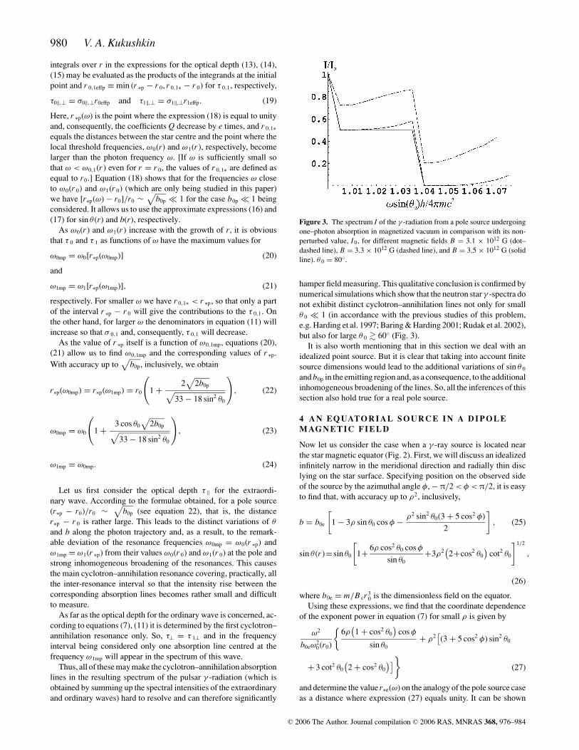
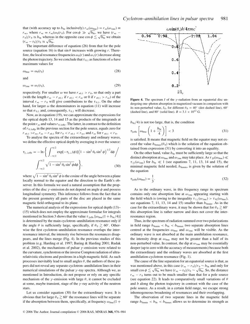
The numerical analysis of the expressions for optical depth (13)–(15) which does not employ the approximate formulae for integralsmentioned in Section 3 shows that the value τ ‖effe [ω0me(1 + b0e/4)]is determined by the main cyclotron–annihilation resonance only ifthe angle θ is sufficiently large, specifically, if θ 0 � 60◦. Other-wise the first cyclotron–annihilation resonance overlaps the inter-resonance interval, the intensity rise between the resonances disap-pears, and the lines merge (Fig. 4). In the previous studies of thisproblem (e.g. Harding et al. 1997; Baring & Harding 2001; Rudaket al. 2002), the mechanisms of pulsar γ -emission were related tothe curvature, synchrotron or the inverse Compton radiation of ultra-relativistic electrons and positrons in a high magnetic field. As suchprocesses inevitably lead to small angles θ , the authors of these pa-pers did not reveal any separate cyclotron–annihilation lines in theirnumerical simulations of the pulsar γ -ray spectra. Although we, asmentioned in Introduction, do not propose or rely on any specificmechanism of the γ -emission with large θ , it cannot be excludedat some, maybe transient, stage of the γ -ray activity of the neutronstars.

Let us consider equation (30) for the extraordinary wave. It isobvious that for large θ 0 � 60◦ the resonance lines will be separateif the absorption between them, specifically, at frequency ω0me(1 +

Figure 4. The spectrum I of the γ -radiation from an equatorial disc un-dergoing one–photon absorption in magnetized vacuum in comparison withits non-perturbed value, I0, for different θ 0 = 40◦ (dot–dashed line), 60◦(dashed line), and 80◦ (solid line). B = 3.1 × 1012 G.

b0e/4) is not too large, that is, the condition

τ‖effe

[ω0me

(1 + b0e

4

)]< 3 (31)

is satisfied. It means that magnetic field on the equator may not ex-ceed the value b0emax(θ 0) which is the solution of the equation ob-tained from expression (31) by converting it into an equality.

On the other hand, value b0e must be sufficiently large so that thedistinct absorption at ω0me and ω1me may take place. As τ ‖0(ω0me) �τ ‖1(ω1me) for b0e � 1 (see equations 7, 11, 13, 14 and 15), theminimal magnetic field needed, b0emin, is given by the solution ofthe equation

τ‖effe(ω0me) = 1

3. (32)

As to the ordinary wave, in this frequency range its spectrumcontains only one absorption line at ω1me appearing starting withthe field which is (owing to the inequality τ 1⊥(ω1me) > τ 0‖(ω0me),see equations 7, 11, 13, 14 and 15) smaller than b0emin. As in thecase for the extraordinary wave, it may be shown that for θ 0 � 60◦

this absorption line is rather narrow and does not cover the inter-resonance region.

Thus, in the spectrum of radiation summed over two polarizationsin field range b0emin < b0e < b0emax two separate absorption linescentred at the frequencies ω0me and ω1me will be visible. As theordinary wave is not absorbed at the main annihilation resonance,the intensity drop at ω0me may not be greater than a half of itsnon-perturbed value. In contrast, the dip at ω1me may be essentiallydeeper (up to zero with the accuracy of measurements) because boththe extraordinary and the ordinary waves are absorbed at the firstannihilation-cyclotron resonance (Fig. 1).

The cause of the line separation for an equatorial source is that, aswas mentioned above, in this case (r∗e − r 0)/r 0 ∼ b0e and only forsmall cos φ �

√b0e we have (r∗e − r0)/r0 ∼ √

b0e. So, the distancer∗e − r 0 turns out to be much smaller than that for a pole source(see equation 22). It leads to comparatively small variations of θ

and b along the photon trajectory in contrast with the case of thepole source. As a result, in a certain field range, we escape stronginhomogeneous broadening of resonances and their overlapping.

The observation of two separate lines in the magnetic fieldrange b0emin < b0e < b0emax allows us to determine its strength as


982 V. A. Kukushkin

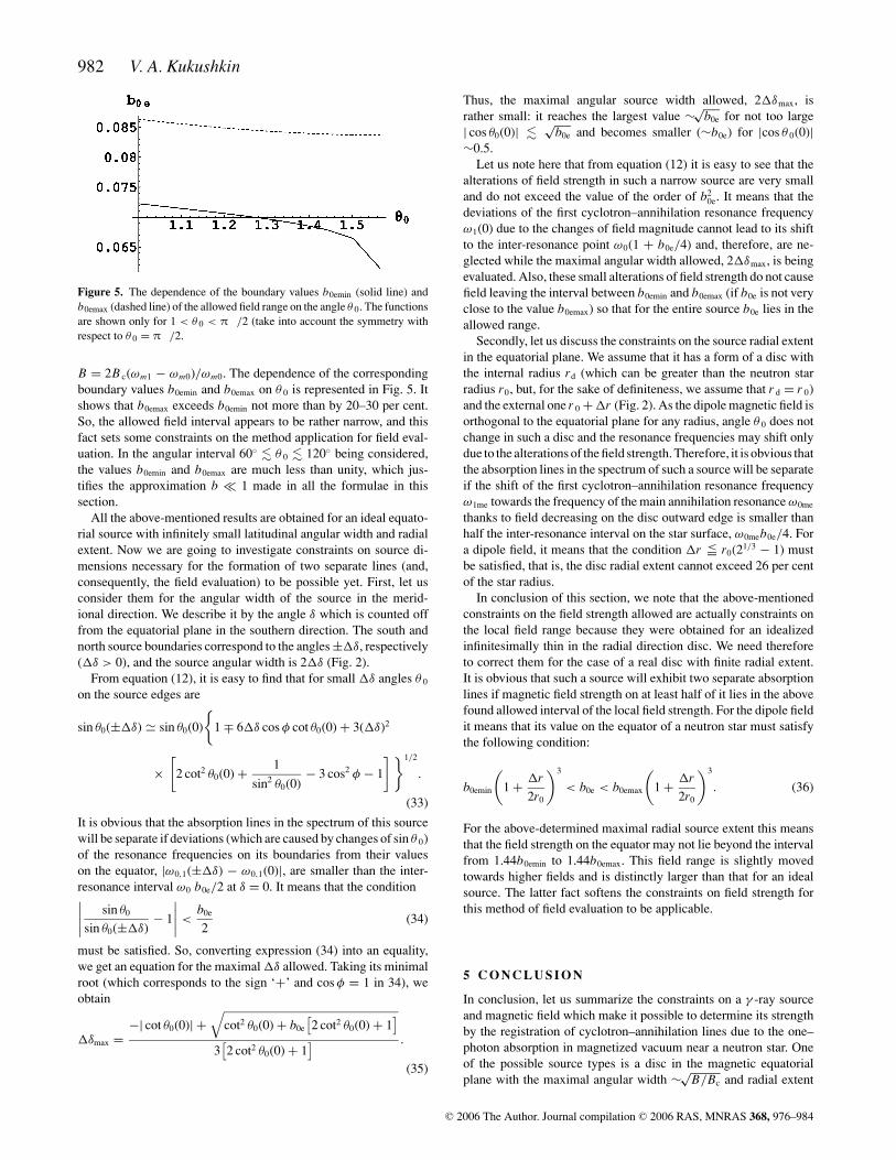
Figure 5. The dependence of the boundary values b0emin (solid line) andb0emax (dashed line) of the allowed field range on the angle θ 0. The functionsare shown only for 1 < θ 0 < π /2 (take into account the symmetry withrespect to θ 0 = π /2.

B = 2B c(ωm1 − ωm0)/ωm0. The dependence of the correspondingboundary values b0emin and b0emax on θ 0 is represented in Fig. 5. Itshows that b0emax exceeds b0emin not more than by 20–30 per cent.So, the allowed field interval appears to be rather narrow, and thisfact sets some constraints on the method application for field eval-uation. In the angular interval 60◦ � θ 0 � 120◦ being considered,the values b0emin and b0emax are much less than unity, which jus-tifies the approximation b � 1 made in all the formulae in thissection.

All the above-mentioned results are obtained for an ideal equato-rial source with infinitely small latitudinal angular width and radialextent. Now we are going to investigate constraints on source di-mensions necessary for the formation of two separate lines (and,consequently, the field evaluation) to be possible yet. First, let usconsider them for the angular width of the source in the merid-ional direction. We describe it by the angle δ which is counted offfrom the equatorial plane in the southern direction. The south andnorth source boundaries correspond to the angles ± δ, respectively( δ > 0), and the source angular width is 2 δ (Fig. 2).

From equation (12), it is easy to find that for small δ angles θ 0

on the source edges are

sin θ0(± δ) � sin θ0(0)

{1 ∓ 6 δ cos φ cot θ0(0) + 3( δ)2

×[

2 cot2 θ0(0) + 1

sin2 θ0(0)− 3 cos2 φ − 1

]}1/2

.

(33)

It is obvious that the absorption lines in the spectrum of this sourcewill be separate if deviations (which are caused by changes of sin θ 0)of the resonance frequencies on its boundaries from their valueson the equator, |ω0,1(± δ) − ω0,1(0)|, are smaller than the inter-resonance interval ω0 b0e/2 at δ = 0. It means that the condition∣∣∣∣ sin θ0

sin θ0(± δ)− 1

∣∣∣∣ <b0e

2(34)

must be satisfied. So, converting expression (34) into an equality,we get an equation for the maximal δ allowed. Taking its minimalroot (which corresponds to the sign ‘+’ and cos φ = 1 in 34), weobtain

δmax =−| cot θ0(0)| +

√cot2 θ0(0) + b0e

[2 cot2 θ0(0) + 1

]3[2 cot2 θ0(0) + 1

] .

(35)

Thus, the maximal angular source width allowed, 2 δmax, israther small: it reaches the largest value ∼√

b0e for not too large| cos θ0(0)| �

√b0e and becomes smaller (∼b0e) for |cos θ 0(0)|

∼0.5.Let us note here that from equation (12) it is easy to see that the

alterations of field strength in such a narrow source are very smalland do not exceed the value of the order of b2

0e. It means that thedeviations of the first cyclotron–annihilation resonance frequencyω1(0) due to the changes of field magnitude cannot lead to its shiftto the inter-resonance point ω0(1 + b0e/4) and, therefore, are ne-glected while the maximal angular width allowed, 2 δmax, is beingevaluated. Also, these small alterations of field strength do not causefield leaving the interval between b0emin and b0emax (if b0e is not veryclose to the value b0emax) so that for the entire source b0e lies in theallowed range.

Secondly, let us discuss the constraints on the source radial extentin the equatorial plane. We assume that it has a form of a disc withthe internal radius rd (which can be greater than the neutron starradius r0, but, for the sake of definiteness, we assume that r d = r 0)and the external one r 0 + r (Fig. 2). As the dipole magnetic field isorthogonal to the equatorial plane for any radius, angle θ 0 does notchange in such a disc and the resonance frequencies may shift onlydue to the alterations of the field strength. Therefore, it is obvious thatthe absorption lines in the spectrum of such a source will be separateif the shift of the first cyclotron–annihilation resonance frequencyω1me towards the frequency of the main annihilation resonance ω0me

thanks to field decreasing on the disc outward edge is smaller thanhalf the inter-resonance interval on the star surface, ω0meb0e/4. Fora dipole field, it means that the condition r <= r0(21/3 − 1) mustbe satisfied, that is, the disc radial extent cannot exceed 26 per centof the star radius.

In conclusion of this section, we note that the above-mentionedconstraints on the field strength allowed are actually constraints onthe local field range because they were obtained for an idealizedinfinitesimally thin in the radial direction disc. We need thereforeto correct them for the case of a real disc with finite radial extent.It is obvious that such a source will exhibit two separate absorptionlines if magnetic field strength on at least half of it lies in the abovefound allowed interval of the local field strength. For the dipole fieldit means that its value on the equator of a neutron star must satisfythe following condition:

b0emin

(1 + r

2r0

)3

< b0e < b0emax

(1 + r

2r0

)3

. (36)

For the above-determined maximal radial source extent this meansthat the field strength on the equator may not lie beyond the intervalfrom 1.44b0emin to 1.44b0emax. This field range is slightly movedtowards higher fields and is distinctly larger than that for an idealsource. The latter fact softens the constraints on field strength forthis method of field evaluation to be applicable.

5 C O N C L U S I O N

In conclusion, let us summarize the constraints on a γ -ray sourceand magnetic field which make it possible to determine its strengthby the registration of cyclotron–annihilation lines due to the one–photon absorption in magnetized vacuum near a neutron star. Oneof the possible source types is a disc in the magnetic equatorialplane with the maximal angular width ∼√

B/Bc and radial extent



Figure 6. The dependence of the boundary values b0emin(1 + r/2r 0)3

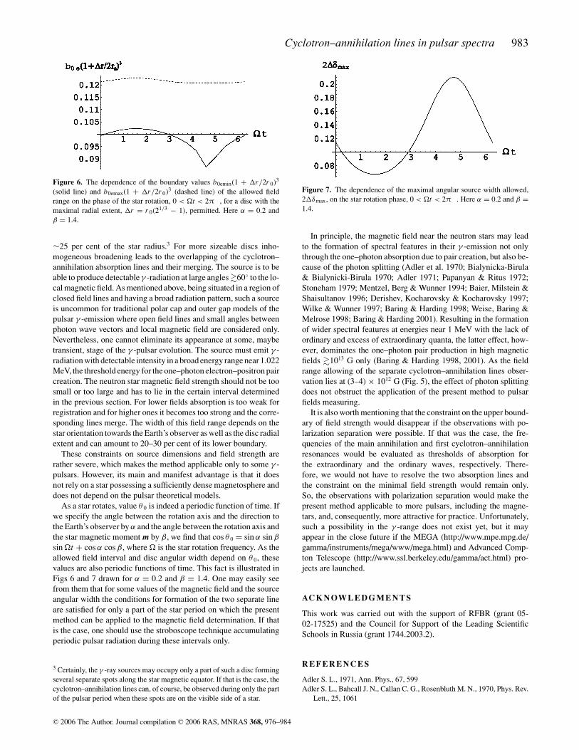
(solid line) and b0emax(1 + r/2r 0)3 (dashed line) of the allowed fieldrange on the phase of the star rotation, 0 < �t < 2π , for a disc with themaximal radial extent, r = r 0(21/3 − 1), permitted. Here α = 0.2 andβ = 1.4.

∼25 per cent of the star radius.3 For more sizeable discs inho-mogeneous broadening leads to the overlapping of the cyclotron–annihilation absorption lines and their merging. The source is to beable to produce detectable γ -radiation at large angles �60◦ to the lo-cal magnetic field. As mentioned above, being situated in a region ofclosed field lines and having a broad radiation pattern, such a sourceis uncommon for traditional polar cap and outer gap models of thepulsar γ -emission where open field lines and small angles betweenphoton wave vectors and local magnetic field are considered only.Nevertheless, one cannot eliminate its appearance at some, maybetransient, stage of the γ -pulsar evolution. The source must emit γ -radiation with detectable intensity in a broad energy range near 1.022MeV, the threshold energy for the one–photon electron–positron paircreation. The neutron star magnetic field strength should not be toosmall or too large and has to lie in the certain interval determinedin the previous section. For lower fields absorption is too weak forregistration and for higher ones it becomes too strong and the corre-sponding lines merge. The width of this field range depends on thestar orientation towards the Earth’s observer as well as the disc radialextent and can amount to 20–30 per cent of its lower boundary.

These constraints on source dimensions and field strength arerather severe, which makes the method applicable only to some γ -pulsars. However, its main and manifest advantage is that it doesnot rely on a star possessing a sufficiently dense magnetosphere anddoes not depend on the pulsar theoretical models.

As a star rotates, value θ 0 is indeed a periodic function of time. Ifwe specify the angle between the rotation axis and the direction tothe Earth’s observer by α and the angle between the rotation axis andthe star magnetic moment m by β, we find that cos θ 0 = sin α sin β

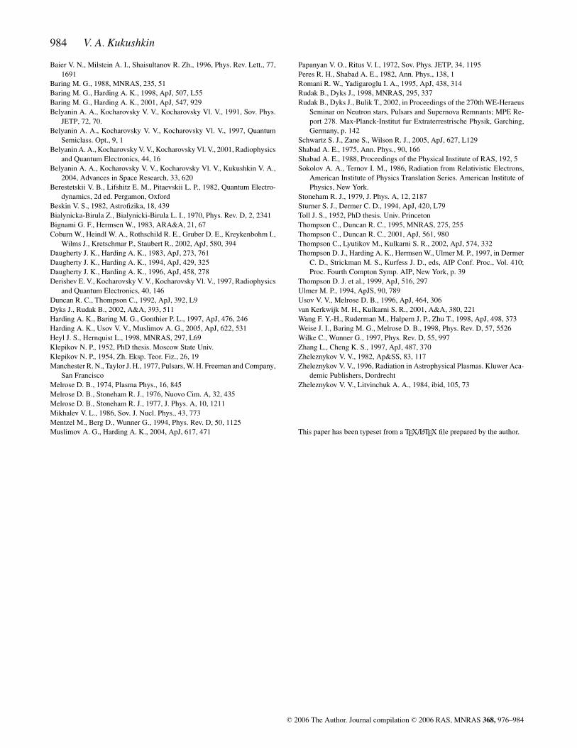
sin �t + cos α cos β, where � is the star rotation frequency. As theallowed field interval and disc angular width depend on θ 0, thesevalues are also periodic functions of time. This fact is illustrated inFigs 6 and 7 drawn for α = 0.2 and β = 1.4. One may easily seefrom them that for some values of the magnetic field and the sourceangular width the conditions for formation of the two separate lineare satisfied for only a part of the star period on which the presentmethod can be applied to the magnetic field determination. If thatis the case, one should use the stroboscope technique accumulatingperiodic pulsar radiation during these intervals only.

3 Certainly, the γ -ray sources may occupy only a part of such a disc formingseveral separate spots along the star magnetic equator. If that is the case, thecyclotron–annihilation lines can, of course, be observed during only the partof the pulsar period when these spots are on the visible side of a star.

Figure 7. The dependence of the maximal angular source width allowed,2 δmax, on the star rotation phase, 0 < �t < 2π . Here α = 0.2 and β =1.4.

In principle, the magnetic field near the neutron stars may leadto the formation of spectral features in their γ -emission not onlythrough the one–photon absorption due to pair creation, but also be-cause of the photon splitting (Adler et al. 1970; Bialynicka-Birula& Bialynicki-Birula 1970; Adler 1971; Papanyan & Ritus 1972;Stoneham 1979; Mentzel, Berg & Wunner 1994; Baier, Milstein &Shaisultanov 1996; Derishev, Kocharovsky & Kocharovsky 1997;Wilke & Wunner 1997; Baring & Harding 1998; Weise, Baring &Melrose 1998; Baring & Harding 2001). Resulting in the formationof wider spectral features at energies near 1 MeV with the lack ofordinary and excess of extraordinary quanta, the latter effect, how-ever, dominates the one–photon pair production in high magneticfields �1013 G only (Baring & Harding 1998, 2001). As the fieldrange allowing of the separate cyclotron–annihilation lines obser-vation lies at (3–4) × 1012 G (Fig. 5), the effect of photon splittingdoes not obstruct the application of the present method to pulsarfields measuring.

It is also worth mentioning that the constraint on the upper bound-ary of field strength would disappear if the observations with po-larization separation were possible. If that was the case, the fre-quencies of the main annihilation and first cyclotron–annihilationresonances would be evaluated as thresholds of absorption forthe extraordinary and the ordinary waves, respectively. There-fore, we would not have to resolve the two absorption lines andthe constraint on the minimal field strength would remain only.So, the observations with polarization separation would make thepresent method applicable to more pulsars, including the magne-tars, and, consequently, more attractive for practice. Unfortunately,such a possibility in the γ -range does not exist yet, but it mayappear in the close future if the MEGA (http://www.mpe.mpg.de/gamma/instruments/mega/www/mega.html) and Advanced Comp-ton Telescope (http://www.ssl.berkeley.edu/gamma/act.html) pro-jects are launched.

AC K N OW L E D G M E N T S

This work was carried out with the support of RFBR (grant 05-02-17525) and the Council for Support of the Leading ScientificSchools in Russia (grant 1744.2003.2).

R E F E R E N C E S

Adler S. L., 1971, Ann. Phys., 67, 599Adler S. L., Bahcall J. N., Callan C. G., Rosenbluth M. N., 1970, Phys. Rev.

Lett., 25, 1061


984 V. A. Kukushkin

Baier V. N., Milstein A. I., Shaisultanov R. Zh., 1996, Phys. Rev. Lett., 77,1691

Baring M. G., 1988, MNRAS, 235, 51Baring M. G., Harding A. K., 1998, ApJ, 507, L55Baring M. G., Harding A. K., 2001, ApJ, 547, 929Belyanin A. A., Kocharovsky V. V., Kocharovsky Vl. V., 1991, Sov. Phys.

JETP, 72, 70.Belyanin A. A., Kocharovsky V. V., Kocharovsky Vl. V., 1997, Quantum

Semiclass. Opt., 9, 1Belyanin A. A., Kocharovsky V. V., Kocharovsky Vl. V., 2001, Radiophysics

and Quantum Electronics, 44, 16Belyanin A. A., Kocharovsky V. V., Kocharovsky Vl. V., Kukushkin V. A.,

2004, Advances in Space Research, 33, 620Berestetskii V. B., Lifshitz E. M., Pitaevskii L. P., 1982, Quantum Electro-

dynamics, 2d ed. Pergamon, OxfordBeskin V. S., 1982, Astrofizika, 18, 439Bialynicka-Birula Z., Bialynicki-Birula L. I., 1970, Phys. Rev. D, 2, 2341Bignami G. F., Hermsen W., 1983, ARA&A, 21, 67Coburn W., Heindl W. A., Rothschild R. E., Gruber D. E., Kreykenbohm I.,

Wilms J., Kretschmar P., Staubert R., 2002, ApJ, 580, 394Daugherty J. K., Harding A. K., 1983, ApJ, 273, 761Daugherty J. K., Harding A. K., 1994, ApJ, 429, 325Daugherty J. K., Harding A. K., 1996, ApJ, 458, 278Derishev E. V., Kocharovsky V. V., Kocharovsky Vl. V., 1997, Radiophysics

and Quantum Electronics, 40, 146Duncan R. C., Thompson C., 1992, ApJ, 392, L9Dyks J., Rudak B., 2002, A&A, 393, 511Harding A. K., Baring M. G., Gonthier P. L., 1997, ApJ, 476, 246Harding A. K., Usov V. V., Muslimov A. G., 2005, ApJ, 622, 531Heyl J. S., Hernquist L., 1998, MNRAS, 297, L69Klepikov N. P., 1952, PhD thesis. Moscow State Univ.Klepikov N. P., 1954, Zh. Eksp. Teor. Fiz., 26, 19Manchester R. N., Taylor J. H., 1977, Pulsars, W. H. Freeman and Company,

San FranciscoMelrose D. B., 1974, Plasma Phys., 16, 845Melrose D. B., Stoneham R. J., 1976, Nuovo Cim. A, 32, 435Melrose D. B., Stoneham R. J., 1977, J. Phys. A, 10, 1211Mikhalev V. L., 1986, Sov. J. Nucl. Phys., 43, 773Mentzel M., Berg D., Wunner G., 1994, Phys. Rev. D, 50, 1125Muslimov A. G., Harding A. K., 2004, ApJ, 617, 471

Papanyan V. O., Ritus V. I., 1972, Sov. Phys. JETP, 34, 1195Peres R. H., Shabad A. E., 1982, Ann. Phys., 138, 1Romani R. W., Yadigaroglu I. A., 1995, ApJ, 438, 314Rudak B., Dyks J., 1998, MNRAS, 295, 337Rudak B., Dyks J., Bulik T., 2002, in Proceedings of the 270th WE-Heraeus

Seminar on Neutron stars, Pulsars and Supernova Remnants; MPE Re-port 278. Max-Planck-Institut fur Extraterrestrische Physik, Garching,Germany, p. 142

Schwartz S. J., Zane S., Wilson R. J., 2005, ApJ, 627, L129Shabad A. E., 1975, Ann. Phys., 90, 166Shabad A. E., 1988, Proceedings of the Physical Institute of RAS, 192, 5Sokolov A. A., Ternov I. M., 1986, Radiation from Relativistic Electrons,

American Institute of Physics Translation Series. American Institute ofPhysics, New York.

Stoneham R. J., 1979, J. Phys. A, 12, 2187Sturner S. J., Dermer C. D., 1994, ApJ, 420, L79Toll J. S., 1952, PhD thesis. Univ. PrincetonThompson C., Duncan R. C., 1995, MNRAS, 275, 255Thompson C., Duncan R. C., 2001, ApJ, 561, 980Thompson C., Lyutikov M., Kulkarni S. R., 2002, ApJ, 574, 332Thompson D. J., Harding A. K., Hermsen W., Ulmer M. P., 1997, in Dermer

C. D., Strickman M. S., Kurfess J. D., eds, AIP Conf. Proc., Vol. 410;Proc. Fourth Compton Symp. AIP, New York, p. 39

Thompson D. J. et al., 1999, ApJ, 516, 297Ulmer M. P., 1994, ApJS, 90, 789Usov V. V., Melrose D. B., 1996, ApJ, 464, 306van Kerkwijk M. H., Kulkarni S. R., 2001, A&A, 380, 221Wang F. Y.-H., Ruderman M., Halpern J. P., Zhu T., 1998, ApJ, 498, 373Weise J. I., Baring M. G., Melrose D. B., 1998, Phys. Rev. D, 57, 5526Wilke C., Wunner G., 1997, Phys. Rev. D, 55, 997Zhang L., Cheng K. S., 1997, ApJ, 487, 370Zheleznykov V. V., 1982, Ap&SS, 83, 117Zheleznykov V. V., 1996, Radiation in Astrophysical Plasmas. Kluwer Aca-

demic Publishers, DordrechtZheleznykov V. V., Litvinchuk A. A., 1984, ibid, 105, 73

This paper has been typeset from a TEX/LATEX file prepared by the author.


Documents

Formation of cyclotron–annihilation lines in magnetized vacuum near neutron stars