Transaction B: Mechanical EngineeringVol. 16, No. 1, pp. 101{109c Sharif University of Technology, February 2009

Research Note

Formulation and Numerical Solution of RobotManipulators in Point-to-Point Motionwith Maximum Load Carrying Capacity

M.H. Korayem1;� and A. Nikoobin1

Abstract. In this paper, a formulation is developed for obtaining the optimal trajectory of robotmanipulators to maximize the load carrying capacity for a given point-to-point task. The presented methodis based on open loop optimal control. The indirect approach is employed to derive optimality conditionsbased on Pontryagin's Minimum Principle. The obtained necessary conditions for optimality lead to atwo-point boundary-value problem solved via a multiple shooting method with the BVP4C command inMATLAB r . Since the carrying payload is one of the system parameters, a computational algorithm isdeveloped, which provides the capability of calculating the maximum payload for a point-to-point task. Themain advantage of this method is obtaining various optimal trajectories with di�erent maximum payloadsand path characteristics by changing the penalty matrices values. To demonstrate the e�ciency of theproposed method and algorithm in obtaining the maximum payload trajectory, simulation is performed ona two-link manipulator.

Keywords: Robot manipulator; Maximum payload; Optimal trajectory; Optimal control.

INTRODUCTION

In order to increase the productivity and economicusage of manipulators, �nding the full load motionfor a given point-to-point task has received increasingattention over the two last decades. The Maximum Al-lowable Load (MAL) of a manipulator is often de�nedas the maximum payload that the manipulator canrepeatedly lift in its fully extended con�guration [1].Another de�nition of maximum payload is the maxi-mum value of the load that a robot manipulator is ableto carry on a desired trajectory, which is based on theconsideration of inertia e�ects on this desired path [2].Finding the maximum payload that a manipulatorcan carry between given initial and �nal positions ofthe end-e�ector is yet another way of obtaining theMAL. In this case, the joint trajectory and applied

1. Robotic Research Laboratory, Department of Mechanical En-gineering, Iran University of Science and Technology, P.O.Box 18846, Tehran, Iran.

*. Corresponding author. E-mail: hkorayem@iust.ac.ir

Received 1 April 2007; received in revised form 25 June 2007;accepted 16 July 2007

torque in each motor should be found, so that themaximum load can be carried between two pointsand which is formulated as a trajectory optimizationproblem.

Much of the previous work on determining maxi-mum payload trajectory is based on Iterative LinearProgramming (ILP). The �rst formulation of thismethod for a simple robot manipulator was presentedby Wang and Ravani [3]. Korayem and Gharibluused the ILP method for the MAL calculation of arigid mobile manipulator [4]. For a exible mobilemanipulator, a computational algorithm, to determinethe maximum payload trajectory via linearizing thedynamic equation and constraints, is also presented onthe basis of the ILP approach [5,6]. The linearizingprocedure in the ILP method and its convergence isa challenging issue, especially when nonlinear termsare large and uctuating, e.g. in problems with aconsideration of exibility in the joints or links, gravityacceleration or high speed motion. Wang et al. haveused another approach to determine the maximumpayload, based on a solution of the optimal controlproblem with a direct method [7]. The basic idea of

102 M.H. Korayem and A. Nikoobin

this work is to parameterize the joint trajectories by theuse of B-Spline functions and by tuning the parametersin a nonlinear optimization until a local minimum thatsatis�es the constraints is achieved. This method isweak, due to limiting the solution to a �xed-orderpolynomial, as well as having complexity issues thatarise in di�erentiating torques, with respect to jointparameters and payload, due to their constraints anddiscontinuity.

The open loop optimal control method is a suit-able approach in cases where the system has a largenumber of degrees of freedom or where optimizationof the various objectives is targeted. On the otherhand, because of the o�-line nature of the open loopoptimal control problem, many di�culties, like systemnonlinearities and all types of constraint, may becatered for and implemented easily. This method iswidely used as a powerful and e�cient tool in analyzingthe nonlinear system, such as the path planning of thedi�erent types of manipulator [8-12]. The approachesused to solve the open loop optimal control problemsare broadly classi�ed as either indirect or direct meth-ods. Direct methods are based on conversion of theoptimal control problem into a parameter optimizationproblem [13], while the indirect ones explicitly solve theoptimality condition stated in terms of the maximumprinciple, the co-state equation and suitable boundaryconditions [14].

In the proposed method, for determining themaximum allowable load, an indirect solution of anoptimal control problem is presented, which beginsby forming the Hamiltonian function of the givenobjective function. Then, necessary conditions foroptimality are obtained from the Pontryagin minimumprinciple. The obtained equations establish a TwoPoint Boundary Value Problem (TPBVP) that issolved by numerical techniques. A general formulationto �nd the maximum payload at the point-to-pointmotion is derived. Then, to obtain the MAL and thecorresponding optimal path, the developed algorithmis presented. In comparison with other methods, theopen-loop optimal control method does not requirelinearization of the equations, use of a �xed-orderpolynomial as the solution form or di�erentiation withrespect to payload and joint parameters. Moreover,various optimal trajectories with di�erent speci�ca-tions and di�erent maximum payloads can be obtainedvia changing the penalty matrices values. Therefore,the designer is able to select a suitable path through aset of obtained paths. Finally, a number of simulationsfor a two-link manipulator are carried out to investigatethe e�ciency of the presented method. In order tovalidate the method, simulation is performed for athree-link manipulator used in [3]. Comparison showsreasonable agreement between the results of this studyand reported results in the literature.

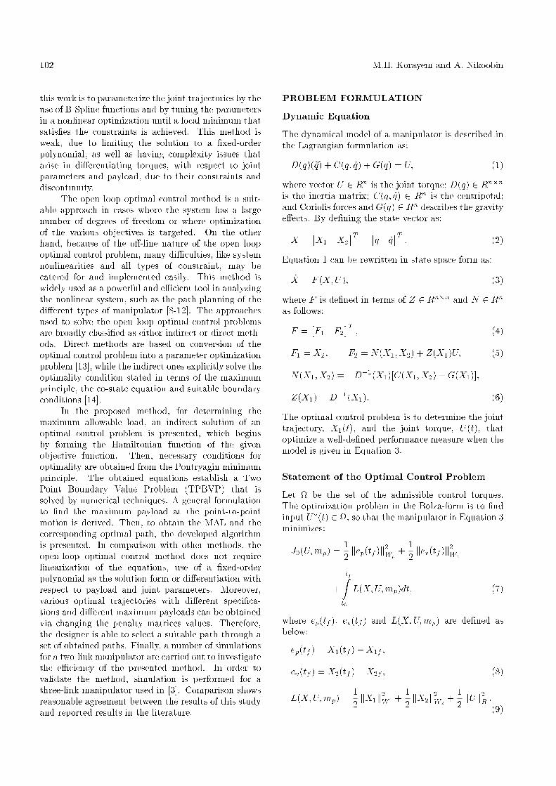
PROBLEM FORMULATION

Dynamic Equation

The dynamical model of a manipulator is described inthe Lagrangian formulation as:

D(q)(�q) + C(q; _q) +G(q) = U; (1)

where vector U 2 Rn is the joint torque; D(q) 2 Rn�nis the inertia matrix; C(q; _q) 2 Rn is the centripetal;and Coriolis forces and G(q) 2 Rn describes the gravitye�ects. By de�ning the state vector as:

X =�X1 X2

�T =�q _q

�T : (2)

Equation 1 can be rewritten in state space form as:

_X = F (X;U); (3)

where F is de�ned in terms of Z 2 Rn�n and N 2 Rnas follows:

F =�F1 F2

�T ; (4)

F1 = X2; F2 = N(X1; X2) + Z(X1)U; (5)

N(X1; X2) = �D�1(X1)[C(X1; X2) +G(X1)];

Z(X1) = D�1(X1): (6)

The optimal control problem is to determine the jointtrajectory, X1(t), and the joint torque, U(t), thatoptimize a well-de�ned performance measure when themodel is given in Equation 3.

Statement of the Optimal Control Problem

Let be the set of the admissible control torques.The optimization problem in the Bolza-form is to �ndinput U�(t) 2 , so that the manipulator in Equation 3minimizes:

J0(U;mp) =12kep(tf )k2Wp

+12kev(tf )k2Wv

+

tfZt0

L(X;U;mp)dt; (7)

where ep(tf ), ev(tf ) and L(X;U;mp) are de�ned asbelow:

ep(tf ) = X1(tf )�X1f ;

ev(tf ) = X2(tf )�X2f ; (8)

L(X;U;mp) =12kX1k2W1

+12kX2k2W2

+12kUk2R :

(9)

Formulation of Robots with Maximum Load Capacity 103

t0 and tf are known as the initial and �nal times,mp is the payload value carried by the manipulatorand the integrand, L(:), is a smooth, di�erentiablefunction in the arguments. kXk2K = XTKX is thegeneralized squared norm, Wp and We are symmetric,positive semi-de�nite (n � n) weighting matrices andW1, W2 and R are symmetric, positive de�nite (n�n)matrices. X1f and X2f are the desired values of theangular position and velocity of joints, respectively.The objective function speci�ed by Equations 7-9, isminimized over the entire duration of the motion. Theprimary goal expressed by the �rst and second termsin Equation 7 is to minimize the position and angularvelocity error at the �nal time. The �rst to thirdterms in Equation 9 represent the overall position,angular velocity and the total torque consumed duringthe motion, respectively. The designer can decide onthe relative importance among the angular positionand velocity, motion errors and control e�ort by thenumerical choice of W1, W2, Wp, Wv and R, which canalso be used to convert the dimensions of the terms toconsistent units. Initial and �nal boundary conditionscan be expressed as:

X1(0) = X10; X2(0) = X20;

X1(tf ) = X1f ; X2(tf ) = X2f ; (10)

which represent the angular position and velocity ofeach joint at the initial and �nal time. The permissiblebound of torque for each motor can be expressed as:

U =�U� � U � U+ : (11)

If U be a set of admissible control torque over the timeinterval, t 2 �t0 tf

�, for a speci�ed payload, the opti-

mal control problem is to obtain the U�(t) 2 U in sucha manner that the objective criterion in Equation 7is minimized, subject to motion equations, boundaryvalues and torque constraints given by Equations 3, 10and 11.

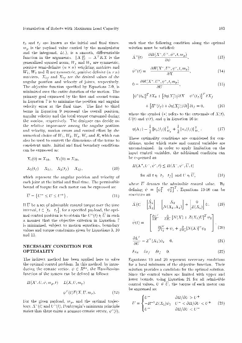
NECESSARY CONDITION FOROPTIMALITY

The indirect method has been applied here to solvethe optimal control problem. In this method, by intro-ducing the costate vector, 2 R2n, the Hamiltonianfunction of the system can be de�ned as follows:

H(X`; U; ;mp; t) = L(X;U;mp)

+ T (t)F (X;U;mp): (12)

For the given payload, mp, and the optimal trajec-tory, X�(t) and U�(t), Pontryagin's minimum principlestates that there exists a nonzero costate vector, �(t),

such that the following condition along the optimalsolution must be satis�ed:

_X�(t) =@H(X�; U�; �; t;mp)

@ ; (13)

_ �(t) = �@H(X�; U�; �; t;mp)@X

; (14)

0 =@H(X�; U�; �; t;mp)

@U; (15)

[ �(t0)]T �X0 +�@�(X�f )=@X � �(tf )

�T �Xf

+�H�(tf ) + @�(X�f )=@t

��tf = 0; (16)

where the symbol (�) refers to the extremals of X(t),U(t) and (t), and � in Equation 16 is:

�(Xf ) =12kep(tf )k2Wp

+12kev(tf )k2Wv

: (17)

These optimality conditions are considered for con-ditions, under which state and control variables areunconstrained. In order to apply limitation on theinput control variables, the additional condition canbe expressed as:

H(X�; U�; �; t) � H(X�; �; U; t)

for all t 2 �t0 tf�

and U 2 U; (18)

where U denotes the admissible control value. Byde�ning =

� T1 T2

�T , Equations 13-16 can berewritten as:

_X(t) =� _X1

_X2

�=�

X2N(X1; X2)

�+�

0Z(X1)

�U; (19)

_ (t) = �264@LT@X1

+ @@X1

[N(X) + Z(X1)U ]T 2

@LT@X2

+ 1 + @@X2

[N(X)]T 2

375 ;(20)

@LT

@U+ ZT (X1) 2 = 0; (21)

�x0 = �xf = �tf = 0: (22)

Equations 19 and 20 represent necessary conditionsfor a local minimum of the objective function. Theirsolution provides a candidate for the optimal solution.Since the control values are limited with upper andlower bounds, using Equation 21 for all admissiblecontrol values, U 2 U , the torque of each motor canbe expressed as:

U =

8><>:U+ @H=@U > U+

�R�1Z(X1) 2 U� < @H=@U < U+

U� @H=@U < U�(23)

104 M.H. Korayem and A. Nikoobin

The actuators that are used for medium and small sizemanipulators are permanent magnet D.C. motors. Thetorque speed characteristic of such D.C. motors may berepresented by the following linear equation [3]:

U+ = K1 �K2X2;

U� = �K1 �K2X2; (24)

where K1 =��s1 �s2 � � � �sn

�T , K2 = dig��s1=!m1 � � � �sn=!mn

�, �s is the stall torque and

!m is the maximum no load speed of the motor. The�nal and initial states and the traveling time are �xed;therefore, Equation 16 is reduced to Equation 22.Hence, the boundary conditions will be expressed asbelow:

X1(0) = X10; X2(0) = X20;

X1(tf ) = X1f ; X2(tf ) = X2f : (25)

The essential conditions in Equations 19 to 25 indicatethree relation sets:

(i) The dynamical model (Equations 19 and 20);(ii) The optimality condition (Equation 23);

(iii) The split boundary condition (Equations 22or 25). These conditions specify a TPBVP, whichcan be solved numerically.

An iterative algorithm for computing a solution toEquations 19 to 25 can be constructed by satisfying anytwo of the three foregoing conditions in each iteration.Then, the algorithm will be repeated on the thirdcondition awaiting the desired degree of accuracy. Thealgorithm used in this paper iterates over the boundaryvalues, while conditions (i) and (ii) are satis�ed ineach iteration. By replacing Equations 23 and 24 inEquations 19 and 20, a set of 4n ordinary di�erentialequations is established, which besides the 4n boundaryvalue condition given from Equation 25, forms a twopoint boundary value problem. The algorithm iterateson the initial values of the co-state until the �nal errorobtained from Equatoins 8 and 17 must be less thanthe desired accuracy, ". To put it another way, thefollowing relation must be satis�ed in the solution ofTPBVP:

12kX1(tf )�X1fk2Wp

+12kX2(tf )�X2fk2Wv

� ":(26)

Xf are the desired boundary condition at t = tf andX(tf ) are calculated states values at t = tf , per theco-state initial values obtained in the TPBVP solution.The relative importance of position and velocity errorsof each joint can be speci�ed, via choosing the com-ponents of Wp and Wv. Extremum values of motor

capacity, U+ and U�, are used for the maximumpayload, so that, by exceeding the payload of its ownmaximum, mp > mpmax, an excessive torque, which ismore than its permissible bounds, is required. But, thetorque constraints are satis�ed by Equations 23 and 24in each iteration and, as a result, the �nal error turnsinto a very large number. A criterion can be de�nedto determine the maximum payload by considering thisfact.

OPTIMAL PATH FOR MAXIMUMPAYLOAD

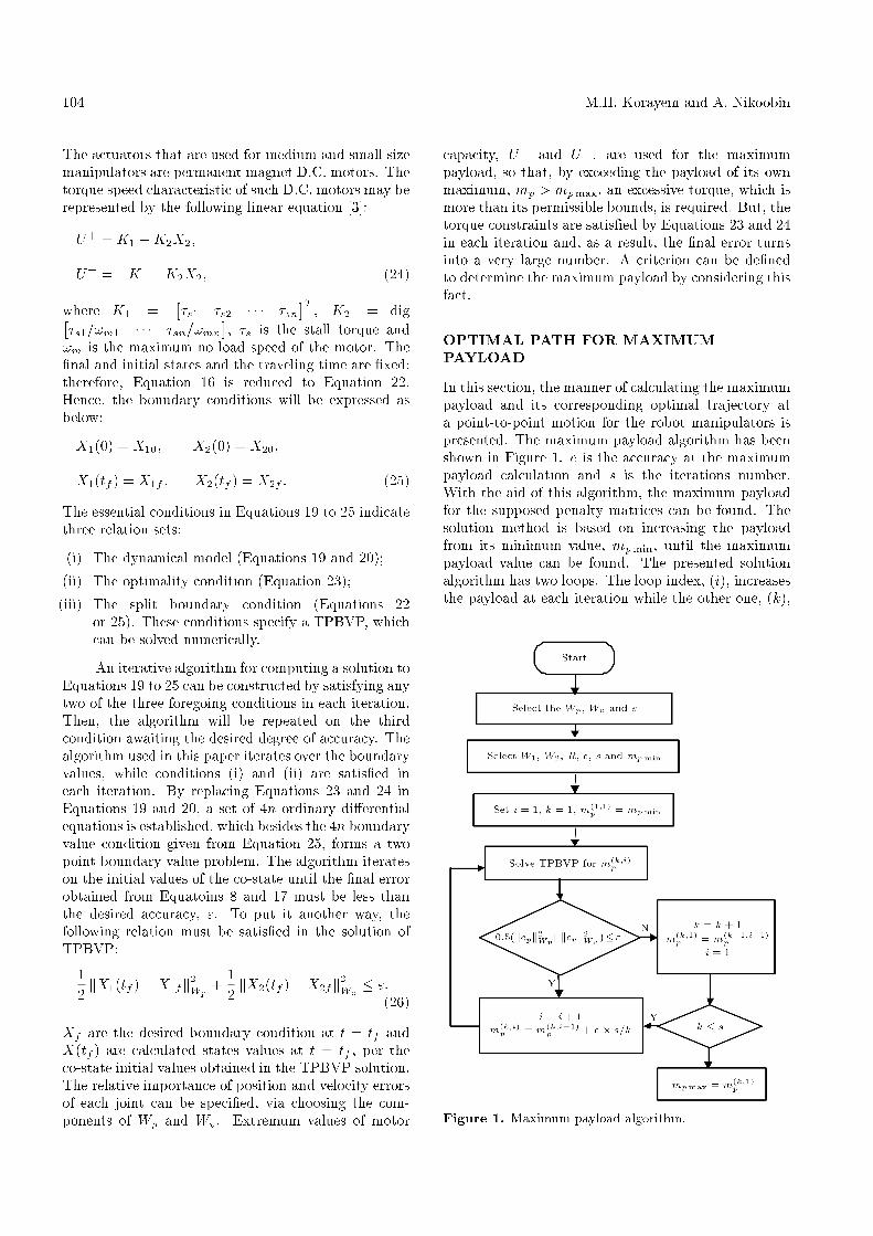
In this section, the manner of calculating the maximumpayload and its corresponding optimal trajectory ata point-to-point motion for the robot manipulators ispresented. The maximum payload algorithm has beenshown in Figure 1. e is the accuracy at the maximumpayload calculation and s is the iterations number.With the aid of this algorithm, the maximum payloadfor the supposed penalty matrices can be found. Thesolution method is based on increasing the payloadfrom its minimum value, mpmin, until the maximumpayload value can be found. The presented solutionalgorithm has two loops. The loop index, (i), increasesthe payload at each iteration while the other one, (k),

Figure 1. Maximum payload algorithm.

Formulation of Robots with Maximum Load Capacity 105

adjusts the jump interval. Therefore, the accuracyin payload calculation is guaranteed, as well as theapproaching rate to the �nal answer.

A TPBVP solution for mp � mpmax desiredaccuracy in the TPBVP solution is achievable, thus,Equation 26 is satis�ed. While, for mp > mpmax, theobtained error becomes considerably larger than ". Formpmax, the �nal error will be less than " and motorswork on their maximum capacity. Under this condition,carrying the payload more than mpmax is required,in order to apply torque to more than their limit,but, this is impossible, because the torque constraintsare satis�ed at each iteration in the TPBVP solution.Consequently, the error value becomes signi�cantlylarge. Using this fact, a criterion for maximum payloadcalculation is employed in the presented algorithm.

SIMULATION

In this section, simulations are performed for a two-linkand a three-link manipulator. Simulation for the two-link manipulator is carried out for two cases. In the�rst case, the maximum payload and its correspondingoptimal trajectory is determined for de�ned penaltymatrices. The second case is determination of themaximum payloads for the di�erent values of penaltymatrices and obtaining a set of optimal paths. Simula-tion for the three-link manipulator is performed for anarticulated robot used in [3], and the obtained resultsare compared with existing results. By comparison ofthe simulation results, the e�ciency of the proposedmethod will be investigated and the superiority of thismethod over the ILP method will be illustrated.

Simulation for a Two-Link Manipulator

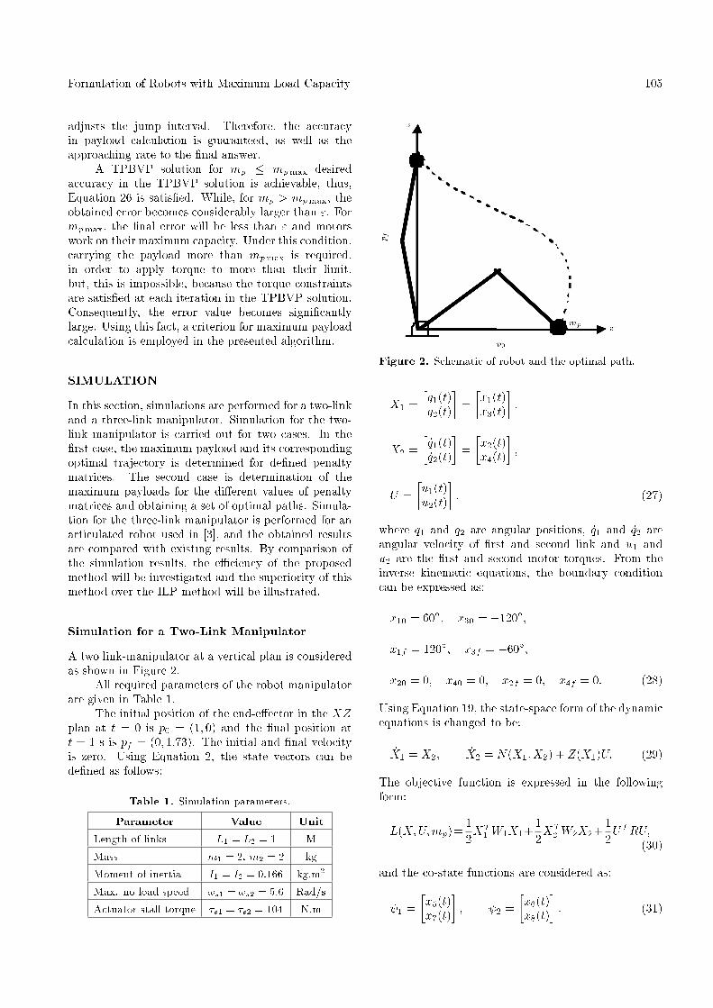
A two link-manipulator at a vertical plan is consideredas shown in Figure 2.

All required parameters of the robot manipulatorare given in Table 1.

The initial position of the end-e�ector in the XZplan at t = 0 is p0 = (1; 0) and the �nal position att = 1 s is pf = (0; 1:73). The initial and �nal velocityis zero. Using Equation 2, the state vectors can bede�ned as follows:

Table 1. Simulation parameters.

Parameter Value Unit

Length of links L1 = L2 = 1 M

Mass m1 = 2, m2 = 2 kg

Moment of inertia I1 = I2 = 0:166 kg.m2

Max. no load speed !s1 = !s2 = 5:6 Rad/s

Actuator stall torque �s1 = �s2 = 104 N.m

Figure 2. Schematic of robot and the optimal path.

X1 =�q1(t)q2(t)

�=�x1(t)x3(t)

�;

X2 =�

_q1(t)_q2(t)

�=�x2(t)x4(t)

�;

U =�u1(t)u2(t)

�; (27)

where q1 and q2 are angular positions, _q1 and _q2 areangular velocity of �rst and second link and u1 andu2 are the �rst and second motor torques. From theinverse kinematic equations, the boundary conditioncan be expressed as:

x10 = 60�; x30 = �120�;

x1f = 120�; x3f = �60�;

x20 = 0; x40 = 0; x2f = 0; x4f = 0: (28)

Using Equation 19, the state-space form of the dynamicequations is changed to be:

_X1 = X2; _X2 = N(X1; X2) + Z(X1)U: (29)

The objective function is expressed in the followingform:

L(X;U;mp)=12XT

1 W1X1+12XT

2 W2X2+12UTRU;

(30)

and the co-state functions are considered as:

1 =�x5(t)x7(t)

�; 2 =

�x6(t)x8(t)

�: (31)

106 M.H. Korayem and A. Nikoobin

Four equations concerned with co-state function areobtained from Equation 20 as follows:

_ 1 = �W1X1 � @X1

[N(X) + ZU ]T 2;

_ 2 = �W2X2 � 1 � @X2

[N(X)]T 2: (32)

The control values from Equations 21 and 23 can bewritten as:

U =

8><>:U+ �R�1Z(X1) 2 > U+

�R�1Z(X1) 2 U�<�R�1Z(X1) 2<U+

U� �R�1Z(X1) 2 < U� (33)

U+ and U� are substituted from Equation 24 into thisequation, so that the control value, U , is calculatedin terms of the states, co-states and penalty matricesvalues. By substituting Equation 33 into Equations 29and 32, eight nonlinear ordinary di�erential equationswill be obtained. For the sake of massive calculation,deriving the equations in details are not presented.Eight equations given in Equations 29 and 32, witheight boundary conditions given in Equation 28, con-struct a TPBVP. This problem can be solved using theBVP4C command in MATLAB r .

Simulation for Maximum Payload Trajectory

The accuracy matrices and penalty matrices are con-sidered to be Wp = Wv = diag(1) and W1 = W2 = [0],R = diag(1e�5). The desired accuracy in the TPBVPsolution and payload calculation is considered as: " =0:001 and e = 0:01. Using the obtained equations fromthe previous section and on the basis of the presentedalgorithm in Figure 1, mp increases from mpmin tompmax. A simulation for the range of mp, given inTable 2, is performed. The maximum payload for thesevalues of penalty matrices is found to be 5.53 kg.

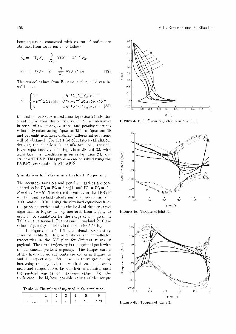
In Figures 3 to 5, 1-6 labels denote six existingcases of Table 2. Figure 3 shows the end-e�ectortrajectories in the XZ plan for di�erent values ofpayload. The sixth trajectory is the optimal path withthe maximum payload capacity. The torque curvesof the �rst and second joints are shown in Figure 4aand 4b, repectively. As shown in these graphs, byincreasing the payload, the required torque becomesmore and torque curves lay on their own limits, untilthe payload reaches its maximum value. For thesixth case, the highest possible values of the torque

Table 2. The values of mp used in the simulation.

i 1 2 3 4 5 6

mpmax 0.1 2 4 5 5.3 5.53

Figure 3. End-e�ector trajectories in XZ plan.

Figure 4a. Torques of joints 1.

Figure 4b. Torques of joints 2.

Formulation of Robots with Maximum Load Capacity 107

Figure 5a. Angular velocities of joints 1.

Figure 5b. Angular velocities of joints 2.

are applied and an increase in the payload of morethan 5.53 kg is required to apply the torque beyondthe limits. The angular velocities of the �rst andsecond joints for di�erent values of payload are givenin Figures 5. It can be seen that increasing the payloadleads to more velocity in the joints.

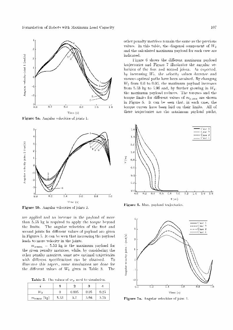
mpmax = 5:53 kg is the maximum payload forthe given penalty matrices, while, by considering theother penalty matrices, some new optimal trajectorieswith di�erent speci�cations can be obtained. Toillustrate this aspect, some simulations are done forthe di�erent values of W2 given in Table 3. The

Table 3. The values of mp used to simulation.

i 1 2 3 4

W2 0 0.005 0.05 0.25

mpmax (kg) 5.53 5.7 5.96 5.75

other penalty matrices remain the same as the previousvalues. In this table, the diagonal component of W2and the calculated maximum payload for each case areindicated.

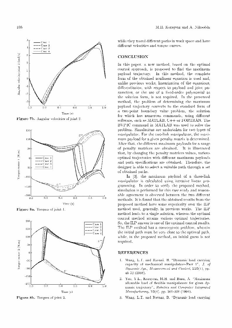
Figure 6 shows the di�erent maximum payloadtrajectories and Figure 7 illustrates the angular ve-locities of the �rst and second joints. As expected,by increasing W2, the velocity values decrease andvarious optimal paths have been attained. By changingW2 from 0.0 to 0.05, the maximum payload increasesfrom 5.53 kg to 5.96 and, by further growing in W2,the maximum payload reduces. The torques and thetorque limits for di�erent values of mpmax are shownin Figure 8. It can be seen that, in each case, thetorque curves have been laid on their limits. All ofthese trajectories are the maximum payload paths,

Figure 6. Max. payload trajectories.

Figure 7a. Angular velocities of joint 1.

108 M.H. Korayem and A. Nikoobin

Figure 7b. Angular velocities of joint 2.

Figure 8a. Torques of joint 1.

Figure 8b. Torques of joint 2.

while they travel di�erent paths in work space and havedi�erent velocities and torque curves.

CONCLUSION

In this paper, a new method, based on the optimalcontrol approach, is proposed to �nd the maximumpayload trajectory. In this method, the completeform of the obtained nonlinear equation is used and,unlike previous works, linearization of the equations,di�erentiation, with respect to payload and joint pa-rameters, or the use of a �xed-order polynomial asthe solution form, is not required. In the presentedmethod, the problem of determining the maximumpayload trajectory converts to the standard form ofa two-point boundary value problem, the solutionfor which has numerous commands, using di�erentsoftware, such as MATLAB, C++ or FORTRAN. TheBVP4C command in MATLAB was used to solve theproblem. Simulations are undertaken for two types ofmanipulator. For the two-link manipulator, the maxi-mum payload for a given penalty matrix is determined.After that, the di�erent maximum payloads for a rangeof penalty matrices are obtained. It is illustratedthat, by changing the penalty matrices values, variousoptimal trajectories with di�erent maximum payloadsand path speci�cations are obtained. Therefore, thedesigner is able to select a suitable path through a setof obtained paths.

In [3], the maximum payload of a three-linkmanipulator is calculated using iterative linear pro-gramming. In order to verify the proposed method,simulation is performed for this case study and reason-able agreement is observed between the two di�erentmethods. It is found that the obtained results from theproposed method have some superiority over the ILPmethod used, generally, in previous works. The ILPmethod leads to a single solution, whereas the optimalcontrol method attains various optimal trajectories.So, the ILP answer is one of the optimal control results.The ILP method has a convergence problem, whereinthe initial path must be very close to the optimal path,while, in the proposed method, an initial guess is notrequired.

REFERENCES

1. Wang, L.T. and Ravani, B. \Dynamic load carryingcapacity of mechanical manipulators-Part 1", J. ofDynamic Sys., Measurement and Control, 110(1), pp.46-52 (1988).

2. Yao, Y.L., Korayem, M.H. and Basu, A. \Maximumallowable load of exible manipulators for given dy-namic trajectory", Robotics and Computer IntegratedManufacturing, 10(4), pp. 301-308 (1994).

3. Wang, L.T. and Ravani, B. \Dynamic load carrying

Formulation of Robots with Maximum Load Capacity 109

capacity of mechanical manipulators-Part 2", J. ofDynamic Sys., Measurement and Control, 110(1), pp.53-61 (1988).

4. Korayem, M.H. and Ghariblu, H. \Maximum allowableload of mobile manipulator for two given end points ofend-e�ector", Int. J. of Adv. Manuf. Technol., 24(10),pp. 743-751 (2004).

5. Korayem, M.H. and Gariblu, H. \Analysis of wheeledmobile exible manipulator dynamic motions withmaximum load carrying capacities", Robotics and Au-tonomous Systems, 48(3), pp. 63-76 (2004).

6. Gariblu, H. and Korayem, M.H. \Trajectory optimiza-tion of exible mobile manipulators", Robotica, 24(3),pp. 333-335 (2006).

7. Wang, C-Y.E., Timoszyk, W.K. and Bobrow, J.E.\Payload maximization for open chained manipulator:Finding motions for a Puma 762 robot", IEEE Trans-actions on Robotics and Automation, 17(2), pp. 218-224 (2001).

8. Koivo, A.J. and Arnautovic, S.H. \Dynamic optimumcontrol of redundant manipulators", Proc. IEEE Int.Conf. on Robotics and Automation, pp. 466-471 (1991).

9. Mohri, A., Furuno, S., Iwamura, M. and Yamamoto,M. \Sub-optimal trajectory planning of mobile ma-nipulator", Proc. IEEE Int. Conf. on Robotics andAutomation, pp. 1271-1276 (2001).

10. Kelly, A. and Nagy, B. \Reactive nonholonomic tra-jectory generation via parametric optimal control",International Journal of Robotics Research, 22(8), pp.583-601 (2003).

11. Furuno, S., Yamamoto, M. and Mohri, A. \Trajectoryplanning of mobile manipulator with stability con-siderations", Proc. IEEE Int. Conf. on Robotics andAutomation, Taiwan, pp. 3403-3408 (2003).

12. Wilson, D.G., Robinett, R.D. and Eisler, G.R. \Dis-crete dynamic programming for optimized path plan-ning of exible robots", Proc. IEEE Int. Conf. onlntelligent Robots and Systems, Japan (2004).

13. Hull, D.G. \Conversion of optimal control problemsinto parameter optimization problems", J. of Guid-ance, Control and Dynamics, 20(1), pp. 57-60 (1997).

14. Kirk, D.E., Optimal Control Theory; an Introduction,Prentice-Hall Inc. (1970).