Foundation Engineering Prof. Dr N.K. Samadhiya …textofvideo.nptel.ac.in/105107120/lec4.pdf · have discussed the Terzaghi bearing capacity equation where half bearing capacity

Foundation Engineering

Prof. Dr N.K. Samadhiya

Department of Civil Engineering

Indian Institute of Technology Roorkee

Module - 01

Lecture - 04

Shallow Foundation

So, friends I again welcome you for this lecture series on shallow foundation. So, far we

have discussed the Terzaghi bearing capacity equation where half bearing capacity

equation considering all these say factors inclination factors and dap factors. And the

modifications in the bearing capacity, parameter, parameters bearing capacity factors like

Nc Nq N gamma we have also seen the Skempton, bearing capacity parameters for the

cohesive soils. And we have discussed several solved problems so, as to use how to use,

so as to make use of these equations for various shapes and to determine the unknown

parameters. Now, the parameters which are required are the strength parameters and the

bearing capacity factors.

Now, a strength parameters c and phi can be determined in laboratory by conducting

laboratory test like triaxial test or may be directional test or sometimes unconfirmed

compression test. The Nq N gamma and Nc parameters are the functions of phi and by

using equations those developed by either Mayer Half or Terzaghi or Henson or Wersik

we can find out those parameters and substitute in the bearing capacity equation. We

have also discussed the procedure which is suggested in IS 6 4 0 3 1981 which is nothing

but the procedure given by Brinch Hansen and in which the effect of water table

correction is also taken into account.

Now, there are few methods which are available to determine ultimate bearing capacity

of foundations based on the field test. So, in field, we normally conduct plate load test

extended validation test and if required for a special cases and if the requirement is

necessary then we also conduct static cone penetration test. And then from those test we

also determine the parameters strength parameters or sometimes be directly determine

parameter N gamma and from N gamma we find out phi and then other parameters are

determined.

(Refer Slide Time: 03:05)

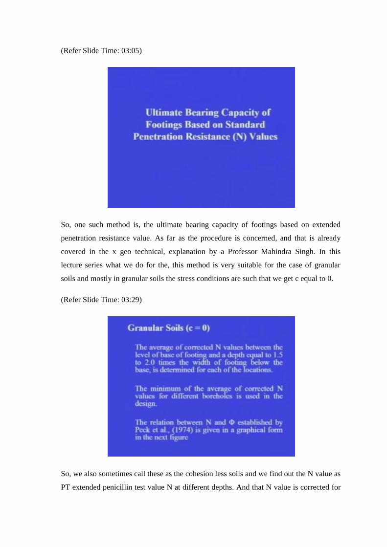
So, one such method is, the ultimate bearing capacity of footings based on extended

penetration resistance value. As far as the procedure is concerned, and that is already

covered in the x geo technical, explanation by a Professor Mahindra Singh. In this

lecture series what we do for the, this method is very suitable for the case of granular

soils and mostly in granular soils the stress conditions are such that we get c equal to 0.


So, we also sometimes call these as the cohesion less soils and we find out the N value as

PT extended penicillin test value N at different depths. And that N value is corrected for

overburden and dilatancy. Normally the corrected N values between the level of base of

footing and a depth equal to 1.5 to 2 times the width of footing below the base is

determined for each locations. And as we know that these standard penicillin tests are

conducted in the boreholes and we advanced borehole may be up to 12 meter 15 meter

and at each 1.5 meter depth we conduct this test.

So, these values are observed and observed values then corrected for overburden or

dilatancy wherever required depending upon the water table or the type of soil. The

minimum of the average of corrected N values for different boreholes is used in the

design. Now, in our particular project normally depending upon the requirement 4 5

boreholes at least are conducted and the average corrected values are determined for a

depth equal to 1.5 to 2 times the width of the footing below the base and the minimum of

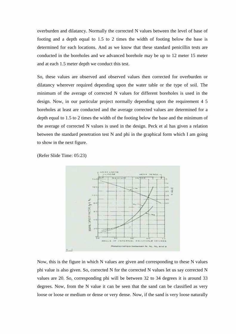
the average of corrected N values is used in the design. Peck et al has given a relation

between the standard penetration test N and phi in the graphical form which I am going

to show in the next figure.


Now, this is the figure in which N values are given and corresponding to these N values

phi value is also given. So, corrected N for the corrected N values let us say corrected N

values are 20. So, corresponding phi will be between 32 to 34 degrees it is around 33

degrees. Now, from the N value it can be seen that the sand can be classified as very

loose or loose or medium or dense or very dense. Now, if the sand is very loose naturally

there will be local shear failure possibility of local shear failure is more than in the case

of very dense sand there is a possibility of general shear failure.

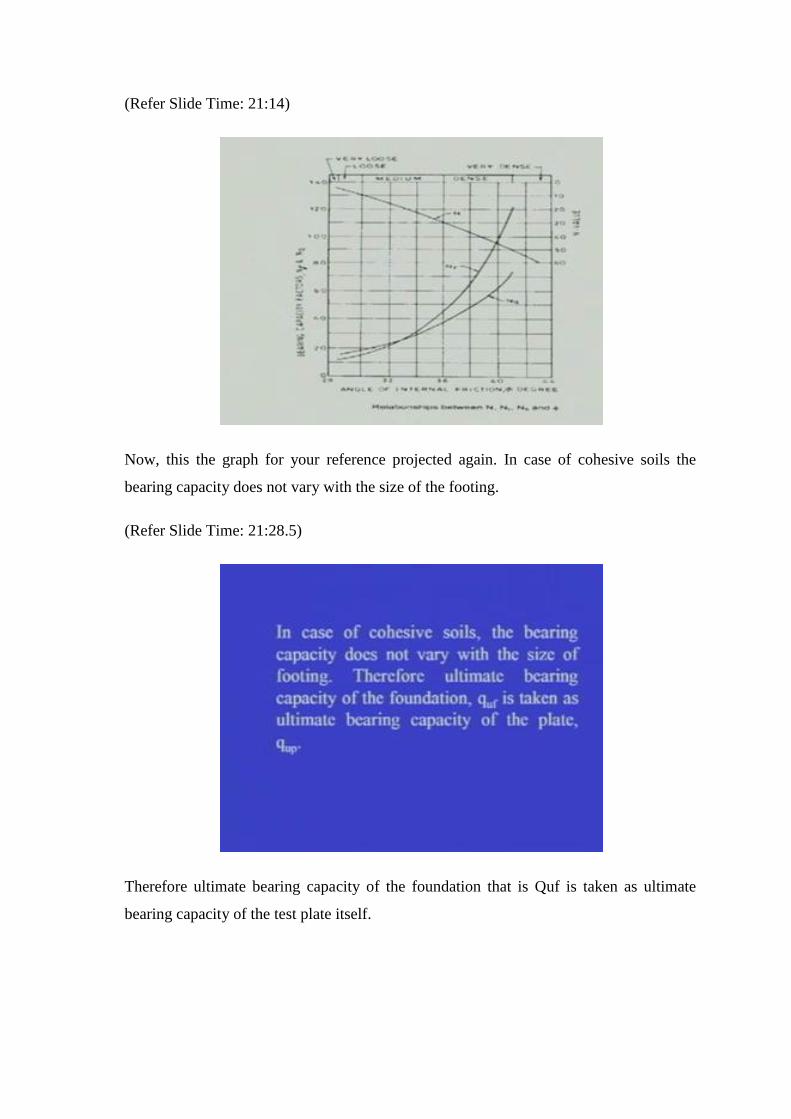
So, either we take phi value from here or then Nc Nq N gamma parameters can be

determined from the Terzaghi table or directly from this chart in which the intermede the

values are covered from local shear failure case to general shear failure case this is the

chart given by Peck et al. So, here for the given value of N we can directly find out what

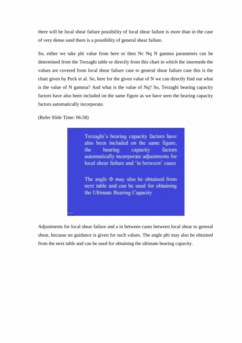
is the value of N gamma? And what is the value of Nq? So, Terzaghi bearing capacity

factors have also been included on the same figure as we have seen the bearing capacity

factors automatically incorporate.


Adjustments for local shear failure and a in between cases between local shear to general

shear, because no guidance is given for such values. The angle phi may also be obtained

from the next table and can be used for obtaining the ultimate bearing capacity.


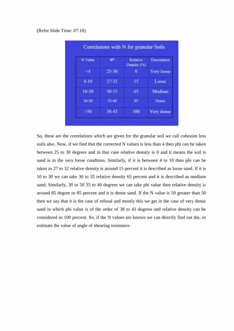
So, these are the correlations which are given for the granular soil we call cohesion less

soils also. Now, if we find that the corrected N values is less than 4 then phi can be taken

between 25 to 30 degrees and in that case relative density is 0 and it means the soil is

sand is in the very loose condition. Similarly, if it is between 4 to 10 then phi can be

taken as 27 to 32 relative density is around 15 percent it is described as loose sand. If it is

10 to 30 we can take 30 to 35 relative density 65 percent and it is described as medium

sand. Similarly, 30 to 50 35 to 40 degrees we can take phi value then relative density is

around 85 degree or 85 percent and it is dense sand. If the N value is 50 greater than 50

then we say that it is the case of refusal and mostly this we get in the case of very dense

sand in which phi value is of the order of 38 to 43 degrees and relative density can be

considered as 100 percent. So, if the N values are known we can directly find out the, or

estimate the value of angle of shearing resistance.


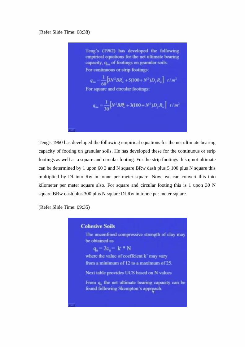
Teng's 1960 has developed the following empirical equations for the net ultimate bearing

capacity of footing on granular soils. He has developed these for the continuous or strip

footings as well as a square and circular footing. For the strip footings this q not ultimate

can be determined by 1 upon 60 3 and N square BRw dash plus 5 100 plus N square this

multiplied by Df into Rw in tonne per meter square. Now, we can convert this into

kilometer per meter square also. For square and circular footing this is 1 upon 30 N

square BRw dash plus 300 plus N square Df Rw in tonne per meter square.


The N values are also related to the unconfined compressive strength as well as. From

unconfined compressive strength we can determine the undrained cohegen which can be

used in the calculation of bearing capacity. The unconfined compressive strength of clay

may be obtained as qu equal to this is the undrained or unconfined compressive strength.

Sometimes this undrained is, because if we conduct unconsolidated undrained test in

triaxial then this is the strength in undrained condition for the fully saturated soil and that

becomes equal to 2 times undrained cohegen and it is equal to K dash into N where the

value of coefficient k dash may vary. It is from a minimum of 12 to a maximum value of

25. So, in next tables table provides UCS based on N value. Now, from qu the net

ultimate bearing capacity can be found following the Skempton’s approach.


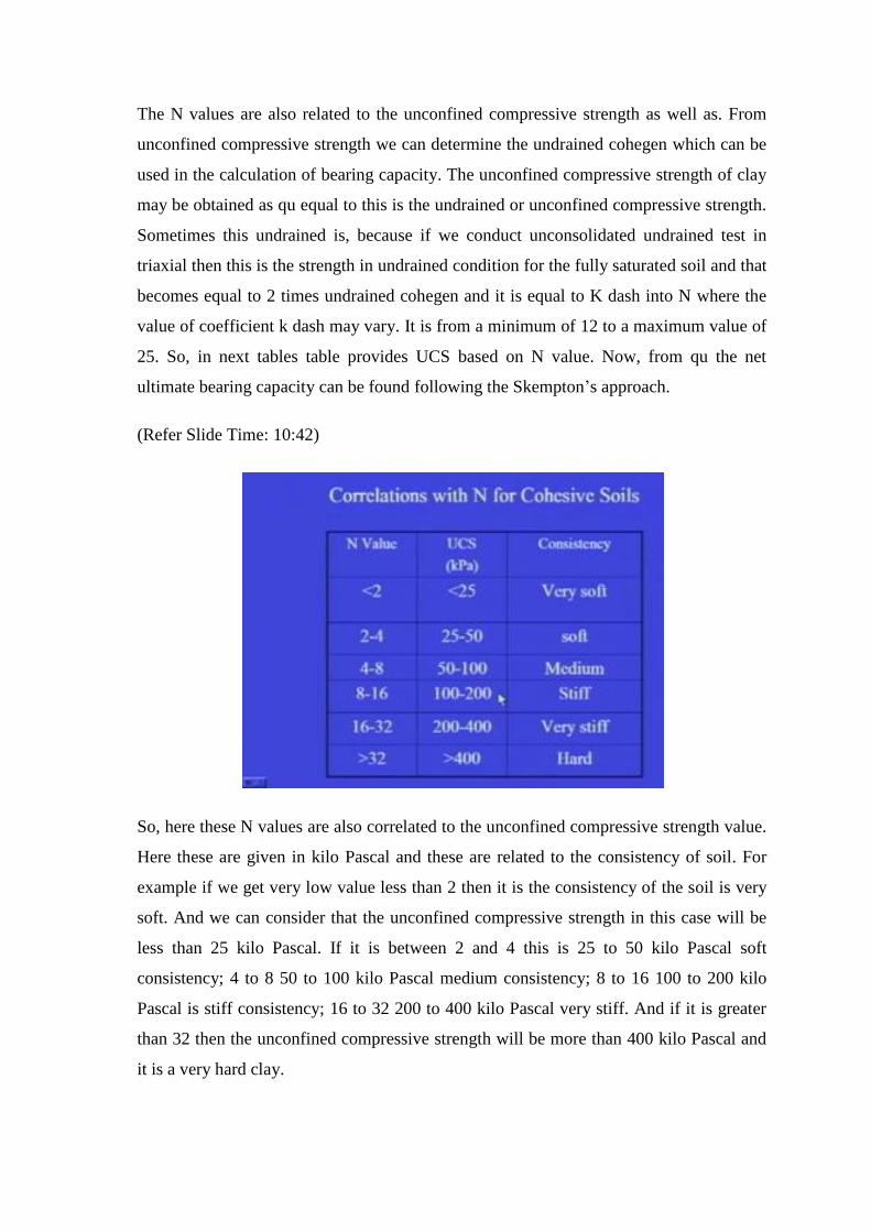
So, here these N values are also correlated to the unconfined compressive strength value.

Here these are given in kilo Pascal and these are related to the consistency of soil. For

example if we get very low value less than 2 then it is the consistency of the soil is very

soft. And we can consider that the unconfined compressive strength in this case will be

less than 25 kilo Pascal. If it is between 2 and 4 this is 25 to 50 kilo Pascal soft

consistency; 4 to 8 50 to 100 kilo Pascal medium consistency; 8 to 16 100 to 200 kilo

Pascal is stiff consistency; 16 to 32 200 to 400 kilo Pascal very stiff. And if it is greater

than 32 then the unconfined compressive strength will be more than 400 kilo Pascal and

it is a very hard clay.


Another test which we normally use in the case of again granular soil which is most

suitable for granular soil we that test is plate load test. And from the plate load test data

we can find out ultimate bearing capacity of footings.


Now, in the plate load test or test plate, square or circular in shape, is used as a model for

the prototype foundation. The plate is placed at the proposed level of foundation and is

subjected to incremental loading. Settlement at each increment of loading is measured

and a load settlement curve is plotted. The bearing capacity of the plate is determined

from the plate load settlement curve, and the test procedure is explained in IS 1888 1982.


Briefly I will discuss the procedure here and although the procedure must have been

describe by Professor Mahindra Singh. So, briefly I am going to discuss this procedure

which is explained below. Rough mild steel plates 30 centimeter 60 centimeter or 75

centimeter in size, square in shape, are used. The smaller sizes are used in dense or stiff

clays and larger sizes in loose or soft soils. A pit of dimensions not less than 5 times the

width of the plate is excavated up to the proposed depth of foundation. And the test plate

is seated at the center over a fine sand layer of maximum thickness 5 millimeter.


If the water table is above the level of the test pit, water is carefully pumped out to bring

down the water table to the level of foundation before seating the test plate. Loads and

the test plate may be applied by gravity loading or by reaction loading. For gravity

loading a platform is constructed on a vertical column resting on the plate. Loading on

the plate is done by placing weighted sand bags on the platform in reaction loading. The

load is applied through proving ring and hydraulic jack by taking reaction against of

fixed support. Next figure shows the plate load test set up.


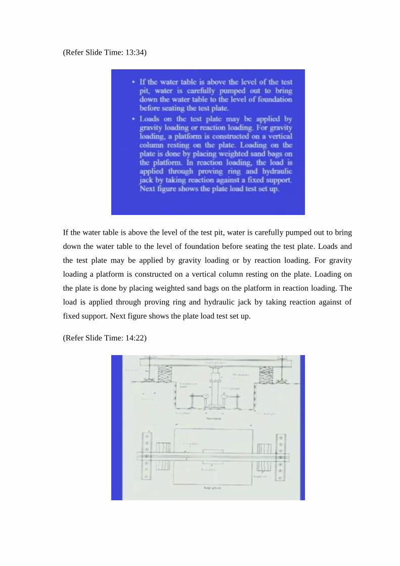
Now, this particular figure, in this particular figure you can see that there is an

excavation of the 5 times the width of the test plate. So, this is the test plate and 5 times

the width the depth of the foundation is up to the level proposed level of foundation. Test

plate is placed and over that column is there and from this column which is the extension

pipe. The load is applied by hydraulic jack and the reaction is taken from these steel

guarders while these guarders may be faced by anchors. So, the reaction is taken by the

soil or the anchoring axial. Now, these are like ISHB or ISMB channels deformation of

this plate due to the loading is determined or measured by the deformation dial gauges 4

dial gauges are used or sometimes at least 2 dial gauges are placed diametrically opposite

to the test plate. The plan of this setup is shown in this figure. Now, these are anchors are

fixed by nut and bold arrangement here.


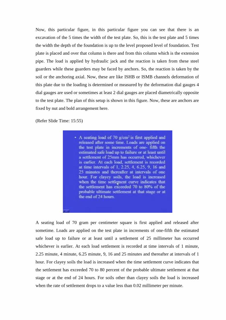
A seating load of 70 gram per centimeter square is first applied and released after

sometime. Loads are applied on the test plate in increments of one-fifth the estimated

safe load up to failure or at least until a settlement of 25 millimeter has occurred

whichever is earlier. At each load settlement is recorded at time intervals of 1 minute,

2.25 minute, 4 minute, 6.25 minute, 9, 16 and 25 minutes and thereafter at intervals of 1

hour. For clayey soils the load is increased when the time settlement curve indicates that

the settlement has exceeded 70 to 80 percent of the probable ultimate settlement at that

stage or at the end of 24 hours. For soils other than clayey soils the load is increased

when the rate of settlement drops to a value less than 0.02 millimeter per minute.


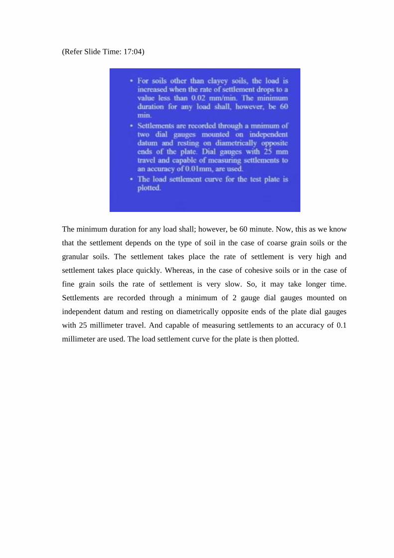
The minimum duration for any load shall; however, be 60 minute. Now, this as we know

that the settlement depends on the type of soil in the case of coarse grain soils or the

granular soils. The settlement takes place the rate of settlement is very high and

settlement takes place quickly. Whereas, in the case of cohesive soils or in the case of

fine grain soils the rate of settlement is very slow. So, it may take longer time.

Settlements are recorded through a minimum of 2 gauge dial gauges mounted on

independent datum and resting on diametrically opposite ends of the plate dial gauges

with 25 millimeter travel. And capable of measuring settlements to an accuracy of 0.1

millimeter are used. The load settlement curve for the plate is then plotted.


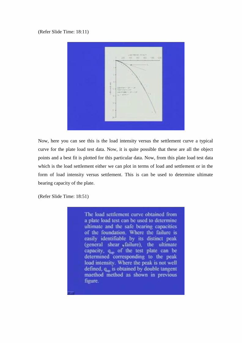
Now, here you can see this is the load intensity versus the settlement curve a typical

curve for the plate load test data. Now, it is quite possible that these are all the object

points and a best fit is plotted for this particular data. Now, from this plate load test data

which is the load settlement either we can plot in terms of load and settlement or in the

form of load intensity versus settlement. This is can be used to determine ultimate

bearing capacity of the plate.


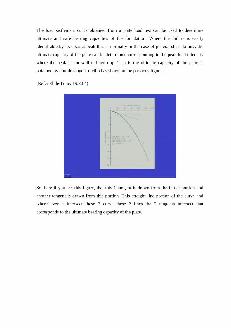
The load settlement curve obtained from a plate load test can be used to determine

ultimate and safe bearing capacities of the foundation. Where the failure is easily

identifiable by its distinct peak that is normally in the case of general shear failure, the

ultimate capacity of the plate can be determined corresponding to the peak load intensity

where the peak is not well defined qup. That is the ultimate capacity of the plate is

obtained by double tangent method as shown in the previous figure.

(Refer Slide Time: 19:30.4)

So, here if you see this figure, that this 1 tangent is drawn from the initial portion and

another tangent is drawn from this portion. This straight line portion of the curve and

where ever it intersect these 2 curve these 2 lines the 2 tangents intersect that

corresponds to the ultimate bearing capacity of the plate.


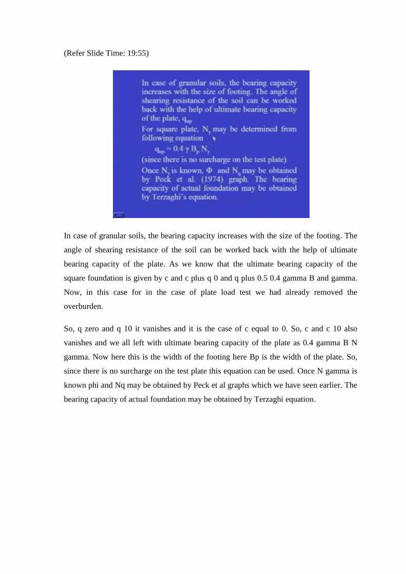
In case of granular soils, the bearing capacity increases with the size of the footing. The

angle of shearing resistance of the soil can be worked back with the help of ultimate

bearing capacity of the plate. As we know that the ultimate bearing capacity of the

square foundation is given by c and c plus q 0 and q plus 0.5 0.4 gamma B and gamma.

Now, in this case for in the case of plate load test we had already removed the

overburden.

So, q zero and q 10 it vanishes and it is the case of c equal to 0. So, c and c 10 also

vanishes and we all left with ultimate bearing capacity of the plate as 0.4 gamma B N

gamma. Now here this is the width of the footing here Bp is the width of the plate. So,

since there is no surcharge on the test plate this equation can be used. Once N gamma is

known phi and Nq may be obtained by Peck et al graphs which we have seen earlier. The

bearing capacity of actual foundation may be obtained by Terzaghi equation.


Now, this the graph for your reference projected again. In case of cohesive soils the

bearing capacity does not vary with the size of the footing.

(Refer Slide Time: 21:28.5)

Therefore ultimate bearing capacity of the foundation that is Quf is taken as ultimate

bearing capacity of the test plate itself.


Results of plate load test need to be interpreted with caution. Some of the important

considerations are given as follows: In no case shall a test plate smaller in width than 30

centimeter be used. Because experimental evidence has indicated that the load settlement

behaviour of the soil is qualitatively different for smaller widths of the test plate

compared to that of larger widths.


It has been found that in the case of granular soils, the settlement of a foundation cannot

exceed about 4 times the settlement of a plate of 30 centimeter width, howsoever large it

may be.


If the soil at the site is not homogeneous up to a large depth relative to the size of the

foundation, the plate load test may lead to misleading results. For example, if the upper

stratum of stratified soil is a strong soil like dense sand and the lower stratum is a weak

soil like soft clay in such a situation. The load test results reflect the load settlement

characteristics of the stronger stratum, but does not give any indication of the settlement

behaviour of the poorer soil below.


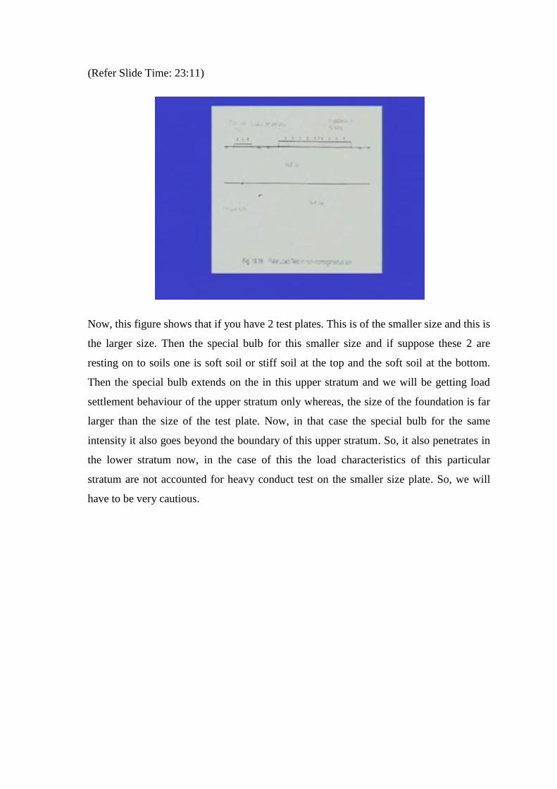
Now, this figure shows that if you have 2 test plates. This is of the smaller size and this is

the larger size. Then the special bulb for this smaller size and if suppose these 2 are

resting on to soils one is soft soil or stiff soil at the top and the soft soil at the bottom.

Then the special bulb extends on the in this upper stratum and we will be getting load

settlement behaviour of the upper stratum only whereas, the size of the foundation is far

larger than the size of the test plate. Now, in that case the special bulb for the same

intensity it also goes beyond the boundary of this upper stratum. So, it also penetrates in

the lower stratum now, in the case of this the load characteristics of this particular

stratum are not accounted for heavy conduct test on the smaller size plate. So, we will

have to be very cautious.


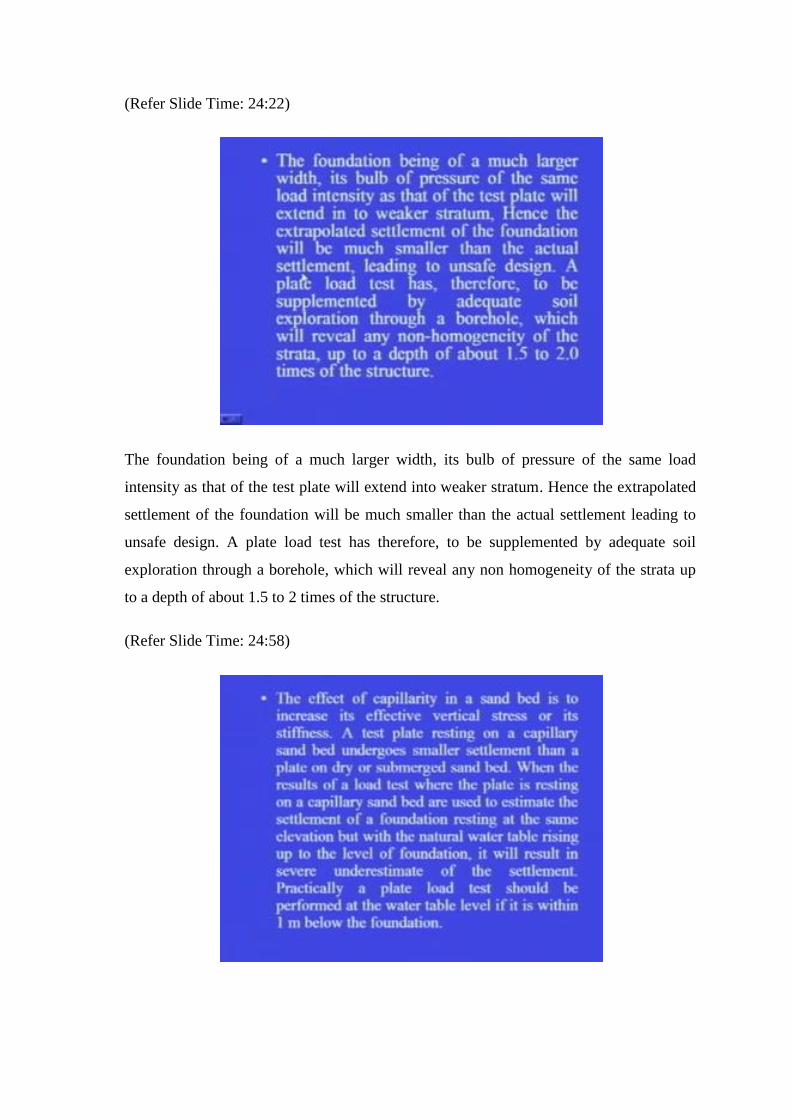
The foundation being of a much larger width, its bulb of pressure of the same load

intensity as that of the test plate will extend into weaker stratum. Hence the extrapolated

settlement of the foundation will be much smaller than the actual settlement leading to

unsafe design. A plate load test has therefore, to be supplemented by adequate soil

exploration through a borehole, which will reveal any non homogeneity of the strata up

to a depth of about 1.5 to 2 times of the structure.


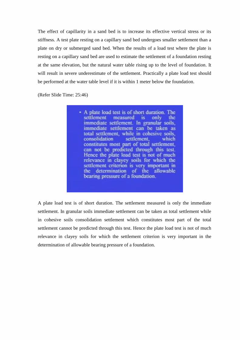
The effect of capillarity in a sand bed is to increase its effective vertical stress or its

stiffness. A test plate resting on a capillary sand bed undergoes smaller settlement than a

plate on dry or submerged sand bed. When the results of a load test where the plate is

resting on a capillary sand bed are used to estimate the settlement of a foundation resting

at the same elevation, but the natural water table rising up to the level of foundation. It

will result in severe underestimate of the settlement. Practically a plate load test should

be performed at the water table level if it is within 1 meter below the foundation.


A plate load test is of short duration. The settlement measured is only the immediate

settlement. In granular soils immediate settlement can be taken as total settlement while

in cohesive soils consolidation settlement which constitutes most part of the total

settlement cannot be predicted through this test. Hence the plate load test is not of much

relevance in clayey soils for which the settlement criterion is very important in the

determination of allowable bearing pressure of a foundation.


So, to very cautious when we interpret the plate load test data. Now, another test which is

preferred is the static cone penetration test by which we find out CPT values termed as

qc values and ultimate bearing capacity of footing can be determined from these qc

values.


For the granular soil, as per Schmertmann the bearing capacity factor N gamma for use

in the Terzaghi’s bearing capacity equation can be determined as follows. N gamma can

be taken as 1.25 times qc where qc is the cone point resistance in kg per centimeter

square average over a depth equal to 1.5 to 2 times width below the foundation. With the

known values of N gamma phi and bearing capacity factor nq and hence ultimate bearing

capacity can be determined.


In the case of clay soils, the undrained shear strength cu under phi equal to 0 condition

may be related to the static cone point resistance qc as qc equal to Nk cu plus p 0. Where

Nk is the cone factor which is approximately 20 for both normally and over consolidated

clays and p 0 is equal to the total overburden pressure represented as sigma 0 also.


So, ultimate bearing capacity of foundations can also be determined from the field test.

And the in order to design the foundation, we also need to know the settlement of

shallow foundation. Because the design criteria say that the bearing capacity of the

foundations should be sufficient. So, that there is no shear failure of the soil and the

settlement should be within permissible limits. So, I am going to discuss now, to

determine settlement of shallow foundations. Now, first of all let us see what are the

effects of settlement on the structure.


If the structure has as a whole settles uniformly into the ground there will not be any

detrimental effect on the structure. The only effect it can have is on the service lines such

as water and sanitary pipe lines which can break if settlement is considerable.


Several structures in Mexico City have undergone enormous settlements of the order of

as large as 2 meter, but are still functional, because the settlement has been uniform.

Such uniform settlement is possible only if the subsoil is homogeneous and the load

distribution is uniform.


However, the differential settlement should not exceed the permissible limits. A structure

is said to undergo differential settlement if onw of its part settles more than the other.

Angular distortion is the ratio of the differential settlement between 2 columns to the

spacing between them.


Tilt occurs when the entire structure rotates as a consequence of a non-uniform

settlement. A classical example of tilt is the leaning tower of Pisa. Definition of

differential settlement for framed and load bearing wall structures are shown in the next

figure which are given by Burland and Worth 1974.


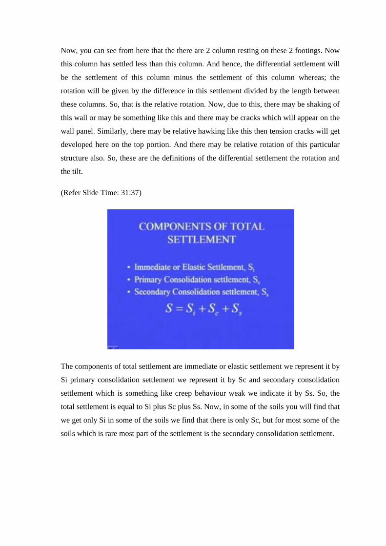
Now, you can see from here that the there are 2 column resting on these 2 footings. Now

this column has settled less than this column. And hence, the differential settlement will

be the settlement of this column minus the settlement of this column whereas; the

rotation will be given by the difference in this settlement divided by the length between

these columns. So, that is the relative rotation. Now, due to this, there may be shaking of

this wall or may be something like this and there may be cracks which will appear on the

wall panel. Similarly, there may be relative hawking like this then tension cracks will get

developed here on the top portion. And there may be relative rotation of this particular

structure also. So, these are the definitions of the differential settlement the rotation and

the tilt.


The components of total settlement are immediate or elastic settlement we represent it by

Si primary consolidation settlement we represent it by Sc and secondary consolidation

settlement which is something like creep behaviour weak we indicate it by Ss. So, the

total settlement is equal to Si plus Sc plus Ss. Now, in some of the soils you will find that

we get only Si in some of the soils we find that there is only Sc, but for most some of the

soils which is rare most part of the settlement is the secondary consolidation settlement.


Immediate settlement is that part of total settlement which takes place immediately that

is during a short time after the application of loading. In a clay soil it is also known as

distortion settlement and is due to change in shape of soil without a change in volume or

water content. In granular soils immediate settlement accounts virtually for the entire

settlement there is very less consolidation settlement. Immediate settlement is compared

is computed using the elastic theory. In saturated clays it is sometimes considered small

compared to long term consolidation settlement and therefore, neglected.


Primary consolidation settlement is due to gradual expulsion of pore water from the

voids of soil resulting in a dissipation of excess pore water pressure. And an increase in

effective stress in organic clays, primary consolidation settlement accounts for most of

the settlement. It is of time dependent settlement.


Secondary consolidation settlement occurs at a constant effective stress, with a change in

volume due to rearrangement of soil particles. It is also time dependent settlement. In

organic soils secondary consolidation settlement assumes great significance and accounts

for a substantial proportion of the total settlement.


Now, in order to determine this settlement various methods are available. So, we are

going to discuss now, the methods for computing settlement.


Computation of elastic settlement now, this elastic settlement can be determined based

on the theory of elasticity or a procedure which is given by Janbu et al for determining

settlement under undrained condition.


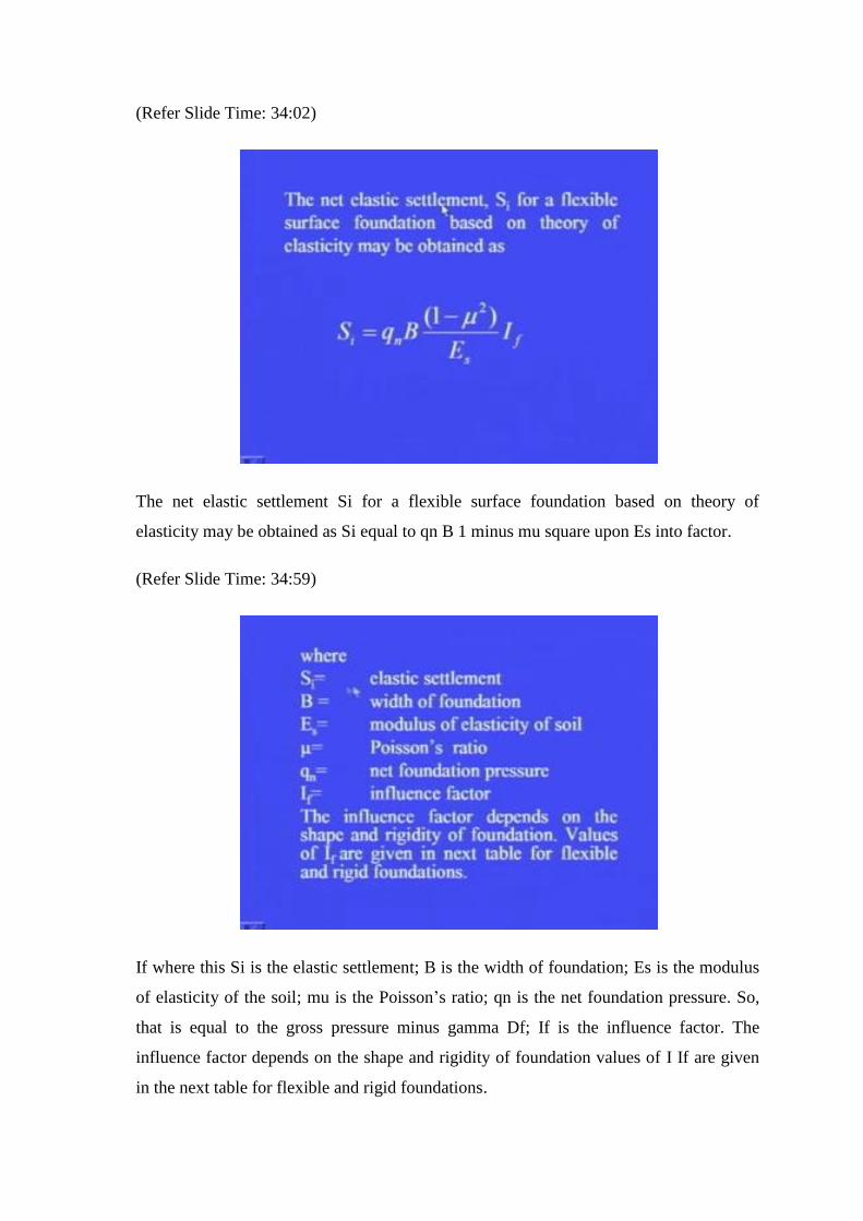
The net elastic settlement Si for a flexible surface foundation based on theory of

elasticity may be obtained as Si equal to qn B 1 minus mu square upon Es into factor.


If where this Si is the elastic settlement; B is the width of foundation; Es is the modulus

of elasticity of the soil; mu is the Poisson’s ratio; qn is the net foundation pressure. So,

that is equal to the gross pressure minus gamma Df; If is the influence factor. The

influence factor depends on the shape and rigidity of foundation values of I If are given

in the next table for flexible and rigid foundations.


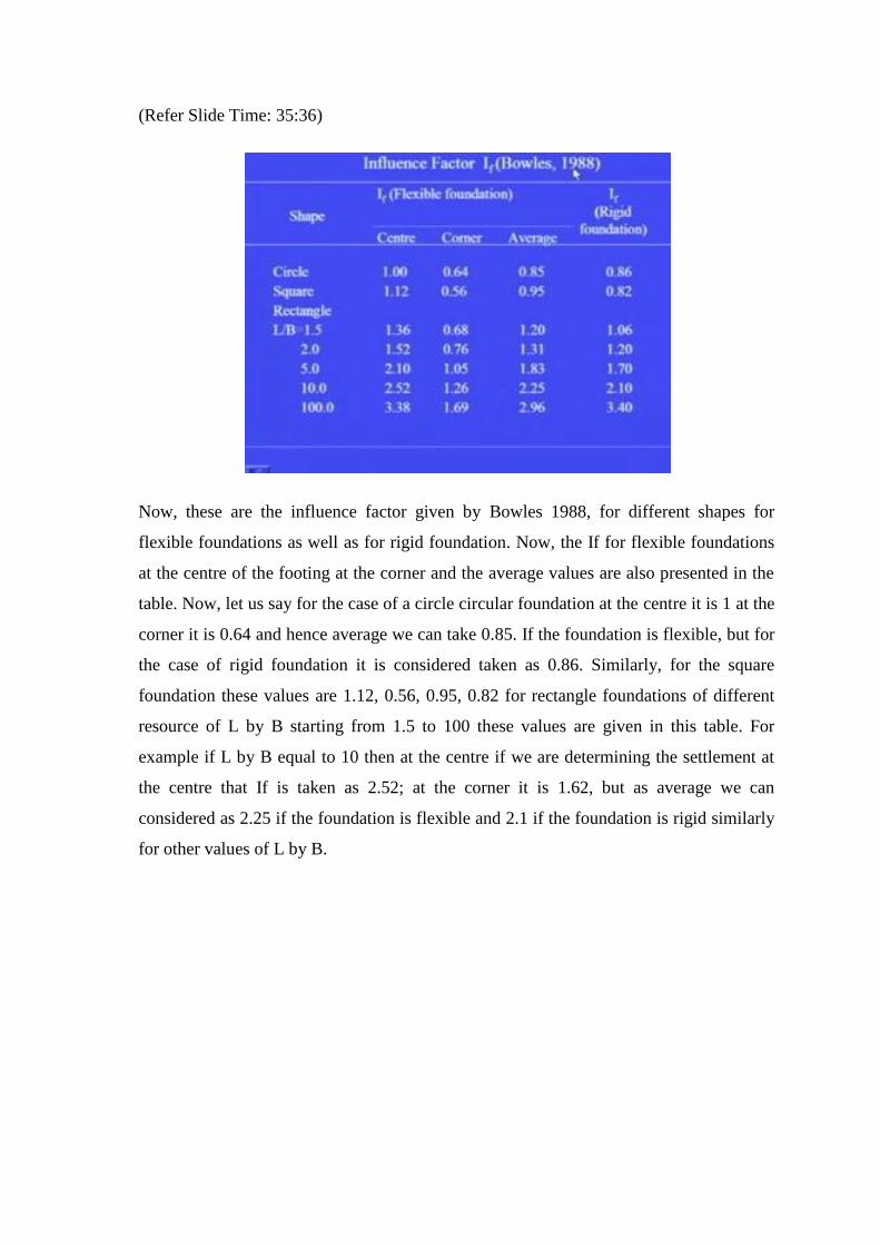
Now, these are the influence factor given by Bowles 1988, for different shapes for

flexible foundations as well as for rigid foundation. Now, the If for flexible foundations

at the centre of the footing at the corner and the average values are also presented in the

table. Now, let us say for the case of a circle circular foundation at the centre it is 1 at the

corner it is 0.64 and hence average we can take 0.85. If the foundation is flexible, but for

the case of rigid foundation it is considered taken as 0.86. Similarly, for the square

foundation these values are 1.12, 0.56, 0.95, 0.82 for rectangle foundations of different

resource of L by B starting from 1.5 to 100 these values are given in this table. For

example if L by B equal to 10 then at the centre if we are determining the settlement at

the centre that If is taken as 2.52; at the corner it is 1.62, but as average we can

considered as 2.25 if the foundation is flexible and 2.1 if the foundation is rigid similarly

for other values of L by B.


It can be seen that, the settlement of a rigid footing such as a beam and raft slab is

approximately equal to the mean settlement for a corresponding flexible foundation. For

example, steel tanks for storage of oil or earth fill are the examples of the flexible

foundations.


Typical range of values of Poisson’s ratio or dependent on the type of soil and it varies

from 0.1 to 0.5. Now, for the clay which is in saturated condition this value is taken as

0.4 to 0.5; 0.5 is the maximum for the undrained condition. For clay unsaturated it can be

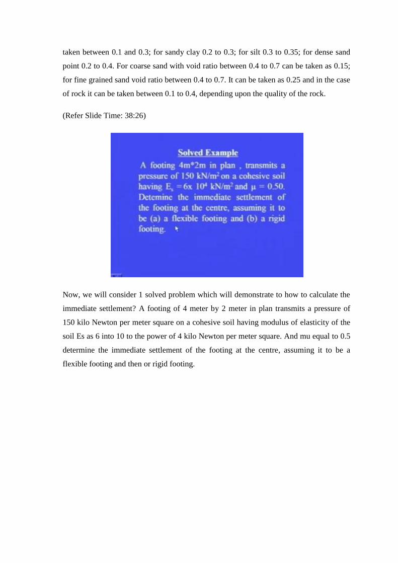
taken between 0.1 and 0.3; for sandy clay 0.2 to 0.3; for silt 0.3 to 0.35; for dense sand

point 0.2 to 0.4. For coarse sand with void ratio between 0.4 to 0.7 can be taken as 0.15;

for fine grained sand void ratio between 0.4 to 0.7. It can be taken as 0.25 and in the case

of rock it can be taken between 0.1 to 0.4, depending upon the quality of the rock.


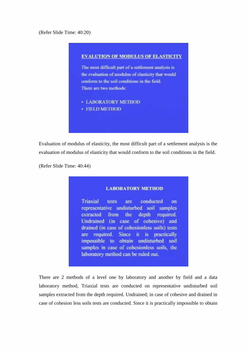
Now, we will consider 1 solved problem which will demonstrate to how to calculate the

immediate settlement? A footing of 4 meter by 2 meter in plan transmits a pressure of

150 kilo Newton per meter square on a cohesive soil having modulus of elasticity of the

soil Es as 6 into 10 to the power of 4 kilo Newton per meter square. And mu equal to 0.5

determine the immediate settlement of the footing at the centre, assuming it to be a

flexible footing and then or rigid footing.


1

So, we know that this Si is given by qn B 1 minus mu square upon Es into If. Now here

qn is given b is given mu is also given E is given only thing is we will have to select a

value of If. So, for L by B ratio of 2 from table which I have shown it earlier we can find

out that this If is 1 point for 1.52 for a flexible footing and 1.2 for a rigid footing. So,

when we substitute this value of If here we can find out immediate settlement for the

flexible as well as for the rigid footing. So, it comes out to be 5.7 millimeter for the

flexible footing and 4.5 millimeter for the rigid footing. If you use the rigidity factor of

0.5 as recommended by IS 8009 part 1 1976 then the S of the immediate settlement of

the footing, if we multiply with the flexible 0.8 into 5.7 it comes out to be 4.56. So, these

2 values you can see are comparable.


Evaluation of modulus of elasticity, the most difficult part of a settlement analysis is the

evaluation of modulus of elasticity that would conform to the soil conditions in the field.


There are 2 methods of a level one by laboratory and another by field and a data

laboratory method, Triaxial tests are conducted on representative undisturbed soil

samples extracted from the depth required. Undrained; in case of cohesive and drained in

case of cohesion less soils tests are conducted. Since it is practically impossible to obtain

undisturbed soil samples in case of cohesion less soils the laboratory method can be

ruled out.


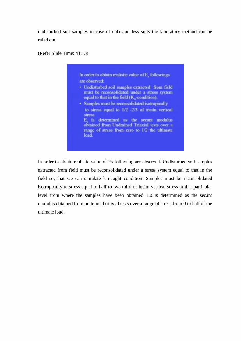
In order to obtain realistic value of Es following are observed. Undisturbed soil samples

extracted from field must be reconsolidated under a stress system equal to that in the

field so, that we can simulate k naught condition. Samples must be reconsolidated

isotropically to stress equal to half to two third of insitu vertical stress at that particular

level from where the samples have been obtained. Es is determined as the secant

modulus obtained from undrained triaxial tests over a range of stress from 0 to half of the

ultimate load.


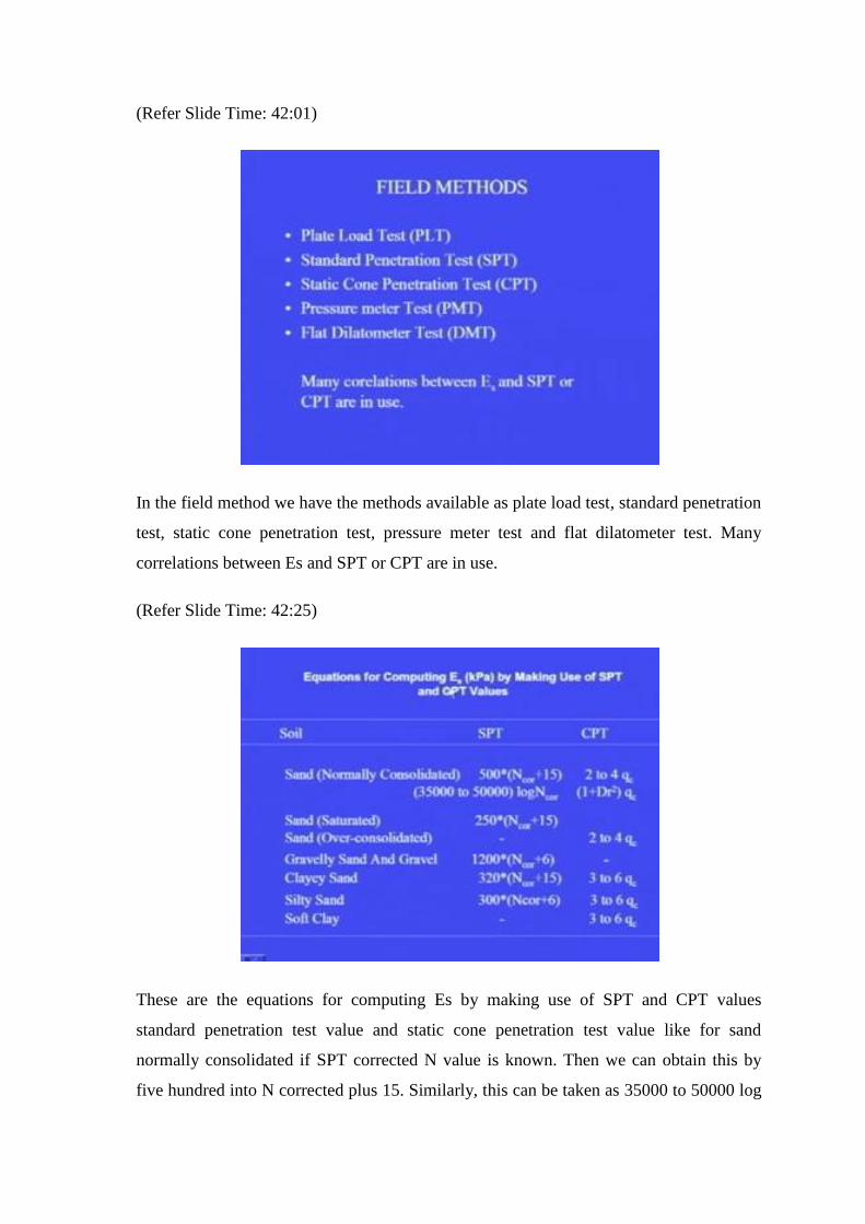
In the field method we have the methods available as plate load test, standard penetration

test, static cone penetration test, pressure meter test and flat dilatometer test. Many

correlations between Es and SPT or CPT are in use.


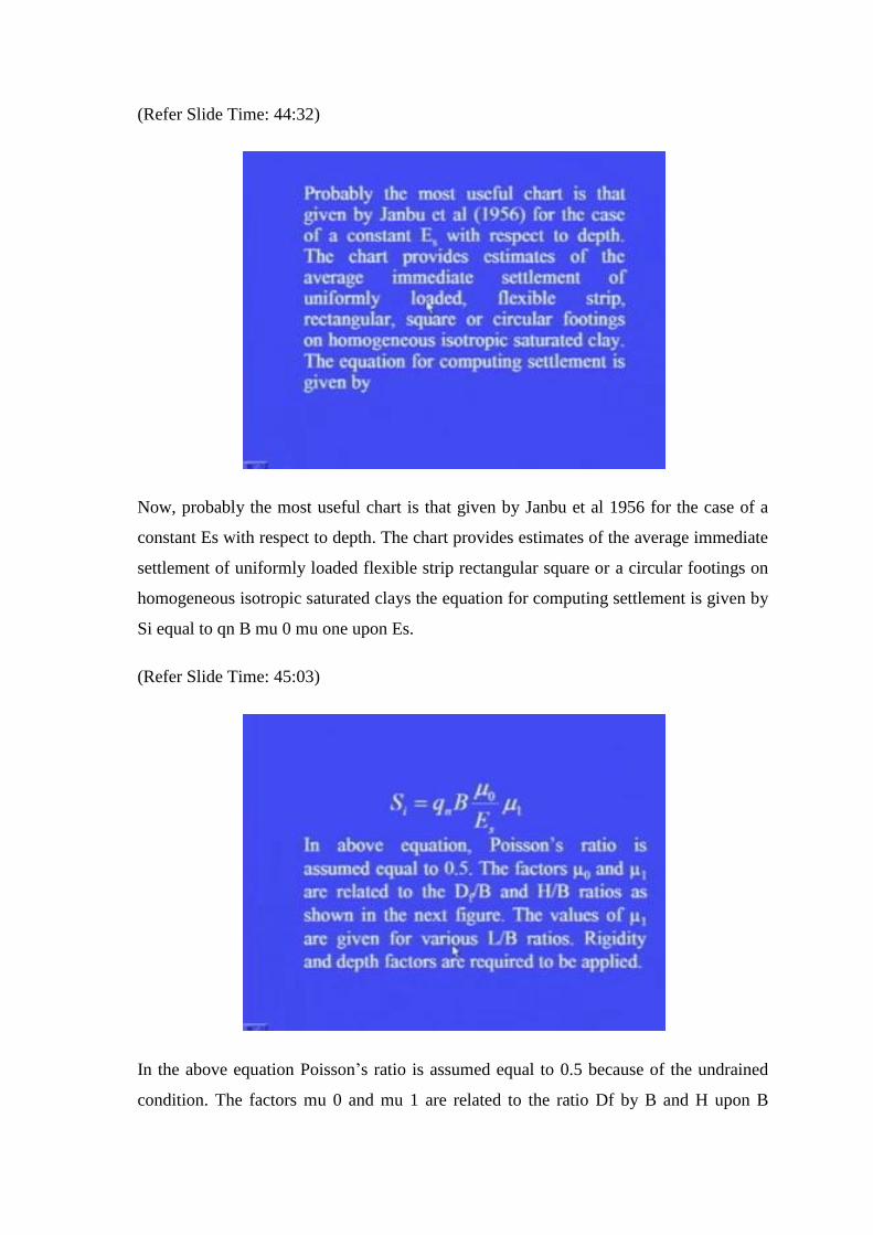
These are the equations for computing Es by making use of SPT and CPT values

standard penetration test value and static cone penetration test value like for sand

normally consolidated if SPT corrected N value is known. Then we can obtain this by

five hundred into N corrected plus 15. Similarly, this can be taken as 35000 to 50000 log

of N corrected for the case of normally consolidated sand if CPT values are available.

Then 2 to 4 times the qc or CPT value in the case of saturated sand it can be taken as 250

multiply by N corrected plus 15 in the case of over consolidated sand it can be taken as 2

to 4 of qc. If we have gravelly sand and gravels then we can use 1200 into N corrected

plus 6 if we have got clayey sand. Then 320 into N corrected plus 15 or 3 to 6 times of

qc silty sand 300 into N corrected plus 6 or 3 to 6 times of qc and if we have soft clay

then 3 to 6 times of qc.


So, by this method we can determine Es there is another method suggested by Janbu et al

for determining elastic settlement under undrained condition. Now, this is it can shows a

foundation which is a which is placed at a depth of Df and the load applied to the soil is

qn and width V is the width of the footing. And H is the depth of the soil layer below the

level of foundation the this strata below this is incompressible.


Now, probably the most useful chart is that given by Janbu et al 1956 for the case of a

constant Es with respect to depth. The chart provides estimates of the average immediate

settlement of uniformly loaded flexible strip rectangular square or a circular footings on

homogeneous isotropic saturated clays the equation for computing settlement is given by

Si equal to qn B mu 0 mu one upon Es.


In the above equation Poisson’s ratio is assumed equal to 0.5 because of the undrained

condition. The factors mu 0 and mu 1 are related to the ratio Df by B and H upon B

where H is the thickness of the soil layer below the foundation as shown in the next

figure. The values of mu one are given for various values of L upon B ratios rigidity and

depth factors are required to be applied.


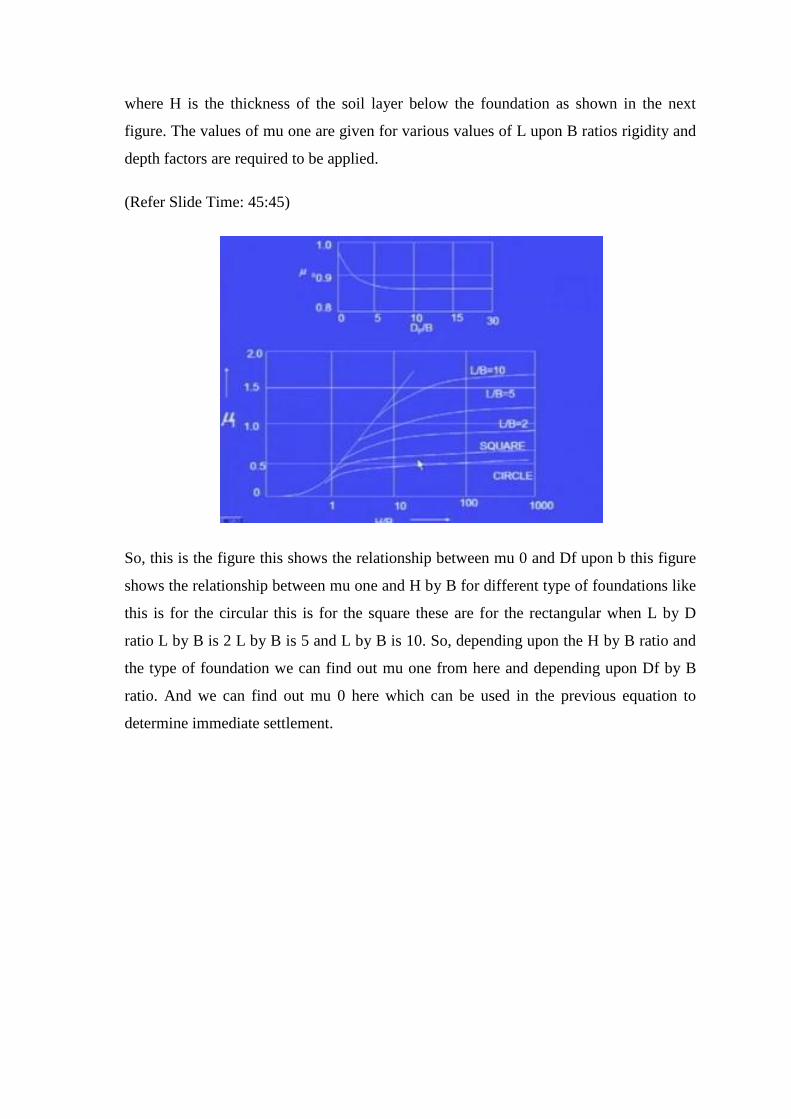
So, this is the figure this shows the relationship between mu 0 and Df upon b this figure

shows the relationship between mu one and H by B for different type of foundations like

this is for the circular this is for the square these are for the rectangular when L by D

ratio L by B is 2 L by B is 5 and L by B is 10. So, depending upon the H by B ratio and

the type of foundation we can find out mu one from here and depending upon Df by B

ratio. And we can find out mu 0 here which can be used in the previous equation to

determine immediate settlement.


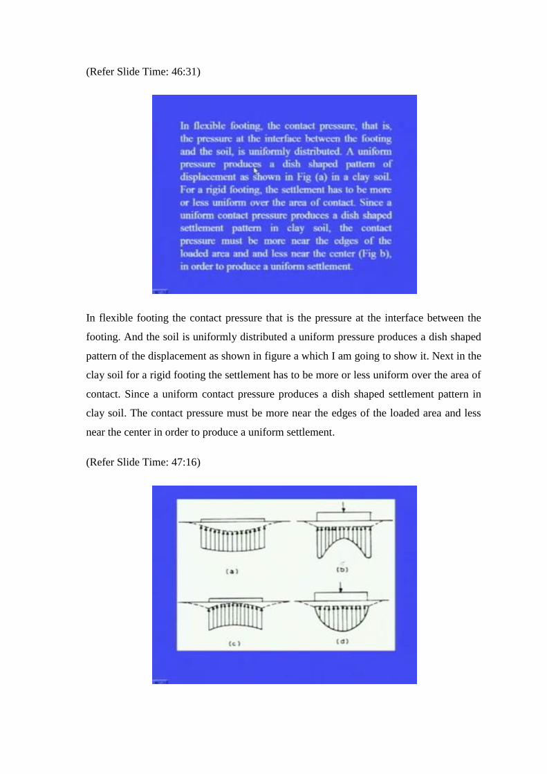
In flexible footing the contact pressure that is the pressure at the interface between the

footing. And the soil is uniformly distributed a uniform pressure produces a dish shaped

pattern of the displacement as shown in figure a which I am going to show it. Next in the

clay soil for a rigid footing the settlement has to be more or less uniform over the area of

contact. Since a uniform contact pressure produces a dish shaped settlement pattern in

clay soil. The contact pressure must be more near the edges of the loaded area and less

near the center in order to produce a uniform settlement.


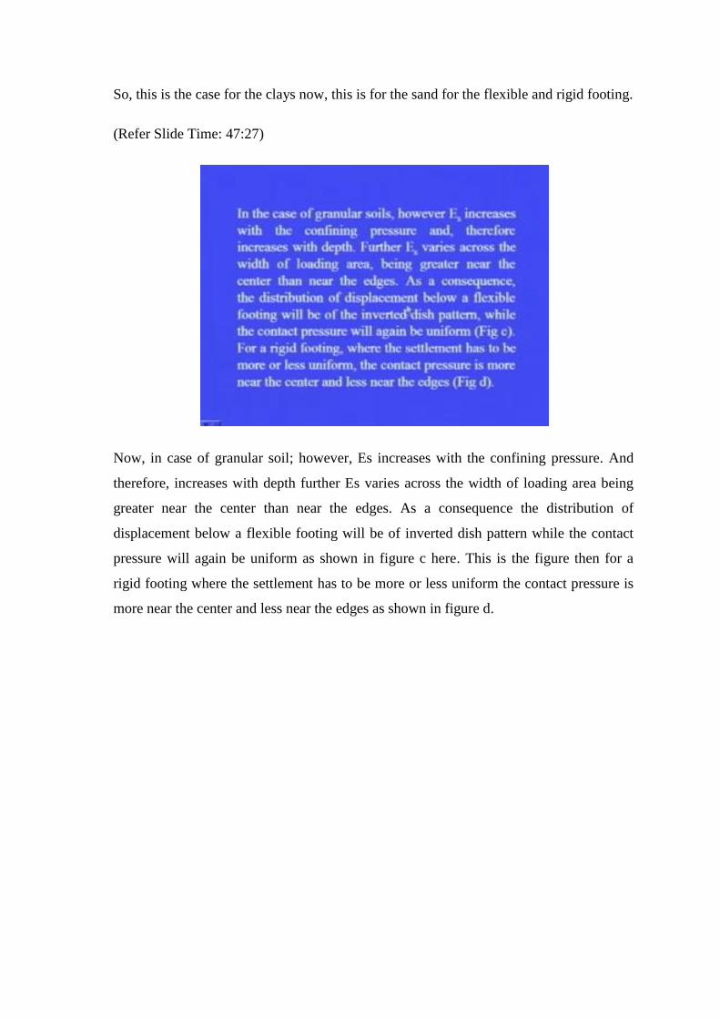
So, this is the case for the clays now, this is for the sand for the flexible and rigid footing.


Now, in case of granular soil; however, Es increases with the confining pressure. And

therefore, increases with depth further Es varies across the width of loading area being

greater near the center than near the edges. As a consequence the distribution of

displacement below a flexible footing will be of inverted dish pattern while the contact

pressure will again be uniform as shown in figure c here. This is the figure then for a

rigid footing where the settlement has to be more or less uniform the contact pressure is

more near the center and less near the edges as shown in figure d.


So, this is the figure for the rigid footing on granular soils Estimation of consolidation

settlement by using consolidation or Oedometer test data.


The consolidation settlement of saturated compressible stratum occurs due to expulsion

of pore water on account of gradual dissipation of excess pore water pressure induced by

an imposed total stress. In one dimensional compression the change in thickness delta h

per unit of original thickness H of the stratum is equal to the change in volume delta V

per unit of the original volume V.


The change in volume is a consequence of a decrease in the void ratio delta e as volume

of the soil solids remains unchanged. And the change in volume takes place due to

readjustment of the soil particles volume of solids will remain as it is.


So, using this concept we can determine the settlement the steps involved in the

consolidation settlement computations are as follows. First of all we determine the

subsoil profile. And in order to determine the subsoil profile collection of suitable soil

samples from different locations and depths determination of required soil parameters by

laboratory tests. Then calculation of pressures in the consolidating layers then the

calculation of consolidation settlement.


In order to determine this to find out this representative soil profile and soil properties

what is done an idealized soil profile which is representative of the average soil strata

((refer time: 50:10)) characteristics can be chosen. If a sufficient number of borings are

made at the site at properly selected locations from each boring information about the

nature of soil strata their thickness and position of natural water table will be available.

The soil samples taken from different locations and depths in different boreholes are then

tested in laboratory to obtain the index properties of different strata and to determine

consolidation parameters of the compressible stratum. One has to reconcile in the range

of variation in values and arrive at an average value applicable to the mid depth of the

consolidating stratum.


The second part is the analysis of pressure before and after loading. So, to determine the

pressure range under which the consolidation is caused one needs to find the effective

stress in the consolidating stratum before loading and increase in stress produced in the

stratum consequent to loading. Since both vary with the depth the average value of each

is used as a representative value for the soil layer in question. The mid depth values are

considered good enough if the thickness of the stratum is not very large in the case of a

thick consolidating layer. The practice is to divide the layer into number of layers whose

thickness does not exceed 1.5 meter. In the case of individual layers the mid depth values

of pressure or stress are used in the computations.


Once we have the knowledge of the soil profile location of water table and the index

properties of different strata. The initial effective stresses due to overburden at the mid

depth of individual layers can be very easily calculated for the simple static case of

hydrostatic pressure.


In the Terzaghi’s theory of 1 dimensional consolidation it is assumed that the application

of load produces an increase in pore water pressure in the entire consolidating layer

equal to the applied load and the consolidation is 1 dimensional. However, when the soil

is subjected to a load induced by a structure the distribution of initial excess hydrostatic

pressure with depth will not be uniform. But will assume the shape described by the

elastic theory of stress distribution.


Therefore in the computation of stresses transmitted to a buried clay layer by the loads of

the structure the Boussinesq or the Westergaard solution can be used to determine

increase in stress at the mid depth of the layer below individual columns. Or below the

center of raft foundation the approximate 2 vertical to 1 horizontal method of load

distribution may also be used. The Westergaard solutions is considered to be more close

to the conditions existing in sedimentary soils, and hence are preferred to the Boussinesq

solution.


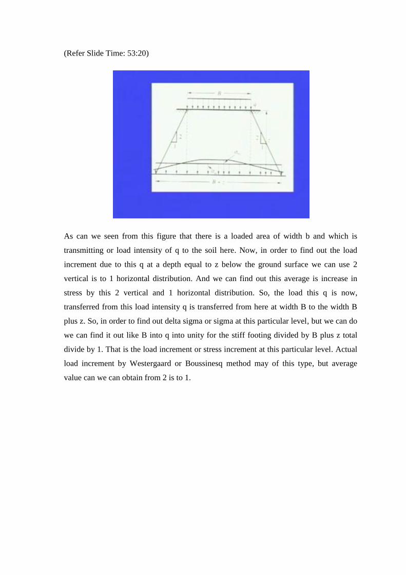
As can we seen from this figure that there is a loaded area of width b and which is

transmitting or load intensity of q to the soil here. Now, in order to find out the load

increment due to this q at a depth equal to z below the ground surface we can use 2

vertical is to 1 horizontal distribution. And we can find out this average is increase in

stress by this 2 vertical and 1 horizontal distribution. So, the load this q is now,

transferred from this load intensity q is transferred from here at width B to the width B

plus z. So, in order to find out delta sigma or sigma at this particular level, but we can do

we can find it out like B into q into unity for the stiff footing divided by B plus z total

divide by 1. That is the load increment or stress increment at this particular level. Actual

load increment by Westergaard or Boussinesq method may of this type, but average

value can we can obtain from 2 is to 1.


The consolidation test is performed in laboratory on the undisturbed specimen of clay

extracted from different locations and depths. The compressibility characteristics like

coefficient of compressibility av coefficient of volume compressibility Mv. And

compression index Cc may be determined by plotting curves between void ratio and

effective stress the pre consolidation pressure may also be determined. So, in this lecture

I have covered different field test by which we can determined ultimate bearing capacity

of soils. Then different aspects of settlement like immediate, elastic settlement or

consolidation settlement then the methods by which we can determine elastic settlement.

And I have started with the determination of consolidation settlement which I will

continue in the next lecture.

Thank you very much.

Documents

Foundation Engineering Prof. Dr N.K. Samadhiya …textofvideo.nptel.ac.in/105107120/lec4.pdf · have discussed the Terzaghi bearing capacity equation where half bearing capacity