Embed Size (px)
Citation preview
Journal of Mathematical Modelling and Algorithms 1: 193–214, 2002.© 2002 Kluwer Academic Publishers. Printed in the Netherlands.
193
Four Easy Ways to a Faster FFT �
LENORE R. MULLIN and SHARON G. SMALLComputer Science Department, University at Albany, SUNY, Albany, NY 12222, U.S.A. e-mail:{lenore, small}@cs.albany.edu
(Received: 25 September 2001; in final form: 21 May 2002)
Abstract. The Fast Fourier Transform (FFT) was named one of the Top Ten algorithms of the20th century, and continues to be a focus of current research. A problem with currently used FFTpackages is that they require large, finely tuned, machine specific libraries, produced by highly skilledsoftware developers. Therefore, these packages fail to perform well across a variety of architectures.Furthermore, many need to run repeated experiments in order to ‘re-program’ their code to its optimalperformance based on a given machine’s underlying hardware. Finally, it is difficult to know whichradix to use given a particular vector size and machine configuration. We propose the use of mono-lithic array analysis as a way to remove the constraints imposed on performance by a machine’sunderlying hardware, by pre-optimizing array access patterns. In doing this we arrive at a singleoptimized program. We have achieved up to a 99.6% increase in performance, and the ability torun vectors up to 8 388 608 elements larger, on our experimental platforms. Preliminary experimentsindicate different radices perform better relative to a machine’s underlying architecture.
Mathematics Subject Classifications (2000): 18C99, 68Q99, 55P55, 42A99, 18B99, 20J99.
Key words: performance analysis and evaluation, signal and image processing, FFT, array algebra,linear transformations, radix n, MOA, Psi calculus, shape polymorphism, shapes.
1. Introduction
Using our approach we have provided a new highly competitive version of the FFT,which performs well for all input vectors, without any knowledge of the underlyingarchitecture or the use of heuristics. Our method is based upon successive refine-ments, often involving transformations which use an associated array and indexcalculii, leading from the algebraic specification of the problem.
In general, our results indicate our approach can be beneficial to algorithmswhich have a common underlying algebraic structure and semantics. The FFT isan example of this type of algorithm and is the focus of our initial investigations.
We begin by discussing related work. We then describe the FFT, a Mathematicsof Arrays (MOA), and the Psi Calculus. We show how monolithic array analysis viaMOA creates the Three Easy Steps [33, 34], and how it can be used to extend thesteps to include a Fourth Step, the general radix FFT. Through experimentation on
� This work was partially supported by NSF CCR-9596184.
194 LENORE R. MULLIN AND SHARON G. SMALL
High Performance Computing (HPC) machines, we show how our approach out-performs current competitors. Finally, we discuss the direction of future research.
Several authors [12, 41, 42] have developed algebraic frameworks for a num-ber of these transforms and their discrete versions. Using their framework, manyvariant algorithms for the discrete versions of these transforms can be viewed ascomputing tensor products, using very similar data flow. Due to the importance ofthe FFT, numerous attempts have been made to optimize both performance andspace [10, 14, 16, 18].
There are various commercial and vendor specific libraries which include theFFT. The Numerical Analysis Group (NAG) and Visual Numerics (IMSL) provideand support finely tuned scientific libraries specific to various HPC platforms, e.g.SGI and IBM. The SGI and IBM libraries, SCSL and ESSL, are even more highlytuned, due to their knowledge of proprietary information specific to their respectivearchitectures. Another package, FFTW, has proven to be our leading competitor.Consequently, we have chosen to include all these packages in our comparativebenchmark studies.
Speed-ups due to parallelism have also been investigated [2, 9, 15, 17, 28].Language and compiler optimizations enable programs, in general, to obtain speed-ups. ZPL [5–7, 25], and C++ templates [44, 45], represent such features. TheBlitz++ system [46] provides generic C++ array objects, using expression tem-plates [45] to generate efficient code for array expressions. This system performsmany optimizations, including tiling and stride optimizations. C++ templates arealso used in POOMA, POOMA II [21, 23], and the Matrix Template Library (MTL)[26, 27]. MTL is a system that handles dense and sparse matrices, and uses templatemetaprograms to generate tiled algorithms for dense matrices.
Another approach for automatic generation and optimization of code to matchthe memory hierarchy and exploit pipelining is exemplified in ATLAS [47], whichoptimizes code for matrix multiply. In generating code, the ATLAS optimizer usestimings to determine blocking and loop unrolling factors. Another system thatgenerates matrix-multiply code matched to target architecture is PhiPAC [3]. HPF[20], MPI and OpenMP [1] use decomposition strategies to give the programmermechanisms to partition the problem based on their understanding of an algo-rithm’s memory access patterns. Skjellum [24, 39] uses polyalgorithms to achieveoptimizations across varying architectures.
The Fourier Transform is based on Gauss’ theory that any periodic wave may berepresented as a summation of a number of sine and cosine waves of different fre-quencies. The Fourier Transform computes the Fourier coefficients needed for thissummation. This transform takes samples of a signal over time and produces theFourier coefficients, allowing us to create a signal’s representation over a frequencyvariant. In its original formulation the Discrete Fourier Transform (DFT) has O(n2)
complexity. By analyzing the sparse matrix multiplication in the DFT and realizingthat only the diagonals of the blocks are used to decompose the matrices, a faster
FOUR EASY WAYS TO A FASTER FFT 195
O(n log n) formulation is possible, i.e. the FFT. The radix 2 Cooley-Tukey was thefirst fast formulation using this approach.
We use A Mathematics of Arrays (MOA) [29, 35–37], which relies on the PsiCalculus as a model to provide a mathematical framework for arrays, array index-ing, and array operations, to create our optimized code. The Psi Calculus includesrules, called Psi Reduction Rules, for transforming array expressions while pre-serving semantic equivalence. We used this array index calculus to control programtransformations in the development of our FFT algorithm.
2. Radix 2 FFT Implementation
STEP ONE: ALGORITHM DEFINITION
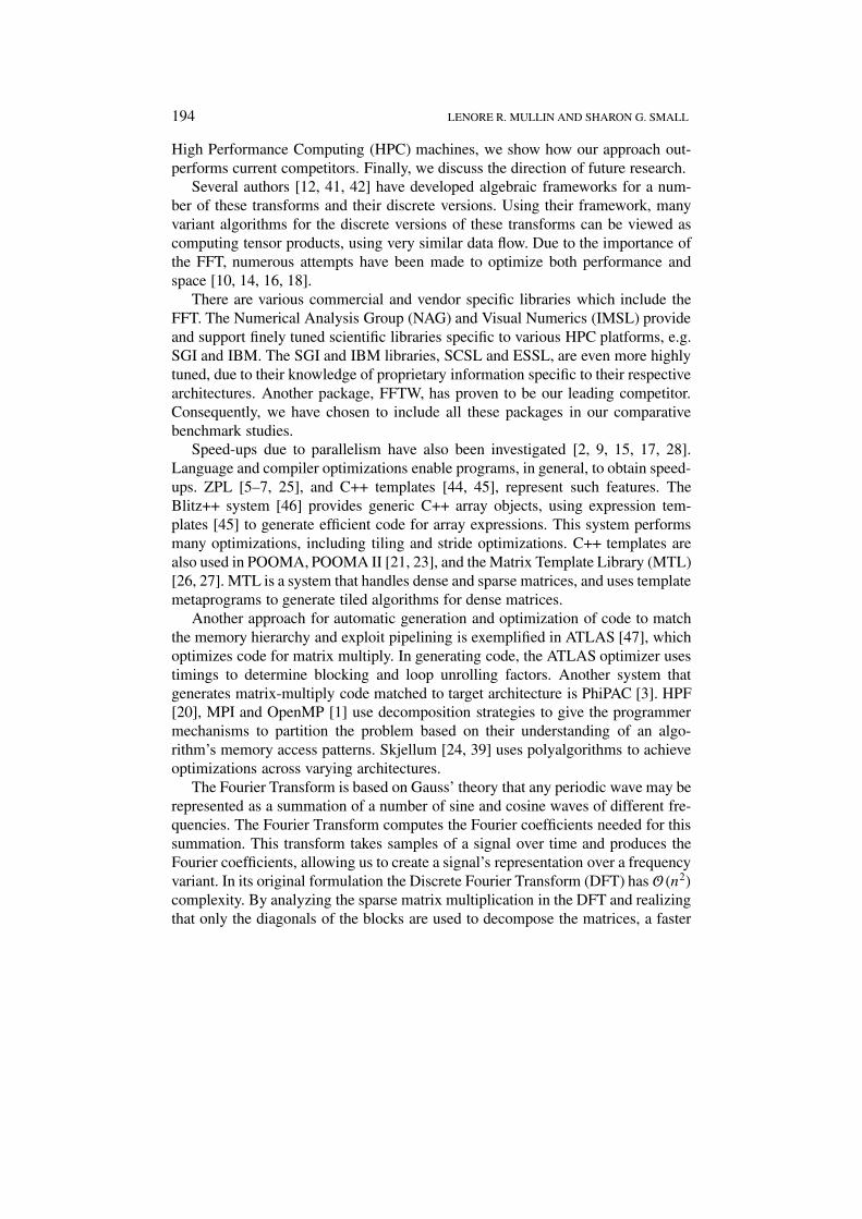
We began with Van Loan’s [43] high-level MATLAB� program for the radix 2 FFT,shown in Figure 1. This program denotes a single loop program, with high levelarray/vector operations and reshaping.
In Line 1, Pn is a permutation matrix that performs the bit-reversal permutationon the n elements of vector x. In Line 6, the n element array x is regarded as beingreshaped to be a L× r matrix consisting of r columns, each of which is a vector ofL elements. Line 6 can be viewed as treating each column of this matrix as a pair ofvectors, each with L/2 elements, and doing a butterfly computation that combinesthe two vectors in each pair to produce a vector with L elements.
The reshaping of the data matrix x in Line 6 is column-wise, so that each timeLine 6 is executed, each pair of adjacent columns of the preceding matrix areconcatenated to produce a column of the new matrix. The butterfly computation,corresponding to multiplication of the data matrix x by the weight matrix BL,
Input: x in Cn and n = 2t , where t � 0 is an integer.Output: The FFT of x.
x ← Pn x (1)for q = 1 to t (2)
begin (3)L← 2q (4)r ← n/L (5)xL×r ← BL xL×r (6)
end (7)
Here, Pn is a n × n permutation matrix, BL =[
IL∗ �L∗IL∗ −�L∗
],
L∗ = L/2, and �L∗ is a diagonal matrix with values 1, ωL, . . . , ωL∗−1L along
the diagonal, where ωL is the L’th root of unity.
Figure 1. High-level program for the radix 2 FFT.
� MATLAB is commonly used in the scientific community as a high-level prototyping language.
196 LENORE R. MULLIN AND SHARON G. SMALL
combines each pair of L/2 element column vectors from the old matrix into anew L element vector of values for each new column.
By direct inspection of Figure 1, the following three basic modules for the radix2 FFT can be identified.
(1) the computation of the bit-reversal permutation (Line 1),(2) the computation of the complex weights occurring in the matrices �L∗ . (Note:
Since L = 2q , the array BL is different for each iteration of the loop in Figure 1.Accordingly, the specification of IL∗ and �L∗ is parameterized by L (and henceimplicitly by q).)
(3) the butterfly computation that, using the weights, combines two vectors fromx, producing a vector with twice as many elements (Line 6).
A fourth basic module can be envisioned also:
(4) the generalization of the radix from two to n.
Generalizations of these three modules are appropriate components of arbitrarysize FFTs. More generally, analogues of these modules are appropriate for thewider class of FFT-like transforms [12].
STEP TWO: TUNING THE MATRIX AND DATA VECTOR
The weight constant matrix BL is a large two-dimensional sparse array, implyingthat most of the matrix multiply is not needed. Alternatively, this computation, canbe naturally specified by using constructors from the array calculus with a fewdense one-dimensional vectors as the basis. This yields a succinct description ofhow BL can be constructed via a composition of array operations. However, wenever actually materialize BL as a dense L× L matrix. Rather, the succinct repre-sentation is used to guide the generation of code for the FFT, and the generated codeonly has operations where multiplication by a nonzero element of BL is involved.
Note also, on the top-level, BL is constructed by the appropriate concatenationof four submatrices. Each of these four submatrices is a diagonal matrix. For eachof these diagonal matrices, the values along the diagonal are successive powers ofa given scalar. However, only the construction of two of these matrices, namelyIL∗ and �L∗ , need be independently specified. Matrix IL∗ occurs twice in the de-composition of BL. Matrix −�L∗ can be obtained from matrix �L∗ by applyingelement-wise unary minus.
There is an MOA constructor that produces a vector, which we denote as weight,whose elements are consecutive multiples or powers of a given scalar value.
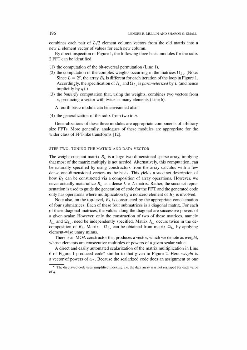
A direct and easily automated scalarization of the matrix multiplication in Line6 of Figure 1 produced code� similar to that given in Figure 2. Here weight isa vector of powers of ωL. Because the scalarized code does an assignment to one
� The displayed code uses simplified indexing, i.e. the data array was not reshaped for each valueof q.
FOUR EASY WAYS TO A FASTER FFT 197
do col = 0,r-1do row = 0,L-1
if (row < L/2 ) thenxx(row,col) = x(row,col) + weight(row)*x(row+L/2,col)
elsexx(row,col) = x(row-L/2,col) - weight(row-L/2)*x(row,col)
end ifend do
end do
Figure 2. Direct scalarization of the matrix multiplication.
do col = 0,r-1do row = 0,L-1
if (row < L/2 ) thenxx(L*col+row) = x(L*col+row) + weight(row)*x(L*col+row+L/2)
elsexx(L*col+row) = x(L*col+row-L/2) - weight(row-L/2)*x(L*col+row)
end ifend do
end do
Figure 3. Scalarized code with data stored in a vector.
element at a time, the generated code computes the result of the array multiplicationusing a temporary array xx, as shown below, and then copies xx into x.
The sparseness of matrix BL is reflected in the assignments to xx(row,col), asfollows. The right-hand side of these assignment statements is the sum of only thetwo terms that correspond to the two nonzero elements of the row of BL involvedin the computation of the left-hand side. The multiplication by the constant 1 fromthe matrix IL∗ is done implicitly in the generated code.
The data array x in Figure 1 is a two-dimensional array, that is reshaped duringeach iteration. Computationally, however, it is more efficient to store the data valuesin x as a one dimensional vector, and to avoid reshaping completely. MOA’s indexcalculus easily automates such transformations as the mapping of indices of anelement of the two-dimensional array into the index of the corresponding elementof the vector.
The L × r matrix xL×r is stored as an n-element vector, which we denote asx. This is done in column-major order, reflecting the column-wise reshaping oc-curring in Figure 1. Thus, element xL×r (row, col) of xL×r corresponds to elementx(L∗col+row) of x. Consequently, when L changes, and matrix xL×r is reshaped,no movement of data elements of vector x actually occurs.
Generating the same scalarized code as above, but with each access to an ele-ment of the two-dimensional matrix xL×r replaced by an access to the correspond-ing element of the vector x, produces the code shown in Figure 3.
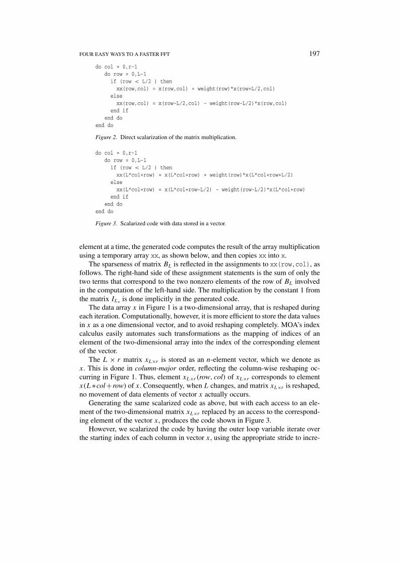
However, we scalarized the code by having the outer loop variable iterate overthe starting index of each column in vector x, using the appropriate stride to incre-
198 LENORE R. MULLIN AND SHARON G. SMALL
do col′ = 0,n-1,Ldo row = 0,L-1
if (row < L/2 ) thenxx(col′+row) = x(col′+row) + weight(row)*x(col′+row+L/2)
elsexx(col′+row) = x(col′+row-L/2) - weight(row-L/2)*x(col′+row)
end ifend do
end do
Figure 4. Striding through the data vector.
do col = 0,r-1do row = 0,L/2-1
do group = 0,1if ( group == 0 ) thenxx(row,group,col) =
x(row,group,col) + weight(row)*x(row,group+1,col)elsexx(row,group,col) =
x(row,group-1,col) - weight(row)*x(row,group,col)end if
end doend do
end do
Figure 5. Retiled loop.
ment this loop variable. Thus, instead of using a loop variable col, which rangesfrom 0 to r − 1 with a stride of 1, we use a variable, say col′, such that col′ =L ∗ col, and which consequently has a stride of L. By doing this, we eliminate themultiplication L ∗ col that occurs each time an element of the arrays xx or x isaccessed.
This form of scalarization produced the code shown in Figure 4.
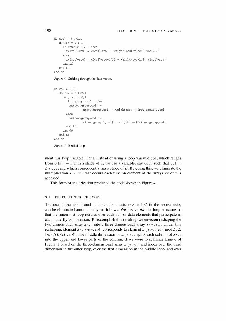
STEP THREE: TUNING THE CODE
The use of the conditional statement that tests row < L/2 in the above code,can be eliminated automatically, as follows. We first re-tile the loop structure sothat the innermost loop iterates over each pair of data elements that participate ineach butterfly combination. To accomplish this re-tiling, we envision reshaping thetwo-dimensional array xL×r into a three-dimensional array xL/2×2×r . Under thisreshaping, element xL×r (row, col) corresponds to element xL/2×2×r (row mod L/2,
�row/(L/2), col). The middle dimension of xL/2×2×r splits each column of xL×r
into the upper and lower parts of the column. If we were to scalarize Line 6 ofFigure 1 based on the three-dimensional array xL/2×2×r , and index over the thirddimension in the outer loop, over the first dimension in the middle loop, and over
FOUR EASY WAYS TO A FASTER FFT 199
do col = 0,r-1do row = 0,L/2-1
xx(row,0,col) =x(row,0,col) + weight(row)*x(row,1,col)
xx(row,1,col) =x(row,0,col) - weight(row)*x(row,1,col)
end doend do
Figure 6. Unrolled inner loop.
do col′ = 0,n-1,Ldo row = 0,L/2-1
xx(col′+row) = x(col′+row) +weight(row)*x(col′+row+L/2)
xx(col′+row+L/2) = x(col′+row) -weight(row)*x(col′+row+L/2)
end doend do
Figure 7. Unrolled loop with data stored as a vector.
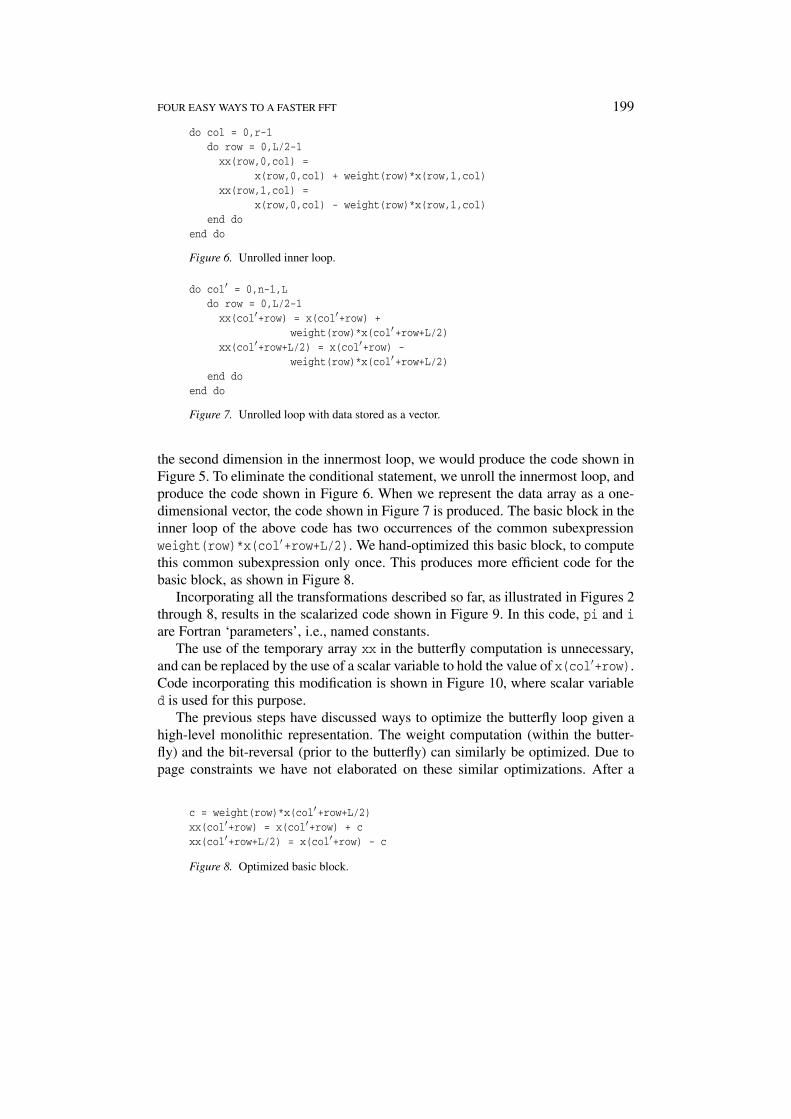
the second dimension in the innermost loop, we would produce the code shown inFigure 5. To eliminate the conditional statement, we unroll the innermost loop, andproduce the code shown in Figure 6. When we represent the data array as a one-dimensional vector, the code shown in Figure 7 is produced. The basic block in theinner loop of the above code has two occurrences of the common subexpressionweight(row)*x(col′+row+L/2). We hand-optimized this basic block, to computethis common subexpression only once. This produces more efficient code for thebasic block, as shown in Figure 8.
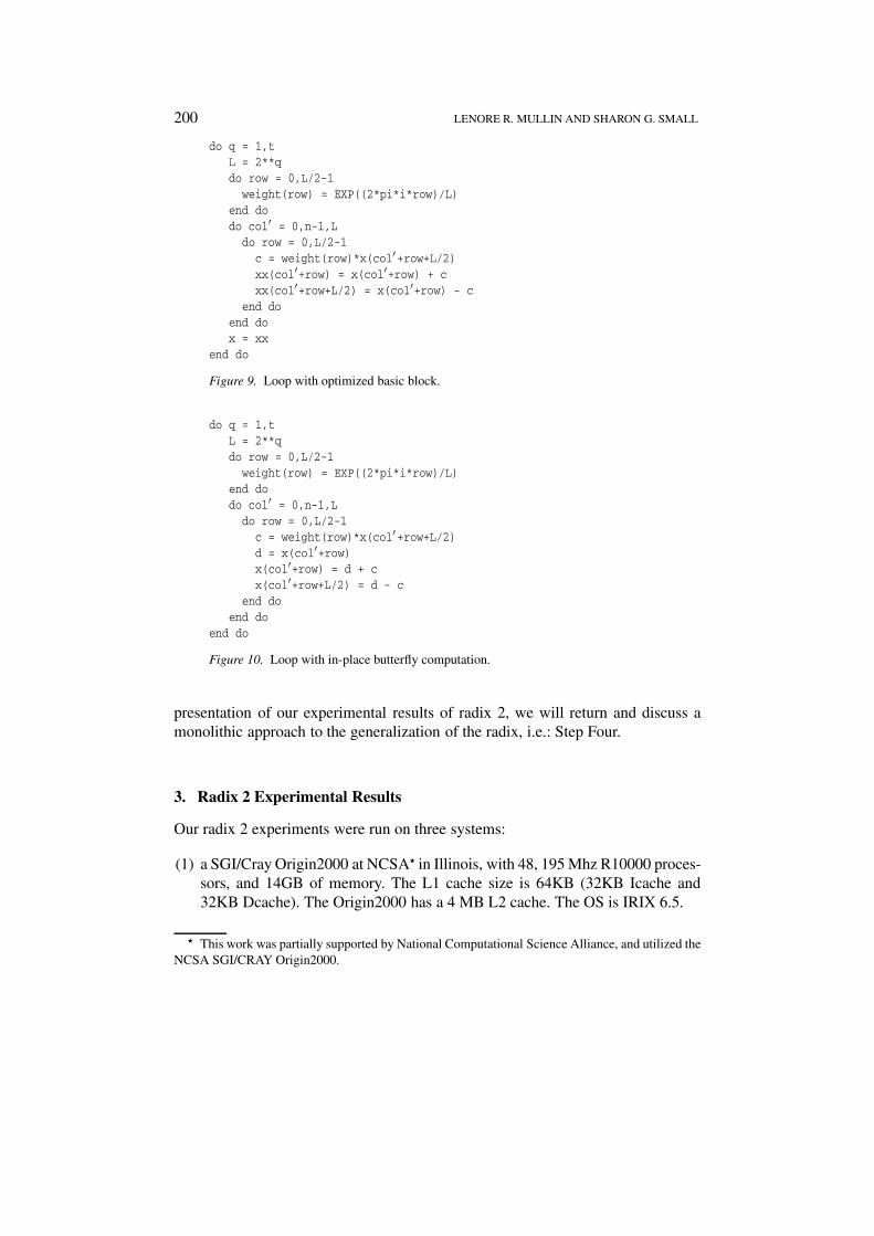
Incorporating all the transformations described so far, as illustrated in Figures 2through 8, results in the scalarized code shown in Figure 9. In this code, pi and iare Fortran ‘parameters’, i.e., named constants.
The use of the temporary array xx in the butterfly computation is unnecessary,and can be replaced by the use of a scalar variable to hold the value of x(col′+row).Code incorporating this modification is shown in Figure 10, where scalar variabled is used for this purpose.
The previous steps have discussed ways to optimize the butterfly loop given ahigh-level monolithic representation. The weight computation (within the butter-fly) and the bit-reversal (prior to the butterfly) can similarly be optimized. Due topage constraints we have not elaborated on these similar optimizations. After a
c = weight(row)*x(col′+row+L/2)xx(col′+row) = x(col′+row) + cxx(col′+row+L/2) = x(col′+row) - c
Figure 8. Optimized basic block.
200 LENORE R. MULLIN AND SHARON G. SMALL
do q = 1,tL = 2**qdo row = 0,L/2-1
weight(row) = EXP((2*pi*i*row)/L)end dodo col′ = 0,n-1,L
do row = 0,L/2-1c = weight(row)*x(col′+row+L/2)xx(col′+row) = x(col′+row) + cxx(col′+row+L/2) = x(col′+row) - c
end doend dox = xx
end do
Figure 9. Loop with optimized basic block.
do q = 1,tL = 2**qdo row = 0,L/2-1
weight(row) = EXP((2*pi*i*row)/L)end dodo col′ = 0,n-1,L
do row = 0,L/2-1c = weight(row)*x(col′+row+L/2)d = x(col′+row)x(col′+row) = d + cx(col′+row+L/2) = d - c
end doend do
end do
Figure 10. Loop with in-place butterfly computation.
presentation of our experimental results of radix 2, we will return and discuss amonolithic approach to the generalization of the radix, i.e.: Step Four.
3. Radix 2 Experimental Results
Our radix 2 experiments were run on three systems:
(1) a SGI/Cray Origin2000 at NCSA� in Illinois, with 48, 195 Mhz R10000 proces-sors, and 14GB of memory. The L1 cache size is 64KB (32KB Icache and32KB Dcache). The Origin2000 has a 4 MB L2 cache. The OS is IRIX 6.5.
� This work was partially supported by National Computational Science Alliance, and utilized theNCSA SGI/CRAY Origin2000.
FOUR EASY WAYS TO A FASTER FFT 201
(2) an IBM SP-2 at the MAUI High Performance Computing Center�, with 32,P2SC 160 Mhz processors, and 1GB of memory. The L1 cache size is 160KB(32KB Icache and 128KB Dcache), there is no L2 cache. The OS is AIX 4.3.
(3) a SUN SPARCserver1000E, with 2, 60 Mhz processors, and 128MB of mem-ory. Its L1 cache size is 36KB (20KB Icache and 16KB Dcache) and it isone-way set associative. The OS is Solaris 2.7.
We tested against the FFTW on all three machines and against the math librariessupported on the IBM SP-2 and the Origin 2000 machines; on the Origin 2000:IMSL Fortran Numerical Libraries version 3.01, NAG version Mark 19, and SGI’sSCSL library, and on the SP-2: IBM’s ESSL library.
Experiments on the Origin 2000 were run using bsub, SGI’s batch processingenvironment. Similarly, on the SP-2 experiments were run using loadleveler. Inboth cases we used dedicated networks and processors. The SPARCserver 1000Ewas a machine dedicated to runing our experiments. Experiments were repeateda minimum of three times and averaged for each vector size (23 to 224). Vendorcompilers were used with the -O3 and -Inline flags, for improved optimizations.We used Perl scripts to automatically compile, run, time all experiments, and toplot our results for various problem sizes.
We believe thatthe only consistent and reliable measure of performance is the execution timeof real programs, and that all proposed alternatives to time as the metric or toreal programs as the items measured have eventually led to misleading claimsor even mistakes in computer design. [19]Therefore, we time the execution of the entire executable, which includes the
creation of the FFTW plan. Although FFTW claims a plan can be reused, the planis a data structure and not easily saved. Therefore, they have developed a utilitycalled wisdom, which still requires partial plan regeneration.
FFTW implements a method for saving plans to disk and restoring them. Themechanism is called wisdom. There are pitfalls to using wisdom, in that it cannegate FFTW’s ability to adapt to changing hardware and other conditions.Actually, the optimal plan may change even between runs of the same binaryon identical hardware, due to differences in the virtual memory environment.It is therefore wise to recreate wisdom every time an application is recompiled.[13]
This is further confirmed by the fact that when we ran FFTW’s test programon our dedicated machines. We found surprising differences in time for the samevector size. Our dedicated machines ran a default OS, e.g. no special quantum,queue settings, or kernel tuning. Due to this, a plan should be as current as possible.
IMSL, NAG, SCSL, and ESSL required no plan generation. The entire execu-tion of code created to use each library’s FFT was timed.
� We would like to thank the Maui High Performance Computing Center for access to their IBMSP-2.
202 LENORE R. MULLIN AND SHARON G. SMALL
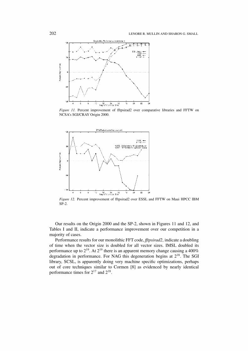
Figure 11. Percent improvement of fftpsirad2 over comparative libraries and FFTW onNCSA’s SGI/CRAY Origin 2000.
Figure 12. Percent improvement of fftpsirad2 over ESSL and FFTW on Maui HPCC IBMSP-2.
Our results on the Origin 2000 and the SP-2, shown in Figures 11 and 12, andTables I and II, indicate a performance improvement over our competition in amajority of cases.
Performance results for our monolithic FFT code, fftpsirad2, indicate a doublingof time when the vector size is doubled for all vector sizes. IMSL doubled itsperformance up to 219. At 219 there is an apparent memory change causing a 400%degradation in performance. For NAG this degeneration begins at 218. The SGIlibrary, SCSL, is apparently doing very machine specific optimizations, perhapsout of core techniques similar to Cormen [8] as evidenced by nearly identicalperformance times for 217 and 218.
FOUR EASY WAYS TO A FASTER FFT 203
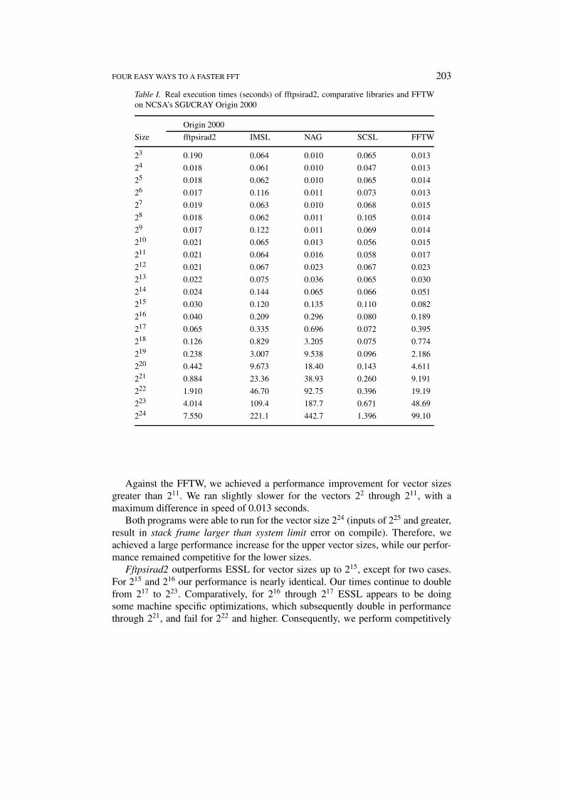
Table I. Real execution times (seconds) of fftpsirad2, comparative libraries and FFTWon NCSA’s SGI/CRAY Origin 2000
Origin 2000
Size fftpsirad2 IMSL NAG SCSL FFTW
23 0.190 0.064 0.010 0.065 0.013
24 0.018 0.061 0.010 0.047 0.013
25 0.018 0.062 0.010 0.065 0.014
26 0.017 0.116 0.011 0.073 0.013
27 0.019 0.063 0.010 0.068 0.015
28 0.018 0.062 0.011 0.105 0.014
29 0.017 0.122 0.011 0.069 0.014
210 0.021 0.065 0.013 0.056 0.015
211 0.021 0.064 0.016 0.058 0.017
212 0.021 0.067 0.023 0.067 0.023
213 0.022 0.075 0.036 0.065 0.030
214 0.024 0.144 0.065 0.066 0.051
215 0.030 0.120 0.135 0.110 0.082
216 0.040 0.209 0.296 0.080 0.189
217 0.065 0.335 0.696 0.072 0.395
218 0.126 0.829 3.205 0.075 0.774
219 0.238 3.007 9.538 0.096 2.186
220 0.442 9.673 18.40 0.143 4.611
221 0.884 23.36 38.93 0.260 9.191
222 1.910 46.70 92.75 0.396 19.19
223 4.014 109.4 187.7 0.671 48.69
224 7.550 221.1 442.7 1.396 99.10
Against the FFTW, we achieved a performance improvement for vector sizesgreater than 211. We ran slightly slower for the vectors 22 through 211, with amaximum difference in speed of 0.013 seconds.
Both programs were able to run for the vector size 224 (inputs of 225 and greater,result in stack frame larger than system limit error on compile). Therefore, weachieved a large performance increase for the upper vector sizes, while our perfor-mance remained competitive for the lower sizes.
Fftpsirad2 outperforms ESSL for vector sizes up to 215, except for two cases.For 215 and 216 our performance is nearly identical. Our times continue to doublefrom 217 to 223. Comparatively, for 216 through 217 ESSL appears to be doingsome machine specific optimizations, which subsequently double in performancethrough 221, and fail for 222 and higher. Consequently, we perform competitively
204 LENORE R. MULLIN AND SHARON G. SMALL
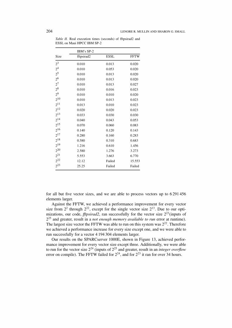
Table II. Real execution times (seconds) of fftpsirad2 andESSL on Maui HPCC IBM SP-2
IBM’s SP-2
Size fftpsirad2 ESSL FFTW
23 0.010 0.013 0.020
24 0.010 0.053 0.020
25 0.010 0.013 0.020
26 0.010 0.013 0.020
27 0.010 0.013 0.027
28 0.010 0.016 0.023
29 0.010 0.010 0.020
210 0.010 0.013 0.023
211 0.013 0.010 0.023
212 0.020 0.020 0.023
213 0.033 0.030 0.030
214 0.040 0.043 0.053
215 0.070 0.060 0.083
216 0.140 0.120 0.143
217 0.280 0.160 0.283
218 0.580 0.310 0.683
219 1.216 0.610 1.456
220 2.580 1.276 3.273
221 5.553 3.663 6.770
222 12.12 Failed 15.553
223 25.25 Failed Failed
for all but five vector sizes, and we are able to process vectors up to 6 291 456elements larger.
Against the FFTW, we achieved a performance improvement for every vectorsize from 22 through 222, except for the single vector size 213. Due to our opti-mizations, our code, fftpsirad2, ran successfully for the vector size 223(inputs of225 and greater, result in a not enough memory available to run error at runtime).The largest size vector the FFTW was able to run on this system was 222. Thereforewe achieved a performance increase for every size except one, and we were able torun successfully for a vector 4 194 304 elements larger.
Our results on the SPARCserver 1000E, shown in Figure 13, achieved perfor-mance improvement for every vector size except three. Additionally, we were ableto run for the vector size 224 (inputs of 225 and greater, result in an integer overflowerror on compile). The FFTW failed for 224, and for 223 it ran for over 34 hours.
FOUR EASY WAYS TO A FASTER FFT 205
Figure 13. Percent improvement of fftpsirad2 over FFTW on SPARCserver 1000E.
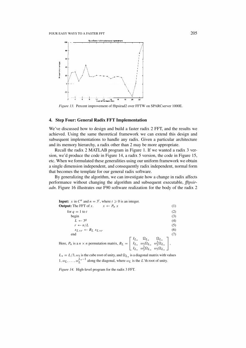
4. Step Four: General Radix FFT Implementation
We’ve discussed how to design and build a faster radix 2 FFT, and the results weachieved. Using the same theoretical framework we can extend this design andsubsequent implementations to handle any radix. Given a particular architectureand its memory hierarchy, a radix other than 2 may be more appropriate.
Recall the radix 2 MATLAB program in Figure 1. If we wanted a radix 3 ver-sion, we’d produce the code in Figure 14, a radix 5 version, the code in Figure 15,etc. When we formulated these generalities using our uniform framework we obtaina single dimension independent, and consequently radix independent, normal formthat becomes the template for our general radix software.
By generalizing the algorithm, we can investigate how a change in radix affectsperformance without changing the algorithm and subsequent executable, fftpsir-adn. Figure 16 illustrates our F90 software realization for the body of the radix 2
Input: x in Cn and n = 3t , where t � 0 is an integer.Output: The FFT of x. x ← Pn x (1)
for q = 1 to t (2)begin (3)
L← 3q (4)r ← n/L (5)xL×r ← BL xL×r (6)
end (7)
Here, Pn is a n× n permutation matrix, BL = IL∗ �L∗ �L∗
IL∗ ω3�L∗ ω23�L∗
IL∗ ω23�L∗ ω3�L∗
,
L∗ = L/3, ω3 is the cube root of unity, and �L∗ is a diagonal matrix with values
1, ωL, . . . , ωL∗−1L
along the diagonal, where ωL is the L’th root of unity.
Figure 14. High-level program for the radix 3 FFT.
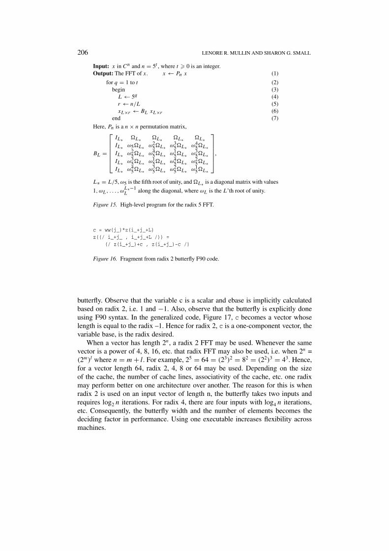
206 LENORE R. MULLIN AND SHARON G. SMALL
Input: x in Cn and n = 5t , where t � 0 is an integer.Output: The FFT of x. x ← Pn x (1)
for q = 1 to t (2)begin (3)
L← 5q (4)r ← n/L (5)xL×r ← BL xL×r (6)
end (7)
Here, Pn is a n× n permutation matrix,
BL =
IL∗ �L∗ �L∗ �L∗ �L∗IL∗ ω5�L∗ ω2
5�L∗ ω35�L∗ ω4
5�L∗IL∗ ω2
5�L∗ ω45�L∗ ω1
5�L∗ ω35�L∗
IL∗ ω35�L∗ ω1
5�L∗ ω45�L∗ ω2
5�L∗IL∗ ω4
5�L∗ ω35�L∗ ω2
5�L∗ ω15�L∗
,
L∗ = L/5, ω5 is the fifth root of unity, and �L∗ is a diagonal matrix with values
1, ωL, . . . , ωL∗−1L along the diagonal, where ωL is the L’th root of unity.
Figure 15. High-level program for the radix 5 FFT.
c = ww(j_)*z(i_+j_+L)z((/ i_+j_ , i_+j_+L /)) =
(/ z(i_+j_)+c , z(i_+j_)-c /)
Figure 16. Fragment from radix 2 butterfly F90 code.
butterfly. Observe that the variable c is a scalar and ebase is implicitly calculatedbased on radix 2, i.e. 1 and −1. Also, observe that the butterfly is explicitly doneusing F90 syntax. In the generalized code, Figure 17, c becomes a vector whoselength is equal to the radix –1. Hence for radix 2, c is a one-component vector, thevariable base, is the radix desired.
When a vector has length 2n, a radix 2 FFT may be used. Whenever the samevector is a power of 4, 8, 16, etc. that radix FFT may also be used, i.e. when 2n =(2m)l where n = m+ l. For example, 25 = 64 = (23)2 = 82 = (22)3 = 43. Hence,for a vector length 64, radix 2, 4, 8 or 64 may be used. Depending on the sizeof the cache, the number of cache lines, associativity of the cache, etc. one radixmay perform better on one architecture over another. The reason for this is whenradix 2 is used on an input vector of length n, the butterfly takes two inputs andrequires log2 n iterations. For radix 4, there are four inputs with log4 n iterations,etc. Consequently, the butterfly width and the number of elements becomes thedeciding factor in performance. Using one executable increases flexibility acrossmachines.
FOUR EASY WAYS TO A FASTER FFT 207
c(start) = z(i_+j_)ebase(start) =do k_=start+1,base-1
c(k_) = ww(j_*k_)*z(i_+j_+(k_*L))z(i_+j_) = z(i_+j_)+c(k_)ebase(k_)=EXP((-2*pi*i)/base)**k_
end do
do k_=start+1,base-1temp = c(start)do l_=start+1,base-1
temp = temp+c(l_)*ebase(modulo((k_*l_),base))
end doz(i_+j_+(k_*L))=temp
end do
Figure 17. Fragment from Radix n F90 code.
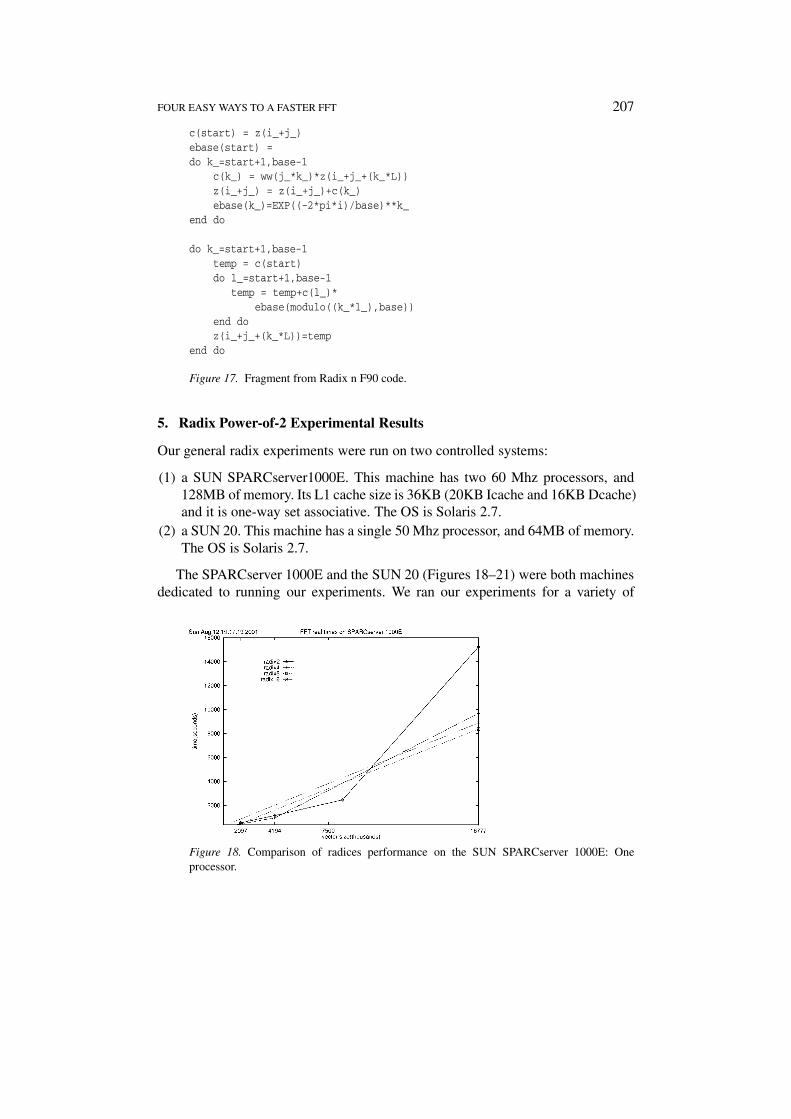
5. Radix Power-of-2 Experimental Results
Our general radix experiments were run on two controlled systems:
(1) a SUN SPARCserver1000E. This machine has two 60 Mhz processors, and128MB of memory. Its L1 cache size is 36KB (20KB Icache and 16KB Dcache)and it is one-way set associative. The OS is Solaris 2.7.
(2) a SUN 20. This machine has a single 50 Mhz processor, and 64MB of memory.The OS is Solaris 2.7.
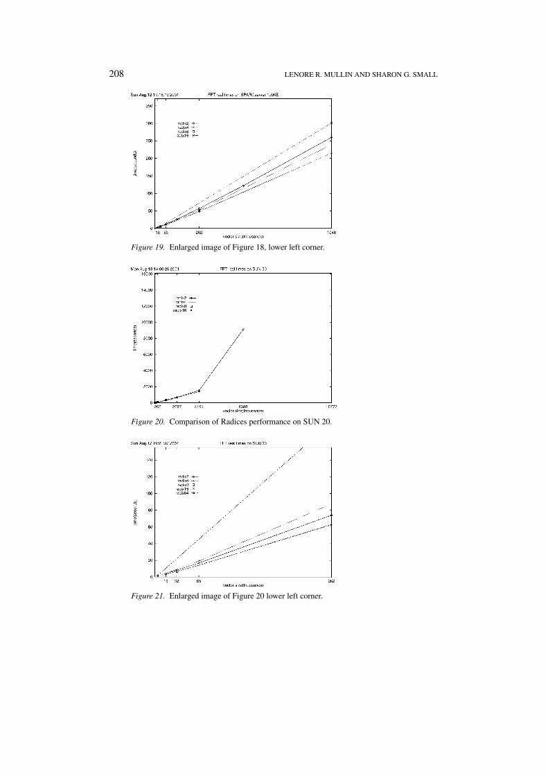
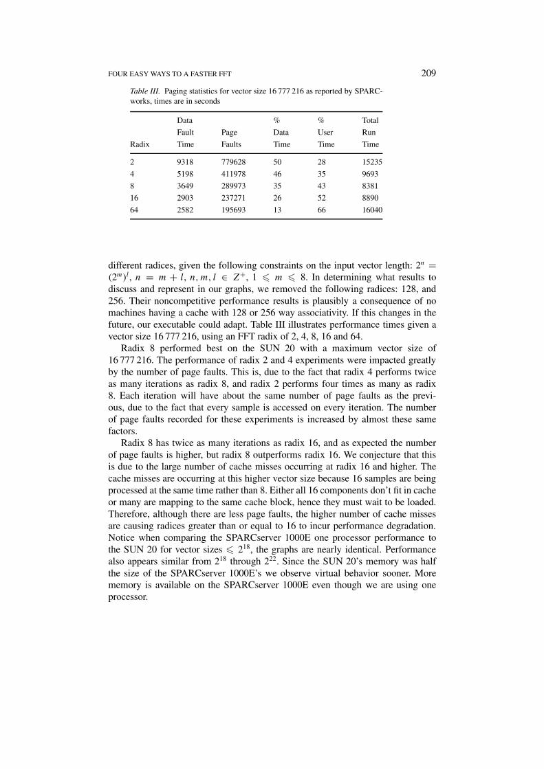
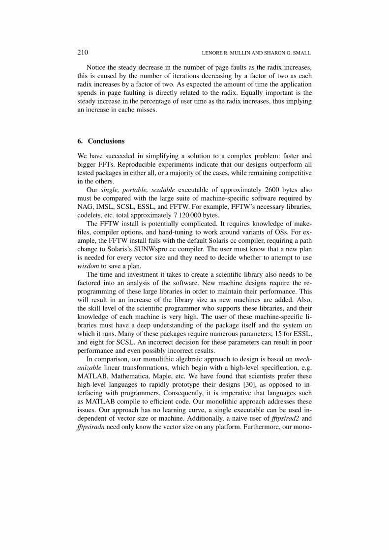
The SPARCserver 1000E and the SUN 20 (Figures 18–21) were both machinesdedicated to running our experiments. We ran our experiments for a variety of
Figure 18. Comparison of radices performance on the SUN SPARCserver 1000E: Oneprocessor.
208 LENORE R. MULLIN AND SHARON G. SMALL
Figure 19. Enlarged image of Figure 18, lower left corner.
Figure 20. Comparison of Radices performance on SUN 20.
Figure 21. Enlarged image of Figure 20 lower left corner.
FOUR EASY WAYS TO A FASTER FFT 209
Table III. Paging statistics for vector size 16 777 216 as reported by SPARC-works, times are in seconds
Data % % Total
Fault Page Data User Run
Radix Time Faults Time Time Time
2 9318 779628 50 28 15235
4 5198 411978 46 35 9693
8 3649 289973 35 43 8381
16 2903 237271 26 52 8890
64 2582 195693 13 66 16040
different radices, given the following constraints on the input vector length: 2n =(2m)l, n = m + l, n,m, l ∈ Z+, 1 � m � 8. In determining what results todiscuss and represent in our graphs, we removed the following radices: 128, and256. Their noncompetitive performance results is plausibly a consequence of nomachines having a cache with 128 or 256 way associativity. If this changes in thefuture, our executable could adapt. Table III illustrates performance times given avector size 16 777 216, using an FFT radix of 2, 4, 8, 16 and 64.
Radix 8 performed best on the SUN 20 with a maximum vector size of16 777 216. The performance of radix 2 and 4 experiments were impacted greatlyby the number of page faults. This is, due to the fact that radix 4 performs twiceas many iterations as radix 8, and radix 2 performs four times as many as radix8. Each iteration will have about the same number of page faults as the previ-ous, due to the fact that every sample is accessed on every iteration. The numberof page faults recorded for these experiments is increased by almost these samefactors.
Radix 8 has twice as many iterations as radix 16, and as expected the numberof page faults is higher, but radix 8 outperforms radix 16. We conjecture that thisis due to the large number of cache misses occurring at radix 16 and higher. Thecache misses are occurring at this higher vector size because 16 samples are beingprocessed at the same time rather than 8. Either all 16 components don’t fit in cacheor many are mapping to the same cache block, hence they must wait to be loaded.Therefore, although there are less page faults, the higher number of cache missesare causing radices greater than or equal to 16 to incur performance degradation.Notice when comparing the SPARCserver 1000E one processor performance tothe SUN 20 for vector sizes � 218, the graphs are nearly identical. Performancealso appears similar from 218 through 222. Since the SUN 20’s memory was halfthe size of the SPARCserver 1000E’s we observe virtual behavior sooner. Morememory is available on the SPARCserver 1000E even though we are using oneprocessor.
210 LENORE R. MULLIN AND SHARON G. SMALL
Notice the steady decrease in the number of page faults as the radix increases,this is caused by the number of iterations decreasing by a factor of two as eachradix increases by a factor of two. As expected the amount of time the applicationspends in page faulting is directly related to the radix. Equally important is thesteady increase in the percentage of user time as the radix increases, thus implyingan increase in cache misses.
6. Conclusions
We have succeeded in simplifying a solution to a complex problem: faster andbigger FFTs. Reproducible experiments indicate that our designs outperform alltested packages in either all, or a majority of the cases, while remaining competitivein the others.
Our single, portable, scalable executable of approximately 2600 bytes alsomust be compared with the large suite of machine-specific software required byNAG, IMSL, SCSL, ESSL, and FFTW. For example, FFTW’s necessary libraries,codelets, etc. total approximately 7 120 000 bytes.
The FFTW install is potentially complicated. It requires knowledge of make-files, compiler options, and hand-tuning to work around variants of OSs. For ex-ample, the FFTW install fails with the default Solaris cc compiler, requiring a pathchange to Solaris’s SUNWspro cc compiler. The user must know that a new planis needed for every vector size and they need to decide whether to attempt to usewisdom to save a plan.
The time and investment it takes to create a scientific library also needs to befactored into an analysis of the software. New machine designs require the re-programming of these large libraries in order to maintain their performance. Thiswill result in an increase of the library size as new machines are added. Also,the skill level of the scientific programmer who supports these libraries, and theirknowledge of each machine is very high. The user of these machine-specific li-braries must have a deep understanding of the package itself and the system onwhich it runs. Many of these packages require numerous parameters; 15 for ESSL,and eight for SCSL. An incorrect decision for these parameters can result in poorperformance and even possibly incorrect results.
In comparison, our monolithic algebraic approach to design is based on mech-anizable linear transformations, which begin with a high-level specification, e.g.MATLAB, Mathematica, Maple, etc. We have found that scientists prefer thesehigh-level languages to rapidly prototype their designs [30], as opposed to in-terfacing with programmers. Consequently, it is imperative that languages suchas MATLAB compile to efficient code. Our monolithic approach addresses theseissues. Our approach has no learning curve, a single executable can be used in-dependent of vector size or machine. Additionally, a naive user of fftpsirad2 andfftpsiradn need only know the vector size on any platform. Furthermore, our mono-
FOUR EASY WAYS TO A FASTER FFT 211
lithic algebraic approach to design is extensible to cache and other levels of thememory hierarchy, as well as parallel and distributed computing [22].
We have discovered that radix 2 is not always the best radix to choose for vectorswhose length is a power of two. This opens other interesting questions: is it betterto pad to radix 2 or use another radix�? We believe our research into a general radixformulation may yield further optimizations for FFTs.
Our research shows a systematic way of analyzing memory access patterns andsubsequent performance of the FFT on one-dimensional�� arrays whose length is2n.
Besides determining the constituent components of the sequential FFT, e.g. bitreversal or butterfly, the radix used is of paramount importance. By developingalgorithms for software, e.g., fftpsiradn, we are guaranteed that all instructions,loops and variables remain constant during the execution of the program. Hence,through monolithic analysis we can in concert, analyze the algorithm, the program,and the environment.
7. Extensions and Future Research
A goal for compilation is to be able to take a high-level specification of a scientificproblem and to realize the software mechanically, deterministically, and in lineartime. We have simulated this mechanizable method by hand for a group of algo-rithms with similar properties, namely PDE solvers, adaptive multigrids [32], LUdecomposition [11, 40], matrix multiply [31, 36], and the FFT [33]. This reportextends results of our FFT research [33, 34]. Our approach has the potential ofachieving a linear complexity when going from problem specification to efficientsoftware. Although our initial targets are transforms and algorithms with regularmemory access patterns, our results [38] using monolithic analysis indicate ourapproach applies to program blocks in general.
Our very preliminary results of the general radix research indicate choice ofradix affects performance. A goal for general radix research is to determine whatspecific machine parameters affect which radix to use. We have the ability to mod-ify the single generalized radix code into code specific to each radix, and run thesecodes experimentally on the SP-2 and Origin 2000.
References
1. Openmp simple, portable, scalable smp programming, 2000.2. Agarwal, R. C., Gustavson, F. G. and Zubair, M.: A high performance parallel algorithm for 1-
D FFT, In: Proc., Supercomputing ’94, IEEE Computer Society Press, Washington, DC, 1994,pp. 34–40.
� Padding is the usual way of handling vector lengths not equal to 2n.�� Multi-dimensional FFTs may be built from the one-dimensional FFT.
212 LENORE R. MULLIN AND SHARON G. SMALL
3. Bilmes, J., Asanovic, K., Chin, C.-W. and Demmel, J.: Optimizing matrix multiply us-ing PHiPAC: A portable, high-performance, ANSI C coding methodology, In: Proc. 1997International Conference on Supercomputing, Vienna, Austria, July 1997, pp. 340–347.
4. Center, C. M. H.: Top ten algorithms of the 20th century, Computing Science and EngineeringMagazine, 1999.
5. Chamberlain, B. L., Choi, S.-E., Lewis, C., Snyder, L., Weathersby, W. D. and Lin, C.: The casefor high-level parallel programming in ZPL, IEEE Comput. Sci. Engrg. 5(3) (1998), 76–86.
6. Chamberlain, B. L., Choi, S.-E., Lewis, E. C., Lin, C., Snyder, L. and Weathersby, W. D.:Factor-join: A unique approach to compiling array languages for parallel machines, In:D. Padua, A. Nicolau, D. Gelernter, U. Banerjee and D. Sehr (eds), Proc. Ninth InternationalWorkshop on Languages and Compilers for Parallel Computing, Lecture Notes in Comput. Sci.1239, Springer-Verlag, New York, 1996, pp. 481–500.
7. Chamberlain, B. L., Choi, S.-E. and Snyder, L.: A compiler abstraction for machine inde-pendent parallel communication generation, In: Z. Li, P. C. Yew, S. Chatterjee, C. H. Huang,P. Sadayappan and D. Sehr (eds), Languages and Compilers for Parallel Computing, LectureNotes in Comput. Sci. 1366, Springer-Verlag, New York, 1998, pp. 261–276.
8. Cormen, T.: Everything you always wanted to know about out-of-core ffts but were aftaid toask, COMPASS Colloquia Series, U Albany, SUNY, 2000.
9. Culler, D., Karp, R., Patterson, D., Sahay, A., Schauser, K. E., Santos, E., Subramonian, R.and von Eicken, T.: LogP: Toward a realistic model of parallel computation, In: Proc. FourthACM SIGPLAN Symposium on Principles and Practice of Parallel Programming, May 1993,pp. 1–12.
10. Dai, D. L., Gupta, S. K. S., Kaushik, S. D. and Lu, J. H.: EXTENT: A portable programmingenvironment for designing and implementing high-performance block-recursive algorithms, In:Proc., Supercomputing ’94, IEEE Computer Society Press, Washington, DC, 1994, pp. 49–58.
11. Dooling, D. and Mullin, L.: Indexing and distributing a general partitioned sparse array, Proc.Workshop on Solving Irregular Problems on Distributed Memory Machines, 1995.
12. Elliott, D. F. and Rao, K. R.: Fast Transforms: Algorithms, Analyses, Applications, AcademicPress, New York, 1982.
13. Frigo, M. and Johnson, S.: Fftw online documentation, Nov. 1999.14. Granata, J., Conner, M. and Tolimieri, R.: Recursive fast algorithms and the role of the tensor
product, IEEE Trans. Signal Process. 40(12) (1992), 2921–2930.15. Gupta, A. and Kumar, V.: The scalability of FFT on parallel computers, IEEE Trans. Parallel
and Distributed Systems 4(8) (1993), 922–932.16. Gupta, S., Huang, C.-H., Sadayappan, P. and Johnson, R.: On the synthesis of parallel programs
from tensor product formulas for block recursive algorithms, In: U. Banerjee, D. Gelernter,A. Nicolau and D. Padua (eds), Proc. 5th International Workshop on Languages and Com-pilers for Parallel Computing (New Haven, Connecticut), Lecture Notes in Comput. Sci. 757,Springer-Verlag, New York, 1992, pp. 264–280.
17. Gupta, S. K. S., Huang, C.-H., Sadayappan, P. and Johnson, R. W.: Implementing fastFourier transforms on distributed-memory multiprocessors using data redistributions, ParallelProcessing Lett. 4(4) (1994), 477–488.
18. Gupta, S. K. S., Huang, C.-H., Sadayappan, P. and Johnson, R. W.: A framework for generatingdistributed-memory parallel programs for block recursive algorithms, J. Parallel DistributedComput. 34(2) (1996), 137–153.
19. Hennessy, J. and Patterson, D.: Computer Architecture a Quantitative Approach, MorganKaufmann, California, 1996.
20. High Performance Fortran Forum. High Performance Fortran language specification, ScientificProgramming 2(1–2) (1993), 1–170.
21. Humphrey, W., Karmesin, S., Bassetti, F. and Reynders, J.: Optimization of data-parallelfield expressions in the POOMA framework, In: Y. Ishikawa, R. R. Oldehoeft, J. Reyn-
FOUR EASY WAYS TO A FASTER FFT 213
ders and M. Tholburn (eds), Proc. First International Conference on Scientific Computing inObject-Oriented Parallel Environments (ISCOPE ’97) (Marina del Rey, CA), Lecture Notes inComput. Sci. 1343, Springer-Verlag, New York, 1997, pp. 185–194.
22. Hunt, H., Mullin, L. and Rosenkrantz, D.: A feasibility study on the high level design ofboth sequential and parallel algorithms applied ot the fft, Paper in progress, Department ofCS SUNY, Albany, 2001.
23. Karmesin, S., Crotinger, J., Cummings, J., Haney, S., Humphrey, W., Reynders, J., Smith,S. and Williams, T.: Array design and expression evaluation in POOMA II, In: D. Caromel,R. R. Oldehoeft and M. Tholburn (eds), Proc. Second International Symposium on ScientificComputing in Object-Oriented Parallel Environments (ISCOPE ’98) (Santa Fe, NM), LectureNotes in Comput. Sci. 1505, Springer-Verlag, New York, 1998, pp.
24. Li, J. and Skjellum, A.: A poly-algorithm for parallel dense matrix multiplication on two-dimensional process grid topologies, Mississippi State Univ., 1995.
25. Lin, C. and Snyder, L.: ZPL: An array sublanguage, In: U. Banerjee, D. Gelernter, A. Nico-lau and D. Padua (eds), Proceedings of the 6th International Workshop on Languagesand Compilers for Parallel Computing (Portland, OR), Lecture Notes in Comput. Sci. 768,Springer-Verlag, New York, 1993, pp. 96–114.
26. Lumsdaine, A.: The matrix template library: A generic programming approach to high perfor-mance numerical linear algebra, In: Proceedings of International Symposium on Computing inObject-Oriented Parallel Environments, 1998.
27. Lumsdaine, A. and McCandless, B.: Parallel extensions to the matrix template library, In:Proc. 8th SIAM Conference on Parallel Processing for Scientific Computing, SIAM Press,Philadelphia, 1997.
28. Miles, D.: Compute intensity and the FFT, In: Proc., Supercomputing ’93 (Portland, OR), IEEEComputer Society Press, 1993, pp. 676–684.
29. Mullin, L.: The Psi compiler project, In: Workshop on Compilers for Parallel Computers, TUDelft, Holland, 1993.
30. Mullin, L.: On the monolithic analysis of a general radix cooley-tukey fft: Design, development,and performance, Invited talk, Lincoln Labs, MIT, 2000.
31. Mullin, L., Dooling, D., Sandberg, E. and Thibault, S.: Formal methods for portable, scalable,scheduling, routing, and communication protocol, Technical Report CSC 94-04, Dept. of CS,Univ. Missouri-Rolla, 1994.
32. Mullin, L., Kluge, W. and Scholtz, S.: On programming scientific applications in SAC – afunctional language extended by a subsystem for high level array operations, In: Proc. 8thInternational Workshop on Implementation of Functional Languages, Bonn/Germany, 1996.
33. Mullin, L. and Small, S.: Three easy steps to a faster fft (no, we don’t need a plan), Proc. 2001International Symposium on Performance Evaluation of Computer and TelecommunicationSystems, SPECTS 2001.
34. Mullin, L. and Small, S.: Three easy steps to a faster fft (the story continues...), Proc.International Conference on Imaging Science, Systems, and Technology, CISST 2001.
35. Mullin, L. M. R.: A mathematics of arrays, PhD thesis, Syracuse Univ., Dec. 1988.36. Mullin, L. R., Dooling, D., Sandberg, E. and Thibault, S.: Formal methods for scheduling,
routing and communication protocol, In: Proc. Second International Symposium on HighPerformance Distributed Computing (HPDC-2), IEEE Computer Society, 1993.
37. Mullin, L. R., Eggleston, D.,Woodrum, L. J. and Rennie, W.: The PGI–PSI project: Preprocess-ing optimizations for existing and new F90 intrinsics in HPF using compositional symmetricindexing of the Psi calculus, In: M. Gerndt (ed.), Proc. 6th Workshop on Compilers for ParallelComputers (Aachen, Germany), Forschungszentrum Jülich GmbH, 1996, pp. 345–355.
38. Rosenkrantz, D., Mullin, L. and H. B. H. III: On materializations of array-valued temporaries,In: Proc. 13th International Workshop on Languages and Compilers for Parallel Computing2000 (LCPC’00) (Yorktown Heights, NY), Springer-Verlag, New York, to be published.
214 LENORE R. MULLIN AND SHARON G. SMALL
39. Skjellum, A., Doss, N. and Bangalore, P.: Driving issues in scalable libraries: Poly-algorithms,data distribution independence, redistribution, local storage schemes, In: Proc. Seventh SIAMConference on Parallel Processing for Scientific Computing, SIAM Press, Philadelphia, 1996.
40. Thibault, S. and Mullin, L.: A pipeline implementation of LU-decomposition on a hypercube,Technical Report, Univ. Missouri-Rolla, 1994, TR 95-03.
41. Tolimieri, R., An, M. and Lu, C.: Algorithms for Discrete Fourier Tranform and Convolution,Springer-Verlag, New York, 1989.
42. Tolimieri, R., An, M. and Lu, C.: Mathematics of Multidimensional Fourier TransformAlgorithms, Springer-Verlag, New York, 1993.
43. Van Loan, C.: Computational Frameworks for the Fast Fourier Transform, Frontiers in AppliedMathematics, SIAM, Philadelphia, 1992.
44. Veldhuizen, T.: Using C++ template metaprograms, C++ Report 7(4) (1995), 36–43. Reprintedin C++ Gems (ed. Stanley Lippman).
45. Veldhuizen, T. L.: Expression templates, C++ Report 7(5) (1995), 26–31. Reprinted in C++Gems (ed. Stanley Lippman).
46. Veldhuizen, T. L.: Arrays in Blitz++, In: D. Caromel, R. R. Oldehoeft and M. Tholburn (eds),Proc. Second International Symposium on Scientific Computing in Object-Oriented ParallelEnvironments (ISCOPE ’98) (Santa Fe, NM), Lecture Notes in Comput. Sci. 1505, Springer-Verlag, New York, 1998.
47. Whaley, R. C. and Dongarra, J. J.: Automatically tuned linear algebra software, TechnicalReport UT-CS-97-366, Department of Computer Science, Univ. Tennessee, Dec. 1997.