Embed Size (px)
Citation preview
Pilot sitePilot site
Power plantsPower plants
Industrial
sources
Industrial
sources
High sand tr
end
in the F
rio
Houston
20 miles
Regional Setting of Pilot Site
Significance
to US carbon program:
Potential to
upscale to impact
US releases
International Symposium on Isotopes in Hydrology,
Marine Ecosystems, and Climate Change Studies Session 2: Carbon Dioxide Sequestration and
Related Aspects of the Carbon Cycle ----------------------------------------------------------------------------------------------------------------------------------------------------------------------------------------
Environmental impacts of geologic sequestration
of CO2: Mobilized toxic organic compounds Yousif K. Kharaka, Pamela Campbell, R. Burt Thomas
U. S. geological Survey, Menlo Park, California, USA
IAEA, Monaco, March 29, 2011
Frio Site,
Texas
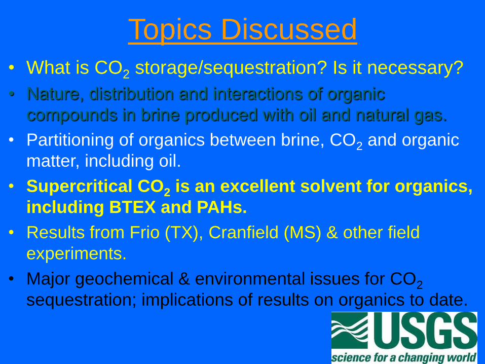
Topics Discussed
• What is CO2 storage/sequestration? Is it necessary?
• Nature, distribution and interactions of organic
compounds in brine produced with oil and natural gas.
• Partitioning of organics between brine, CO2 and organic
matter, including oil.
• Supercritical CO2 is an excellent solvent for organics,
including BTEX and PAHs.
• Results from Frio (TX), Cranfield (MS) & other field
experiments.
• Major geochemical & environmental issues for CO2
sequestration; implications of results on organics to date.
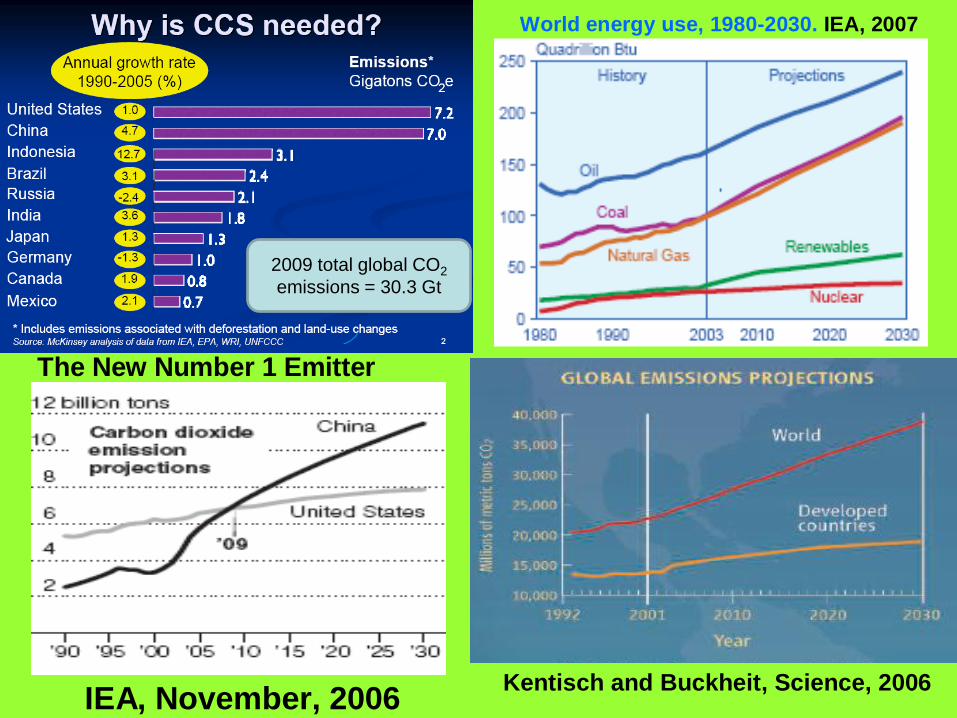
Kentisch and Buckheit, Science, 2006
The New Number 1 Emitter
World energy use, 1980-2030. IEA, 2007
IEA, November, 2006
2009 total global CO2
emissions = 30.3 Gt
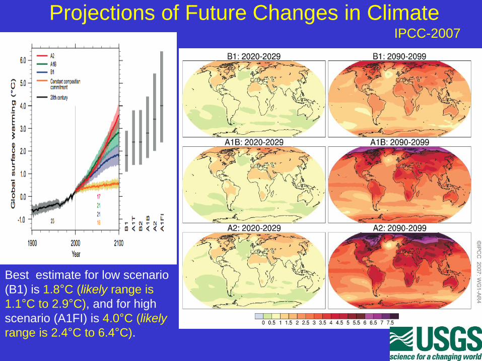
Projections of Future Changes in Climate IPCC-2007
Best estimate for low scenario
(B1) is 1.8°C (likely range is
1.1°C to 2.9°C), and for high
scenario (A1FI) is 4.0°C (likely
range is 2.4°C to 6.4°C).
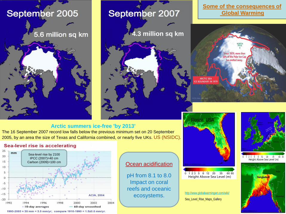
Arctic summers ice-free 'by 2013'The 16 September 2007 record low falls below the previous minimum set on 20 September
2005, by an area the size of Texas and California combined, or nearly five UKs. US (NSIDC).
4.3 million sq km
http://www.globalwarmingart.com/wiki/
Sea_Level_Rise_Maps_Gallery
Florida, USA
Some of the consequences of
Global Warming
Ocean acidification
pH from 8.1 to 8.0
Impact on coral
reefs and oceanic
ecosystems.
Sea-level rise by 2100
IPCC (2007)=40 cm
Carlson (2009)=100 cm
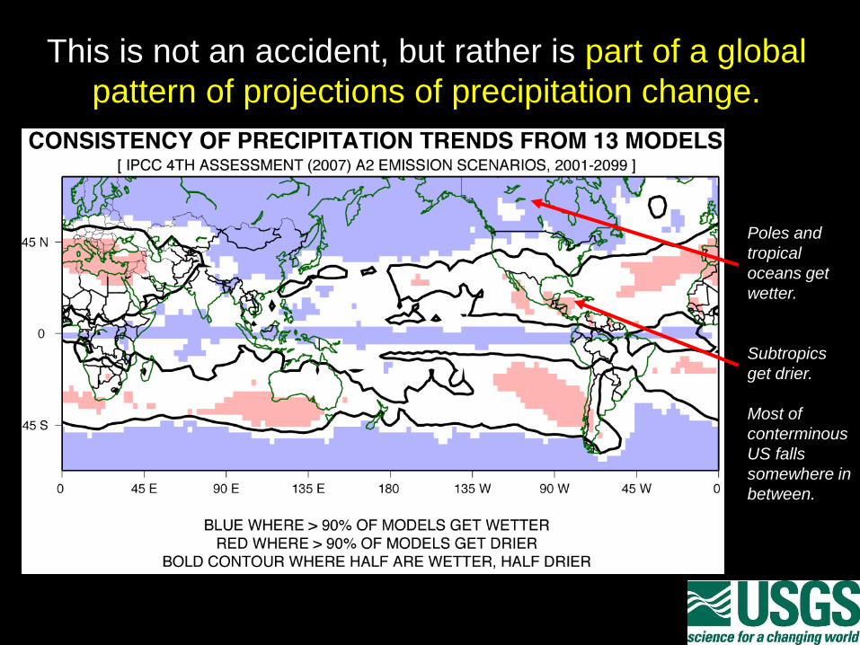
This is not an accident, but rather is part of a global
pattern of projections of precipitation change.
Poles and
tropical
oceans get
wetter.
Subtropics
get drier.
Most of
conterminous
US falls
somewhere in
between.
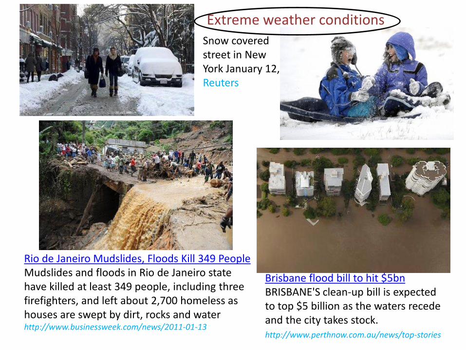
Rio de Janeiro Mudslides, Floods Kill 349 People Mudslides and floods in Rio de Janeiro state have killed at least 349 people, including three firefighters, and left about 2,700 homeless as houses are swept by dirt, rocks and water http://www.businessweek.com/news/2011-01-13
Brisbane flood bill to hit $5bn BRISBANE'S clean-up bill is expected to top $5 billion as the waters recede and the city takes stock. http://www.perthnow.com.au/news/top-stories
Snow covered street in New York January 12, Reuters
Extreme weather conditions
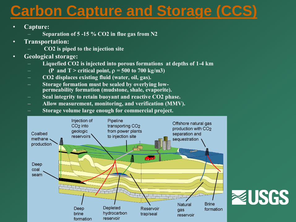
Carbon Capture and Storage (CCS)• Capture:
– Separation of 5 -15 % CO2 in flue gas from N2
• Transportation:– CO2 is piped to the injection site
• Geological storage:– Liquefied CO2 is injected into porous formations at depths of 1-4 km
– (P and T > critical point, = 500 to 700 kg/m3)
– CO2 displaces existing fluid (water, oil, gas).
– Storage formation must be sealed by overlying low-permeability formation (mudstone, shale, evaporite).
– Seal integrity to retain buoyant and reactive CO2 phase.
– Allow measurement, monitoring, and verification (MMV).
– Storage volume large enough for commercial project.
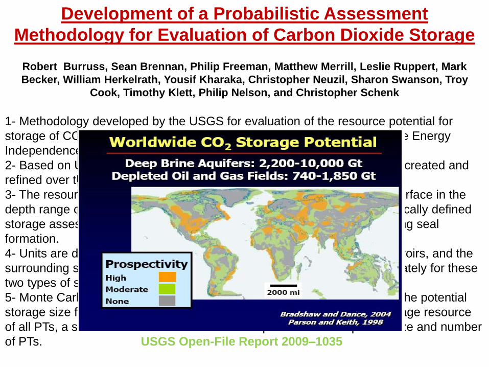
Development of a Probabilistic Assessment
Methodology for Evaluation of Carbon Dioxide Storage
Robert Burruss, Sean Brennan, Philip Freeman, Matthew Merrill, Leslie Ruppert, Mark
Becker, William Herkelrath, Yousif Kharaka, Christopher Neuzil, Sharon Swanson, Troy
Cook, Timothy Klett, Philip Nelson, and Christopher Schenk
1- Methodology developed by the USGS for evaluation of the resource potential for
storage of CO2 in the subsurface of the United States as authorized by the Energy
Independence and Security Act (Public Law 110–140, 2007).
2- Based on USGS assessment methodologies for oil and gas resources created and
refined over the last 30 years.
3- The resource that is evaluated is the volume of pore space in the subsurface in the
depth range of 3,000 to 13,000 feet that can be described within a geologically defined
storage assessment unit consisting of a storage formation and an enclosing seal
formation.
4- Units are divided into physical traps (PTs), which are oil and gas reservoirs, and the
surrounding saline formation (SF). Storage resource is determined separately for these
two types of storage.
5- Monte Carlo simulation methods are used to calculate a distribution of the potential
storage size for individual PTs and the SF. To estimate the aggregate storage resource
of all PTs, a second Monte Carlo simulation step is used to sample the size and number
of PTs. USGS Open-File Report 2009–1035
In some regions there is
mismatch between largest
sources and largest oil and
gas traps
Therefore, we need new
infrastructure, either CO2 pipelines
or new PP at storage locations
1000 MW coal PP emits 8 Mtonne/y
50 yr project = 400 Mtonne
correct for subsurface density,
convert to barrels:
4.0 BBOe at reservoir P & TFrio site
Yaqing Fan, 2006
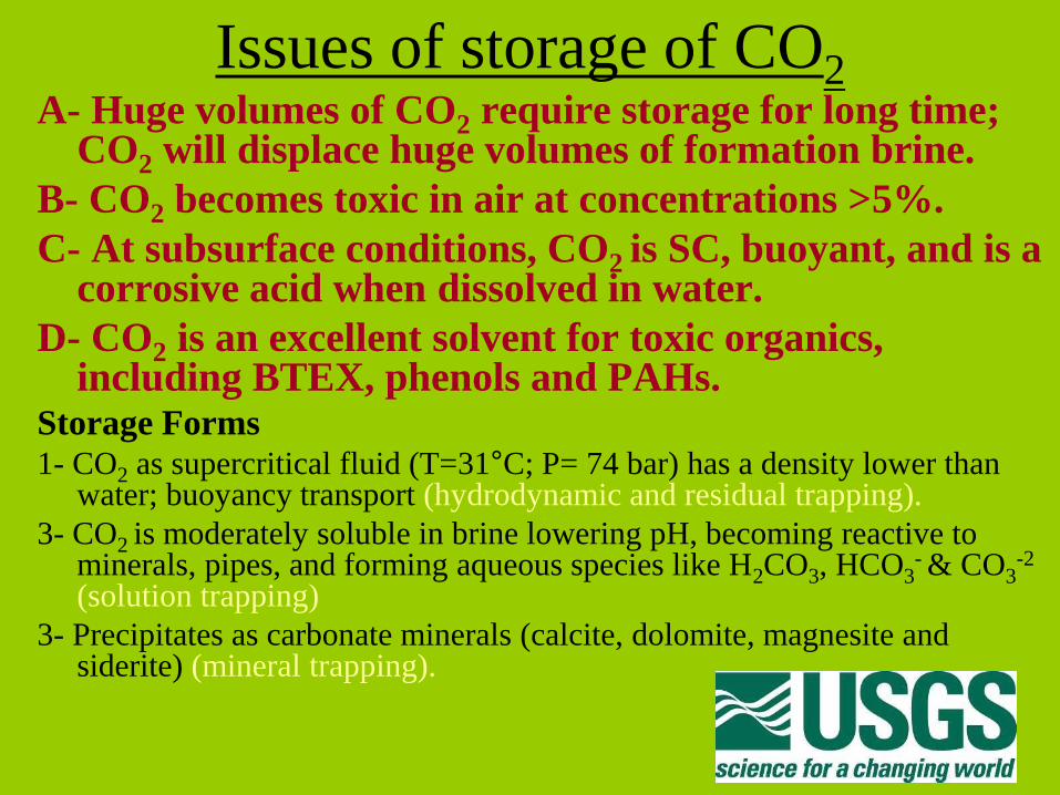
Issues of storage of CO2 A- Huge volumes of CO2 require storage for long time;
CO2 will displace huge volumes of formation brine.
B- CO2 becomes toxic in air at concentrations >5%.
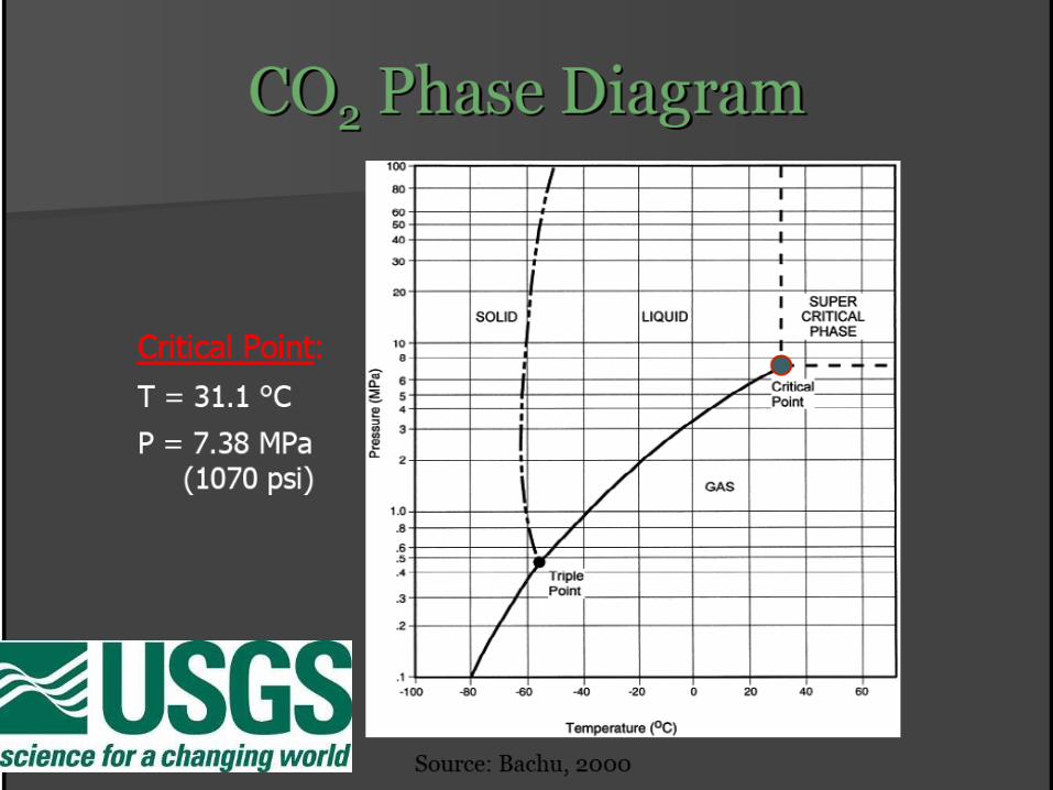
C- At subsurface conditions, CO2 is SC, buoyant, and is a corrosive acid when dissolved in water.
D- CO2 is an excellent solvent for toxic organics, including BTEX, phenols and PAHs.
Storage Forms
1- CO2 as supercritical fluid (T=31°C; P= 74 bar) has a density lower than water; buoyancy transport (hydrodynamic and residual trapping).
3- CO2 is moderately soluble in brine lowering pH, becoming reactive to minerals, pipes, and forming aqueous species like H2CO3, HCO3
- & CO3
-2 (solution trapping)
3- Precipitates as carbonate minerals (calcite, dolomite, magnesite and siderite) (mineral trapping).
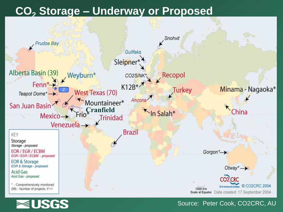
CO2 Storage – Underway or Proposed
Source: Peter Cook, CO2CRC, AU
Cranfield
Z
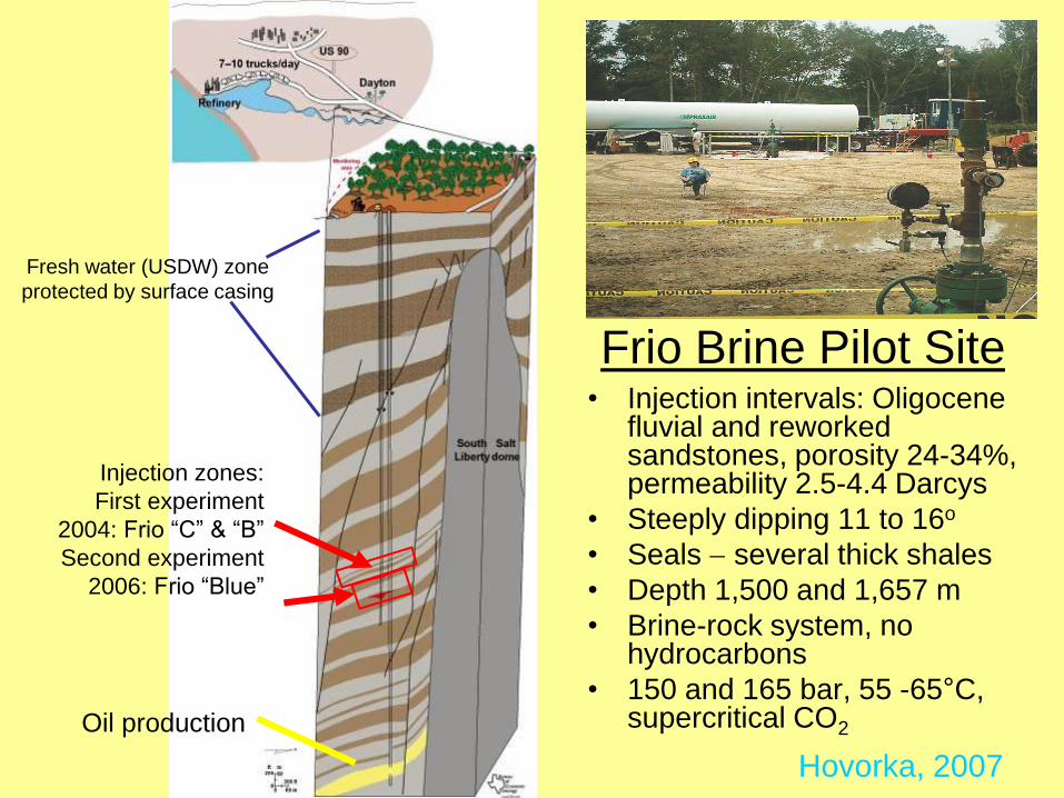
Frio Brine Pilot Site • Injection intervals: Oligocene
fluvial and reworked sandstones, porosity 24-34%, permeability 2.5-4.4 Darcys
• Steeply dipping 11 to 16o
• Seals several thick shales
• Depth 1,500 and 1,657 m
• Brine-rock system, no hydrocarbons
• 150 and 165 bar, 55 -65°C, supercritical CO2
Hovorka, 2007
Oil production
Fresh water (USDW) zone
protected by surface casing
Injection zones:
First experiment
2004: Frio ―C‖ & ―B‖
Second experiment
2006: Frio ―Blue‖
Pilot sitePilot site
Power plantsPower plants
Industrial
sources
Industrial
sources
High sand trend
in the F
rio
Houston
20 miles
Regional Setting of Pilot Site
Significance
to US carbon program:
Potential to
upscale to impact
US releases
Surface sampling
(swab) & Kuster
injection (C) &
Observation (B) wells
Jan 23-27, 2006
Surface sampling
(N2) & Kuster
injection (C) &
observation (B) wells
April 4-6, 2005
U-tubeobservation wellOct 29-Nov 3, 2004
U-tubeobservation wellOct 4-7, 2004
surface sampling
(N2), Kuster
injection &
observation wells
Jul 23-Aug 2, 2004
MDT tool
(Schlumberger)
injection wellJune 3, 2004
Sampling toolSampling site Sampling date
Surface sampling
(swab) & Kuster
injection (C) &
Observation (B) wells
Jan 23-27, 2006
Surface sampling
(N2) & Kuster
injection (C) &
observation (B) wells
April 4-6, 2005
U-tubeobservation wellOct 29-Nov 3, 2004
U-tubeobservation wellOct 4-7, 2004
surface sampling
(N2), Kuster
injection &
observation wells
Jul 23-Aug 2, 2004
MDT tool
(Schlumberger)
injection wellJune 3, 2004
Sampling toolSampling site Sampling date
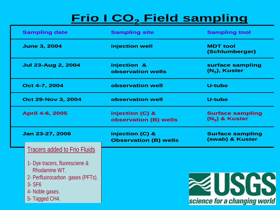
Frio I CO2 Field sampling
U-tube observation wellMarch 20, 2007
U-tube and Kusterobservation &
injection wellOct 9-10, 2006
U-tubeobservation &
injection wellsSep 25-Oct 2, 2006
surface sampling
(N2), Kuster
injection &
observation wellsSep 6-12, 2006
Sampling toolSampling site Sampling date
Frio II CO2 Field samplingTracers added to the Frio fluids
1- Dye tracers, fluoresciene & rhodamine WT; 2- perfluorocarbon tracers;
3- SF6; 4- noble gases; 5- tagged CH4
Tracers added to Frio Fluids
1- Dye tracers, fluoresciene &
Rhodamine WT.
2- Perfluorocarbon gases (PFTs).
3- SF6
4- Noble gases.
5- Tagged CH4.
Surface sampling
(swab) & Kuster
injection (C) &
Observation (B) wells
Jan 23-27, 2006
Surface sampling
(N2) & Kuster
injection (C) &
observation (B) wells
April 4-6, 2005
U-tubeobservation wellOct 29-Nov 3, 2004
U-tubeobservation wellOct 4-7, 2004
surface sampling
(N2), Kuster
injection &
observation wells
Jul 23-Aug 2, 2004
MDT tool
(Schlumberger)
injection wellJune 3, 2004
Sampling toolSampling site Sampling date
Surface sampling
(swab) & Kuster
injection (C) &
Observation (B) wells
Jan 23-27, 2006
Surface sampling
(N2) & Kuster
injection (C) &
observation (B) wells
April 4-6, 2005
U-tubeobservation wellOct 29-Nov 3, 2004
U-tubeobservation wellOct 4-7, 2004
surface sampling
(N2), Kuster
injection &
observation wells
Jul 23-Aug 2, 2004
MDT tool
(Schlumberger)
injection wellJune 3, 2004
Sampling toolSampling site Sampling date
Frio I CO2 Field sampling
U-tube observation wellMarch 20, 2007
U-tube and Kusterobservation &
injection wellOct 9-10, 2006
U-tubeobservation &
injection wellsSep 25-Oct 2, 2006
surface sampling
(N2), Kuster
injection &
observation wellsSep 6-12, 2006
Sampling toolSampling site Sampling date
Frio II CO2 Field samplingTracers added to the Frio fluids
1- Dye tracers, fluoresciene & rhodamine WT; 2- perfluorocarbon tracers;
3- SF6; 4- noble gases; 5- tagged CH4
U-tube observation wellMarch 20, 2007
U-tube and Kusterobservation &
injection wellOct 9-10, 2006
U-tubeobservation &
injection wellsSep 25-Oct 2, 2006
surface sampling
(N2), Kuster
injection &
observation wellsSep 6-12, 2006
Sampling toolSampling site Sampling date
Frio II CO2 Field samplingTracers added to the Frio fluids
1- Dye tracers, fluoresciene & rhodamine WT; 2- perfluorocarbon tracers;
3- SF6; 4- noble gases; 5- tagged CH4
Tracers added to Frio Fluids
1- Dye tracers, fluoresciene &
Rhodamine WT.
2- Perfluorocarbon gases (PFTs).
3- SF6
4- Noble gases.
5- Tagged CH4.
5.5
5.7
5.9
6.1
6.3
6.5
6.7
6.9
4-Oct-04 5-Oct-04 6-Oct-04 7-Oct-04 8-Oct-04
pH
0
500
1000
1500
2000
2500
3000
3500
Alk
alin
ity
HC
O3 (
mg
/L);
EC
(x
10
mS
/cm
)
pH
HCO3
EC
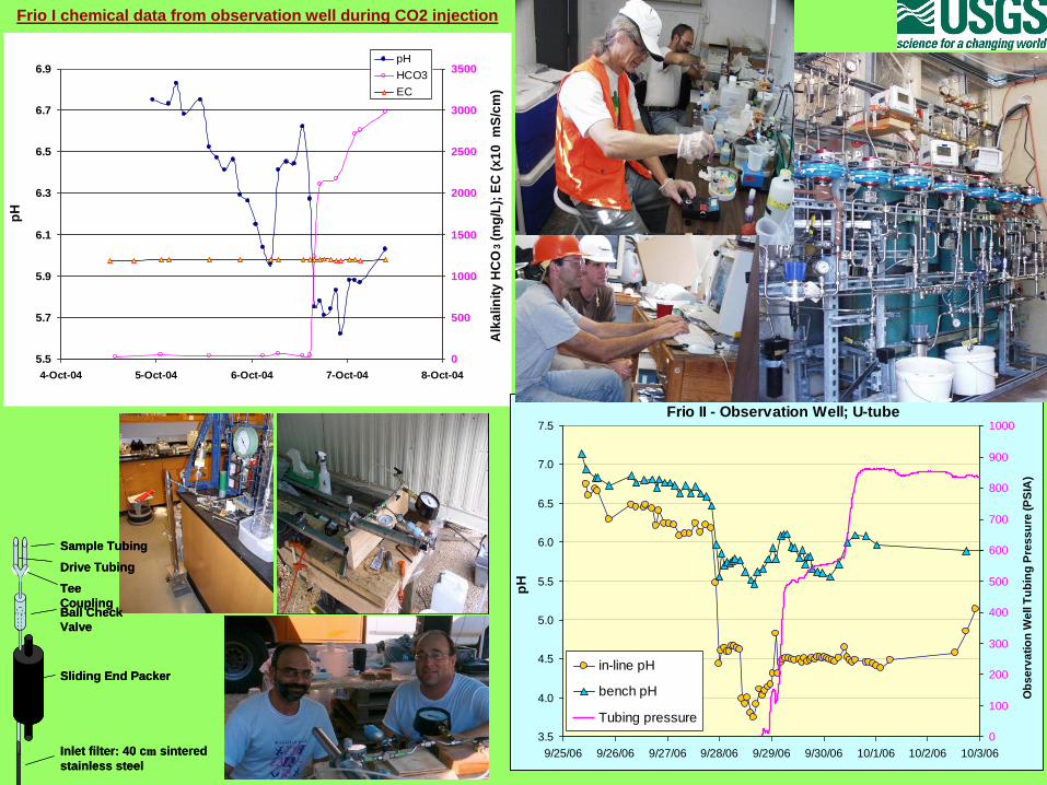
Frio I chemical data from observation well during CO2 injection
Frio II - Observation Well; U-tube
3.5
4.0
4.5
5.0
5.5
6.0
6.5
7.0
7.5
9/25/06 9/26/06 9/27/06 9/28/06 9/29/06 9/30/06 10/1/06 10/2/06 10/3/06
pH
0
100
200
300
400
500
600
700
800
900
1000
Ob
se
rva
tio
n W
ell T
ub
ing
Pre
ss
ure
(P
SIA
)
in-line pH
bench pH
Tubing pressure
Ball Check
Valve
Inlet filter: 40 cm sintered
stainless steel
Tee
Coupling
Sliding End Packer
Sample Tubing
Drive Tubing
Ball Check
Valve
Inlet filter: 40 cm sintered
stainless steel
Tee
Coupling
Sliding End Packer
Sample Tubing
Drive Tubing
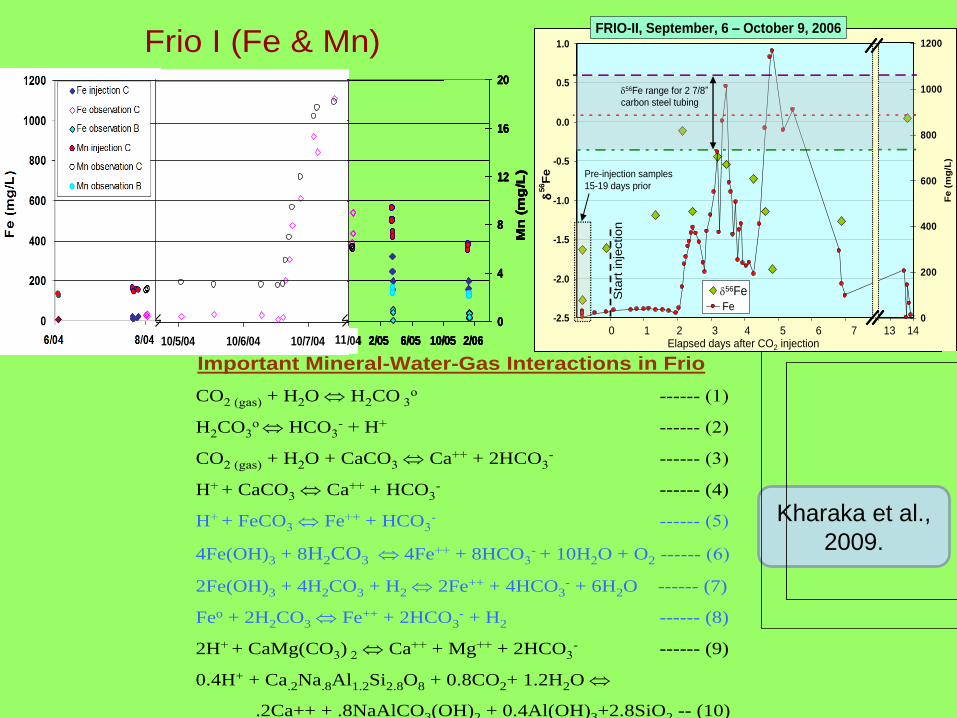
Frio I (Fe & Mn)
― ‖
― ‖
― ‖
― ‖
― ‖
― ‖
0
200
400
600
800
1000
1200
10/4/04 10/5/04 10/6/04 10/7/04 10/8/04
0
4
8
12
16
20
0
200
400
600
800
1000
1200
10/04 2/05 6/05 10/05 2/06
0
4
8
12
16
20
Mn
(m
g/L
)
11
0
200
400
600
800
1000
1200
10/4/04 10/5/04 10/6/04 10/7/04 10/8/04
0
4
8
12
16
20
0
200
400
600
800
1000
1200
10/04 2/05 6/05 10/05 2/06
0
4
8
12
16
20
Mn
(m
g/L
)
0
200
400
600
800
1000
1200
10/4/04 10/5/04 10/6/04 10/7/04 10/8/04
0
4
8
12
16
20
0
200
400
600
800
1000
1200
10/04 2/05 6/05 10/05 2/06
0
4
8
12
16
20
Mn
(m
g/L
)
0
200
400
600
800
1000
1200
10/4/04 10/5/04 10/6/04 10/7/04 10/8/04
0
4
8
12
16
20
0
200
400
600
800
1000
1200
10/4/04 10/5/04 10/6/04 10/7/04 10/8/04
0
4
8
12
16
20
0
200
400
600
800
1000
1200
10/04 2/05 6/05 10/05 2/06
0
4
8
12
16
20
Mn
(m
g/L
)
11
Eh-pH diagram for selected Fe species
Important Mineral-Water-Gas Interactions in Frio
CO2 (gas) + H2O H2CO 3o ------ (1)
H2CO3o HCO3
- + H+ ------ (2)
CO2 (gas) + H2O + CaCO3 Ca++ + 2HCO3- ------ (3)
H+ + CaCO3 Ca++ + HCO3- ------ (4)
H+ + FeCO3 Fe++ + HCO3- ------ (5)
4Fe(OH)3 + 8H2CO3 4Fe++ + 8HCO3- + 10H2O + O2 ------ (6)
2Fe(OH)3 + 4H2CO3 + H2 2Fe++ + 4HCO3- + 6H2O ------ (7)
Feo + 2H2CO3 Fe++ + 2HCO3- + H2 ------ (8)
2H+ + CaMg(CO3) 2 Ca++ + Mg++ + 2HCO3- ------ (9)
0.4H+ + Ca.2Na.8Al1.2Si2.8O8 + 0.8CO2+ 1.2H2O
.2Ca++ + .8NaAlCO3(OH)2 + 0.4Al(OH)3+2.8SiO2 -- (10)
Kharaka et al.,
2009.
-2.5
-2.0
-1.5
-1.0
-0.5
0.0
0.5
1.0
-24 0 24 48 72 96 120 144 168 192 216
Elapsed Hours after CO2 Injection
Fe/Z
n (
wt)
0
50
100
150
200
250
300
350
d56F
e
56Fe
Fe/Zn
-2.5
-2.0
-1.5
-1.0
-0.5
0.0
0.5
1.0
48 72 96 120 144 168 192 216 240 264 288 312 336
Elapsed Hours after CO2 Injection
Fe/Z
n (
wt)
0
50
100
150
200
250
300
350
d56F
e
56Fe
Fe/Zn
d56Fe range for 2 7/8‖
carbon steel tubing
Sta
rt
inje
ction
Pre-injection samples
15-19 days prior
Elapsed days after CO2 injection
0 1 2 3 4 5 6 7 8 13 14
d56Fe
FRIO-II, September, 6 – October 9, 2006
Fe/Zn from pipes: 20-45 x 103
-2.5
-2.0
-1.5
-1.0
-0.5
0.0
0.5
1.0
-24 0 24 48 72 96 120 144 168 192
Elapsed Hours after CO2 Injection
Fe/M
n (
wt)
0
10
20
30
40
50
60
70
80
90
100
d56F
e
56Fe
Fe/Mn
-2.5
-2.0
-1.5
-1.0
-0.5
0.0
0.5
1.0
48 72 96 120 144 168 192 216 240 264 288 312 336
Elapsed Hours after CO2 Injection
Fe/M
n (
wt)
0
10
20
30
40
50
60
70
80
90
100
d56F
e
56Fe
Fe/Mn
d56Fe range for 2 7/8‖
carbon steel tubing
Sta
rt
inje
ctio
n
Pre-injection samples
15-19 days prior
Elapsed days after CO2 injection0 1 2 3 4 5 6 7 13 14
d56Fe
FRIO-II, September, 6 – October 9, 2006
Fe/Mn from pipes 63-91
-2.5
-2.0
-1.5
-1.0
-0.5
0.0
0.5
1.0
-24 0 24 48 72 96 120 144 168 192
Elapsed Days after CO2 Injection
Fe
(m
g/L
)
0
200
400
600
800
1000
1200
d56F
e
56Fe
Fe
Frio II
-2.5
-2.0
-1.5
-1.0
-0.5
0.0
0.5
1.0
0 24 48 72 96 120 144 168 192 216 240 264 288 312 336
Elapsed Hours after CO2 Injection
Fe
(m
g/L
)
0
200
400
600
800
1000
1200
d56F
e
56Fe
Fe
d56Fe range for 2 7/8‖
carbon steel tubing
Sta
rt inje
ction
Pre-injection samples
15-19 days prior
Elapsed days after CO2 injection0 1 2 3 4 5 6 7 13 14
d56Fe
-2.5
-2.0
-1.5
-1.0
-0.5
0.0
0.5
1.0
-24 0 24 48 72 96 120 144 168 192
Elapsed Days after CO2 Injection
Fe
(m
g/L
)
0
200
400
600
800
1000
1200
d56F
e
56Fe
Fe
Frio II
-2.5
-2.0
-1.5
-1.0
-0.5
0.0
0.5
1.0
0 24 48 72 96 120 144 168 192 216 240 264 288 312 336
Elapsed Hours after CO2 Injection
Fe
(m
g/L
)
0
200
400
600
800
1000
1200
d56F
e
56Fe
Fe
d56Fe range for 2 7/8‖
carbon steel tubing
Sta
rt inje
ction
Pre-injection samples
15-19 days prior
Elapsed days after CO2 injection0 1 2 3 4 5 6 7 13 14
-2.5
-2.0
-1.5
-1.0
-0.5
0.0
0.5
1.0
-24 0 24 48 72 96 120 144 168 192
Elapsed Days after CO2 Injection
Fe
(m
g/L
)
0
200
400
600
800
1000
1200
d56F
e
56Fe
Fe
Frio II
-2.5
-2.0
-1.5
-1.0
-0.5
0.0
0.5
1.0
0 24 48 72 96 120 144 168 192 216 240 264 288 312 336
Elapsed Hours after CO2 Injection
Fe
(m
g/L
)
0
200
400
600
800
1000
1200
d56F
e
56Fe
Fe
d56Fe range for 2 7/8‖
carbon steel tubing
Sta
rt inje
ction
Pre-injection samples
15-19 days prior
Elapsed days after CO2 injection0 1 2 3 4 5 6 7 13 14
d56Fe
FRIO-II, September, 6 – October 9, 2006

I
Benson & Cook, 2005;
IPCC, 2005
A- Huge volumes of CO2 require storage for long time; CO2 will displace huge
volumes of formation water.
B- CO2 is non toxic, but will displace air & is buoyant and reactive in the subsurface.
Storage Forms1- CO2 as supercritical fluid (T=31°C; P= 74 bar) has a density lower than water;
buoyancy transport (hydrodynamic & residual trapping).
2- CO2 is moderately soluble in brine lowering pH and forming aqueous species like
H2CO3, HCO3- and CO3
—2 (solution trapping).
3- Precipitates as carbonate minerals (calcite, dolomite, magnesite & siderite) (mineral trapping).
Storage of CO2
0 20 40 60 80 100 120 140 1602
3
4
5
6
7
pH
pCO2 (bars)
pH
-12
-10
-8
-6
-4
-2
0
2
4pH values at:
surface
T & P
eq. calcite
calcite
albite, low
dolomite
goethite
siderite
G
(kca
l/mol
e)
Computer SimulationsTo understand
gas-water-mineral
Interactions and
multi phase fluid transport
Benson & Cook, 2005
100 75 50 25 0 25 50 75 100
Frio II "blue" sand [06FCO2-212]
(observation well; pre-injection)
100 75 50 25 0 25 50 75 100
Frio I "C" sand [04FCO2-218]
(observation well, pre-injection)
100 75 50 25 0 25 50 75 100
[milliequivalents/liter, normalized to 100%]
pH = 6.7; TDS = 93,800 mg/L
pH = 6.6; TDS = 92,200 mg/LpH = 6.03; TDS = 92,600 mg/L
pH = 6.7; TDS = 101,600 mg/L
Cl Cl
Cl Cl
SO4
SO4SO
4
HCO3
HCO3
HCO3
Mg
HCO3
SO4
MgMg
Mg
Ca
CaCa
Na
Na
Na
Ca
Na
Frio I "C" sand [04FCO2-337]
(observation well; post injection)
100 75 50 25 0 25 50 75 100
Frio "B" sand [05FCO2-110]
(observation well)
Audigane et al. (2008)
Benson & Cook (2005)
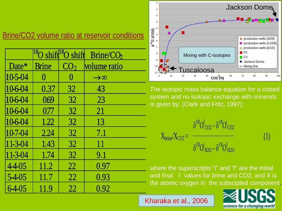
Brine/CO2 volume ratio at reservoir conditions
18O shift18O shift Brine/CO 2Date* Brine CO 2 volume ratio
10-5-04 0 0
10-6-04 0.37 32 43
10-6-04 0.69 32 23
10-6-04 0.77 32 21
10-6-04 1.22 32 13
10-7-04 2.24 32 7.1
11-3-04 1.43 32 11
11-3-04 1.74 32 9.1
4-4-05 11.2 22 0.97
5-4-05 11.7 22 0.93
6-4-05 11.9 22 0.92
18O shift18O shift Brine/CO 2Date* Brine CO 2 volume ratio
10-5-04 0 0
10-6-04 0.37 32 43
10-6-04 0.69 32 23
10-6-04 0.77 32 21
10-6-04 1.22 32 13
18O shift18O shift Brine/CO 2Date* Brine CO 2 volume ratio
10-5-04 0 0
10-6-04 0.37 32 43
10-6-04 0.69 32 23
10-6-04 0.77 32 21
10-6-04 1.22 32 13
10-7-04 2.24 32 7.1
11-3-04 1.43 32 11
11-3-04 1.74 32 9.1
4-4-05 11.2 22 0.97
5-4-05 11.7 22 0.93
6-4-05 11.9 22 0.92
d18
OfCO2 - d
18O
iCO2
Xbrine/XCO2 = _______________________
(1)
d18
OiH2O - d
18O
fH2O
The isotopic mass balance equation for a closed
system and no isotopic exchange with minerals
is given by: (Clark and Fritz, 1997):
where the superscripts ―i‖ and ―f‖ are the initial
and final δ values for brine and CO2, and X is
the atomic oxygen in the subscipted component.
Kharaka et al., 2006
-11
-10
-9
-8
-7
-6
-5
-4
-3
-2
-1
0
0 10 20 30 40 50 60 70 80 90 100
CO2 (%)
d1
3C
(C
O2
)
production wells [3/09]
production wells [12/09]
production wells [4/10]
F2
F3
Jackson Dome
Mixing line
Jackson Dome
Tuscaloosa
Mixing with C-isotopes
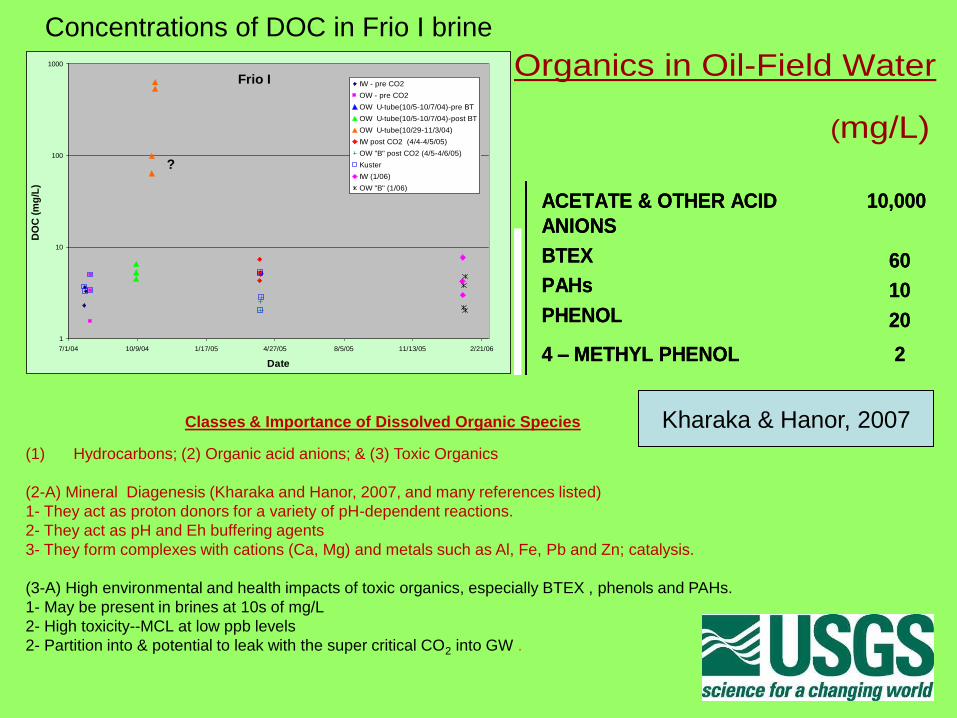
Concentrations of DOC in Frio I brine
Frio I
1
10
100
1000
7/1/04 10/9/04 1/17/05 4/27/05 8/5/05 11/13/05 2/21/06
Date
DO
C (
mg
/L)
IW - pre CO2
OW - pre CO2
OW U-tube(10/5-10/7/04)-pre BT
OW U-tube(10/5-10/7/04)-post BT
OW U-tube(10/29-11/3/04)
IW post CO2 (4/4-4/5/05)
OW "B" post CO2 (4/5-4/6/05)
Kuster
IW (1/06)
OW "B" (1/06)
?
0.00
1.00
2.00
3.00
4.00
5.00
6.00
7.00
8.00
9.00
10.00
0 500 1000 1500 2000 2500 3000 3500
HCO3
DO
C
OW-pre
IW-pre
slugtest
OW-pre BT
OW-post BT
OW-10/9
OW-K 10/9/06
OW-11/2/06
IW-U
IW-K
Frio II
Organics in Oil-Field Water
(mg/L)
Frio DOC (6/04-4/05)
0
1
10
100
1000
Jun-04 Aug-04 Oct-04 Dec-04 Feb-05 Apr-05
DO
C (
mg
/L)
DOC injection w ell
DOC observation w ell C-sand
DOC observation w ell B-sand
Organics in Produced Water
(mg/L)
0.7Ground Water
7Surface Water
5-1000Produced Water
MeanDOC
0.7Ground Water
7Surface Water
5-1000Produced Water
MeanDOC
Kharaka & Hanor, 2004
1.23 – HYDROXY BENZOIC ACID
0.22 – HYROXY BENZOIC ACID
44 – METHYL BENZOIC ACID
5BENZOIC ACID
24 – METHYL PHENOL
10,000
60
10
20
ACETATE & OTHER ACID
ANIONS
BTEX
PAHs
PHENOL
Kharaka & Hanor, 2004
1.23 – HYDROXY BENZOIC ACID
0.22 – HYROXY BENZOIC ACID
44 – METHYL BENZOIC ACID
5BENZOIC ACID
24 – METHYL PHENOL
10,000
60
10
20
ACETATE & OTHER ACID
ANIONS
BTEX
PAHs
PHENOL
Kharaka & Hanor, 2007 Classes & Importance of Dissolved Organic Species
(1) Hydrocarbons; (2) Organic acid anions; & (3) Toxic Organics
(2-A) Mineral Diagenesis (Kharaka and Hanor, 2007, and many references listed)
1- They act as proton donors for a variety of pH-dependent reactions.
2- They act as pH and Eh buffering agents
3- They form complexes with cations (Ca, Mg) and metals such as Al, Fe, Pb and Zn; catalysis.
(3-A) High environmental and health impacts of toxic organics, especially BTEX , phenols and PAHs.
1- May be present in brines at 10s of mg/L
2- High toxicity--MCL at low ppb levels
2- Partition into & potential to leak with the super critical CO2 into GW .
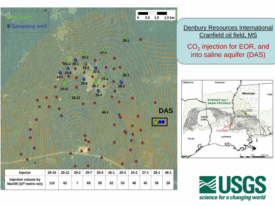
Sampling well
24-3
29-3
29-1
29-6
29-5
29-9
29-2
29-7
26-1
25-2
24-2
29-4
27-1
48-1
28-2
28-1
29-12
29-10
Injector 29-10 29-12 29-2 29-7 29-4
69 587
26-1 25-2 24-2 27-1 28-1 48-1
Injection volume byMar/09 (103 metric ton) 110 62 52 53 48 45 56 28
Injector 0 0.5 1.0 1.5 km
DAS
0 125 250 km
Jackson Dome
Denbury Resources International
Cranfield oil field, MS
CO2 injection for EOR, and
into saline aquifer (DAS)
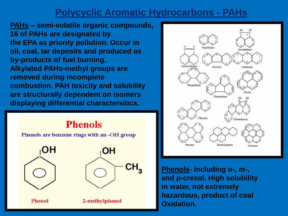
Polycyclic Aromatic Hydrocarbons - PAHs
PAHs – semi-volatile organic compounds,
16 of PAHs are designated by
the EPA as priority pollution. Occur in
oil, coal, tar deposits and produced as
by-products of fuel burning.
Alkylated PAHs-methyl groups are
removed during incomplete
combustion. PAH toxicity and solubility
are structurally dependent on isomers
displaying differential charactersitics.
Phenols- including o-, m-,
and p-cresol. High solubility
in water, not extremely
hazardous, product of coal
Oxidation.
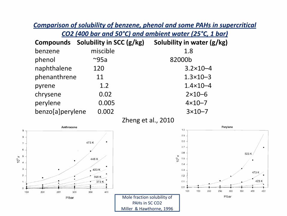
Comparison of solubility of benzene, phenol and some PAHs in supercritical CO2 (400 bar and 50°C) and ambient water (25°C, 1 bar)
Compounds Solubility in SCC (g/kg) Solubility in water (g/kg) benzene miscible 1.8 phenol ~95a 82000b naphthalene 120 3.2×10⁻⁴ phenanthrene 11 1.3×10⁻³ pyrene 1.2 1.4×10⁻⁴ chrysene 0.02 2×10⁻⁶ perylene 0.005 4×10⁻⁷ benzo[a]perylene 0.002 3×10⁻⁷ Zheng et al., 2010
Mole fraction solubility of PAHs in SC CO2
Miller & Hawthorne, 1996
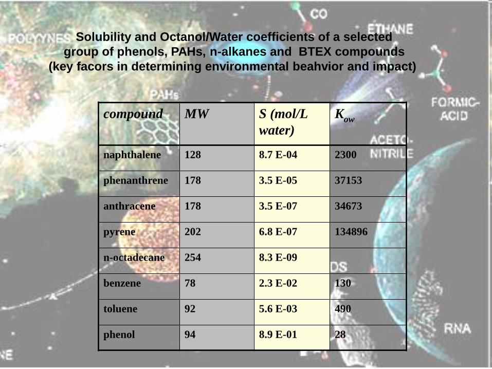
22
compound MW S (mol/L
water)
Kow
naphthalene 128 8.7 E-04 2300
phenanthrene 178 3.5 E-05 37153
anthracene 178 3.5 E-07 34673
pyrene 202 6.8 E-07 134896
n-octadecane 254 8.3 E-09
benzene 78 2.3 E-02 130
toluene 92 5.6 E-03 490
phenol 94 8.9 E-01 28
Solubility and Octanol/Water coefficients of a selected
group of phenols, PAHs, n-alkanes and BTEX compounds
(key facors in determining environmental beahvior and impact)
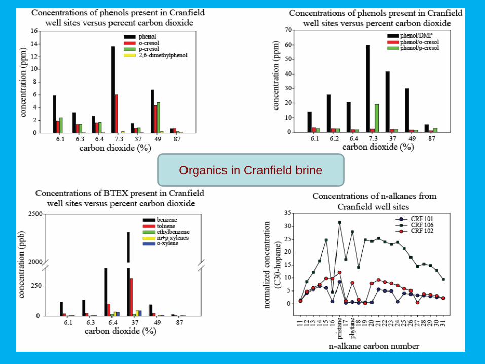
Organics in Cranfield brine
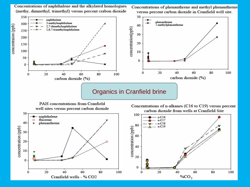
Organics in Cranfield brine
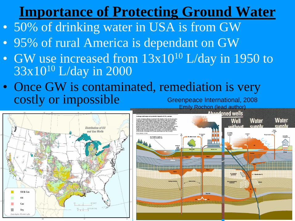
• 50% of drinking water in USA is from GW
• 95% of rural America is dependant on GW
• GW use increased from 13x1010 L/day in 1950 to 33x1010 L/day in 2000
• Once GW is contaminated, remediation is very costly or impossible
Importance of Protecting Ground Water
Greenpeace International, 2008Emily Rochon (lead author)
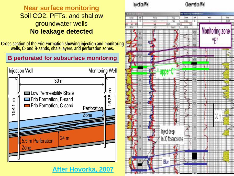
Cross section of the Frio Formation showing injection and monitoring wells, C- and B-sands, shale layers, and perforation zones.
B perforated for subsurface monitoring
After Hovorka, 2007
Near surface monitoring
Soil CO2, PFTs, and shallow
groundwater wells
No leakage detected
B perforated for subsurface monitoring
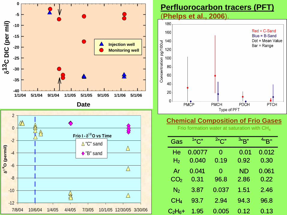
Date
1/1/04 5/1/04 9/1/04 1/1/05 5/1/05 9/1/05 1/1/06 5/1/06
d13C
DIC
(p
er
mil)
-40
-35
-30
-25
-20
-15
-10
-5
0
Injection well
Monitoring well
Frio I - d18
O vs Time
-12
-10
-8
-6
-4
-2
0
2
7/8/04 10/6/04 1/4/05 4/4/05 7/3/05 10/1/05 12/30/05 3/30/06
d1
8O
(p
erm
il) "C" sand
"B" sand
Chemical Composition of Frio GasesFrio formation water at saturation with CH4
Gas1‖C‖
2‖C‖
3―B‖
4"B"
He 0.0077 0 0.01 0.012
H2 0.040 0.19 0.92 0.30
Ar 0.041 0 ND 0.061
CO2 0.31 96.8 2.86 0.22
N2 3.87 0.037 1.51 2.46
CH4 93.7 2.94 94.3 96.8
C2H6+ 1.95 0.005 0.12 0.13
Gas1‖C‖
2‖C‖
3―B‖
4"B"
He 0.0077 0 0.01 0.012
H2 0.040 0.19 0.92 0.30
Ar 0.041 0 ND 0.061
CO2 0.31 96.8 2.86 0.22
N2 3.87 0.037 1.51 2.46
CH4 93.7 2.94 94.3 96.8
C2H6+ 1.95 0.005 0.12 0.13
Perfluorocarbon tracers (PFT)(Phelps et al., 2006).
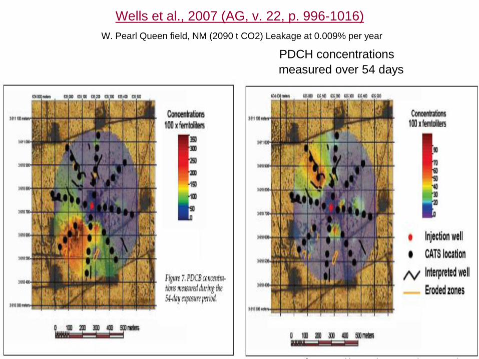
Wells et al., 2007 (AG, v. 22, p. 996-1016)
W. Pearl Queen field, NM (2090 t CO2) Leakage at 0.009% per year
PDCH concentrations
measured over 54 days
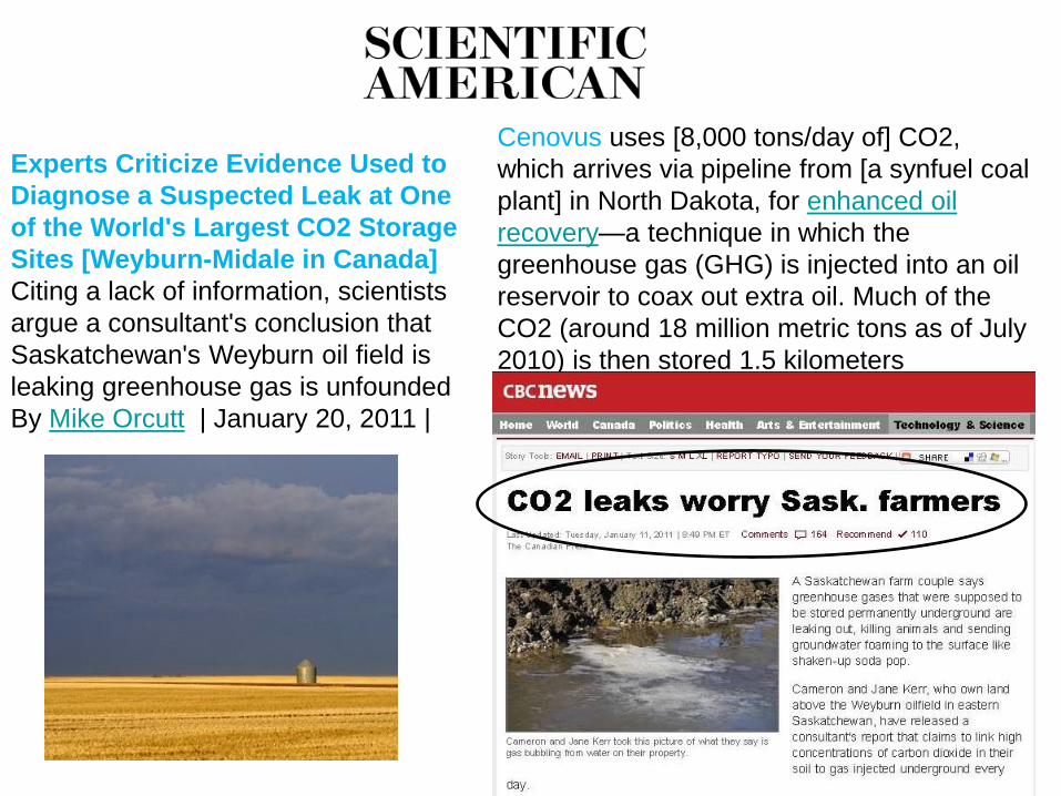
Experts Criticize Evidence Used to
Diagnose a Suspected Leak at One
of the World's Largest CO2 Storage
Sites [Weyburn-Midale in Canada]
Citing a lack of information, scientists
argue a consultant's conclusion that
Saskatchewan's Weyburn oil field is
leaking greenhouse gas is unfounded
By Mike Orcutt | January 20, 2011 |
Cenovus uses [8,000 tons/day of] CO2,
which arrives via pipeline from [a synfuel coal
plant] in North Dakota, for enhanced oil
recovery—a technique in which the
greenhouse gas (GHG) is injected into an oil
reservoir to coax out extra oil. Much of the
CO2 (around 18 million metric tons as of July
2010) is then stored 1.5 kilometers
underground in a depleted reservoir, where it
is supposed to stay trapped. The
International Energy Agency (IEA) GHG
Weyburn–Midale CO2 Monitoring and
Storage Project, a research group affiliated
with the Paris-based agency has spent the
past decade studying CO2 injection and
storage at Weyburn, the goal being to
"deliver the framework necessary to
encourage implementation of CO2 geological
storage on a worldwide basis," according to
the group's web site.
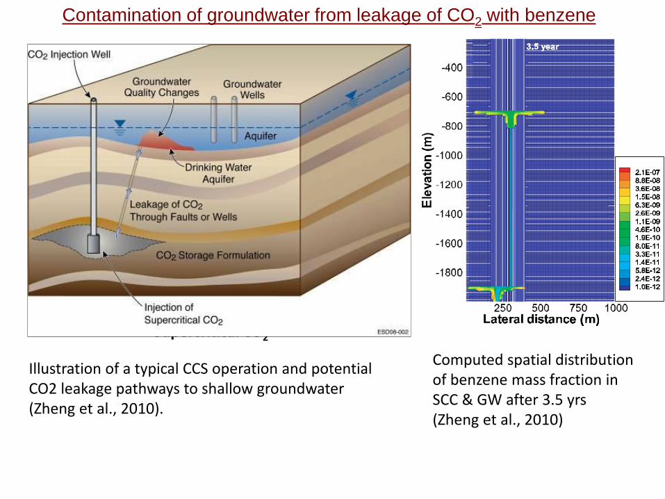
Illustration of a typical CCS operation and potential CO2 leakage pathways to shallow groundwater (Zheng et al., 2010).
Injection of Supercritical CO2
CO2 storage formation
Computed spatial distribution of benzene mass fraction in SCC & GW after 3.5 yrs (Zheng et al., 2010)
Contamination of groundwater from leakage of CO2 with benzene
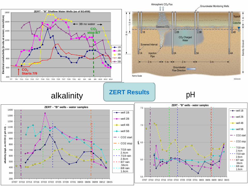
pH ZERT - "B" wells - water samples
5.5
6.0
6.5
7.0
7.5
07/07 07/10 07/13 07/16 07/19 07/22 07/25 07/28 07/31 08/03 08/06 08/09 08/12 08/15
pH
.
well 1B
well 2B
well 4B
well 5B
CO2 start
CO2 stop
7/18 rain2.4cm7/19 rain2.8cm8/7 rain.56cm8/8 rain1.6cm
alkalinityZERT - "B" wells - water samples
200
300
400
500
600
700
800
900
1000
1100
1200
1300
1400
07/07 07/10 07/13 07/16 07/19 07/22 07/25 07/28 07/31 08/03 08/06 08/09 08/12 08/15
alk
alin
ity
(m
g/L
as
HC
O3
@ p
H 4
.5)
.
well 1B
well 2B
well 4B
well 5B
CO2 start
CO2 stop
7/18 rain2.4cm7/19 rain2.8cm8/7 rain.56cm8/8 rain1.6cm
ZERT Results
ZERT - "B" Shallow Water Wells (as of 8/14/08)
400
600
800
1000
1200
1400
1600
1800
7/7 7/9 7/11 7/13 7/15 7/17 7/19 7/21 7/23 7/25 7/27 7/29 7/31 8/2 8/4 8/6 8/8 8/10 8/12 8/14
Ele
ctr
ica
l co
nd
uc
tiv
ity
(in
-sit
u a
t s
cre
en
; m
icro
S/c
m)
1B
2B
3B
4B
5B
3B no water
CO2
stop 8/7
CO2
Starts 7/9
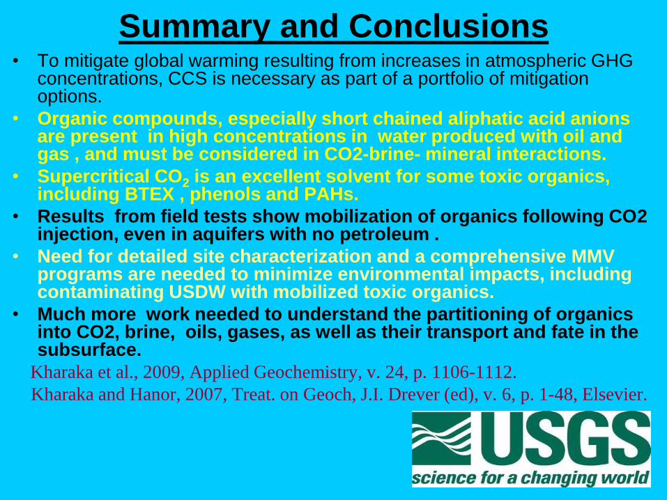
• To mitigate global warming resulting from increases in atmospheric GHG concentrations, CCS is necessary as part of a portfolio of mitigation options.
• Organic compounds, especially short chained aliphatic acid anions are present in high concentrations in water produced with oil and gas , and must be considered in CO2-brine- mineral interactions.
• Supercritical CO2 is an excellent solvent for some toxic organics, including BTEX , phenols and PAHs.
• Results from field tests show mobilization of organics following CO2 injection, even in aquifers with no petroleum .
• Need for detailed site characterization and a comprehensive MMV programs are needed to minimize environmental impacts, including contaminating USDW with mobilized toxic organics.
• Much more work needed to understand the partitioning of organics into CO2, brine, oils, gases, as well as their transport and fate in the subsurface.
Kharaka et al., 2009, Applied Geochemistry, v. 24, p. 1106-1112.
Kharaka and Hanor, 2007, Treat. on Geoch, J.I. Drever (ed), v. 6, p. 1-48, Elsevier.
Summary and Conclusions
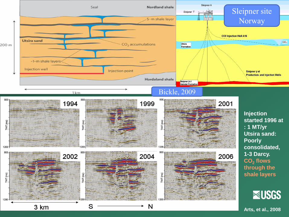
Arts, et al., 2008
Bickle, 2009
Injection
started 1996 at
: 1 MT/yr
Utsira sand:
Poorly
consolidated,
1-3 Darcy.
CO2 flows
through the
shale layers
Sleipner site
Norway
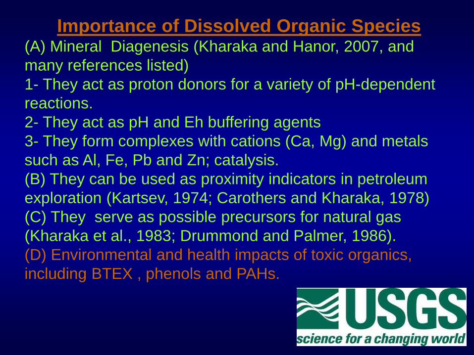
Importance of Dissolved Organic Species (A) Mineral Diagenesis (Kharaka and Hanor, 2007, and
many references listed)
1- They act as proton donors for a variety of pH-dependent
reactions.
2- They act as pH and Eh buffering agents
3- They form complexes with cations (Ca, Mg) and metals
such as Al, Fe, Pb and Zn; catalysis.
(B) They can be used as proximity indicators in petroleum
exploration (Kartsev, 1974; Carothers and Kharaka, 1978)
(C) They serve as possible precursors for natural gas
(Kharaka et al., 1983; Drummond and Palmer, 1986).
(D) Environmental and health impacts of toxic organics,
including BTEX , phenols and PAHs.
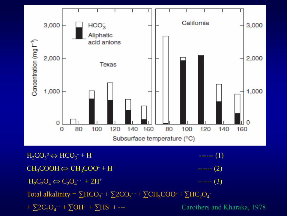
H2CO3o HCO3
- + H+ ------ (1)
CH3COOH CH3COO- + H+ ------ (2)
H2C2O4 C2O4- - + 2H+ ------ (3)
Total alkalinity = ∑HCO3- + ∑2CO3
- - + ∑CH3COO- + ∑HC2O4-
+ ∑2C2O4- - + ∑OH- + ∑HS- + --- Carothers and Kharaka, 1978
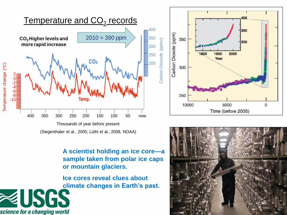
Temperature and CO2 records
400 350 300 250 200 150 100 50 now
Thousands of year before present
(Siegenthaler et al., 2005; Lüthi et al., 2008, NOAA)
20
-2-4-6-8
-10
Tem
pera
ture
change (
oC
)
400
350
300
250
200
Carb
on D
ioxode (
ppm
v)2010 = 390 ppmCO2 Higher levels and
more rapid increase
A scientist holding an ice core—a
sample taken from polar ice caps
or mountain glaciers.
Ice cores reveal clues about
climate changes in Earth’s past.
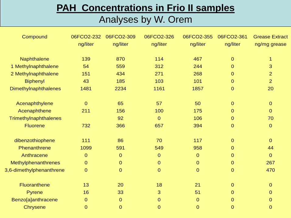
Compound 06FCO2-232 06FCO2-309 06FCO2-326 06FCO2-355 06FCO2-361 Grease Extract
ng/liter ng/liter ng/liter ng/liter ng/liter ng/mg grease
Naphthalene 139 870 114 467 0 1
1 Methylnaphthalene 54 559 312 244 0 3
2 Methylnaphthalene 151 434 271 268 0 2
Biphenyl 43 185 103 101 0 2
Dimethylnaphthalenes 1481 2234 1161 1857 0 20
Acenaphthylene 0 65 57 50 0 0
Acenaphthene 211 156 100 175 0 0
Trimethylnaphthalenes 92 0 106 0 70
Fluorene 732 366 657 394 0 0
dibenzothiophene 111 86 70 117 0 0
Phenanthrene 1099 591 549 958 0 44
Anthracene 0 0 0 0 0 0
Methylphenanthrenes 0 0 0 0 0 267
3,6-dimethylphenanthrene 0 0 0 0 0 470
Fluoranthene 13 20 18 21 0 0
Pyrene 16 33 3 51 0 0
Benzo[a]anthracene 0 0 0 0 0 0
Chrysene 0 0 0 0 0 0
PAH Concentrations in Frio II samples
Analyses by W. Orem
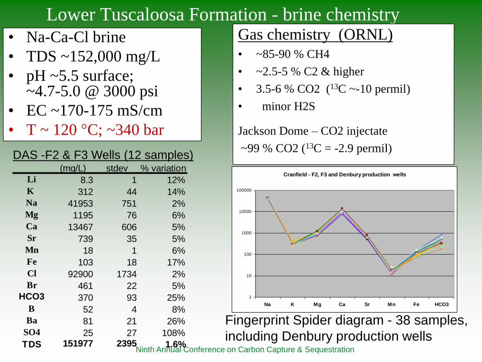
Ninth Annual Conference on Carbon Capture & Sequestration
• Na-Ca-Cl brine
• TDS ~152,000 mg/L
• pH ~5.5 surface; ~4.7-5.0 @ 3000 psi
• EC ~170-175 mS/cm
• T ~ 120 °C; ~340 bar
Fingerprint Spider diagram - 38 samples,
including Denbury production wells
DAS -F2 & F3 Wells (12 samples)
Cranfield - F2, F3 and Denbury production wells
1
10
100
1000
10000
100000
Na K Mg Ca Sr Mn Fe HCO3
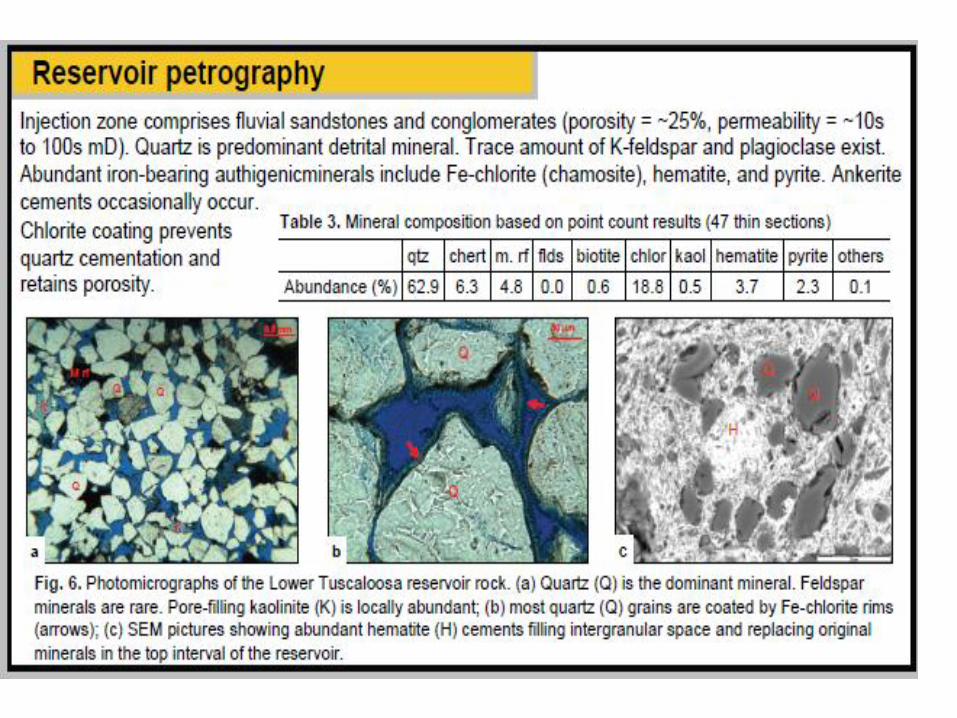
Lower Tuscaloosa Formation - brine chemistry
(mg/L) stdev % variation
Li 8.3 1 12%
K 312 44 14%
Na 41953 751 2%
Mg 1195 76 6%
Ca 13467 606 5%
Sr 739 35 5%
Mn 18 1 6%
Fe 103 18 17%
Cl 92900 1734 2%
Br 461 22 5%HCO3 370 93 25%
B 52 4 8%
Ba 81 21 26%
SO4 25 27 108%
TDS 151977 2395 1.6%
Gas chemistry (ORNL)
• ~85-90 % CH4
• ~2.5-5 % C2 & higher
• 3.5-6 % CO2 (13C ~-10 permil)
• minor H2S
Jackson Dome – CO2 injectate
~99 % CO2 (13C = -2.9 permil)

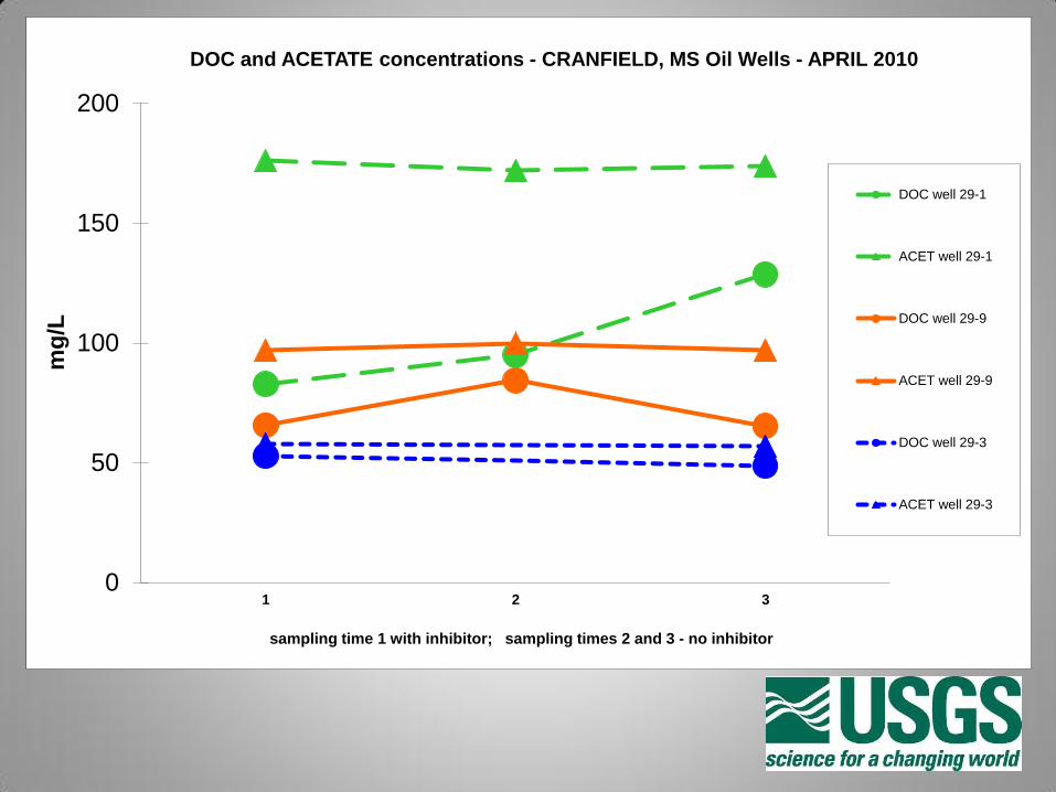
0
50
100
150
200
1 2 3
mg
/L
sampling time 1 with inhibitor; sampling times 2 and 3 - no inhibitor
DOC and ACETATE concentrations - CRANFIELD, MS Oil Wells - APRIL 2010
DOC well 29-1
ACET well 29-1
DOC well 29-9
ACET well 29-9
DOC well 29-3
ACET well 29-3

Impacts in the Pacific Coastline
California Wine Industry: Unwelcome Changes?
• Climate change affects managed ecosystems like vineyards and
farms just as it affects natural ecosystems
• Future warming unlikely to help wine growers in California’s
premium wine regions: some areas projected to become ―marginal‖
by 2100
National Academy of Sciences
National Academy of Engineering
Institute of Medicine
National Research Council
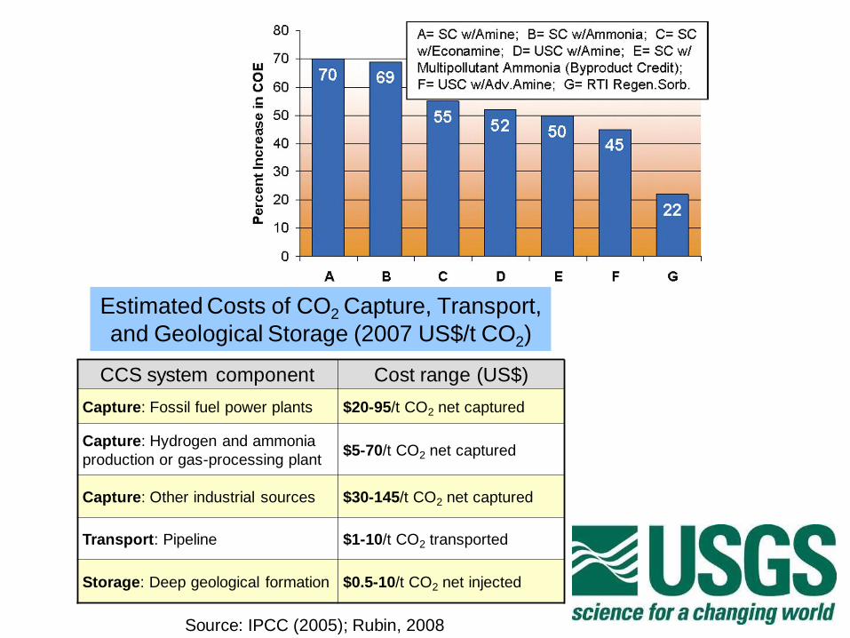
Estimated Costs of CO2 Capture, Transport,
and Geological Storage (2007 US$/t CO2)
CCS system component Cost range (US$)
Capture: Fossil fuel power plants $20-95/t CO2 net captured
Capture: Hydrogen and ammonia
production or gas-processing plant$5-70/t CO2 net captured
Capture: Other industrial sources $30-145/t CO2 net captured
Transport: Pipeline $1-10/t CO2 transported
Storage: Deep geological formation $0.5-10/t CO2 net injected
Source: IPCC (2005); Rubin, 2008
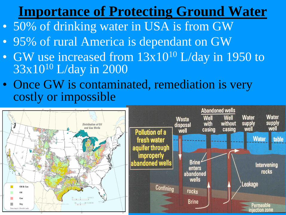
• 50% of drinking water in USA is from GW
• 95% of rural America is dependant on GW
• GW use increased from 13x1010 L/day in 1950 to 33x1010 L/day in 2000
• Once GW is contaminated, remediation is very costly or impossible
Importance of Protecting Ground Water
0
50
100
150
200
1 2 3
mg
/L
sampling time 1 with inhibitor; sampling times 2 and 3 - no inhibitor
DOC and ACETATE concentrations - CRANFIELD, MS Oil Wells - APRIL 2010
DOC well 29-1
ACET well 29-1
DOC well 29-9
ACET well 29-9
DOC well 29-3
ACET well 29-3
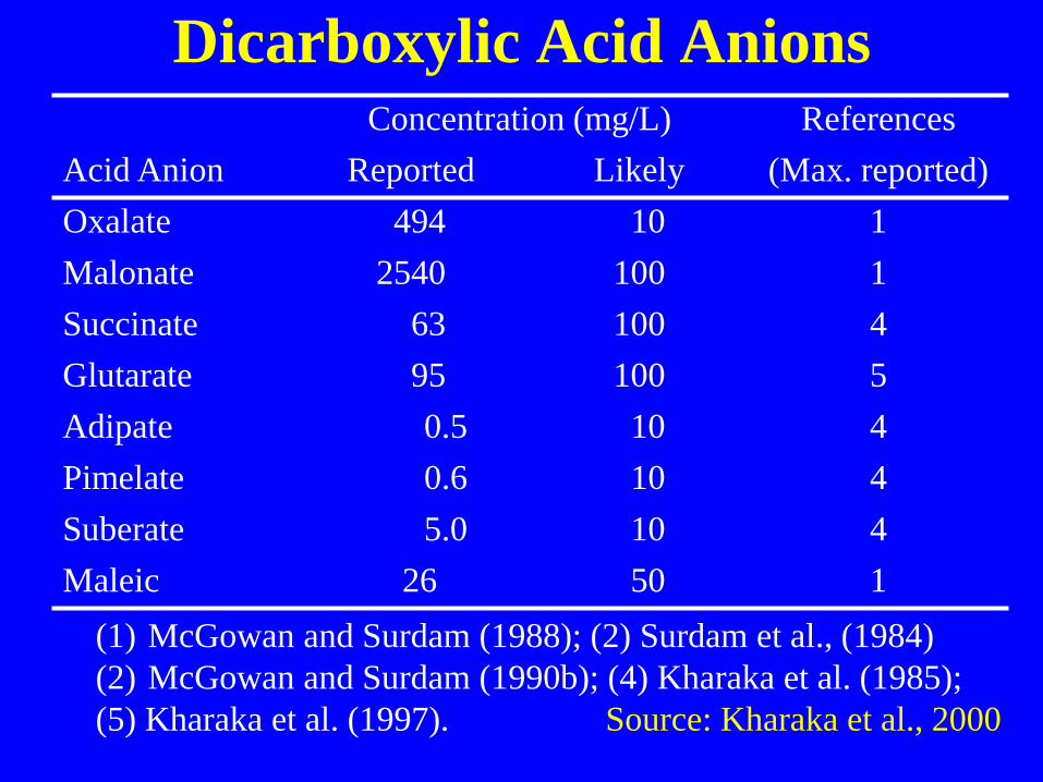
Concentration (mg/L) References
Acid Anion Reported Likely (Max. reported)
Oxalate 494 10 1
Malonate 2540 100 1
Succinate 63 100 4
Glutarate 95 100 5
Adipate 0.5 10 4
Pimelate 0.6 10 4
Suberate 5.0 10 4
Maleic 26 50 1
(1) McGowan and Surdam (1988); (2) Surdam et al., (1984)
(2) McGowan and Surdam (1990b); (4) Kharaka et al. (1985);
(5) Kharaka et al. (1997). Source: Kharaka et al., 2000
Dicarboxylic Acid Anions
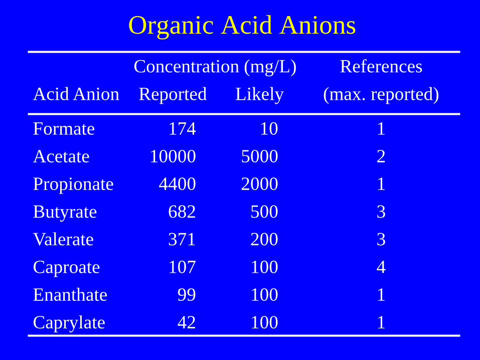
Concentration (mg/L) References
Acid Anion Reported Likely (max. reported)
Formate 174 10 1
Acetate 10000 5000 2
Propionate 4400 2000 1
Butyrate 682 500 3
Valerate 371 200 3
Caproate 107 100 4
Enanthate 99 100 1
Caprylate 42 100 1
Organic Acid Anions

Concentrations of DOC in Frio I brine
Frio I
1
10
100
1000
7/1/04 10/9/04 1/17/05 4/27/05 8/5/05 11/13/05 2/21/06
Date
DO
C (
mg
/L)
IW - pre CO2
OW - pre CO2
OW U-tube(10/5-10/7/04)-pre BT
OW U-tube(10/5-10/7/04)-post BT
OW U-tube(10/29-11/3/04)
IW post CO2 (4/4-4/5/05)
OW "B" post CO2 (4/5-4/6/05)
Kuster
IW (1/06)
OW "B" (1/06)
?
0.00
1.00
2.00
3.00
4.00
5.00
6.00
7.00
8.00
9.00
10.00
0 500 1000 1500 2000 2500 3000 3500
HCO3
DO
C
OW-pre
IW-pre
slugtest
OW-pre BT
OW-post BT
OW-10/9
OW-K 10/9/06
OW-11/2/06
IW-U
IW-K
Frio II
Organics in Oil-Field Water
(mg/L)
Frio DOC (6/04-4/05)
0
1
10
100
1000
Jun-04 Aug-04 Oct-04 Dec-04 Feb-05 Apr-05
DO
C (
mg
/L)
DOC injection w ell
DOC observation w ell C-sand
DOC observation w ell B-sand
Organics in Produced Water
(mg/L)
0.7Ground Water
7Surface Water
5-1000Produced Water
MeanDOC
0.7Ground Water
7Surface Water
5-1000Produced Water
MeanDOC
Kharaka & Hanor, 2004
1.23 – HYDROXY BENZOIC ACID
0.22 – HYROXY BENZOIC ACID
44 – METHYL BENZOIC ACID
5BENZOIC ACID
24 – METHYL PHENOL
10,000
60
10
20
ACETATE & OTHER ACID
ANIONS
BTEX
PAHs
PHENOL
Kharaka & Hanor, 2004
1.23 – HYDROXY BENZOIC ACID
0.22 – HYROXY BENZOIC ACID
44 – METHYL BENZOIC ACID
5BENZOIC ACID
24 – METHYL PHENOL
10,000
60
10
20
ACETATE & OTHER ACID
ANIONS
BTEX
PAHs
PHENOL
Kharaka & Hanor, 2007 Classes & Importance of Dissolved Organic Species
(1) Hydrocarbons; (2) Organic acid anions; & (3) Toxic Organics
(2-A) Mineral Diagenesis (Kharaka and Hanor, 2007, and many references listed)
1- They act as proton donors for a variety of pH-dependent reactions.
2- They act as pH and Eh buffering agents
3- They form complexes with cations (Ca, Mg) and metals such as Al, Fe, Pb and Zn; catalysis.
(3-A) High environmental and health impacts of toxic organics, especially BTEX , phenols and PAHs.
1- May be present in brines at 10s of mg/L
2- High toxicity--MCL at low ppb levels
2- Partition into & potential to leak with the super critical CO2 into GW .
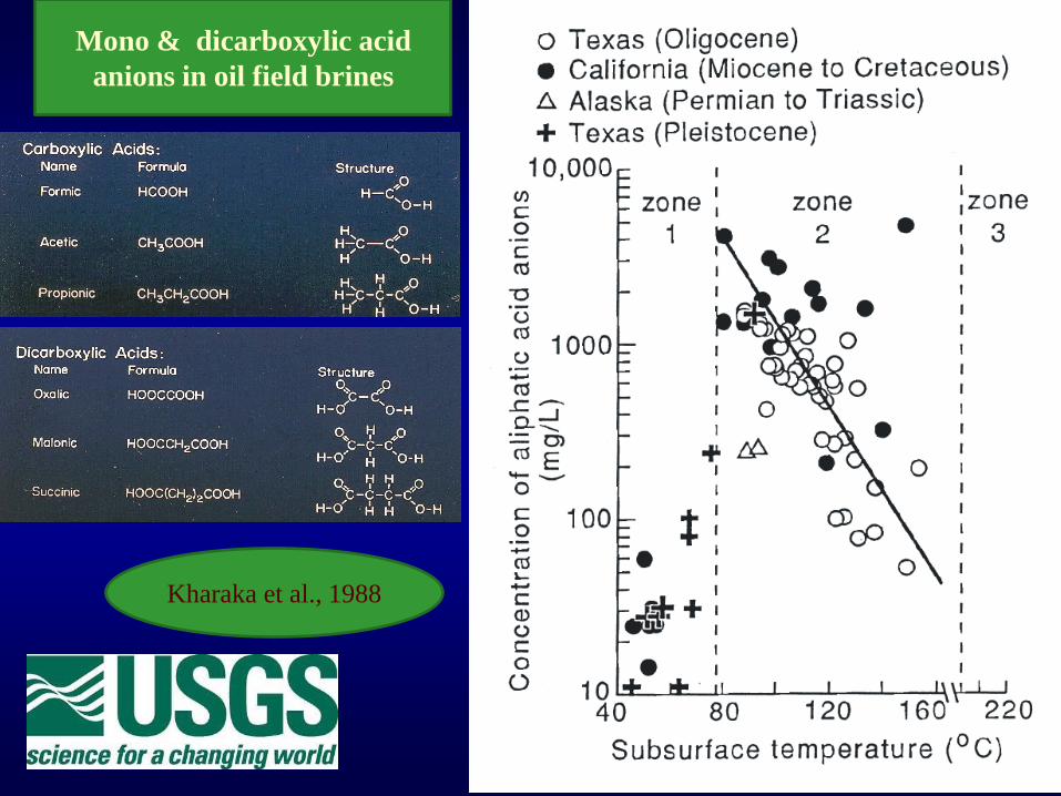
Mono & dicarboxylic acid
anions in oil field brines
Kharaka et al., 1988