Embed Size (px)
Citation preview
1
KAUSHIK BASU*
World Bank
BARRY EICHENGREEN†
University of California, Berkeley
POONAM GUPTA‡
World Bank
From Tapering to Tightening: The Impact of the Fed’s Exit on India§
ABSTRACT The episode of volatility starting on May 22, 2013, when Federal Reserve Chairman Ben Bernanke first spoke of the possibility of the US central bank “tapering” its security purchases, had a sharp negative impact on emerging markets. India was among those hardest hit. The rupee depreciated by 18 percent at one point, causing concerns that the country was heading toward a financial crisis. This paper contends that India was adversely impacted because it had received large capital flows in prior years and had large and liquid financial markets that were a convenient target for investors seeking to rebalance away from emerging markets. In addition, macroeconomic conditions had weakened in prior years, which rendered the economy vulnerable to capital outflows and limited the policy room for maneuver. Measures adopted to handle the impact of the tapering talk were not effective in stabilizing the financial markets and restoring confidence, implying that there may not be any easy choices when a country is caught in the midst of rebalancing of global portfolios. We suggest putting in place a medium-term policy framework that limits vulnerabilities in advance, while maximizing the policy space for responding to shocks. Elements of such a framework include a sound fiscal bal-ance, sustainable current account deficit, and environment conducive to investment. In addition, India should continue to encourage stable longer term capital inflows while discouraging volatile short-term flows, hold a larger stock of reserves, avoid excessive appreciation of the exchange rate through interventions with the use of reserves and macroprudential policy, and prepare the banks and firms to handle greater exchange rate volatility.
* [email protected]† [email protected]‡ [email protected]§ We thank Shankar Acharya, Rahul Anand, Paul Cashin, Tito Cordella, Subir Gokarn,
Manoj Govil, Muneesh Kapur, Kenneth Kletzer, Rakesh Mohan, Zia Qureshi, Y.V. Reddy, David Rosenblatt, Aristomene Varoudakis, and participants of the India Policy Forum, 2014, for very useful discussions and comments, and Serhat Solmaz for excellent research assistance.
2 IND IA POL ICY FORUM, 2014–15
Keywords: Balance of Payments, Economic Management, Macroeconomic Policy, Macroeconomic Vulnerability, Monetary Policy
JEL Classification: F32, F33, F38, E58
1. Introduction
On May 22, 2013, Federal Reserve Chairman Ben Bernanke first spoke of the possibility of the Fed reducing, or tapering, its security
purchases. This “tapering talk,” as it came to be known, had a sharp nega-tive impact on financial conditions in emerging markets.1 India was among those hardest hit. Between May 22, 2013, and the end of August 2013, the rupee depreciated by 18 percent, bond spreads increased, and equity prices fell. The reaction was sufficiently pronounced for the press to warn that India might be heading toward a full-blown financial crisis, requiring the country to seek IMF assistance.2
In this paper, we ask three questions about this episode. Why was the impact of the Fed’s announcement on India so severe? How effective were the policy measures undertaken in response? How can India prepare itself for the normalization of monetary policy in advanced economies and more broadly to react to global liquidity cycles?
Eichengreen and Gupta (2014) analyzed the impact of the Fed’s taper-ing talk on exchange rates, foreign reserves, and equity prices in emerging markets between April and August 2013.3 They established that an important determinant of the impact was the volume of capital flows that countries received in prior years and the size of local financial markets. Countries receiving larger inflows of capital and with larger and liquid financial markets experienced more pressure on their exchange rates, reserves, and equity prices once the Fed’s “tapering talk” began. This may be interpreted as showing that investors are better able to rebalance their portfolios away
1. The period of the tapering talk is generally referred to that between May 22, 2013 and September 18, 2013.
2. See e.g., “India in crisis mode as rupee hits another record low,” http://money.cnn.com/2013/08/28/investing/india-rupee/ (Accessed April 30, 2015); “India’s Financial Crisis, Through the Keyhole,” http://www.economist.com/blogs/banyan/2013/08/india-s-financial-crisis (Accessed April 30, 2015).
3. Subsequently the Federal Reserve started tapering its purchases of securities in December 2013, reducing it by $10 bn each month. It has since then tapered six more times, each time by $10 bn and is expected to end the program in October, 2014, with a last reduction of $15 bn in the purchase of securities.
Kaushik Basu et al. 3
from an emerging economy when the country in question has a relatively large and liquid financial market.
This paper elaborates the Indian case. India ranks high in terms of the size and liquidity of its financial markets and the extent of capital flows it received in prior years. It thus was an easy target for investors seeking to rebalance away from emerging markets.
In addition, Eichengreen and Gupta show that the emerging markets that allowed their real exchange rates to appreciate and their current account deficits to widen in the period of quantitative easing felt a larger impact. Such vulnerabilities had developed in India too in prior years. In addition, the country’s fiscal deficit had increased, and inflation at about 10 percent was stubbornly high. These macroeconomic weaknesses had surfaced in the midst of a sharp growth slowdown. Although the level of foreign reserves was considered comfortable by some metrics, effective coverage had declined since 2008.
The specific factors contributing to the high fiscal or current account defi-cit in India also indicated increased economic and financial vulnerabilities. The increase in fiscal deficit was due to an increase in current expenditure (in response to the global financial crisis of 2008, the headwinds of which were palpable by early 2009), rather than to a pick up in public investment. The increase in current account deficit, largely a mirror image of the increased current expenditure, was characterized by the diversion of private savings into the import of gold. It reflected a dearth of attractive domestic outlets for personal savings in a high inflation environment, where real returns on many domestic financial investments had turned negative. Loose monetary policy in the advanced countries made those deficits easy to finance, further reliev-ing the pressure to compress them. Rebalancing by global investors when the Fed broached the subject of tapering highlighted these vulnerabilities.
The authorities adopted a range of measures in response. They intervened in the foreign exchange market, hiked interest rates, raised the import duty on gold, encouraged capital inflows from nonresident Indians, established a currency swap window for oil importing companies, opened a swap line with the Bank of Japan, and restricted capital outflows from residents and Indian companies. We estimate the impact of these measures on the exchange rate and financial markets. Our results show that some of these measures, includ-ing the separate swap window for oil importing companies, were of limited help in stabilizing the financial markets. Others, like initiatives restricting capital outflows, actually undermined confidence.
These findings imply that there are no easy choices when a country is affected by a rebalancing of global portfolios. Hence, we suggest putting in
4 IND IA POL ICY FORUM, 2014–15
place a medium-term policy framework that limits vulnerabilities in advance, while maximizing the policy space for responding to shocks. Elements of such a framework include holding a larger stock of reserves; avoiding exces-sive appreciation of the exchange rate through interventions using reserves and macroprudential policy; signing swap lines with other central banks where feasible; preparing the banks and the corporates to handle greater exchange rate volatility; adopting a clear communication strategy; avoiding measures that could damage confidence, such as restricting outflows; and managing capital inflows to encourage relatively stable longer term flows while discouraging short-term flows.4 A sound fiscal balance, sustainable current account deficit, and environment conducive for investment are other obvious elements of this policy framework.
2. The Effects of the Tapering Talk on India
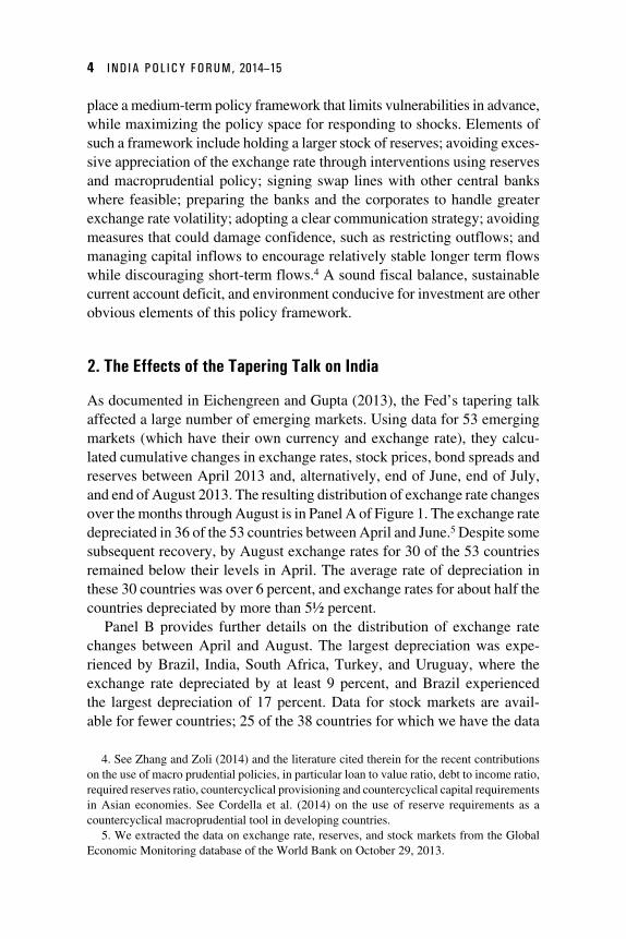
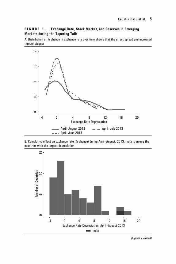
As documented in Eichengreen and Gupta (2013), the Fed’s tapering talk affected a large number of emerging markets. Using data for 53 emerging markets (which have their own currency and exchange rate), they calcu-lated cumulative changes in exchange rates, stock prices, bond spreads and reserves between April 2013 and, alternatively, end of June, end of July, and end of August 2013. The resulting distribution of exchange rate changes over the months through August is in Panel A of Figure 1. The exchange rate depreciated in 36 of the 53 countries between April and June.5 Despite some subsequent recovery, by August exchange rates for 30 of the 53 countries remained below their levels in April. The average rate of depreciation in these 30 countries was over 6 percent, and exchange rates for about half the countries depreciated by more than 5½ percent.
Panel B provides further details on the distribution of exchange rate changes between April and August. The largest depreciation was expe-rienced by Brazil, India, South Africa, Turkey, and Uruguay, where the exchange rate depreciated by at least 9 percent, and Brazil experienced the largest depreciation of 17 percent. Data for stock markets are avail-able for fewer countries; 25 of the 38 countries for which we have the data
4. See Zhang and Zoli (2014) and the literature cited therein for the recent contributions on the use of macro prudential policies, in particular loan to value ratio, debt to income ratio, required reserves ratio, countercyclical provisioning and countercyclical capital requirements in Asian economies. See Cordella et al. (2014) on the use of reserve requirements as a countercyclical macroprudential tool in developing countries.
5. We extracted the data on exchange rate, reserves, and stock markets from the Global Economic Monitoring database of the World Bank on October 29, 2013.
Kaushik Basu et al. 5
F I G U R E 1 . Exchange Rate, Stock Market, and Reserves in Emerging Markets during the Tapering TalkA: Distribution of % change in exchange rate over time shows that the effect spread and increased through August
0 .0
5 .1
.1
5 .2
–4 0 4 8 12 16 20Exchange Rate Depreciation
April–August 2013 April–July 2013 April–June 2013
B: Cumulative effect on exchange rate (% change) during April–August, 2013, India is among the countries with the largest depreciation
–4 0 4 8 12 16 20
0 5
10
15
Exchange Rate Depreciation, April–August 2013
Num
ber o
f Cou
ntrie
s
India
(Figure 1 Contd)
6 IND IA POL ICY FORUM, 2014–15
C: Cumulative effect on stock market index (% change) between April–August, 2013 is rather modest for India
India
–30 –25 –20 –15 –10 –5 0 5 10 15 20 25 30
0 2
4 6
8 10
% Change in Stock Market April–August 2013
Num
ber o
f Cou
ntrie
s
D: Cumulative effect on external reserves (% change) during April–August, 2013, reserves declined by nearly 6% in India
India
–25 –20 –15 –10 –5 0 5 10 15 20
0 5
10
15
% Change in Reserves April–August 2013
Num
ber o
f Cou
ntrie
s
Source: Data on exchange rates, reserves and stock markets are from the Global Economic Monitoring database of the World Bank. Calculations are based on end of month values. See Eichengreen and Gupta (2014) for details.
(Figure 1 Contd)
Kaushik Basu et al. 7
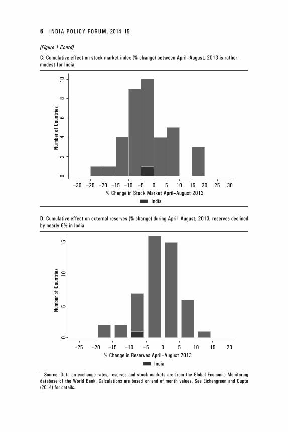
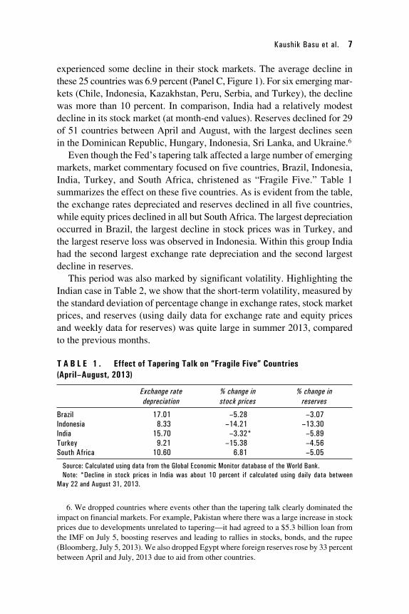
experienced some decline in their stock markets. The average decline in these 25 countries was 6.9 percent (Panel C, Figure 1). For six emerging mar-kets (Chile, Indonesia, Kazakhstan, Peru, Serbia, and Turkey), the decline was more than 10 percent. In comparison, India had a relatively modest decline in its stock market (at month-end values). Reserves declined for 29 of 51 countries between April and August, with the largest declines seen in the Dominican Republic, Hungary, Indonesia, Sri Lanka, and Ukraine.6
Even though the Fed’s tapering talk affected a large number of emerging markets, market commentary focused on five countries, Brazil, Indonesia, India, Turkey, and South Africa, christened as “Fragile Five.” Table 1 summarizes the effect on these five countries. As is evident from the table, the exchange rates depreciated and reserves declined in all five countries, while equity prices declined in all but South Africa. The largest depreciation occurred in Brazil, the largest decline in stock prices was in Turkey, and the largest reserve loss was observed in Indonesia. Within this group India had the second largest exchange rate depreciation and the second largest decline in reserves.
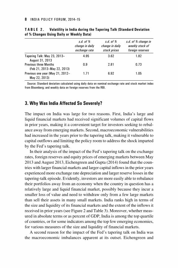
This period was also marked by significant volatility. Highlighting the Indian case in Table 2, we show that the short-term volatility, measured by the standard deviation of percentage change in exchange rates, stock market prices, and reserves (using daily data for exchange rate and equity prices and weekly data for reserves) was quite large in summer 2013, compared to the previous months.
T A B L E 1 . Effect of Tapering Talk on “Fragile Five” Countries (April–August, 2013)
Exchange rate depreciation
% change in stock prices
% change in reserves
Brazil 17.01 –5.28 –3.07Indonesia 8.33 –14.21 –13.30India 15.70 –3.32* –5.89Turkey 9.21 –15.38 –4.56South Africa 10.60 6.81 –5.05
Source: Calculated using data from the Global Economic Monitor database of the World Bank.Note: *Decline in stock prices in India was about 10 percent if calculated using daily data between
May 22 and August 31, 2013.
6. We dropped countries where events other than the tapering talk clearly dominated the impact on financial markets. For example, Pakistan where there was a large increase in stock prices due to developments unrelated to tapering—it had agreed to a $5.3 billion loan from the IMF on July 5, boosting reserves and leading to rallies in stocks, bonds, and the rupee (Bloomberg, July 5, 2013). We also dropped Egypt where foreign reserves rose by 33 percent between April and July, 2013 due to aid from other countries.
8 IND IA POL ICY FORUM, 2014–15
3. Why Was India Affected So Severely?
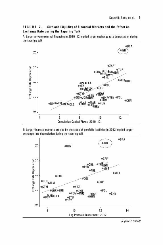
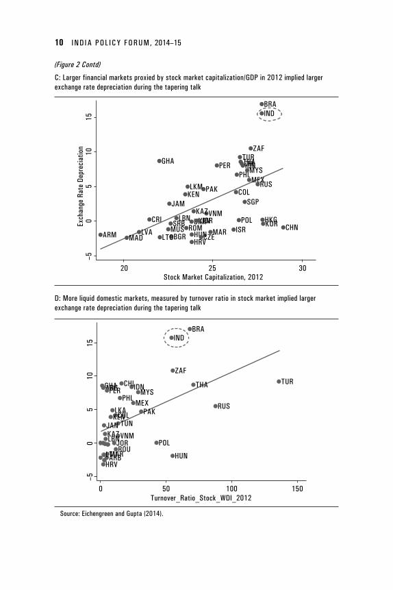
The impact on India was large for two reasons. First, India’s large and liquid financial markets had received significant volumes of capital flows in prior years, making it a convenient target for investors seeking to rebal-ance away from emerging markets. Second, macroeconomic vulnerabilities had increased in the years prior to the tapering talk, making it vulnerable to capital outflows and limiting the policy room to address the shock imparted by the Fed’s tapering talk.
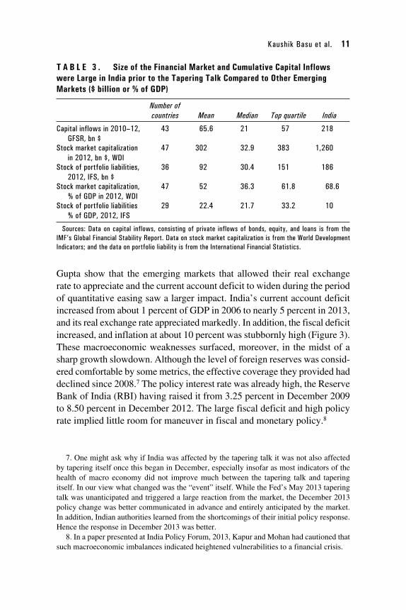
In their analysis of the impact of the Fed’s tapering talk on the exchange rates, foreign reserves and equity prices of emerging markets between May 2013 and August 2013, Eichengreen and Gupta (2014) found that the coun-tries with larger financial markets and larger capital inflows in the prior years experienced more exchange rate depreciation and larger reserve losses in the tapering-talk episode. Evidently, investors are more easily able to rebalance their portfolios away from an economy when the country in question has a relatively large and liquid financial market, possibly because they incur a smaller loss of value and need to withdraw only from a few large markets than sell their assets in many small markets. India ranks high in terms of the size and liquidity of its financial markets and the extent of the inflows it received in prior years (see Figure 2 and Table 3). Moreover, whether meas-ured in absolute terms or as percent of GDP, India is among the top quartile of countries, or for some indicators among the top few emerging economies, for various measures of the size and liquidity of financial markets.
A second reason for the impact of the Fed’s tapering talk on India was the macroeconomic imbalances apparent at its outset. Eichengreen and
T A B L E 2 . Volatility in India during the Tapering Talk (Standard Deviation of % Changes Using Daily or Weekly Data)
s.d. of % change in daily exchange rate
s.d. of % change in daily
stock prices
s.d. of % change in weekly stock of foreign reserves
Tapering Talk: May 23, 2013–August 31, 2013
4.95 3.62 1.82
Previous three Months (Feb 21, 2013–May 22, 2013)
0.9 2.81 0.73
Previous one year (May 21, 2012–May 22, 2013)
1.71 6.92 1.05
Source: Standard deviation calculated using daily data on nominal exchange rate and stock market index from Bloomberg; and weekly data on foreign reserves from the RBI.
Kaushik Basu et al. 9
F I G U R E 2 . Size and Liquidity of Financial Markets and the Effect on Exchange Rate during the Tapering TalkA: Larger private external financing in 2010–12 implied larger exchange rate depreciation during the tapering talk
•LKA•KEN
•GTM
•ARM •DLB
•LBN•KAZ
•BLR
•VNM•SRB•AZE•CRI •JOR
•BGR•LVA•LTU•MAR
•HRV•HUN
•ROM
•NOM•JAM
•PHL•PER •CHL
•ZAF
•IND•BRA
•GHA•TUR
•IDN•MYS
•MEX•RUS
•CHN•POL
•COL
•THA
4 6 8 10 12Cumulative Capital Flows, 2010–12
Exch
ange
Rat
e De
prec
iatio
n
•VEN•UKR
•MKA•BIH
–5
0 5
10
15
•PAK
•TUD
B: Larger financial markets proxied by the stock of portfolio liabilities in 2012 implied larger exchange rate depreciation during the tapering talk
•PAK
•BLR•JAM•GTM
•PHL•PER
•CHL
•ZAF
•IND•BRA
•URY
•TUR•IDN•MYS
•MEX
•CHN•POL
•SGP
•ISR•HUN
•COL
•KAZ•UKR•MUS•ROM
•LTU•HRV
•BGRMAR•LVA
•JOR •SRB
•THA
8 10 12 14Log Portfolio Investment, 2012
Exch
ange
Rat
e De
prec
iatio
n–5
0
5 10
15
(Figure 2 Contd)
10 IND IA POL ICY FORUM, 2014–15
C: Larger financial markets proxied by stock market capitalization/GDP in 2012 implied larger exchange rate depreciation during the tapering talk
•VNM
–5
0 5
10
15Ex
chan
ge R
ate
Depr
ecia
tion
20 25 30
•JAM
•PHL•PER •CHL
•ZAF
•IND•BRA
•TUR•IDN
•MYS•MEX•RUS
•CHN•HKG•KOR•POL
•SGP
•ISR•HUN
•COL
•KAZ•LBN
•SRB•MUS•BGR •CZE
•ROM•UKR•VEN•JOR
•HRV•ARM •MAD
•LVA
•CRI
•GHA
•PAK•LKM•KEN
•MAR
•THA
Stock Market Capitalization, 2012
•LTO
D: More liquid domestic markets, measured by turnover ratio in stock market implied larger exchange rate depreciation during the tapering talk
–5
0 5
10
15
0 50 100 150Turnover_Ratio_Stock_WDI_2012
•TUR
•BRA•IND
•ZAF
•THA
•RUS
•POL
•HUN
•PAK•MEX
•MYS•IDN•CHL•GHA•ARG•PER
•PHL
•LKA•COL•KEN•TUN•JAN
•KAZ•VNM•LBN•JOR•ROU
•MAR•HRV•ARBLTU
Source: Eichengreen and Gupta (2014).
(Figure 2 Contd)
Kaushik Basu et al. 11
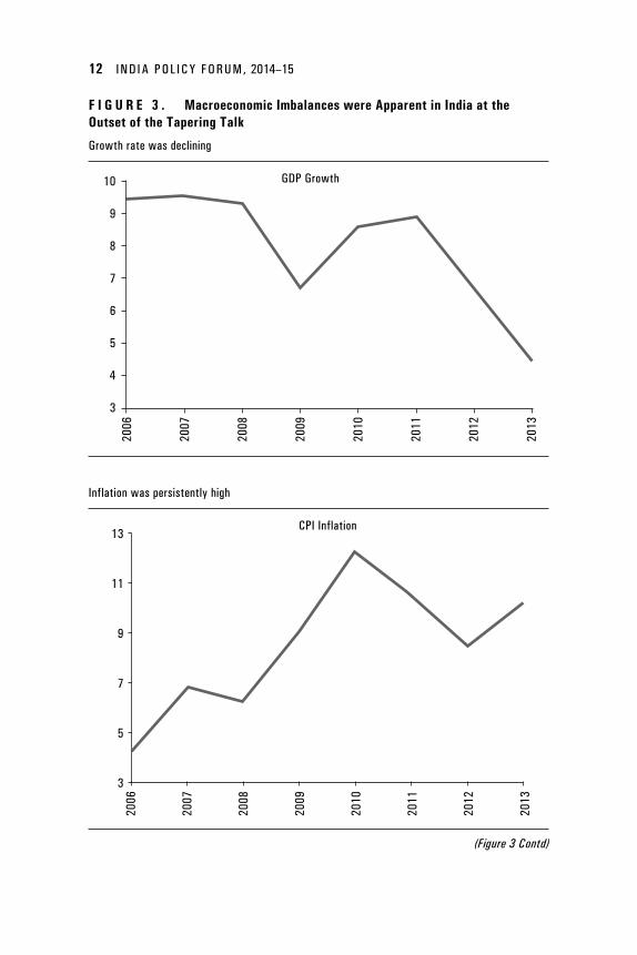
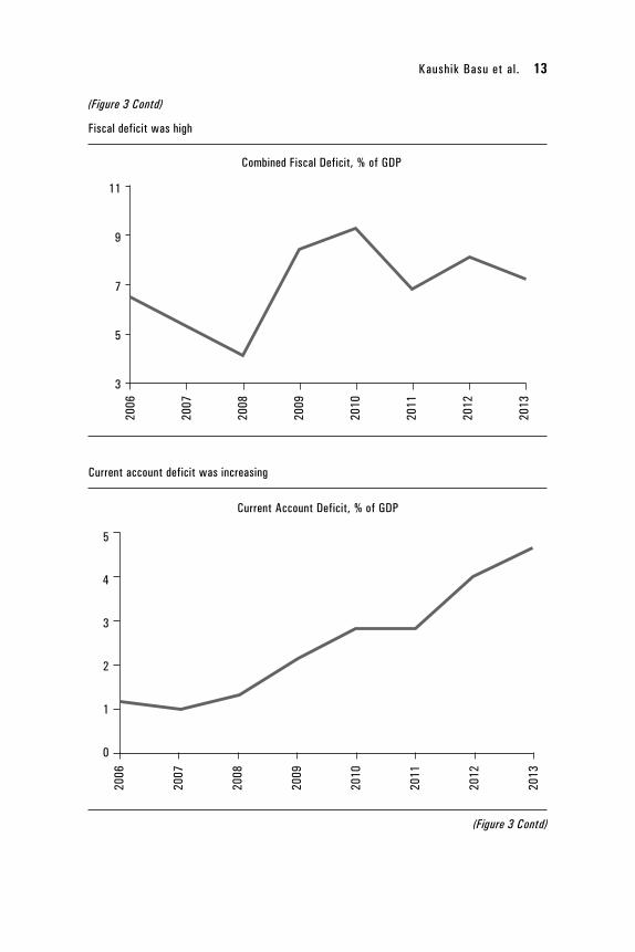
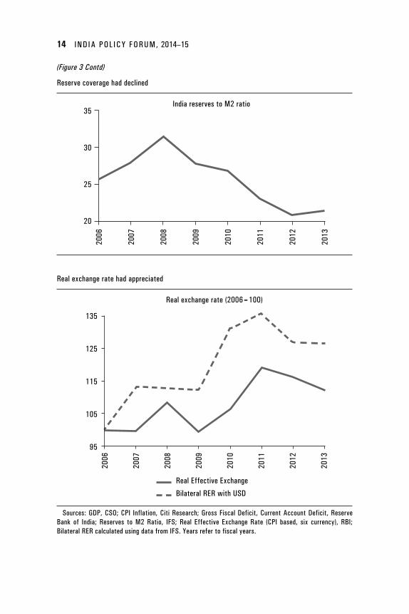
Gupta show that the emerging markets that allowed their real exchange rate to appreciate and the current account deficit to widen during the period of quantitative easing saw a larger impact. India’s current account deficit increased from about 1 percent of GDP in 2006 to nearly 5 percent in 2013, and its real exchange rate appreciated markedly. In addition, the fiscal deficit increased, and inflation at about 10 percent was stubbornly high (Figure 3). These macroeconomic weaknesses surfaced, moreover, in the midst of a sharp growth slowdown. Although the level of foreign reserves was consid-ered comfortable by some metrics, the effective coverage they provided had declined since 2008.7 The policy interest rate was already high, the Reserve Bank of India (RBI) having raised it from 3.25 percent in December 2009 to 8.50 percent in December 2012. The large fiscal deficit and high policy rate implied little room for maneuver in fiscal and monetary policy.8
7. One might ask why if India was affected by the tapering talk it was not also affected by tapering itself once this began in December, especially insofar as most indicators of the health of macro economy did not improve much between the tapering talk and tapering itself. In our view what changed was the “event” itself. While the Fed’s May 2013 tapering talk was unanticipated and triggered a large reaction from the market, the December 2013 policy change was better communicated in advance and entirely anticipated by the market. In addition, Indian authorities learned from the shortcomings of their initial policy response. Hence the response in December 2013 was better.
8. In a paper presented at India Policy Forum, 2013, Kapur and Mohan had cautioned that such macroeconomic imbalances indicated heightened vulnerabilities to a financial crisis.
T A B L E 3 . Size of the Financial Market and Cumulative Capital Inflows were Large in India prior to the Tapering Talk Compared to Other Emerging Markets ($ billion or % of GDP)
Number of countries Mean Median Top quartile India
Capital inflows in 2010–12, GFSR, bn $
43 65.6 21 57 218
Stock market capitalization in 2012, bn $, WDI
47 302 32.9 383 1,260
Stock of portfolio liabilities, 2012, IFS, bn $
36 92 30.4 151 186
Stock market capitalization, % of GDP in 2012, WDI
47 52 36.3 61.8 68.6
Stock of portfolio liabilities % of GDP, 2012, IFS
29 22.4 21.7 33.2 10
Sources: Data on capital inflows, consisting of private inflows of bonds, equity, and loans is from the IMF’s Global Financial Stability Report. Data on stock market capitalization is from the World Development Indicators; and the data on portfolio liability is from the International Financial Statistics.
12 IND IA POL ICY FORUM, 2014–15
F I G U R E 3 . Macroeconomic Imbalances were Apparent in India at the Outset of the Tapering Talk
Growth rate was declining
10
9
8
7
6
5
4
3
GDP Growth
2006
2007
2008
2009
2010
2011
2012
2013
Inflation was persistently high
CPI Inflation13
11
9
7
5
3
2006
2007
2008
2009
2010
2011
2012
2013
(Figure 3 Contd)
Kaushik Basu et al. 13
(Figure 3 Contd)
Fiscal deficit was high20
06
2007
2008
2009
2010
2011
2012
2013
11
9
7
5
3
Combined Fiscal Deficit, % of GDP
Current account deficit was increasing
Current Account Deficit, % of GDP
5
4
3
2
1
0
2006
2007
2008
2009
2010
2011
2012
2013
(Figure 3 Contd)
14 IND IA POL ICY FORUM, 2014–15
(Figure 3 Contd)
Reserve coverage had declined
2006
2007
2008
2009
2010
2011
2012
2013
35
30
25
20
India reserves to M2 ratio
Real exchange rate had appreciated
Real Effective Exchange
Bilateral RER with USD
Real exchange rate (2006=100)
2006
2007
2008
2009
2010
2011
2012
2013
135
125
115
105
95
Sources: GDP, CSO; CPI Inflation, Citi Research; Gross Fiscal Deficit, Current Account Deficit, Reserve Bank of India; Reserves to M2 Ratio, IFS; Real Effective Exchange Rate (CPI based, six currency), RBI; Bilateral RER calculated using data from IFS. Years refer to fiscal years.
Kaushik Basu et al. 15
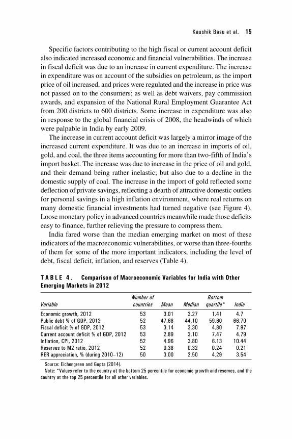
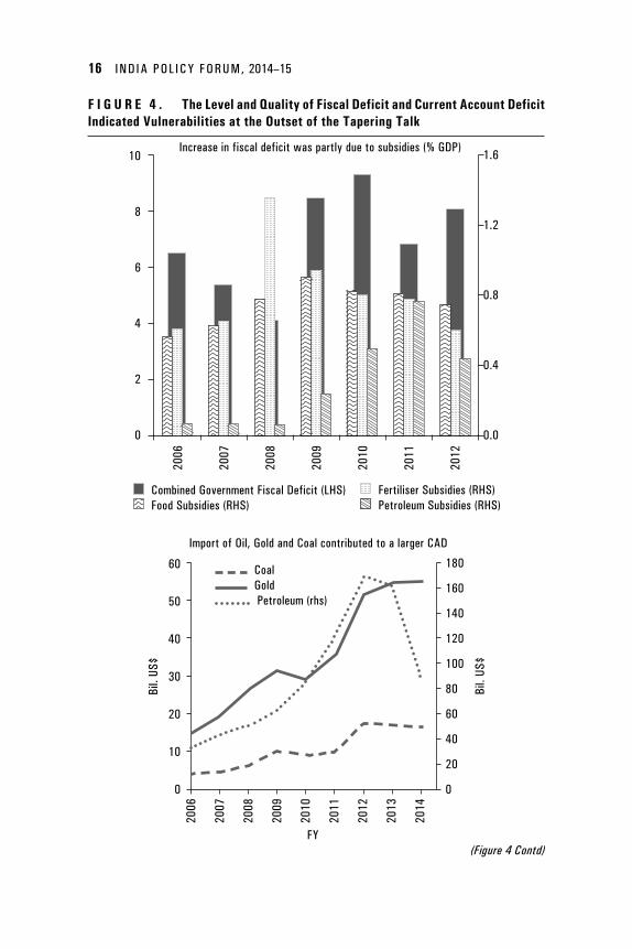
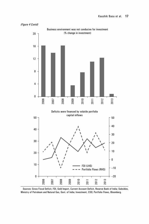
Specific factors contributing to the high fiscal or current account deficit also indicated increased economic and financial vulnerabilities. The increase in fiscal deficit was due to an increase in current expenditure. The increase in expenditure was on account of the subsidies on petroleum, as the import price of oil increased, and prices were regulated and the increase in price was not passed on to the consumers; as well as debt waivers, pay commission awards, and expansion of the National Rural Employment Guarantee Act from 200 districts to 600 districts. Some increase in expenditure was also in response to the global financial crisis of 2008, the headwinds of which were palpable in India by early 2009.
The increase in current account deficit was largely a mirror image of the increased current expenditure. It was due to an increase in imports of oil, gold, and coal, the three items accounting for more than two-fifth of India’s import basket. The increase was due to increase in the price of oil and gold, and their demand being rather inelastic; but also due to a decline in the domestic supply of coal. The increase in the import of gold reflected some deflection of private savings, reflecting a dearth of attractive domestic outlets for personal savings in a high inflation environment, where real returns on many domestic financial investments had turned negative (see Figure 4). Loose monetary policy in advanced countries meanwhile made those deficits easy to finance, further relieving the pressure to compress them.
India fared worse than the median emerging market on most of these indicators of the macroeconomic vulnerabilities, or worse than three-fourths of them for some of the more important indicators, including the level of debt, fiscal deficit, inflation, and reserves (Table 4).
T A B L E 4 . Comparison of Macroeconomic Variables for India with Other Emerging Markets in 2012
VariableNumber of countries Mean Median
Bottom quartile* India
Economic growth, 2012 53 3.01 3.27 1.41 4.7Public debt % of GDP, 2012 52 47.68 44.10 59.60 66.70Fiscal deficit % of GDP, 2012 53 3.14 3.30 4.80 7.97Current account deficit % of GDP, 2012 53 2.89 3.10 7.47 4.79Inflation, CPI, 2012 52 4.96 3.80 6.13 10.44Reserves to M2 ratio, 2012 52 0.38 0.32 0.24 0.21RER appreciation, % (during 2010–12) 50 3.00 2.50 4.29 3.54
Source: Eichengreen and Gupta (2014).Note: *Values refer to the country at the bottom 25 percentile for economic growth and reserves, and the
country at the top 25 percentile for all other variables.
16 IND IA POL ICY FORUM, 2014–15
F I G U R E 4 . The Level and Quality of Fiscal Deficit and Current Account Deficit Indicated Vulnerabilities at the Outset of the Tapering Talk
1.6
1.2
0.8
0.4
0.0
2006
2007
2008
2009
2010
2011
2012
10
8
6
4
2
0
Increase in fiscal deficit was partly due to subsidies (% GDP)
Combined Government Fiscal Deficit (LHS) Food Subsidies (RHS)
Fertiliser Subsidies (RHS) Petroleum Subsidies (RHS)
60
50
40
30
20
10
0
180
160
140
120
100
80
60
40
20
0
2006
2007
2008
2009
2010
2011
2012
2013
2014
Coal Gold Petroleum (rhs)
Import of Oil, Gold and Coal contributed to a larger CAD
Bil.
US$
Bil.
US$
FY(Figure 4 Contd)
Kaushik Basu et al. 17
(Figure 4 Contd)
2006
2007
2008
2009
2010
2011
2012
2013
20
16
12
8
4
0
Business environment was not conducive for investment (% change in investment)
50
40
30
20
10
0
–10
–20
50
40
30
20
10
0
2006
2007
2008
2009
2010
2011
2012
2013
FDI (LHS) Portfolio Flows (RHS)
Deficits were financed by volatile portfolio capital inflows
Sources: Gross Fiscal Deficit, FDI, Gold Import, Current Account Deficit, Reserve Bank of India; Subsidies, Ministry of Petroleum and Natural Gas, Govt. of India; Investment, CSO; Portfolio Flows, Bloomberg.
18 IND IA POL ICY FORUM, 2014–15
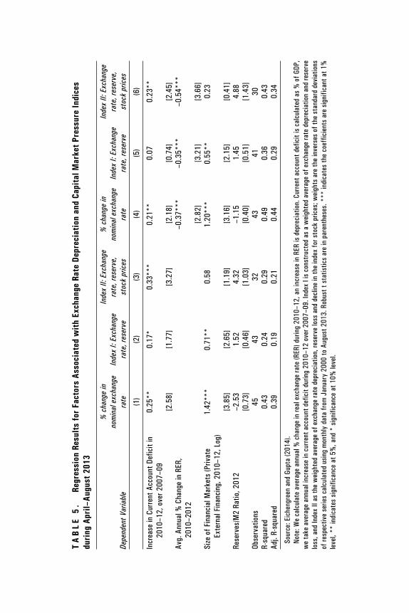
Drawing on Eichengreen and Gupta (2014), we consider the factors that were associated with the impact of the Fed’s tapering talk on exchange rates, stock prices, and reserves. We calculate weighted average of changes in exchange rates, foreign reserves, and stock prices in two separate indices. Capital Market Pressure Index I is a weighted average of percent deprecia-tion of exchange rate and reserves losses between April 2013 and August 2013, where the weights are the inverse of the standard deviations of monthly data from January 2000 to August 2013.
Capital Market Pressure Index I
=
% Exchange Rate Depreciation
+
% Decline in Reserves
σ exchange rate σ reserves
Capital Market Pressure Index II is similarly a weighted average of the percent depreciation of exchange rate, reserve loss, and decline in stock prices between April 2013 and August 2013.9
Capital Market Pressure Index II
=
% Exchange Rate Depreciation
+
% Decline in Reserves +
% Decline in Stock Market
σ exchange rate σ reserves σ stock
We regress exchange rate depreciation, Index I, and Index II on macroeco-nomic conditions, financial market structure and institutional variables, estimating linear equations of the form:
Yi = αk Xk,i +εi (1)
where Yi is exchange rate depreciation, Index I or Index II for country i between April–August 2013. The explanatory variables, Xk, include cumula-tive private capital inflows during 2010–12, stock of portfolio liabilities or stock market capitalization in 2012 as alternate measures of the size of finan-cial markets; several alternate measures of macroeconomic conditions such as the increase in current account deficit, real exchange rate appreciation,
9. We construct these indices in a manner analogous to the exchange market pressure index in Eichengreen et al. (1995), which they constructed as a weighted average of changes in exchange rates, reserves, and policy interest rates, where the weights are the inverse of the standard deviation of each series. The number of countries for which we can construct the index declines from 51 for the first index to 37 for the second index. If we also include increase in bond yields in the index, the number of countries for which we would be able to construct it declines to 25.
Kaushik Basu et al. 19
foreign reserves, GDP growth, fiscal deficit, inflation, or public debt; and institutional variables such as the exchange rate regime, capital account openness, or the quality of the business environment.
Since these variables are correlated, we include only one of them at a time from each category (size of financial markets, macroeconomic variables, and institutional variables). Since the results are similar using different prox-ies, we report only a representative subset here. We take the values of the regressors in 2012 or their averages over the period 2010–12 (either way, prior to the Fed’s tapering talk).10
Results show that the countries with larger financial markets experienced more exchange rate depreciation and reserve losses. Deterioration in the current account, the extent of real exchange rate appreciation, and inflation during the years of abundant global liquidity were associated with more exchange rate depreciation and larger increases in the composite indices in the summer of 2013 (Table 5, results are not reported here for specifications in which we include inflation, but are available on request.)
This helps us to understand why the same countries that had complained earlier about the impact of quantitative easing on their exchange rates also complained now about the impact of the tapering talk in the summer of 2013. The countries most affected by or least able to limit the earlier impact on their real exchange rates were the same ones to subsequently experi-ence large and uncomfortable real exchange rate reversals, in other words. Standardized coefficients appropriate for comparing the coefficients of various regressors show that the coefficient of the size of financial markets is the largest followed by the coefficients of real exchange rate and current account deficit. We do not find any other macroeconomic or institutional variables to be associated significantly with the impact of the tapering talk on the exchange rate or other variables.
4. Policy Response
India announced a range of policies to contain the impact on its exchange rate and financial markets. Most emerging markets increased their policy
10. We also consider some other available measures of the size and liquidity of the financial markets. The alternate measures are strongly correlated with each other and give similar results. Results hold if we calculate the dependent variables for April–July, 2013. Since most of these variables are persistent and correlated across years, it turns out to be inconsequential whether we use the data for just one year or period averages. More detailed results are available in Eichengreen and Gupta (2014).
20 IND IA POL ICY FORUM, 2011–12
TA
BL
E 5
. Re
gres
sion
Res
ults
for
Fact
ors
Asso
ciat
ed w
ith
Exch
ange
Rat
e De
prec
iati
on a
nd C
apit
al M
arke
t Pre
ssur
e In
dice
s du
ring
Apr
il–Au
gust
201
3
Depe
nden
t Var
iabl
e
% c
hang
e in
no
min
al e
xcha
nge
rate
Inde
x I:
Exch
ange
ra
te, r
eser
ve
Inde
x II:
Exc
hang
e ra
te, r
eser
ve,
stoc
k pr
ices
% c
hang
e in
no
min
al e
xcha
nge
rate
In
dex
I: Ex
chan
ge
rate
, res
erve
Inde
x II:
Exc
hang
e ra
te, r
eser
ve,
stoc
k pr
ices
(1
)(2
)(3
)(4
)(5
)(6
)
Incr
ease
in C
urre
nt A
ccou
nt D
efic
it in
20
10–1
2, o
ver 2
007–
090.
25**
0.17
*0.
33**
*0.
21**
0.07
0.23
**
[2.5
8][1
.77]
[3.2
7][2
.18]
[0.7
4][2
.45]
Avg.
Ann
ual %
Cha
nge
in R
ER,
2010
–201
2–0
.37*
**–0
.35*
**–0
.54*
**
[2.8
2][3
.21]
[3.6
6]Si
ze o
f Fin
anci
al M
arke
ts (P
rivat
e Ex
tern
al F
inan
cing
, 201
0–12
, Log
)1.
42**
*0.
71**
0.58
1.20
***
0.55
**0.
23
[3.8
5][2
.65]
[1.1
9][3
.16]
[2.1
5][0
.41]
Rese
rves
/M2
Ratio
, 201
2 –2
.53
1.52
4.32
–1.1
51.
454.
88[0
.73]
[0.4
6][1
.03]
[0.4
0][0
.51]
[1.4
3]Ob
serv
atio
ns45
4332
4341
30R-
squa
red
0.43
0.24
0.29
0.49
0.36
0.43
Adj.
R-sq
uare
d0.
390.
190.
210.
440.
290.
34
Sour
ce: E
iche
ngre
en a
nd G
upta
(201
4).
Note
: We
calc
ulat
e av
erag
e an
nual
% c
hang
e in
real
exc
hang
e ra
te (R
ER) d
urin
g 20
10–1
2, a
n in
crea
se in
RER
is d
epre
ciat
ion.
Cur
rent
acc
ount
def
icit
is c
alcu
late
d as
% o
f GDP
, w
e ta
ke a
vera
ge a
nnua
l inc
reas
e in
cur
rent
acc
ount
def
icit
durin
g 20
10–1
2 ov
er 2
007–
09. I
ndex
I is
con
stru
cted
as
a w
eigh
ted
aver
age
of e
xcha
nge
rate
dep
reci
atio
n an
d re
serv
e lo
ss, a
nd In
dex
II as
the
wei
ghte
d av
erag
e of
exc
hang
e ra
te d
epre
ciat
ion,
rese
rve
loss
and
dec
line
in th
e in
dex
for s
tock
pric
es; w
eigh
ts a
re th
e in
vers
es o
f the
sta
ndar
d de
viat
ions
of
resp
ectiv
e se
ries
calc
ulat
ed u
sing
mon
thly
dat
a fr
om J
anua
ry 2
000
to A
ugus
t 201
3. R
obus
t t s
tatis
tics
are
in p
aren
thes
es. *
** in
dica
tes
the
coef
ficie
nts
are
sign
ifica
nt a
t 1%
le
vel,
** in
dica
tes
sign
ifica
nce
at 5
%, a
nd *
sig
nific
ance
at 1
0% le
vel.
Kaushik Basu et al. 21
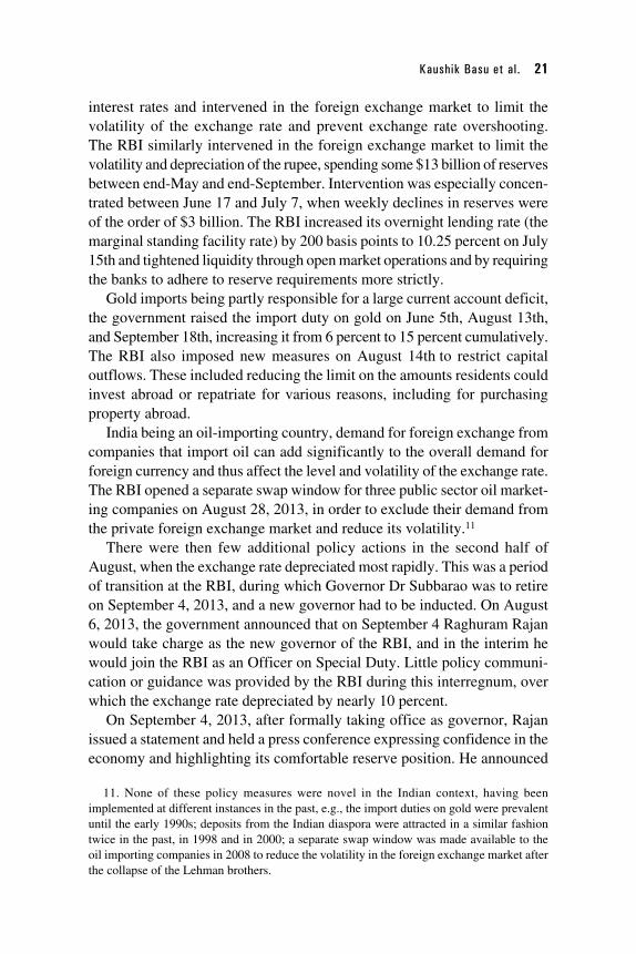
interest rates and intervened in the foreign exchange market to limit the volatility of the exchange rate and prevent exchange rate overshooting. The RBI similarly intervened in the foreign exchange market to limit the volatility and depreciation of the rupee, spending some $13 billion of reserves between end-May and end-September. Intervention was especially concen-trated between June 17 and July 7, when weekly declines in reserves were of the order of $3 billion. The RBI increased its overnight lending rate (the marginal standing facility rate) by 200 basis points to 10.25 percent on July 15th and tightened liquidity through open market operations and by requiring the banks to adhere to reserve requirements more strictly.
Gold imports being partly responsible for a large current account deficit, the government raised the import duty on gold on June 5th, August 13th, and September 18th, increasing it from 6 percent to 15 percent cumulatively. The RBI also imposed new measures on August 14th to restrict capital outflows. These included reducing the limit on the amounts residents could invest abroad or repatriate for various reasons, including for purchasing property abroad.
India being an oil-importing country, demand for foreign exchange from companies that import oil can add significantly to the overall demand for foreign currency and thus affect the level and volatility of the exchange rate. The RBI opened a separate swap window for three public sector oil market-ing companies on August 28, 2013, in order to exclude their demand from the private foreign exchange market and reduce its volatility.11
There were then few additional policy actions in the second half of August, when the exchange rate depreciated most rapidly. This was a period of transition at the RBI, during which Governor Dr Subbarao was to retire on September 4, 2013, and a new governor had to be inducted. On August 6, 2013, the government announced that on September 4 Raghuram Rajan would take charge as the new governor of the RBI, and in the interim he would join the RBI as an Officer on Special Duty. Little policy communi-cation or guidance was provided by the RBI during this interregnum, over which the exchange rate depreciated by nearly 10 percent.
On September 4, 2013, after formally taking office as governor, Rajan issued a statement and held a press conference expressing confidence in the economy and highlighting its comfortable reserve position. He announced
11. None of these policy measures were novel in the Indian context, having been implemented at different instances in the past, e.g., the import duties on gold were prevalent until the early 1990s; deposits from the Indian diaspora were attracted in a similar fashion twice in the past, in 1998 and in 2000; a separate swap window was made available to the oil importing companies in 2008 to reduce the volatility in the foreign exchange market after the collapse of the Lehman brothers.
22 IND IA POL ICY FORUM, 2014–15
new measures to attract capital through deposits targeted at nonresident Indians and partially relaxed the restrictions on outward investment intro-duced previously. Another measure that possibly helped boost the avail-ability of foreign exchange and calm the financial markets around this time was the extension of an existing swap line with Japan, which was increased from $15 billion to $50 billion. The extension of the swap line was negoti-ated between the Government of India and the Government of Japan and signed by their respective central banks.
We analyze the impact of these policy announcements on financial markets using event-study regressions. These compare the values of the exchange rate and financial market variables in a short window after the policy announcement (we report results for a five day post announcement window, but also considered shorter windows of two or three days which yielded similar results) with those prior to the announcement. For the control period, we consider two options, first, the entire tapering period from May 22 until the day of the policy announcement, and second, a shorter control period of one week prior to the announcement. Further, we report results from the specifications in which we use this shorter control period of a week.
The regression specification is given in Equation 2, in which Y is either log exchange rate, log stock market index, portfolio debt flows, or portfo-lio equity flows (portfolio flows are in millions of US$). For some policy announcements, we also look at the impact on the turnover in the foreign exchange market.
Yt = constant + µ Bond Yield in the USt + α Tapering Talk Dummyt + β Dummy for a week prior to Policy Announcementt
+ γ Dummy for Policy Announcementt + εt (2)
The regressors include US bond yields to account for global liquidity condi-tions and three separate dummies, one each for the tapering period (from May 23, 2013 until a week before the policy announcement was made), for the week prior to the policy announcement, and for the week since the policy announcement. We estimate these regressions using data from January 1, 2013, up to the date the policy dummy takes a value of 1, dropping subse-quent observations.12
12. We acknowledge the limitations in being able to establish causality using these regressions, due to the difficulty in establishing the counterfactual and in controlling for all the relevant factors that may affect the financial markets.
Kaushik Basu et al. 23
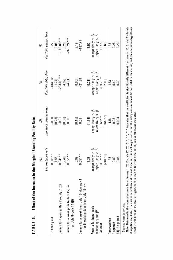
4.1. Increase in the Interest Rate (July 15)
To assess the impact of increase in interest rates on July 15, we construct the tapering dummy to take a value of 1 from May 23 to July 7, the dummy for the week prior to the announcement takes a value of 1 from July 8 to July 14, and the dummy for increase in the interest rate takes a value 1 for five consecutive days from July 15 on which the financial markets were open.
The results in Table 6 show that the rate of currency depreciation, equity prices, and debt flows did not change significantly following the increase in interest rates. It would appear, then, that this initial policy response was ineffectual.
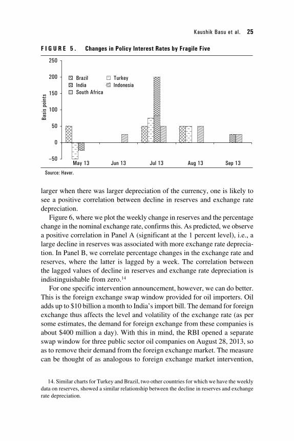
Comparing the increase in interest rates in the other Fragile Five coun-tries (Figure 5), we can see that, except for South Africa, the other coun-tries increased interest rates as well. Brazil started raising rates in May and continued doing so through the end of the year; the increase between May and September totaled 150 basis points. Indonesia first raised rates in July but continued raising them through September; the increase during May–September summed up to 100 basis points. India was different from the other countries in that it raised the interest rate by a larger amount all in one go.13 Decisiveness might be thought to signal commitment (this, pre-sumably, is what the Indian authorities had in mind). Alternatively, a large increase in rates all at once may be perceived as a sign of panic, especially if taken against the backdrop of weak fundamentals. Eichengreen and Rose (2003) suggest that sharp increases in rates designed to defend a specific level of asset prices (e.g., a specific exchange rate) may be counterproductive when nothing is done at the same time to address underlying weaknesses.
4.2. Foreign Exchange Market Intervention
The decline in reserves amounted to some $13 billion between the end of May and end of September, i.e., about 5 percent of the initial stock. Intervention was relatively large from June 17 to July 7, when reserves fell by $3 billion a week. Comparing the extent of intervention in the Fragile Five countries, we see that India and Indonesia intervened the most, and that their interven-tion was concentrated in June and July.
Not knowing the exact timing of this intervention, we are unable to run event-study regressions. Moreover, since the pressure to intervene was
13. One question of interest is whether a large one time increase is more effective, perhaps for signaling reasons, than several small increases spaced out over months.
24 IND IA POL ICY FORUM, 2011–12
TA
BL
E 6
. Ef
fect
of t
he In
crea
se in
the
Mar
gina
l Sta
ndin
g Fa
cilit
y Ra
te
(1
)(2
)(4
)(5
)
Log
exch
ange
rate
Log
stoc
k m
arke
t ind
exPo
rtfo
lio d
ebt,
$mn
Port
folio
equ
ity, $
mn
US b
ond
yiel
d0.
06**
*–0
.00
–183
.96*
9.27
[7.5
5][0
.25]
[1.7
4][0
.08]
Dum
my
for t
aper
ing
May
22–
July
7 (α
)0.
04**
*–0
.01
–233
.09*
**–1
89.8
9***
[9.4
6][0
.56]
[4.3
2][3
.20]
Dum
my
for a
wee
k pr
ior t
o Ju
ly 1
5, i.
e.
from
Jul
y 8–
July
14
(β)
0.05
***
0.00
–4.9
1–3
76.2
4***
[5.9
9][0
.15]
[0.0
5][3
.19]
Dum
my
for a
wee
k fr
om J
uly
15 (d
umm
y=1
for 5
wor
king
day
s fr
om J
uly
15) (
γ)0.
05**
*0.
02–2
1.38
–167
.71
[6.2
8][1
.34]
[0.2
1][1
.52]
Resu
lts fo
r hyp
othe
sis
com
parin
g γ
and
β#ac
cept
Ho:
γ ≥
β,
reje
ct H
a: γ
< β
acce
pt H
o: γ
≤ β
, re
ject
Ha:
γ >
βac
cept
Ho:
γ ≤
β,
reje
ct H
a: γ
> β
ac
cept
Ho:
γ ≤
β,
reje
ct H
a: γ
> β
Co
nsta
nt3.
87**
*8.
69**
*39
9.78
**13
7.50
[240
.80]
[264
.27]
[2.0
0][0
.63]
Obse
rvat
ions
135
138
133
133
R-sq
uare
d0.
890.
030.
400.
25Ad
j. R-
squa
red
0.88
0.00
40.
390.
23
Sour
ce: H
aver
Ana
lytic
s.No
te: D
ata
used
in th
e re
gres
sion
s ru
ns fr
om J
anua
ry 1
, 201
3–Ju
ly 2
2, 2
013.
*, *
*, *
** in
dica
tes
that
the
coef
ficie
nt is
sig
nific
antly
diff
eren
t fro
m ze
ro a
t 10,
5, a
nd 1
% le
vels
of s
igni
fican
ce, t
sta
tistic
s ar
e in
par
enth
eses
. # th
e nu
ll hy
poth
esis
in e
ach
regr
essi
on is
that
the
polic
y an
noun
cem
ent d
id n
ot s
tabi
lize
the
mar
ket,
and
the
alte
rnat
ive
hypo
thes
is is
that
it s
tabi
lized
it; 1
% le
vel o
f sig
nific
ance
is u
sed
to te
st th
e hy
poth
eses
, unl
ess
othe
rwis
e in
dica
ted.
Kaushik Basu et al. 25
F I G U R E 5 . Changes in Policy Interest Rates by Fragile Five
250
200
150
100
50
0
–50
Brazil Turkey India Indonesia South Africa
May 13 Jun 13 Jul 13 Aug 13 Sep 13
Basi
s po
ints
Source: Haver.
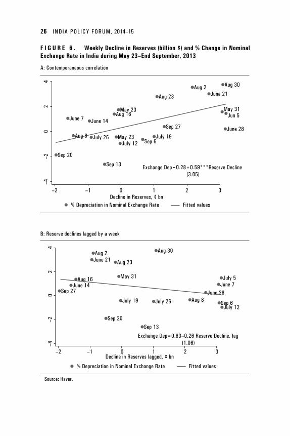
larger when there was larger depreciation of the currency, one is likely to see a positive correlation between decline in reserves and exchange rate depreciation.
Figure 6, where we plot the weekly change in reserves and the percentage change in the nominal exchange rate, confirms this. As predicted, we observe a positive correlation in Panel A (significant at the 1 percent level), i.e., a large decline in reserves was associated with more exchange rate deprecia-tion. In Panel B, we correlate percentage changes in the exchange rate and reserves, where the latter is lagged by a week. The correlation between the lagged values of decline in reserves and exchange rate depreciation is indistinguishable from zero.14
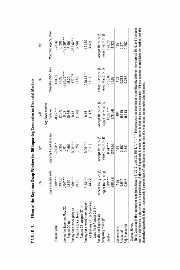
For one specific intervention announcement, however, we can do better. This is the foreign exchange swap window provided for oil importers. Oil adds up to $10 billion a month to India’s import bill. The demand for foreign exchange thus affects the level and volatility of the exchange rate (as per some estimates, the demand for foreign exchange from these companies is about $400 million a day). With this in mind, the RBI opened a separate swap window for three public sector oil companies on August 28, 2013, so as to remove their demand from the foreign exchange market. The measure can be thought of as analogous to foreign exchange market intervention,
14. Similar charts for Turkey and Brazil, two other countries for which we have the weekly data on reserves, showed a similar relationship between the decline in reserves and exchange rate depreciation.
26 IND IA POL ICY FORUM, 2014–15
F I G U R E 6 . Weekly Decline in Reserves (billion $) and % Change in Nominal Exchange Rate in India during May 23–End September, 2013
A: Contemporaneous correlation
•Aug 30•Aug 2•June 21
•June 28
•May 31•Jun 5
•Aug 23
•May 23
•June 14•June 7
•July 26 •May 23 •July 19•July 12
•Sep 27
•Sep 6•Aug 8
•Sep 20
•Sep 13
•Aug 16
–2 –1 0 1 2 3Decline in Reserves, $ bn
• % Depreciation in Nominal Exchange Rate Fitted values
–4
–2
0 2
4
Exchange Dep=0.28+0.59***Reserve Decline(3.05)
B: Reserve declines lagged by a week
•Aug 8
•Aug 23
•May 31
•Aug 30•Aug 2•June 21
•Aug 16
•Sep 27•June 14
•July 19
•Sep 20
•July 26
•Sep 13
•July 12•Sep 6
•July 5
•June 28•June 7
–2 –1 0 1 2 3Decline in Reserves lagged, $ bn
• % Depreciation in Nominal Exchange Rate Fitted values
–4
–2
0 2
4
Exchange Dep=0.83–0.26 Reserve Decline, lag(1.06)
Source: Haver.
Kaushik Basu et al. 27
where rather than intervening when the demand for foreign exchange in general increases, the RBI automatically intervenes to meet the demand from the oil companies.
Why this particular form of foreign exchange market intervention should be preferable is not entirely clear. It is not obvious whether, with a daily turnover of about $50 billion in the onshore foreign exchange market, and presumably an equally large offshore market, the amount made available through the special swap window translated into a significant reduction in the demand for foreign exchange.
While some commentators reacted positively to this announcement, we find little evidence of a favorable impact on turnover in the onshore foreign exchange market, the exchange rate or equity markets in the week follow-ing. If anything, exchange rate depreciation accelerated after this policy was announced (Table 7).
4.3. Restrictions on Capital Outflows
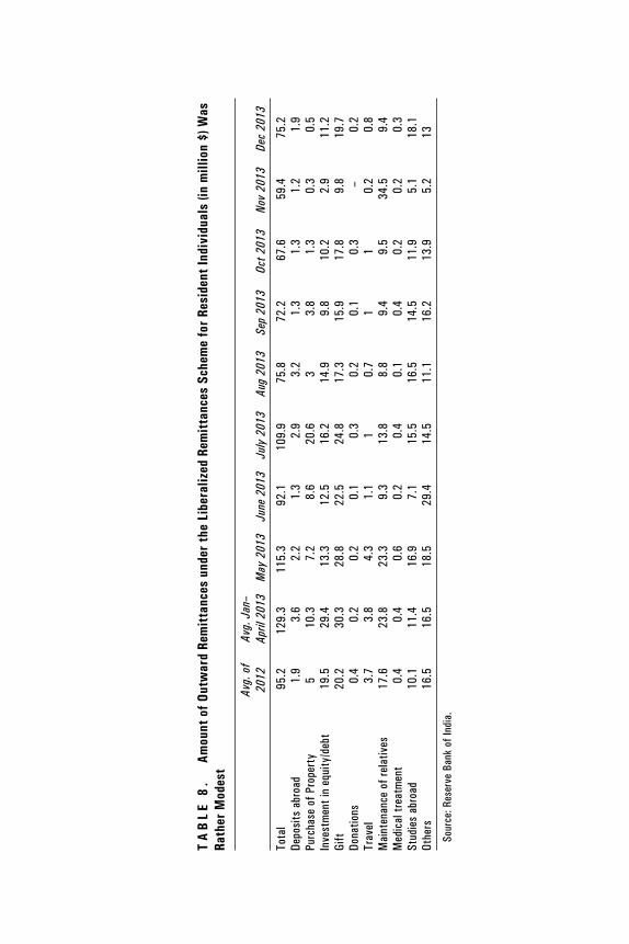
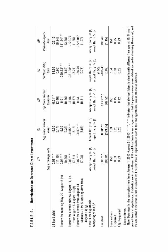
On August 14, 2013, the RBI announced restrictions on capital outflows from Indian corporates and individuals. It lowered the limit on Overseas Direct Investment under the automatic route (i.e., the outflows which do not require prior approval of the RBI) from 400 percent to 100 percent of the net worth of the Indian firms, reduced the limit on remittances by resident individuals (which were permitted under the so-called Liberalized Remittances Scheme) from $200,000 to $75,000, and discontinued remittances for acquisition of immovable property outside India. Table 8 looks at outward remittances by residents subject to these restrictions. The amounts remitted were small, of the order of $100 million a month. There was no surge in remittances during the period of tapering talk. Outflows were just $92 million in June and $110 million in July 2013. Hence there does not seem to be an apparent justification for this restriction.
Outflows once underway can be difficult to stem with these kinds of restrictions, since incentives for evasion are strong. Table 9 confirms this. Here the dummy for the tapering period prior to the restrictions takes a value of 1 from May 22 to August 6, the dummy for the week prior to policy takes a value of 1 from August 7 to August 13, while the dummy for the policy announcements takes a value of 1 for five consecutive days from August 14. The results indicate that in the five days from the time when this announce-ment was made, exchange rate depreciation and the decline in stock market index were accentuated, while equity flows declined.
Commentary in the international financial press reflected the fears that these controls evoked (The Economist, August 16, 2013, “…. India’s
28 IND IA POL ICY FORUM, 2011–12
TA
BL
E 7
. Ef
fect
of t
he S
epar
ate
Swap
Win
dow
for
Oil I
mpo
rtin
g Co
mpa
nies
on
Fina
ncia
l Mar
kets
(1
)(2
)(3
)(4
)(5
)
Log
exch
ange
rate
Log
stoc
k m
arke
t ind
exLo
g fo
rex
mar
ket
turn
over
Port
folio
deb
t, $m
nPo
rtfo
lio e
quity
, $m
n
US b
ond
yiel
d0.
09**
*–0
.03*
*–0
.22*
**11
3.02
–23.
32[1
3.15
][2
.35]
[2.8
7][1
.38]
[0.2
9]Du
mm
y fo
r tap
erin
g M
ay 2
2–Au
gust
20
(α)
0.04
***
[8.0
0]0.
01[0
.69]
0.02
[0.3
6]–2
81.7
6***
[5.2
0]–1
79.3
9***
[3.4
0]Du
mm
y fo
r a w
eek
prio
r to
Augu
st 2
8, i.
e. fr
om
Augu
st 2
1–Au
gust
27
(β)
0.09
***
–0.0
6***
0.13
–177
.07
–288
.62*
*[9
.70]
[3.2
5][1
.20]
[1.5
3][2
.56]
Dum
my
for a
wee
k fr
om A
ugus
t 28
(dum
my=
1 fo
r 5 w
orki
ng
days
from
Aug
ust 2
8) (γ
)
0.13
***
–0.0
6***
0.15
–228
.67*
*–1
71.9
2[1
4.27
][3
.11]
[1.4
7][2
.11]
[1.6
2]
Resu
lts fo
r hyp
othe
sis
com
parin
g γ
and
β#ac
cept
Ho:
γ ≥
β,
reje
ct H
a: γ
< β
acce
pt H
o: γ
≤ β
, re
ject
Ha:
γ >
βac
cept
Ho:
γ ≥
β,
reje
ct H
a: γ
< β
acce
pt H
o: γ
≤ β
, re
ject
Ha:
γ >
βac
cept
Ho:
γ ≤
β,
reje
ct H
a: γ
> β
Co
nsta
nt3.
83**
*8.
74**
*11
.33*
**-1
58.0
719
8.73
[298
.29]
[342
.55]
[76.
54]
[1.0
2][1
.32]
Obse
rvat
ions
165
168
164
162
162
R-sq
uare
d0.
944
0.35
70.
135
0.28
10.
271
Adj.
R-sq
uare
d0.
943
0.34
10.
113
0.26
30.
252
Sour
ce: H
aver
.No
te: D
ata
used
in th
e re
gres
sion
s ru
ns fr
om J
anua
ry 1
, 201
3–Ju
ly 2
2, 2
013.
*, *
*, *
** in
dica
tes
that
the
coef
ficie
nt is
sig
nific
antly
diff
eren
t fro
m ze
ro a
t 10,
5, a
nd 1
per
cent
le
vel o
f si
gnifi
canc
e, t
sta
tistic
s ar
e in
par
enth
eses
. # t
he n
ull h
ypot
hesi
s in
eac
h re
gres
sion
is t
hat
the
polic
y an
noun
cem
ent
did
not
succ
eed
in s
tabi
lizin
g th
e m
arke
t, an
d th
e al
tern
ativ
e hy
poth
esis
is th
at it
suc
ceed
ed; 1
per
cent
leve
l of s
igni
fican
ce is
use
d to
test
the
hypo
thes
es, u
nles
s ot
herw
ise
indi
cate
d.
Bharat Ramaswami and Shikha Jha 29
TA
BL
E 8
. Am
ount
of O
utw
ard
Rem
itta
nces
und
er th
e Li
bera
lized
Rem
itta
nces
Sch
eme
for
Resi
dent
Indi
vidu
als
(in m
illio
n $)
Was
Ra
ther
Mod
est
Av
g. o
f 20
12Av
g. J
an–
April
201
3M
ay 2
013
June
201
3Ju
ly 2
013
Aug
2013
Sep
2013
Oct 2
013
Nov
2013
Dec
2013
Tota
l95
.212
9.3
115.
392
.110
9.9
75.8
72.2
67.6
59.4
75.2
Depo
sits
abr
oad
1.9
3.6
2.2
1.3
2.9
3.2
1.3
1.3
1.2
1.9
Purc
hase
of P
rope
rty
510
.37.
28.
620
.63
3.8
1.3
0.3
0.5
Inve
stm
ent i
n eq
uity
/deb
t19
.529
.413
.312
.516
.214
.99.
810
.22.
911
.2Gi
ft20
.230
.328
.822
.524
.817
.315
.917
.89.
819
.7Do
natio
ns0.
40.
20.
20.
10.
30.
20.
10.
3–
0.2
Trav
el3.
73.
84.
31.
11
0.7
11
0.2
0.8
Mai
nten
ance
of r
elat
ives
17.6
23.8
23.3
9.3
13.8
8.8
9.4
9.5
34.5
9.4
Med
ical
trea
tmen
t0.
40.
40.
60.
20.
40.
10.
40.
20.
20.
3St
udie
s ab
road
10.1
11.4
16.9
7.1
15.5
16.5
14.5
11.9
5.1
18.1
Othe
rs
16.5
16.5
18.5
29.4
14.5
11.1
16.2
13.9
5.2
13
Sour
ce: R
eser
ve B
ank
of In
dia.
30 IND IA POL ICY FORUM, 2011–12
TA
BL
E 9
. R
estr
icti
ons
on O
vers
eas
Dire
ct In
vest
men
t
(1
)(2
)(3
)(4
)(5
)
Log
exch
ange
rate
Log
stoc
k m
arke
t in
dex
Log
fore
x m
arke
t tu
rnov
erPo
rtfo
lio d
ebt,
$mn
Port
folio
equ
ity,
$mn
US b
ond
yiel
d0.
08**
*–0
.00
–0.2
1**
84.9
9–2
2.13
[11.
10]
[0.1
4][2
.40]
[0.9
5][0
.24]
Dum
my
for t
aper
ing
May
22–
Augu
st 6
(α)
0.04
***
–0.0
00.
01-2
69.3
3***
–181
.64*
**[9
.26]
[0.3
3][0
.26]
[4.8
9][3
.28]
Dum
my
for a
wee
k pr
ior t
o Au
gust
14,
i.e.
fr
om A
ugus
t 7–A
ugus
t 13
(β)
0.06
***
–0.0
5***
–0.0
6-3
31.3
8***
–129
.77
[7.5
1][3
.13]
[0.5
7][3
.21]
[1.2
5]Du
mm
y fo
r a w
eek
from
Aug
ust 1
4 (d
umm
y=1
for 5
wor
king
day
s fr
om
Augu
st 1
4) (γ
)
0.07
***
–0.0
7***
0.03
–86.
70–2
28.0
4*[7
.98]
[3.9
3][0
.31]
[0.7
5][1
.97]
Resu
lts fo
r hyp
othe
sis
com
parin
g γ
and
β#Ac
cept
Ho:
γ ≥
β,
reje
ct H
a: γ
< β
Acce
pt H
o: γ
≤ β
, re
ject
Ha:
γ >
βAc
cept
Ho:
γ ≥
β,
reje
ct H
a: γ
< β
reje
ct H
o: γ
≤ β
, ac
cept
Ha:
γ >
β,
at 5
%
Acce
pt H
o: γ
≤ β
, re
ject
Ha:
γ >
β
Cons
tant
3.85
***
8.68
***
11.2
9***
–105
.41
196.
49[2
93.8
1][3
23.8
5][6
9.52
][0
.62]
[1.1
5]Ob
serv
atio
ns15
615
915
515
415
4R-
squa
red
0.93
0.25
0.15
0.31
0.25
Adj.
R-sq
uare
d0.
930.
230.
120.
290.
23
Sour
ce: H
aver
.No
te: D
ata
used
in t
he re
gres
sion
s ru
ns f
rom
Jan
uary
1, 2
013–
Augu
st 2
1, 2
013.
*, *
*, *
** in
dica
tes
that
the
coe
ffic
ient
is s
igni
fican
tly d
iffer
ent
from
zer
o at
10,
5, a
nd 1
pe
rcen
t lev
els
of s
igni
fican
ce, t
sta
tistic
s ar
e in
par
enth
eses
. # th
e nu
ll hy
poth
esis
in e
ach
regr
essi
on is
that
the
polic
y an
noun
cem
ent d
id n
ot s
ucce
ed in
sta
biliz
ing
the
mar
ket,
and
the
alte
rnat
ive
hypo
thes
is is
that
it s
ucce
eded
; 1 p
erce
nt le
vel o
f sig
nific
ance
is u
sed
to te
st th
e hy
poth
eses
, unl
ess
othe
rwis
e in
dica
ted.
Kaushik Basu et al. 31
authorities have planted a seed of doubt: might India ‘do a Malaysia’ if things get a lot worse? Malaysia famously stopped foreign investors from taking their money out of the country during a crisis in 1998…”; and Financial Times, August 15, 2013, “… the measure smacks more of desperation than of sound policy”). It is perhaps revealing that none of the other members of the Fragile Five responded to the tapering talk by restricting outflows. India’s experience suggests that they were wise.
4.4. Import Duty on Gold (June 5, August 13, and September 18)
Rising gold imports being partly responsible for the deteriorating cur-rent account balance, import duties on gold were raised from 6 percent to 8 percent on June 5 and further to 10 percent on August 13. On September 18, the duty on the imports of gold jewelry was then raised to 15 percent. Some other quantitative restrictions, such as prohibiting the import of gold coins, and a 20/80 rule requiring that 20 percent of the gold imports be made available to exporters while 80 percent could be used domestically, were introduced as well.
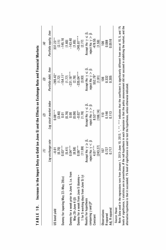
The results in Table 10 for the first duty increase on June 5 show that these duties had little positive effect. The rate of exchange rate deprecia-tion increased in the five-day window following the imposition of the duty, compared to the week before or the tapering period prior to that. The stock market declined, and portfolio inflows were smaller. These increases in import duties were ineffective because, rather than dealing with the causes of financial weaknesses, they only addressed the symptoms. Insofar as higher duties on gold imports were equivalent to tighter restraints on capi-tal outflows, they appeared to have an analogous (unfavorable) impact on financial markets.
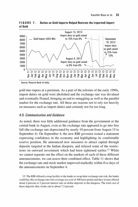
The increase in the duty on gold imports had other unintended effects as well. Even as they curtailed the import of gold (Figure 7), higher gold prices also dented exports of gold jewelry. The press reported frequent complaints from exporters about the increase in the price of gold bullion following the increase in duty. Moreover, a large difference between the domestic and international price of gold created incentives for smuggling. The World Gold Council estimated that nearly 200 tons of gold was smug-gled into India following the increase in duty (see Reuters, July 10, 2014). This is a reminder of the situation in India until the early 1990s, when due to high import duties on gold, as well as an artificially appreciated exchange rate, smuggling of gold was rampant and also contributed to a thriving parallel market for foreign exchange to convert proceeds from smuggled
32 IND IA POL ICY FORUM, 2011–12
TA
BL
E 1
0.
Incr
ease
in th
e Im
port
Dut
y on
Gol
d (o
n Ju
ne 5
) and
the
Effe
cts
on E
xcha
nge
Rate
and
Fin
anci
al M
arke
ts
(1
)(2
)(3
)(4
)
Log
exch
ange
rate
Log
stoc
k m
arke
t ind
exPo
rtfo
lio d
ebt,
$mn
Port
folio
equ
ity, $
mn
US b
ond
yiel
d–0
.01
0.08
***
–265
.42*
337.
23**
[0.7
0][3
.40]
[1.7
2][2
.11]
Dum
my
for t
aper
ing
May
22–
May
28(
α)
0.03
***
0.01
–154
.11*
–145
.16
[5.4
1][0
.76]
[1.7
7][1
.60]
Dum
my
for a
wee
k pr
ior t
o Ju
ne 5
, i.e
. fro
m
May
29–
June
4 (β
)0.
04**
*0.
00–2
31.1
8***
–143
.40
[8.5
8][0
.06]
[2.7
6][1
.65]
Dum
my
for a
wee
k fr
om J
une
5 (d
umm
y=1
for 5
wor
king
day
s fr
om J
une
5) (γ
)0.
06**
*–0
.02*
–335
.04*
**–2
45.8
7***
[11.
99]
[1.7
6][3
.93]
[2.7
7]Re
sults
for h
ypot
hesi
sco
mpa
ring
γ an
d β#
Acce
pt H
o: γ
≥ β
,re
ject
Ha:
γ <
βAc
cept
Ho:
γ ≤
β,
reje
ct H
a: γ
> β
Acce
pt H
o: γ
≤ β
,re
ject
Ha:
γ >
β
Acce
pt H
o: γ
≤ β
,re
ject
Ha:
γ >
β
Cons
tant
4.01
***
8.53
***
552.
79*
-478
.55
[243
.27]
[186
.14]
[1.9
1][1
.59]
Obse
rvat
ions
107
110
106
106
R-sq
uare
d0.
727
0.14
60.
332
0.08
8Ad
j. R-
squa
red
0.71
70.
113
0.30
50.
0516
Sour
ce: H
aver
.No
te: D
ata
used
in t
he re
gres
sion
s ru
ns f
rom
Jan
uary
1, 2
013–
June
10,
201
3. *
, **,
***
indi
cate
s th
at t
he c
oeff
icie
nt is
sig
nific
antly
diff
eren
t fr
om z
ero
at 1
0, 5
, and
1%
le
vels
of
sign
ifica
nce,
t s
tatis
tics
are
in p
aren
thes
es. #
the
null
hypo
thes
is in
eac
h re
gres
sion
is t
hat
the
polic
y an
noun
cem
ent
did
not
succ
eed
in s
tabi
lizin
g th
e m
arke
t, an
d th
e al
tern
ativ
e hy
poth
esis
is th
at it
suc
ceed
ed; 1
% le
vel o
f sig
nific
ance
is u
sed
to te
st th
e hy
poth
eses
, unl
ess
othe
rwis
e in
dica
ted.
Kaushik Basu et al. 33
gold into rupees at a premium. As a part of the reforms of the early 1990s, import duties on gold were abolished and the exchange rate was devalued and eventually floated, bringing an end to smuggling as well as the parallel market for the exchange rate. All these are reasons not to rely too heavily on measures such as import duties and certainly not for too long.
4.5. Communication and Guidance
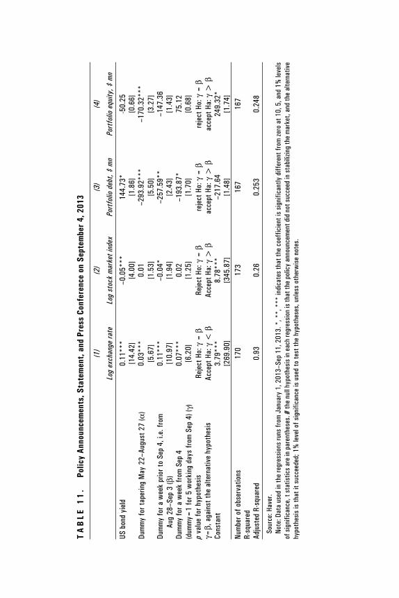
As noted, there was little additional guidance from the government or the central bank in August, even as the exchange rate appeared to go into free fall (the exchange rate depreciated by nearly 10 percent from August 15 to September 4). On September 4, the new RBI governor issued a statement expressing confidence in the economy and highlighting its comfortable reserve position. He announced new measures to attract capital through deposits targeted at the Indian diaspora, and relaxed some of the restric-tions on outward investment which had been tightened earlier.15 While we cannot separate out the effect on the markets of each of these different announcements, we can assess their combined effect. Table 11 shows that the exchange rate and stock market improved markedly within five days of the announcements on September 4.
15. The RBI offered a swap facility to the banks to swap their exchange rate risk, the banks could buy this exchange rate risk coverage at a cost of 300 basis points and they in turn offered about 4 percent or 5 percent interest rate on dollar deposits to the diaspora. The total cost of these deposits thus works out to about 7.5 percent.
F I G U R E 7 . Duties on Gold Imports Helped Restrain the (reported) Import of Gold
Dec
11Ja
n 12
Feb
12M
ar 1
2Ap
r 12
May
12
Jun
12Ju
l 12
Aug
12Se
p 12
Oct 1
2No
v 12
Dec
12Ja
n 13
Feb
13M
ar 1
3Ap
r 13
May
13
Jun
13Ju
l 13
Aug
13Se
p 13
Oct 1
3No
v 13
Dec
13
900080007000600050004000300020001000
0
September 18, 2013
Import duty on gold raised to 15% from
10%
August 13, 2013Import duty on gold raised
to 10% from 8%
August 5, 2013Import duty on gold raised
to 8% from 6%
Gold Import (US$ Mn)
Source: Reserve Bank of India.
34 IND IA POL ICY FORUM, 2011–12
TA
BL
E 1
1.
Polic
y An
noun
cem
ents
, Sta
tem
ent,
and
Pres
s Co
nfer
ence
on
Sept
embe
r 4,
201
3
(1
)(2
)(3
)(4
)
Log
exch
ange
rate
Log
stoc
k m
arke
t ind
exPo
rtfo
lio d
ebt,
$ m
nPo
rtfo
lio e
quity
, $ m
n
US b
ond
yiel
d0.
11**
*–0
.05*
**14
4.73
*-5
0.25
[14.
42]
[4.0
0][1
.86]
[0.6
6]Du
mm
y fo
r tap
erin
g M
ay 2
2–Au
gust
27
(α)
0.03
***
0.01
–293
.92*
**–1
70.3
2***
[5.6
7][1
.53]
[5.5
0][3
.27]
Dum
my
for a
wee
k pr
ior t
o Se
p 4,
i.e.
from
Au
g 28
–Sep
3 (β
)0.
11**
*–0
.04*
–257
.59*
*–1
47.3
6[1
0.97
][1
.94]
[2.4
3][1
.43]
Dum
my
for a
wee
k fr
om S
ep 4
0.
07**
*0.
02–1
93.8
7*75
.12
(dum
my=
1 fo
r 5 w
orki
ng d
ays
from
Sep
4) (
γ)[6
.20]
[1.2
5][1
.70]
[0.6
8]p
valu
e fo
r hyp
othe
sis
γ=β,
aga
inst
the
alte
rnat
ive
hypo
thes
isRe
ject
Ho:
γ =
βAc
cept
Ha:
γ <
βRe
ject
Ho:
γ =
βAc
cept
Ha:
γ >
βre
ject
Ho:
γ =
βac
cept
Ha:
γ >
βre
ject
Ho:
γ =
βac
cept
Ha:
γ >
βCo
nsta
nt3.
79**
*8.
78**
*–2
17.6
424
9.32
*[2
69.9
0][3
45.8
7][1
.48]
[1.7
4]Nu
mbe
r of o
bser
vatio
ns17
017
316
716
7R-
squa
red
Adju
sted
R-s
quar
ed0.
930.
260.
253
0.24
8
Sour
ce: H
aver
.No
te: D
ata
used
in th
e re
gres
sion
s ru
ns fr
om J
anua
ry 1
, 201
3–Se
p 11
, 201
3. *
, **,
***
indi
cate
s th
at th
e co
effic
ient
is s
igni
fican
tly d
iffer
ent f
rom
zero
at 1
0, 5
, and
1%
leve
ls of
sig
nific
ance
, t s
tatis
tics
are
in p
aren
thes
es. #
the
null
hypo
thes
is in
eac
h re
gres
sion
is th
at th
e po
licy
anno
unce
men
t did
not
suc
ceed
in s
tabi
lizin
g th
e m
arke
t, an
d th
e al
tern
ativ
e hy
poth
esis
is th
at it
suc
ceed
ed; 1
% le
vel o
f sig
nific
ance
is u
sed
to te
st th
e hy
poth
eses
, unl
ess
othe
rwis
e no
tes.
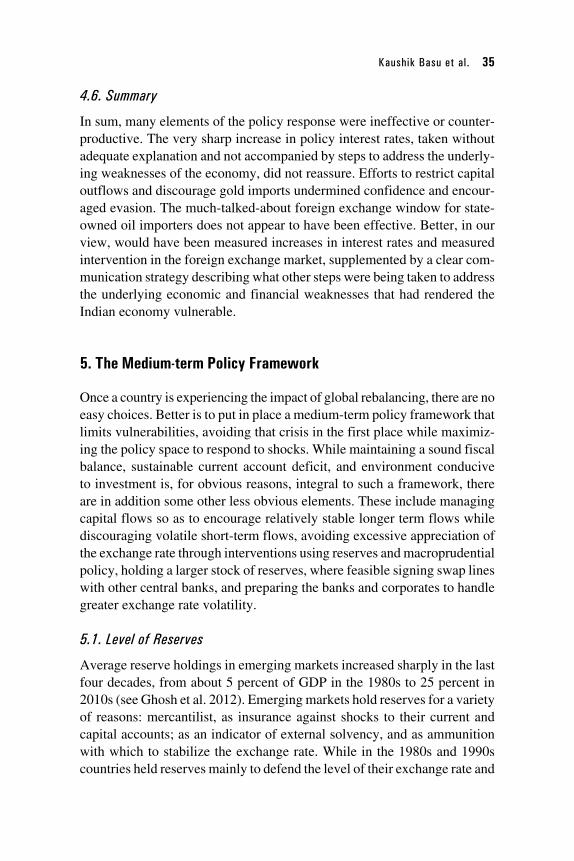
Kaushik Basu et al. 35
4.6. Summary
In sum, many elements of the policy response were ineffective or counter-productive. The very sharp increase in policy interest rates, taken without adequate explanation and not accompanied by steps to address the underly-ing weaknesses of the economy, did not reassure. Efforts to restrict capital outflows and discourage gold imports undermined confidence and encour-aged evasion. The much-talked-about foreign exchange window for state-owned oil importers does not appear to have been effective. Better, in our view, would have been measured increases in interest rates and measured intervention in the foreign exchange market, supplemented by a clear com-munication strategy describing what other steps were being taken to address the underlying economic and financial weaknesses that had rendered the Indian economy vulnerable.
5. The Medium-term Policy Framework
Once a country is experiencing the impact of global rebalancing, there are no easy choices. Better is to put in place a medium-term policy framework that limits vulnerabilities, avoiding that crisis in the first place while maximiz-ing the policy space to respond to shocks. While maintaining a sound fiscal balance, sustainable current account deficit, and environment conducive to investment is, for obvious reasons, integral to such a framework, there are in addition some other less obvious elements. These include managing capital flows so as to encourage relatively stable longer term flows while discouraging volatile short-term flows, avoiding excessive appreciation of the exchange rate through interventions using reserves and macroprudential policy, holding a larger stock of reserves, where feasible signing swap lines with other central banks, and preparing the banks and corporates to handle greater exchange rate volatility.
5.1. Level of Reserves
Average reserve holdings in emerging markets increased sharply in the last four decades, from about 5 percent of GDP in the 1980s to 25 percent in 2010s (see Ghosh et al. 2012). Emerging markets hold reserves for a variety of reasons: mercantilist, as insurance against shocks to their current and capital accounts; as an indicator of external solvency, and as ammunition with which to stabilize the exchange rate. While in the 1980s and 1990s countries held reserves mainly to defend the level of their exchange rate and
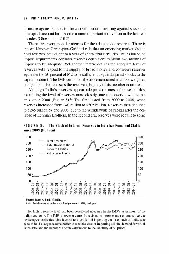
36 IND IA POL ICY FORUM, 2014–15
to insure against shocks to the current account, insuring against shocks to the capital account has become a more important motivation in the last two decades (Ghosh et al. 2012).
There are several popular metrics for the adequacy of reserves. There is the well-known Greenspan–Guidotti rule that an emerging market should hold reserves equivalent to a year of short-term liabilities. Rules based on import requirements consider reserves equivalent to about 3–6 months of imports to be adequate. Yet another metric defines the adequate level of reserves with respect to the supply of broad money and considers reserves equivalent to 20 percent of M2 to be sufficient to guard against shocks to the capital account. The IMF combines the aforementioned in a risk weighted composite index to assess the reserve adequacy of its member countries.
Although India’s reserves appear adequate on most of these metrics, examining the level of reserves more closely, one can observe two distinct eras since 2000 (Figure 8).16 The first lasted from 2000 to 2008, when reserves increased from $40 billion to $305 billion. Reserves then declined to $245 billion by end 2008, due to the withdrawals of capital after the col-lapse of Lehman Brothers. In the second era, reserves were rebuilt to some
16. India’s reserve level has been considered adequate in the IMF’s assessment of the Indian economy. The IMF is however currently revising its reserves metrics and is likely to revise upwards the desirable level of reserves for oil importing countries such as India, who need to hold a larger reserve buffer to meet the cost of importing oil, the demand for which is inelastic and the import bill often volatile due to the volatility of oil prices.
F I G U R E 8 . The Stock of External Reserves in India has Remained Stable since 2009 ($ billion)
350
300
250
200
150
100
50
0
350
300
250
200
150
100
50
0
Total Reseerves Total Reserves Net of
Forward Position Net Foreign Assets
2000
–01
2000
–09
2001
–05
2002
–01
2002
–09
2003
–05
2004
–01
2004
–09
2005
–05
2006
–01
2006
–09
2007
–05
2008
–01
2008
–09
2009
–05
2010
–01
2010
–09
2011
–05
2012
–01
2012
–09
2013
–05
2014
–01
Source: Reserve Bank of India.Note: Total reserves include net foreign assets, SDR, and gold.
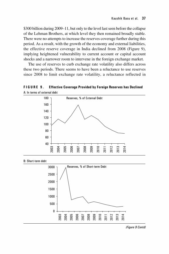
Kaushik Basu et al. 37
$300 billion during 2009–11, but only to the level last seen before the collapse of the Lehman Brothers, at which level they then remained broadly stable. There were no attempts to increase the reserves coverage further during this period. As a result, with the growth of the economy and external liabilities, the effective reserve coverage in India declined from 2008 (Figure 9), implying heightened vulnerability to current account or capital account shocks and a narrower room to intervene in the foreign exchange market.
The use of reserves to curb exchange rate volatility also differs across these two periods. There seems to have been a reluctance to use reserves since 2008 to limit exchange rate volatility, a reluctance reflected in
F I G U R E 9 . Effective Coverage Provided by Foreign Reserves has DeclinedA: In terms of external debt
Reserves, % of External Debt180
160
140
120
100
80
60
40
2003
2004
2005
2006
2007
2008
2009
2010
2011
2012
2013
2014
B: Short-term debt
Reserves, % of Short-term Debt
2003
2004
2005
2006
2007
2008
2009
2010
2011
2012
2013
2014
3000
2500
2000
1500
1000
500
0
(Figure 9 Contd)
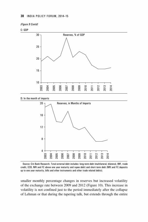
38 IND IA POL ICY FORUM, 2014–15
(Figure 9 Contd)
C: GDP
Reserves, % of GDP30
25
20
15
10
2003
2004
2005
2006
2007
2008
2009
2010
2011
2012
2013
2014
D: In the month of imports
Reserves, in Months of Imports20
16
12
8
4
2003
2004
2005
2006
2007
2008
2009
2010
2011
2012
2013
2014
Source: Citi Bank Research. Total external debt includes: long-term debt (multilateral, bilateral, IMF, trade credit, ECB, NRI and FC above one year maturity and rupee debt) and short-term debt (NRI and FC deposits up to one year maturity, bills and other instruments and other trade related debts).
smaller monthly percentage changes in reserves but increased volatility of the exchange rate between 2009 and 2012 (Figure 10). This increase in volatility is not confined just to the period immediately after the collapse of Lehman or that during the tapering talk, but extends through the entire
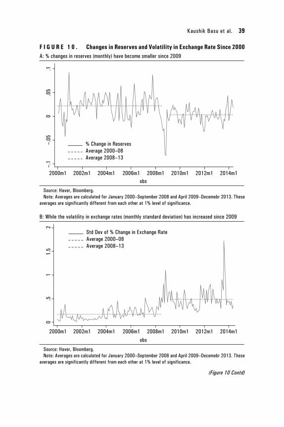
Kaushik Basu et al. 39
F I G U R E 1 0 . Changes in Reserves and Volatility in Exchange Rate Since 2000A: % changes in reserves (monthly) have become smaller since 2009
2000m1 2002m1 2004m1 2006m1 2008m1 2010m1 2012m1 2014m1obs
% Change in Reserves Average 2000–08 Average 2008–13
–.1
–.05
0
.05
.1
Source: Haver, Bloomberg.Note: Averages are calculated for January 2000–September 2008 and April 2009–Decemebr 2013. These
averages are significantly different from each other at 1% level of significance.
B: While the volatility in exchange rates (monthly standard deviation) has increased since 2009
obs
Std Dev of % Change in Exchange Rate Average 2000–08 Average 2008–13
2000m1 2002m1 2004m1 2006m1 2008m1 2010m1 2012m1 2014m1
0 .5
1
1.5
2
Source: Haver, Bloomberg.Note: Averages are calculated for January 2000–September 2008 and April 2009–Decemebr 2013. These
averages are significantly different from each other at 1% level of significance.
(Figure 10 Contd)
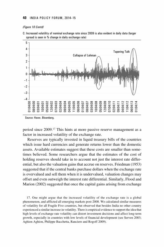
40 IND IA POL ICY FORUM, 2014–15
(Figure 10 Contd)
C: Increased volatility of nominal exchange rate since 2009 is also evident in daily data (larger spread is seen in % change in daily exchange rate)
5
4
3
2
1
0
–1
–2
–3
–4
01/0
4/00
08/0
4/00
03/0
4/01
10/0
4/01
05/0
4/02
12/0
4/02
07/0
4/03
02/0
4/04
09/0
4/04
04/0
4/05
11/0
4/05
06/0
4/06
01/0
4/07
08/0
4/07
03/0
4/08
10/0
4/08
05/0
4/09
12/0
4/09
07/0
4/10
02/0
4/11
09/0
4/11
04/0
4/12
11/0
4/12
06/0
4/13
01/0
4/14
Tapering TalkCollapse of Lehman
Source: Haver, Bloomberg.
period since 2009.17 This hints at more passive reserve management as a factor in increased volatility of the exchange rate.
Reserves are typically invested in liquid treasury bills of the countries which issue hard currencies and generate returns lower than the domestic assets. Available estimates suggest that these costs are smaller than some-times believed. Some researchers argue that the estimates of the cost of holding reserves should take in to account not just the interest rate differ-ential, but also the valuation gains that accrue on reserves. Friedman (1953) suggested that if the central banks purchase dollars when the exchange rate is overvalued and sell them when it is undervalued, valuation changes may offset and even outweigh the interest rate differential. Similarly, Flood and Marion (2002) suggested that once the capital gains arising from exchange
17. One might argue that the increased volatility of the exchange rate is a global phenomenon, and afflicted all emerging markets post-2008. We calculated similar measures of volatility for all Fragile Five countries, but observed that besides India no other country experienced a similar increase in volatility. There is empirical evidence to support the idea that high levels of exchange rate volatility can distort investment decisions and affect long-term growth, especially in countries with low levels of financial development (see Serven 2003; Aghion Aghion, Philippe Bacchetta, Ranciere and Rogoff 2009).
Kaushik Basu et al. 41
rate changes are taken into account, the opportunity cost of holding reserves is likely to be small.
World Bank (2013) estimates the cost of central bank intervention in the foreign exchange market for several emerging countries. These estimates suggest that the cost of intervention is small across countries and indeed negative for some countries. The report estimates a net gain to India from intervention in its foreign exchange market between 2005 and 2012 to be about 1 percent of its 2012 GDP.
The actual cost of intervention is likely to be even smaller than the one which accounts for the interest rate differential and the valuation effects (see Levy and Yeyati 2008), because larger reserve holdings may lower the cost of issuing sovereign or even private debt. The World Bank suggests that if the central banks still deem the cost of holding reserves to be high, they may want to consider holding a proportion of their reserves in higher yield assets, than the lower yield treasury bills, as some central banks have indeed started doing. The report reminds that, since the central banks hold reserves for a variety of reasons, the entire cost cannot be attributed to any one objective, such as to smooth exchange rate movements.
5.2. Swap Lines as a Substitute for Reserves? But Swap Line with Whom?
Since there are costs as well as benefits to holding reserves and there is no consensus on what constitutes an optimal level, bilateral swap lines with other central banks, regional swap lines such as under the Chiang Mai initiative (CMI) or Brazil, Russia, India, China and South Africa (BRICS) Contingent Reserve Arrangement (CRA), or multilateral lines such as the liquidity arrangements with the IMF may present attractive alternatives.
Eichengreen (2014) argues that, given the reluctance of the US Congress to authorize increased funding for the IMF, the Fed should contemplate extending swap lines to a larger number of emerging economies. Mohan and Kapur (2014) suggest that since monetary policies of the advanced economies have important spillovers for emerging markets, the latter ought to be offered swap facilities to limit this impact. Sheng (2014) emphasizes the need for the emerging markets to rely on swap lines, but he points out that the swap lines with the US Fed are available only selectively, and the emerging mar-kets in general do not figure in these. Hence he suggests that the emerging markets should consider a diverse set of arrangements, including signing swap arrangements with China, which has emerged as a large regional as well as global player in offering these swap lines, and pursuing regional arrangements such as the CMI or the CRA being planned by the BRICS.
42 IND IA POL ICY FORUM, 2014–15
The most recent initiative along these lines is the BRICS’s CRA, negoti-ated in summer 2014, under which the member countries committed $100 billion of reserves to the arrangement. India’s share is $18 billion, and it can withdraw twice that much from the arrangement. Just to put the size of this withdrawal facility in perspective, note that the net amount (above its own commitment to the pool) that India can withdraw is less than half the size of its current swap line with Japan and barely 5 percent of reserves. Revealingly, negotiation of an IMF program is a precondition for drawing funds from the BRICS’s CRA above the first 30 percent, just as in the CMI. The unencumbered 30 percent appears to be a rather modest amount.
The question about this arrangement is whether it will actually operate or would meet the same fate as the CMI. Participants of the CMI have been reluctant to put actual cash on the barrelhead, since they are reluctant to impose policy conditions of the sort that will maximize the likelihood of them being paid back (conditionality among neighbors being politically delicate).18 There may similarly be a reluctance to provide net resources under the CRA. While any member country can request access to the swap line up to its limit, but that request must be acceded to by the providing parties. And whether they will accede is yet to be seen.
Rajan (2014) suggests that since the IMF possesses the expertise to operate such lines, is free of political obligations to explain to the domestic stakeholders if a credit risk emerges in these arrangements, and has the capacity to bear such risks if they arise, swap arrangements should be chan-neled through it. Rajan also suggests that the IMF could act as a facilitator, helping countries identify the counterparts who would be amenable to sign-ing the bilateral or regional swap arrangements, and if needed, mediating negotiation of these swap lines. He also proposes modifications to the IMF’s existing liquidity line so as to reduce the stigma of accessing the facility and ensure its wider use by the member countries.
The countries with which India might be able to sign bilateral swap lines would perhaps be its large trading partners or the countries where foreign investment to India originates, in other words the countries which have a stake in the stability of its currency and economy. Such swap lines would be considered credible if signed with countries that are not considered to be in the same asset class as India by global investors, and thus are not likely to be affected in a similar manner by a rebalancing of global portfolios or global
18. The $100 billion of reserves are not going into a common pool. Rather, each country will continue to hold its own reserves; the commitment to provide dollars against local currency is only on paper.
Kaushik Basu et al. 43
financial conditions. Based on these considerations, some countries that India could explore bilateral swap lines with include the USA, UK, Japan, the Republic of Korea, and the countries from which India imports its oil.19
Is a swap line with the USA viable for India? Apparently the USA is very selective in offering these lines. In October 2008, the Federal Reserve Board agreed to offer liquidity swap lines to four large emerging markets, Mexico, Brazil, Singapore, and Korea. These were for $30 billion each (similar in amount to the lines offered to Canada, Sweden, and Australia). The transcripts of Federal Open Market Committee (FOMC) meetings on October 23–24, 2008, suggest that these lines were offered not just because the countries in question faced liquidity risk, but also because they were considered of systemic importance to the USA, given their financial linkages with the US economy.20 Fed officials worried that if these countries faced liquidity problems, these could spill over to the US financial institutions, given the large presence of the US financial institutions in these countries. The FOMC was also emphatic that since all of these countries held sub-stantial reserves, a large part in US treasury bonds, swap arrangements with them carried little credit risk.
Even then, the swap arrangements offered to emerging markets were less generous than those offered to the developed countries and entailed additional safeguards. Emerging markets could draw only with the prior authorization of the Fed, with individual drawings each time limited to $5 billion; central banks were required to publicly announce when they drew on their lines and to provide details of the allocation of dollar liquidity they thus obtained. And though the Fed converted the dollar swap lines put in place during the global financial crisis with the Bank of Canada, Bank of England, European Central Bank, Bank of Japan, and Swiss National Bank into longer arrangements in October 2013, the swaps with emerging markets were allowed to expire after six months.21
19. While it is difficult to anticipate what amount of additional swap lines would provide the required buffer to India in addition to its existing $300 plus billion of reserves, but perhaps something of the order of $100 billion of unconditional line would be adequate.
20. Some of these contentions are confirmed by Aizenman et al. (2010) in their empirical work conducted before these minutes were published. They established that the swap lines were offered selectively by the Fed to the countries with which the USA had substantial trade and financial linkages. The few emerging markets it offered the lines to were the ones in which the US banks had exposure; hence the USA inherently had a stake in their financial stability. Apparently India does not enjoy this advantage with the USA.
21. The amounts of swap lines with developed economies were larger, adding upto $333 billion, compared to $120 billion offered to the emerging markets. Sheng compares the arrangements signed between the Fed and these emerging markets with the swap offers that
44 IND IA POL ICY FORUM, 2014–15
There was an extensive discussion in the committee on whether any other emerging markets would be considered for swap arrangements if they approached the Fed. It acknowledged and discussed whether by selecting a small group of countries for the swap arrangements the Fed was exposing the rest of the countries, which were not offered similar arrangements, to negative market reactions. The committee decided that the swap lines would not be extended to any other emerging country, which would instead be directed to utilize a new IMF facility, which was to be announced in con-junction with the Fed’s swap line the following day. Prasad (2014) and Steil (2014) note that in 2008 the Fed rebuffed requests for swaps from Chile, the Dominican Republic, Indonesia, and Peru, and in 2012 it spurned a request from India. The swap arrangements that most emerging markets could access were with larger, more developed Asian economies such as China, Japan, and Korea, rather than with the USA, European Union, or other advanced economies (Figure 11).22
This leads us to conclude that India should not expect to rely on arrange-ments with the USA, alone or even in part, in the event of future difficulties and should seek other alternatives.
India’s only existing swap line, other than the CRA, is with Japan, as noted above. This was originally signed in 2008 for $3 billion, but was raised to $15 billion in December 2011, and again to $50 billion on September 6, 2013.23 Around the time when Japan extended its swap line with India, it also signed swap lines with Indonesia and the Philippines, and in addition was committed to swap lines to other countries in ASEAN as a part of the CMI. Given the extent of Japan’s existing commitments, there may be limits to how much further the existing India–Japan swap line can be expanded.
One multilateral option that India can consider is a precautionary facility with the IMF. As is well known, these precautionary lines of credit have been used very sparingly by the IMF members (only Mexico, Poland, and Colombia have applied). Apparently, approaching the IMF for a precau-tionary line of credit conveys an adverse signal to market participants.24
the People’s Bank of China signed with about a score of developing countries most of which export commodities to China. The latter added up to over US$426 billion, implying that the China offered a more viable alternative to developing countries than the Fed.
22. We have presented a selective list of swap lines that the Bank of China signed with other countries.
23. Our understanding is that under this agreement after the first $15bn, India can draw the rest $35 bn only after it has negotiated an IMF program.
24. A similar sentiment was recorded in the minutes of the Fed’s meetings held on October 28–29, 2008, where it was noted (by Nathan Sheets), that “ [t]hese top-tier EMEs that we are recommending for swap lines are very reluctant to return to the IMF. Given the strength of
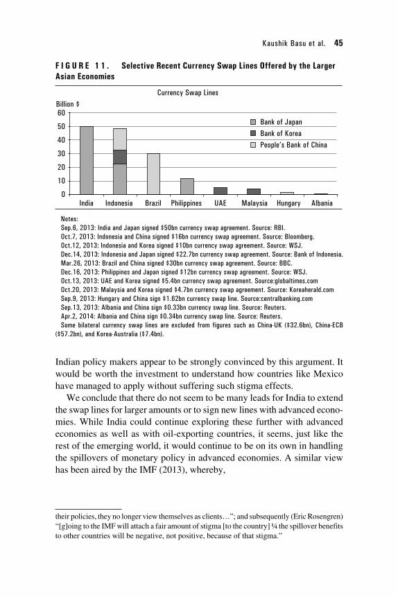
Kaushik Basu et al. 45
Indian policy makers appear to be strongly convinced by this argument. It would be worth the investment to understand how countries like Mexico have managed to apply without suffering such stigma effects.
We conclude that there do not seem to be many leads for India to extend the swap lines for larger amounts or to sign new lines with advanced econo-mies. While India could continue exploring these further with advanced economies as well as with oil-exporting countries, it seems, just like the rest of the emerging world, it would continue to be on its own in handling the spillovers of monetary policy in advanced economies. A similar view has been aired by the IMF (2013), whereby,
their policies, they no longer view themselves as clients…”; and subsequently (Eric Rosengren) “[g]oing to the IMF will attach a fair amount of stigma [to the country] ¼ the spillover benefits to other countries will be negative, not positive, because of that stigma.”
F I G U R E 1 1 . Selective Recent Currency Swap Lines Offered by the Larger Asian Economies
India Indonesia Brazil Philippines UAE Malaysia Hungary Albania
Bank of Japan Bank of Korea People’s Bank of China
Currency Swap Lines
60
50
40
30
20
10
0
Billion $
Notes:Sep.6, 2013: India and Japan signed $50bn currency swap agreement. Source: RBI.Oct.7, 2013: Indonesia and China signed $16bn currency swap agreement. Source: Bloomberg.Oct.12, 2013: Indonesia and Korea signed $10bn currency swap agreement. Source: WSJ.Dec.14, 2013: Indonesia and Japan signed $22.7bn currency swap agreement. Source: Bank of Indonesia.Mar.26, 2013: Brazil and China signed $30bn currency swap agreement. Source: BBC.Dec.16, 2013: Philippines and Japan signed $12bn currency swap agreement. Source: WSJ.Oct.13, 2013: UAE and Korea signed $5.4bn currency swap agreement. Source:globaltimes.comOct.20, 2013: Malaysia and Korea signed $4.7bn currency swap agreement. Source: Koreaherald.comSep.9, 2013: Hungary and China sign $1.62bn currency swap line. Source:centralbanking.comSep.13, 2013: Albania and China sign $0.33bn currency swap line. Source: Reuters.Apr.2, 2014: Albania and China sign $0.34bn currency swap line. Source: Reuters.Some bilateral currency swap lines are excluded from figures such as China-UK ($32.6bn), China-ECB
($57.2bn), and Korea-Australia ($7.4bn).
46 IND IA POL ICY FORUM, 2014–15
Reserves remain a critical liquidity buffer for most countries. They are generally associ-ated with lower crisis risk (crisis prevention) as well as space for authorities to respond to shocks (crisis mitigation). While other instruments, such as official credit lines and bilateral swap lines, are also external buffers, for most countries they principally act as a complement to their official reserves.25
5.3. Managing Capital Flows
Capital flows to emerging markets are volatile. However recently Bluedorn, Duttagupta, Guajardo, and Topalova (2013) noted that private capital flows are typically volatile for all countries, across all points in time, and for all types of capital flows (bank flows, portfolio debt and equity flows, etc.). They recommended using macroeconomic and macroprudential measures to buttress economic and financial resilience to such volatility.
In a similar view, in its Global Financial Stability Report, published in April 2014, the IMF acknowledged that “the reduction in US monetary accommodation could have important spillovers for advanced and emerging market economies alike as portfolios adjust and risks are repriced.” The Find noted that the increased participation of foreign investors in domestic bond markets has increased the volatility of capital flows to emerging markets. Even as the financial markets have deepened and become more globalized, new asset classes have developed, and the role of bond funds—especially local currency bond funds, open-ended funds with easy redemption options, and funds investing only opportunistically in emerging markets—has increased. These global portfolio investors and bond flows are sensitive to global financial conditions. The Fund’s recommendation, of particular rel-evance to India, is to monitor and limit the size of foreign investors in local bond markets, even as the attempts are needed to increase the participation of local investors in the bond markets.
India actively monitors and manages its capital flows. It has retained quantitative restrictions on several categories of capital inflows including on portfolio equity and debt flows. Total outstanding investment by foreign investors in government and corporate bonds are subject to different ceilings, while portfolio equity flows are subject to limits on such investment in each firm and in different sectors. India has also retained certain restrictions on capital outflows, but these apply mostly to residents. These restrictions limit the amounts that individuals can withdraw from the country each year, e.g., firms may invest abroad only up to a certain multiple of their net worth.
25. The IMF however cautions, rightly so, that the reserves cannot substitute for sound fundamentals and a good policy framework.
Kaushik Basu et al. 47
The amounts that Indian firms can borrow abroad are also monitored and, in some instances, are subject to RBI approval; and there are limits on the interest rates at which the firms can borrow abroad.
Capital flows to India consist of FDI flows, portfolio debt, and equity flows, borrowing abroad by Indian firms (called external commercial bor-rowings) and bank deposits by the Indian diaspora (often known as non-resident Indian deposits or NRI deposits). While FDI inflows and external commercial borrowings to India have been relatively stable, as has been the experience of other emerging markets, portfolio flows, and especially debt flows, into India have been more volatile (Table 12).26 This, in our view, provides some justification for the current approach of encouraging the first set of flows relative to the second.
Gordon and Gupta (2004) analyzed trends in NRI deposits and their deter-minants, and established that these deposits respond positively to the differen-tial between the interest rates on NRI deposits and what could be obtained on competing assets in other countries.27 Even though other factors affect these deposits as well, the impact of the interest rate differential outweighs that of other factors. The RBI has been repeatedly able to attract sizable amounts through special deposit schemes targeted at the nonresident population. A precedent was in 1998, when to augment its reserves (following the inter-national sanctions on India in the aftermath of nuclear tests), RBI issued the Resurgent India Bond—targeted at the NRI community, at an interest rate of 7.75 percent on US dollar deposits and raised $4.2 billion within days.
26. One potential source of vulnerability with the external commercial borrowing is the exchange rate risk that the corporates assume, exposing them to negative balance sheet effects if the exchange rate depreciates. Thus for such borrowings hedging of foreign exchange risk is important, especially for the firms which do not derive their earnings from exports.
27. NRI deposit flows to India gained momentum in the 1980s once the RBI introduced NRI deposit schemes to tap flows from the Indian diaspora abroad. It made deposits fully repatriable, offered attractive interest rates, and assumed the exchange rate risk on foreign currency-denominated accounts. However, these schemes proved to be vulnerable during the 1991 balance of payments crisis, when the outflows of deposits compounded the pressure on the external accounts. Subsequently the composition of deposits was shifted toward rupee denominated accounts; the repatriable component was reduced; and the exchange risk on foreign currency deposits was shifted to the banks. In the subsequent one decade NRI deposit inflows continued to be substantial, although their relative importance in the external accounts declined with remittances and services exports gaining pace. The authorities responded to a robust external position by linking the interest rates offered on foreign currency deposits with the Libor rate, essentially lowering the interest rates on these deposits; by giving the banks flexibility to set interest rates on rupee deposits; and by making all new deposits fully repatriable. These measures resulted in the interest rates on NRI deposits declining sharply, and moderating the inflows.
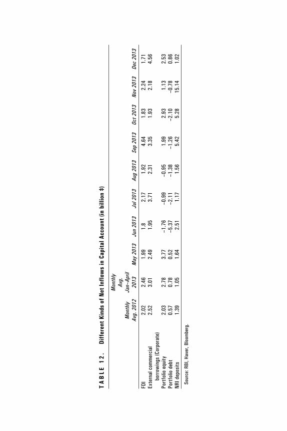
48 IND IA POL ICY FORUM, 2011–12
TA
BL
E 1
2.
Diff
eren
t Kin
ds o
f Net
Infl
ows
in C
apit
al A
ccou
nt (i
n bi
llion
$)
Mon
thly
Av
g. 2
012
Mon
thly
Av
g.
Jan–
April
20
13M
ay 2
013
Jun
2013
Jul 2
013
Aug
2013
Sep
2013
Oct 2
013
Nov
2013
Dec
2013
FDI
2.02
2.46
1.99
1.8
2.17
1.92
4.64
1.83
2.24
1.71
Exte
rnal
com
mer
cial
bo
rrow
ings
(Cor
pora
te)
2.52
3.01
2.49
1.95
3.71
2.31
3.35
1.93
2.18
4.56
Port
folio
equ
ity2.
032.
783.
77–1
.76
–0.9
9–0
.95
1.99
2.93
1.13
2.53
Port
folio
deb
t0.
570.
780.
52–5
.37
–2.1
1–1
.38
–1.2
6–2
.10
–0.7
80.
86NR
I dep
osits
1.39
1.05
1.64
2.51
1.17
1.56
5.42
5.28
15.1
41.
02
Sour
ce: R
BI, H
aver
, Blo
ombe
rg.
Kaushik Basu et al. 49
It offered a second scheme in 2000, the Indian Millennium Deposit, and was able to raise $5.5 billion at an interest rate of 8½ percent. A similar phenomenon was observed during the tapering talk episode. By providing certain incentives to the banks, the RBI managed to attract a large amount of NRI deposits through banks—net deposit mobilization was of the order of $30 billion between September and December 2013. The success implies that marketing bonds or deposits to the Indian diaspora as a crisis mitigation strategy could be deployed in the future as well.
6. Conclusion
Starting in May 2013, expectations that the Federal Reserve would begin reducing the pace of its securities purchases had a large adverse impact on emerging markets. India was among those hit hardest. Between May 22, 2013, and the end of August 2013, the rupee depreciated by 18 percent, and stock prices, foreign reserves, and portfolio flows all declined. The reaction was sufficiently pronounced for the press to warn that India might be head-ing toward a financial crisis.
Why India? Because it had received large capital flows in prior years and had large and liquid financial markets that were a convenient target for investors seeking to rebalance away from emerging markets. An addi-tional factor was that macroeconomic conditions had weakened noticeably in prior years, rendering the economy vulnerable to capital outflows and exchange rate depreciation and narrowing policy space. The deterioration in fundamentals was intertwined with the sizable amounts of capital that India imported during the period of zero interest rates and quantitative easing in the USA and other advanced economies. Rebalancing by global investors when the Fed began to talk of tapering highlighted these vulnerabilities.
The authorities adopted several measures in response, intervening in the foreign exchange market, hiking interest rates, raising the import duty on gold, introducing measures to encourage capital flows from the Indian diaspora, easing demand pressure in foreign exchange markets by opening a separate swap window for oil importing companies, and extending a swap line with the Bank of Japan. The Reserve Bank also sought to restrict capital outflows from Indian residents and companies.
Many elements of the policy response were ineffective or counter-productive. The very sharp increase in policy interest rates, taken without adequate explanation and not accompanied by steps to address the under-lying weaknesses of the economy, did not reassure the markets. Efforts to
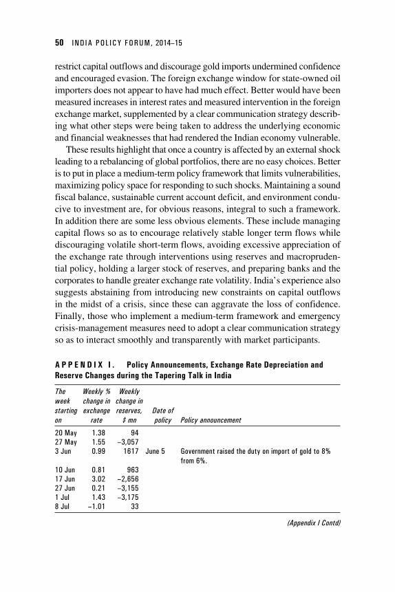
50 IND IA POL ICY FORUM, 2014–15
restrict capital outflows and discourage gold imports undermined confidence and encouraged evasion. The foreign exchange window for state-owned oil importers does not appear to have had much effect. Better would have been measured increases in interest rates and measured intervention in the foreign exchange market, supplemented by a clear communication strategy describ-ing what other steps were being taken to address the underlying economic and financial weaknesses that had rendered the Indian economy vulnerable.
These results highlight that once a country is affected by an external shock leading to a rebalancing of global portfolios, there are no easy choices. Better is to put in place a medium-term policy framework that limits vulnerabilities, maximizing policy space for responding to such shocks. Maintaining a sound fiscal balance, sustainable current account deficit, and environment condu-cive to investment are, for obvious reasons, integral to such a framework. In addition there are some less obvious elements. These include managing capital flows so as to encourage relatively stable longer term flows while discouraging volatile short-term flows, avoiding excessive appreciation of the exchange rate through interventions using reserves and macropruden-tial policy, holding a larger stock of reserves, and preparing banks and the corporates to handle greater exchange rate volatility. India’s experience also suggests abstaining from introducing new constraints on capital outflows in the midst of a crisis, since these can aggravate the loss of confidence. Finally, those who implement a medium-term framework and emergency crisis-management measures need to adopt a clear communication strategy so as to interact smoothly and transparently with market participants.
A P P E N D I X I . Policy Announcements, Exchange Rate Depreciation and Reserve Changes during the Tapering Talk in India
The week starting on
Weekly % change in exchange
rate
Weekly change in reserves,
$ mnDate of policy Policy announcement
20 May 1.38 94 27 May 1.55 –3,057 3 Jun 0.99 1617 June 5 Government raised the duty on import of gold to 8%
from 6%.10 Jun 0.81 963 17 Jun 3.02 –2,656 27 Jun 0.21 –3,155 1 Jul 1.43 –3,175 8 Jul –1.01 33
(Appendix I Contd)
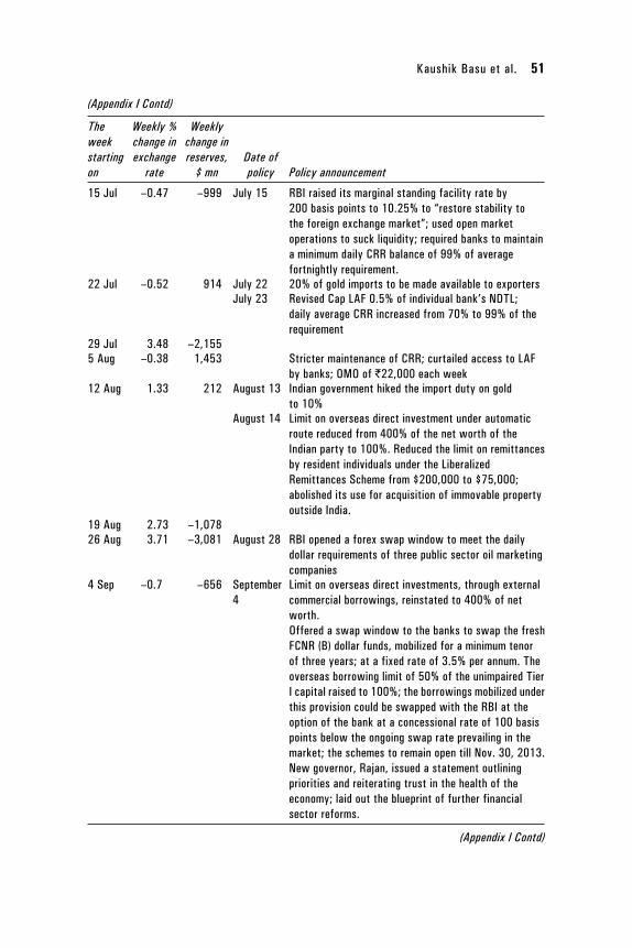
Kaushik Basu et al. 51
The week starting on
Weekly % change in exchange
rate
Weekly change in reserves,
$ mnDate of policy Policy announcement
15 Jul –0.47 –999 July 15 RBI raised its marginal standing facility rate by 200 basis points to 10.25% to “restore stability to the foreign exchange market”; used open market operations to suck liquidity; required banks to maintain a minimum daily CRR balance of 99% of average fortnightly requirement.
22 Jul –0.52 914 July 22 20% of gold imports to be made available to exporters July 23 Revised Cap LAF 0.5% of individual bank’s NDTL;
daily average CRR increased from 70% to 99% of the requirement
29 Jul 3.48 –2,1555 Aug –0.38 1,453 Stricter maintenance of CRR; curtailed access to LAF
by banks; OMO of `22,000 each week 12 Aug 1.33 212 August 13 Indian government hiked the import duty on gold
to 10% August 14 Limit on overseas direct investment under automatic
route reduced from 400% of the net worth of the Indian party to 100%. Reduced the limit on remittances by resident individuals under the Liberalized Remittances Scheme from $200,000 to $75,000; abolished its use for acquisition of immovable property outside India.
19 Aug 2.73 –1,078 26 Aug 3.71 –3,081 August 28 RBI opened a forex swap window to meet the daily
dollar requirements of three public sector oil marketing companies
4 Sep –0.7 –656 September 4
Limit on overseas direct investments, through external commercial borrowings, reinstated to 400% of net worth.Offered a swap window to the banks to swap the fresh FCNR (B) dollar funds, mobilized for a minimum tenor of three years; at a fixed rate of 3.5% per annum. The overseas borrowing limit of 50% of the unimpaired Tier I capital raised to 100%; the borrowings mobilized under this provision could be swapped with the RBI at the option of the bank at a concessional rate of 100 basis points below the ongoing swap rate prevailing in the market; the schemes to remain open till Nov. 30, 2013.New governor, Rajan, issued a statement outlining priorities and reiterating trust in the health of the economy; laid out the blueprint of further financial sector reforms.
(Appendix I Contd)
(Appendix I Contd)

52 IND IA POL ICY FORUM, 2014–15
The week starting on
Weekly % change in exchange
rate
Weekly change in reserves,
$ mnDate of policy Policy announcement
9 Sep –2.68 500 16 Sep –1.92 1975 September
18Government increased the import duty on gold jewelry to 15%
23 Sep 0.35 –1296 September 20
RBI increased the policy rate by 25 bps to 7.5%
October 7 RBI lowered the MSF rate by 50 bps to 9.0 and announced additional liquidity measures in the form of term repos of 7-day and 14-day tenor for the amount equivalent to 0.25% of banking system NDTL through variable rate auctions every Friday beginning October 11, 2013.
October 29 RBI lifted its policy repo rate by 25 bps to 7.75% November 11
RBI receives US$17.5 billion under Forex Swap Window
November 20
RBI receives US$22.7 billion under Forex Swap Window
Source: RBI, Haver, and authors' calculations.
References
Aghion, Philippe, Philippe Bacchetta, Romain Ranciere, and Kenneth Rogoff. 2009. “Exchange Rate Volatility and Productivity Growth: The Role of Financial Development,” Journal of Monetary Economics, 56(4): 494–513.
Aizenman, Joshua and Gurnain Kaur Pasricha. 2010. “Selective Swap Arrangements and the Global Financial Crisis: Analysis and Interpretation,” International Review of Economics and Finance, 19(3): 353–65.
Bluedorn, John, Rupa Duttagupta, Jaime Guajardo, and Petia Topalova. 2013. “Capital Flows are Fickle: Anytime, Anywhere,” IMF Working Paper, WP/13/183, Washington, D.C.
Cordella, Tito, Pablo Mariano Federico, Carlos A. Vegh, and Guillermo Vuletin. 2014. “ Reserve Requirements in the Brave New Macroprudential World, Brookings Institution,” World Bank Policy Research Working Paper, No. 6793, Washington, D.C.
The Economist. 2013. “Capital Controls in India, Fight the flight,” August 16, 2013. Available online at http://www.economist.com/blogs/freeexchange/2013/08/capital-controls-india (accessed on March 20, 2014).
Eichengreen, Barry. 2014. “The Dollar and the Damage Done,” February 13. Availabe online at www.project-syndicate.org/columnist/barry-eichengreen (accessed on March 25, 2014).
(Appendix I Contd)
Kaushik Basu et al. 53
Eichengreen, Barry and Poonam Gupta. 2014. “Tapering Talk: The Impact of Expectations of Reduced Federal Reserve Security Purchases on Emerging Markets,” The World Bank Policy Research Working Paper Series, No. 6754, Washington, D.C.
Eichengreen, Barry and Andrew Rose. 2003. “Does It Pay to Defend Against a Speculative Attack?” in Michael Dooley and Jeffrey Frankel, eds, Managing Currency Crises in Emerging Markets, pp. 61–82, Chicago: University of Chicago Press.
Eichengreen, Barry, Andrew Rose, Charles Wyplosz, Bernard Dumas, and Axel Weber. 1995. “Exchange Market Mayhem: The Antecedents and Aftermath of Speculative Attacks,” Economic Policy, 10(21): 249–312.
Flood, Robert and Nancy Marion. 2002. “Holding International Reserves in an Era of High Capital Mobility”, IMF Working Paper, WP/02/62, Washington, D.C.
Financial Times. 2013. “India’s Capital Crisis: Reform, not Controls, is the Only Way to Revitalize the Economy,” August 15. Available online at http://www.ft.com/intl/cms/s/0/d469362e-05af-11e3-8ed5-00144feab7de.html#axzz3AsTAQP9w (accessed on March 28, 2014).
Friedman, Milton. 1953. “The Case for Flexible Exchange Rates,” in Milton Friedman, ed., Essays in Positive Economics, pp. 157–203, Chicago: University of Chicago Press.
Ghosh, Atish, Jonathan Ostry, and Charalambos G. Tsangarides. 2012. “Shifting Motives: Explaining the Buildup in Official Reserves in Emerging Markets since the 1980s,” IMF Working Paper WP/12/34, Washington, D.C.
Gordon, James and Poonam Gupta. 2004. “Nonresident Deposits in India: In Search of Return?” Economic and Political Weekly, 39: 4165–74.
International Monetary Fund. 2013–2014. “Article IV Consultation report on various Countries,” IMF Country Report, No. 14/57, Washington DC.
Kaminsky, Graciela L., Carmen M. Reinhart, and Carlos A. Végh. 2005. “When It Rains, It Pours: Procyclical Capital Flows and Macroeconomic Policies,” NBER Macroeconomics Annual 2004, 19: 11–82, Cambridge, MA: National Bureau of Economic Research, Inc.
Kapur, Muneesh and Rakesh Mohan. 2014. “India’s Recent Macroeconomic Performance: An Assessment and Way Forward,” IMF Working Paper, WP/14/68, Washington, D.C.
Levy Yeyati, Eduardo. 2008. “The Cost of Reserves,” Economics Letters, 100(1): 39–42.
Mohan, Rakesh and Muneesh Kapur. 2014. “Monetary Policy Coordination and the Role of central Banks,” IMF Working Paper, WP/14/70, Washington, D.C.
Prasad, Eswar. 2014. The Dollar Trap: How the US Dollar Tightened its Grip on Global Finance. Princeton, NJ: Princeton University Press.
Rajan, Raghuram. 2014. “Competitive Monetary Easing: Is It Yesterday Once More?” Remarks at the Brookings Institution, Washington, D.C. Available online at http://rbi.org.in/scripts/BS_SpeechesView.aspx?Id=886 (accessed on April 14, 2014).
54 IND IA POL ICY FORUM, 2014–15
Reuters. Available online at http://in.reuters.com/article/2014/07/10/india-gold-futures-idINKBN0FF0PE20140710 (accessed on July 10, 2014).
Serven, Luis. 2002. “Real Exchange Rate Uncertainty and Private Investment in LDCs,” The review of Economics and Statistics, 85 (1): 212–18.
Sheng, Andrew. 2014. “Central Bank Currency Swaps Key to International Monetary System, East Asia Forum”. Accessed on April 10, 2014 at http://www.eastasiaforum.org/2014/04/01/central-bank-currency-swaps-key-to-international-monetary-system/.
Steil, Benn. 2014. “Taper Trouble, The International Consequences of Fed Policy,” Foreign Affairs, 93 (4): 54–61, July–August.
55
Comments and Discussion
Shankar AcharyaIndian Council for Research on International Economic Relations
Thank you Chair and thanks to the organisers for inviting me. Many thanks Poonam for a very nice presentation and a good paper too. I found the paper informative and interesting. It was particularly interesting for me to have the comparisons, both with respect of India within the context of the “fragile five,” as well as with the whole set of emerging countries, done in a profes-sional way. I think this is very important for an Indian audience because we tend to be somewhat inward looking and anything that makes us look a bit more at our neighbours or other countries to calibrate and benchmark our own experience is a very good thing.
Let me say to begin with that I agree with most of your conclusions that you presented in the last 3 or 4 slides (as presented in the conference). However, I am a little less persuaded by some of the analysis which leads to those conclusions.
Why was India impacted so severely? Frankly, I found the standard presentation with charts and sentences much more persuasive, than your econometric work. But that may be a comment on me and not on you. There is just one point which I keep repeating with apparently very little impact (see Acharya, 2012). You say somewhere that the fiscal stimulus of 2009 was one of the causes of India going downhill on the macro front. I just want to remind you and others that it was not 2009, it was 2008 and it was not fiscal “stimulus,” it was unprecedented fiscal profligacy that was carried out from a year ahead of the national elections in spring 2009. This included: the follow through on the Sixth Pay Commission’s government wage increase recommendations; the huge subsidies for oil, fertilizers, and food because of rising commodity prices and failure to undertake necessary adjustments in administered prices; the farm loan waivers announced in the 2008 budget; the ramping up of the national rural employment guarantee programme and some other things, which took the budgeted Central government fiscal deficit for fiscal 2008–09 (three quarters of which are in calendar 2008) from 2.5 percent of GDP to over 8 percent of GDP if one includes off-budget items like various kinds of bonds to petroleum and fertilizer companies.
56 IND IA POL ICY FORUM, 2014–15
This was, by a very large margin, the biggest overshooting of a budget target that Government of India has ever indulged in since its existence. It is also important to appreciate that the nature of the massive expenditure increases were not stimulus, (suggesting a possibility of withdrawal). Rather most of the expenditure hikes (government wage increases, subsidies, etc.) were of a kind which were politically difficult to scale back. Thus the “stimulus” stubbornly persisted for the next five years.
Let me move on to the policy response part. In your typology, let us start with the interest rate increases which occurred in mid-July 2013 and which you say did not seem to have much effect. I agree that in the short run they didn’t seem to have much effect in restoring external balance. In fact they might even have had the opposite effect of inducing a sense of panic in the financial markets. I think the interesting question or counterfactual here is: would it have made any difference if instead of having a 200 basis point, sharp increase in the de facto, short-term policy rates, this order of increase had been spread out over 2 or 3 months, as in some other countries. The question may be worth exploring.
On gold imports, first let me just correct you on one point, the customs duty on gold never went as high as 15 percent. There was a 15 percent rate that refered to gold jewellery, not to gold. The gold duty peaked at 10 percent during the period. I doubt this makes a big difference to your analysis but it is important to get some of these basic facts right. More broadly, to the surprise of many, the quantitative restrictions on gold imports during these several months, were quite successful in the short run in bringing down imports of gold. This, in turn, was a very important part of the compression of the 4.8 percent of GDP current account deficit in 2012–13 to below 2 percent in 2013–14. Commentators and analysts from mainstream, Anglo-Saxon traditions tend to focus on price variables but I think we should also bear in mind that sometimes non-price policy levers do serve useful purposes. Here, I refer you to the so called “80–20 scheme” which was put into place for gold jewellery makers and various other restrictions. Clearly, in a crisis, policy-makers have to be quite eclectic about choice of instruments.
On swap facilities, I agree that those to the petroleum companies were not that important in this context. The really significant measures were the swap facilities offered by the RBI in August 2013 to non resident depositors in foreign currency non-resident accounts (FCNR). Although effective in the short run in attracting capital inflows, one should not underestimate their large quasi-fiscal costs in the form of de facto exchange rate guarantees. At that time anybody in the market place knew that if you were a high net worth individual living abroad, you could borrow money at low interest,
Kaushik Basu et al. 57
invest in these FCNR deposits with high leverage and make returns of 18–20 percent. The inflows came in, but at high cost.
The other thing which helped (and which is missing in your paper) in solving the short-run mismatch between a high current account deficit and declining capital inflows was the notable modulation of “taper talk.” If you go back to the September 12 minutes of the Federal Reserve Open Market Committee and look at those, they are very soothing. They talk about a continuation of low interest rate regimes etc. In your “event analysis”, September 12 happens to fall outside the chosen “window.” But I suggest that window needs to be extended.
So, my stylized summary of the successful external liquidity crisis-management in the short run would give priority to three factors: (a) the new FCNR swap facilities; (b) the restrictive policies on gold imports, especially the non-price ones; and (c) the Fed’s softening of its taper talk stance. That is why the second half of the financial year looks much calmer according to all the financial market indicators in India.
As for the medium-term policy framework, I broadly agree with your summary recommendations. But since Indian policymakers often find it politically difficult to get the medium-term policies right, the real question is what guidance does the paper offer for handling a crisis of confidence when it occurs in the short run? I agree with the advice not to get into the difficult, near-crisis situations and that is what we keep telling our political masters all the time (from both within and outside government). But it does not seem to work! My own final thought is that in these, short-run crisis situations what works is highly sui generis and you have to feel your way as you make up an action plan. Basically, you need intelligent, flexible, and empowered policymakers at that time. And lots of luck!
Kenneth KletzerUniversity of California, Santa Cruz
This is a particularly interesting paper and a pleasure to read. The con-sequences of the reportage of Ben Bernanke’s May 22, 2013, speech on the emerging market economies provides an opportunity to analyze the vulnerability of these economies to capital flow reversals and the efficacy of policy responses. This news allows the authors to do an event study of the capital market responses across emerging markets. In their prior paper, Eichengreen and Gupta (2014) investigate how macroeconomic conditions and country-specific financial market characteristics influenced the impact
58 IND IA POL ICY FORUM, 2014–15
of the tapering talk on exchange rate depreciation, stock market indices, and international reserves. That analysis provides a nice motivation for taking the event study further to ask how India’s policy responses performed. This paper takes advantage of multiple policy announcements, specific to India, in addition to the global news shock from the Federal Reserve. I especially like this paper because the event sharply focuses on policy responses to an adverse capital market surprise.
The paper begins by observing that the effects of the tapering talk on depreciation of the rupee and central bank reserves were particularly pro-nounced in relation to the rest of the emerging market economies, although this distinction is shared by the rest of the Fragile Five. Figure 2 displays evidence for the primary conclusion of the cross-country analysis by Eichengreen and Gupta that countries with larger and more liquid capital markets suffered larger exchange rate depreciations in the months following the Bernanke speech. As expected, countries that received proportionately larger capital inflows following the US financial crisis suffered larger taper-ing talk effects. Similarly, a larger capital market as proxied by the ratio of stock market capitalization to GDP and higher market turnover ratios are positively correlated with nominal exchange rate depreciation. However, the rate of depreciation is also positively correlated with the total size of the stock of portfolio liabilities in 2012. This size effect figures prominently in the earlier paper.
How should we think about the observation that “large and liquid” mar-kets are more vulnerable? The empirical results reported in Table 5 show that absolute size matters. As explained by the authors, these effects are robust to using alternative definitions of capital market size from the reported cumulative private external financing to just GDP. Clearly, more financially open emerging markets should experience more volatile capital flows and are more vulnerable to external monetary policy shocks. Accordingly, pres-sure on exchange rates, both nominal and real, should be related to market liquidity and the relative size of a country’s financial sector. News indicating future monetary tightening by the Federal Reserve should have effects on nominal exchange rates, central bank reserves, and stock market valuations in proportion to the magnitude of the stock of external financing or other measures of financial market size as a share of GDP, controlling for market liquidity, and capital account restrictions. Table 5, along with Figure 2, shows that portfolio adjustment induced by the tapering talk concentrated on larger markets, given domestic market liquidity and relative size.
Both papers explain this, indicating that global investors rebalanced portfolios more easily and conveniently by targeting large markets. The
Kaushik Basu et al. 59
conclusion is that having a large and liquid capital market raises vulner-ability more than proportionally. That implies that one big market would be less vulnerable than many small markets in sum. Standard theories suggest that investors should move funds out of all emerging markets in propor-tion to their portfolio holdings conditioning on restrictions on or the costs of fund retrieval: that is, why should outflows as a proportion to GDP rise with GDP? Liquidity should matter for both inflows and outflows from individual emerging markets. Investment positions should reflect relative market liquidity, so that outflows ought to be roughly proportionate to external exposures. Increasing returns to portfolio rebalancing by market could explain the importance of market size in the tapering talk episode. Another, probably better, explanation for the finding is that market liquidity is being proxied by sheer size.
The primary lesson from the cross-country comparisons is that mac-roeconomic fundamentals mattered for the capital market response to the tapering talk. India was particularly vulnerable. Over the three-year period 2010–2012, India realized exceptional capital inflows and real exchange rate appreciation. The current account deficit and government deficit rose substantially after 2008. Simultaneously, the ratio of central bank reserves to money fell. By comparison to the full sample of emerging markets, India stands out with respect to inflation, public sector deficits, and public debt. These are all identifiable reasons that India was more susceptible to the announcement. A large and volatile capital inflow accompanied by real exchange rate appreciation made India a target for global portfolio adjust-ment. The large reserve decreases and nominal exchange rate depreciation reflect India’s macroeconomic exposure and limited policy space to respond to prospective monetary tightening by the Federal Reserve. The paper does a very nice and succinct job of showing this.
I now turn to the core of the paper. The event study of the policy responses to the tapering talk shock allows an assessment of how effective policy invention measures were. As we can read, several of policy responses are readily identified by an announcement of a single policy action. The analysis of these makes complete sense, and I have no criticisms of the approach or execution. Instead, I want to emphasize some of the results and implica-tions. The RBI raised the Marginal Standing Facility rate on July 15, 2013 at once. The event analysis reported in Table 6 shows that this had no effect on the dependent variables: the nominal exchange rate, stock market index, portfolio debt inflows, and portfolio equity inflows. The null hypothesis that the interest rate increase did not reduce exchange rate depreciation or capital outflows is accepted. This is certainly not a favorable finding for
60 IND IA POL ICY FORUM, 2014–15
using monetary policy as an emergency measure against an external shock. Other policy interventions include the foreign exchange swap window for oil importers, capital outflow restrictions, and gold import duty increases. The announcement of each of these did not affect the rate of exchange rate depreciation. The positive finding regarding policy interventions by the RBI is that the communication and guidance effort undertaken on September 4, 2013, did have significant stabilizing effects.
In addition to showing that the RBI’s overnight lending rate increase did not reduce exchange rate depreciation, the authors show that RBI reserve sales and the rate of depreciation are positively correlated contemporane-ously and with reserve sales lagged. Exchange intervention was not just ineffective; declining reserves appear to have contributed to diminishing market confidence. I agree with the interpretation made by the authors that short-term measures in a crisis environment did not work and with their conclusion that policy makers need to pay attention to avoiding exposure to potential external disturbances beforehand.
In the wake of the global financial crisis, the IMF suggested that capital controls could be a policy tool to contain financial contagion and manage evolving crises. The analysis of India’s experience in the summer of 2013 provided by Basu, Eichengreen, and Gupta may offer some insights on this. The tightening of controls on overseas direct investment by the RBI on August 14 did not alleviate pressure on the exchange rate or on other meas-ures of capital market pressure. I think this is a useful data point that ought to give pause to enthusiasm for keeping in place the apparatus of capital controls. Many observers reached the conclusion that India’s capital controls may have contributed to the apparent immunity of the Indian economy to contagion after the collapse of Lehman Brothers. Their argument is that having a framework in position allows authorities to raise capital account restrictions quickly in response to an unfolding crisis. That is, even though it’s always open, keeping the gate in place allows us to close it if needed.
One problem with this argument is that the evidence in favor of conclud-ing that India’s capital controls helped to insulate India from the global financial crisis is that it lacks proper evidence. The empirical findings in this paper show that tightening existing capital controls did not help mitigate the effects of an external capital market disturbance. This paper takes a clean econometric look at adjusting in-place capital controls to mitigate exchange depreciation and gets a statistically significant negative answer. This event study ought to caution policy makers that keeping the apparatus of capital controls at the ready may not be useful.
Kaushik Basu et al. 61
Given the measured failure of mitigation measures to significantly stem (or, even, not exacerbate) the fall of the rupee in the summer of 2013, the authors rightly turn attention to reforming the medium-term policy framework. The authors show that the RBI appears to have switched its international reserve policy regime in 2008 so as to systematically allow greater exchange rate volatility and lower reserve volatility. It is worthwhile noting that over the same period, the relationship between the volatility of central bank reserves and nominal exchange rate depreciation is about the same as for both Brazil and Turkey, two other members of the Fragile Five, as for India.
The rules of thumb for reserve holding have been import coverage (old rule) and short-term debt coverage (new rule). By both of these, India’s reserves were comfortably high as the rupee depreciated from June to September of 2013. Further, a glance at Figure 7 shows that reserves increased sharply as the housing market cooled in the USA and EU, then fell in the crisis and recovered a bit as capital inflows rose. These observations suggest to me that the RBI did not avail itself very much of its capacity to use reserves in the tapering talk episode. I wonder why not. A major issue, raised in this paper, is that the RBI did not make very extensive use of its reserves to resist real appreciation during 2010–12. Instead, it was restock-ing reserves from September 2008 on. An alternative and better choice of policy may have been to put reserves to use resisting real appreciation so as to protect against the consequences of eventual monetary tightening by the USA with an appreciated real exchange rate. A lesson from the effects of US monetary policy in the recession and its subsequent tapering is that central bank reserves should play an insurance role by mitigating real appreciation and rapid capital inflows, and not just be accumulated for use against rapid nominal depreciation in a crisis. I think the authors are right in arguing that a stock of reserves can be expended to avoid crises before they start. The proper role for precautionary reserves may be for use against potentially destabilizing real exchange appreciation, rather than held back to use against a destabilizing nominal depreciation.
The authors also explore the possibility of expanding international reserve swap lines. Broadening swap line participation makes tremendous sense for more efficient reserve accumulation and hoarding, as well as promot-ing policy coordination. Perhaps, more progress will come in time. A more immediate agenda for India could be to focus on managing capital inflows. The reversals in the capital account that followed the tapering talk were concentrated in portfolio flows which are much more volatile than foreign direct investment flows. Among portfolio, debt flows suffered larger and
62 IND IA POL ICY FORUM, 2014–15
more persistent reversals. As observed by the authors, managing portfolio flows should probably include policy reforms in the regulation of intermedi-aries (such as, adopting cyclical capital adequacy requirements). Maintaining a more stable macroeconomic environment and adequate policy space to avoid and manage external shocks also means using policy to reduce the volatility of short-term capital inflows and to lean against real appreciation to reduce the magnitude of capital account reversals. Managing deposits from nonresident Indians by adjusting yields so as to moderate inflows and outflows, as well as extending the maturity of inflows, is a policy opportunity for India that most other emerging markets do not have.
This is a really helpful and timely analysis. The paper makes a notable contri bution by demonstrating how the tapering event reveals the efficacy of policy interventions used to address a capital account disturbance and stem an episode of rapid nominal depreciation. The authors’ analysis of short-term policy interventions and thoughts on medium-term policy framework are important and extremely useful. Policy makers would be well advised to give these their attention.
General Discussion
Indira Rajaraman agreed that in the medium-term, we have to mainstream gold by going back to the prior duty structure. But she also supported Acharya in that it was actually the non-duty interventions to de-facilitate gold imports that were in the end more effective. There is nothing better for an exporter of gold to India than to have a major commercial bank with all its assurance of integrity be the counterpart. The removal of public sector banks as conduits for gold imports, rather than the duty hikes, was the main reason for the sharp decline in gold imports.
The second point she made was on Shankar Acharya’s comment about 2008–09, where she agreed that 2008–09 was a preelection year, sops made in the budget, and so on. But the contribution of the second set of two quar-ters in hiking the fiscal deficit over what was in place for 2007–08 was far more on account of what happened in quarters 3 and 4 after the global crisis when the fiscal stimulus kicked in than what happened in quarters 1 and 2 which was pre-stimulus.
Vijay Joshi said was that the paper would benefit by looking at financial balances. The current account deficit is the sum of public sector deficit and the private sector deficit. It is right the fiscal deficit went up, but not only did the fiscal deficit go up, but also the current account deficit worsened
Kaushik Basu et al. 63
despite the fact that private investment fell. Household financial savings also fell, which was the critical element in the current account deficit. He also emphasized the role of inflation in all this. It led to an appreciation of the real exchange rate and to the decline in household savings. If we look at the financial balances what comes out strongly is the importance of the decline in household savings as the determining factor in what happens to the current account deficit.
He also commented on the policy conclusions. Management of the capi-tal account presumably by means of capital controls etc., as an important policy instrument. In supporting that there needs to be a discussion of what India’s capital controls currently are. Quite a lot of people claim that, there are few capital controls now and that they are no longer an instrument of policy. The validity of this claim needs to be discussed. The paper implies that they can be an instrument of policy. If so, it has to say what has been happening to capital controls.
Ajay Chhibber said that the paper highlights that fact that India has drifted into a mostly open capital account. So, the question is when did this hap-pen. Was there some series of decisions that were made that got us there or did we just drift into this situation? And did the RBI really not understand what it was dealing with, that it did not have a good framework for open economy macroeconomics, did not understand the fact that all this money would come in, that the exchange rate would be appreciating and that this passive policy that was followed was really a conscious policy?
The second was linked to what Shankar Acharya said, as the paper rightly showed, the interest rate increase did not work because the big risk was FX volatility and that once this swap arrangement was put in place which took away the exchange rate risk, then of course we were able to attract the NRI and other deposits. But regarding the costs was that premium then neces-sary once we took away the foreign exchange risk? The third question was whether the persistence of inflation in any way linked to the macro stance that we have. Fourth, if we did not worry enough about the fact that the exchange rate was appreciating then, are we in a similar danger today? The Reserve Bank is buying reserves quite aggressively but at the same time we have seen a year of inflation and the rupee is still around 60, so what is the appropriate real exchange rate today. Should we be more aggressive in buying FX?
Govinda Rao referred to the paper’s proposition that the rationale for a fiscal stimulus in 2009 was the global financial crisis. He thought that it was the stimulus first and then global financial crisis came later. But, in the fiscal deficit, which increased from the budgeted 2.5 percent to 8.5 percent,
64 IND IA POL ICY FORUM, 2014–15
almost 2 percent increase was on account of the oil price increase. We had three fiscal expansion measures—the debt waiver, pay commission award, and expansion of National Employment Guarantee Act from 200 districts to 600 districts. But a much more severe shock materialized in July 2008 when crude oil prices touched $147 a barrel and then remained at an elevated level thereafter. Although there was a semblance of recovery thereafter, the inability of the policymakers to correct for the high oil prices has continued and it became a major problem, which impacted both the fiscal deficit and the current account deficit. There was a transmission from the real sector to the financial sector through this channel as well.
Abhijit Banerjee suggested a dissonance between basic macro theory and the real macroeconomics that gets done and said that this paper was an exam-ple. The fact that India had very bad macro fundamentals was known for a long time before this tightening was mooted. What was it, then, that made India and all these countries so vulnerable suddenly at that point. Somehow the level and the change are not necessarily obviously directly correlated. The paper states it as obvious that these things should align. But, the oppo-site could also have been true. India had such bad macro-fundamentals and everything that could have happened would have already happened precisely because we knew that the macro-fundamentals are bad. Therefore, any fur-ther changes would have a small effect on the economy because people who were all still holding Indian assets were people who were hedged against it. He questioned the link between bad macro-fundamentals and the claim that tightening would have a bigger effect on those economies.
Mihir Desai referred to the issue of large financial markets and how it was framed in the paper, which claims that large financial markets give the potential for more rebalancing to happen from those economies. He thought, to the contrary that large financial markets make a country more susceptible to the real exchange rate appreciations which underlie some of these problems.
He suggested that, for the event study, it would be useful to control for what other emerging markets were doing during those periods. The paper controls for the US bond yield but the premise of the paper in many ways is that we can learn from these other fragile five. So, he thought in the event study would control for, e.g., stock market data, emerging market returns ex-India so that we would then have a better sense of what is actually hap-pening idiosyncratically as a result of the policy in India.
Rajnish Mehra questioned the entire premise that the tightening actually caused any of the effects that the paper indicates. He said that quantitative easing was a reshuffle of the asset side of the balance sheets of banks. It took
Kaushik Basu et al. 65
away some bonds from there and credited it with reserves at the Fed. So, it was a pure financial transaction. Had banks taken those excess reserves and lent them out, particularly to investors in emerging markets, then it would make sense. However, for all the QE the money multiplier actually collapsed in the USA. The marginal dollar actually is sitting in the excess reserves at the Fed. On the Fed’s balance sheets, excess reserves by the banks have gone up hugely. So, he did not see the linkage between the Fed’s tightening and demand for dollars going up in the USA, causing investors to liquidate in emerging markets. He disagreed with the paper’s premise that this causation took place.
Sudipto Mundle said that the paper argues that economies should have a macroeconomic framework so that prevents crisis. Nobody can disagree with that but the fact is that countries do still get into a crisis so we have to address the question more seriously of what actually helped us get out of it at least in the short term.
He asked question was about the swap facility created for the oil compa-nies. The paper shows that if anything it may have had a negative effect. At the time when this was done there was a big recognition at least in the press that it was that action along with some other announcements that the new Governor made that began to stabilize conditions. So, why did the authors think that it did not really matter?
Surjit Bhalla thought that the paper was perilously close to concluding causation from correlation. First, the paper commented that our macro fun-damentals were very bad. So, the first counterfactual question to be asked was: Would this readjustment in the exchange rate have happened anyway? In other words, if there was no tapering, what would have happened? It may not have happened at that precise time and that is where there is no ques-tion that the tapering announcement had in effect in terms of acceleration or whatever the fundamental trends were. But after that, we need to answer that question.
Second, he said that the paper did not look at the other tapering incidents, which would have been a fantastic control to look at whether the tapering had an effect subsequently. Third, he would have liked in a cross-section study to look what the deviations were, not in a study of each country from its means etc. Inflation in India was the highest ever recorded in Indian history except for a few years after the oil crisis of 1973. We had inflation in India of 12–13 percent going on for three to four years that would immediately tell us that, all other things being equal, we would have a depreciation of the exchange rate. That happened. Therefore, if we do a cross-section study which takes into account own countries’ fundamentals relative to their trend,
66 IND IA POL ICY FORUM, 2014–15
we would find that that explains what the changes are rather than any taper-ing announcement whether in 2013 or subsequently.
Ashok Lahiri commented on the current account deterioration that we saw. He said that it was again related to the fiscal problem. If we look at public savings, if current account is a difference between savings and investment, then it is the public savings that has actually gone down quite remarkably. Coming back to the tapering, his question was: Did the RBI do anything which it would not do again if there was another crisis? Prevention is better than cure, but if we get into a crisis what the Central Bank can do is to increase interest rates, which it did, tinker with capital controls, and borrow more. He pointed out that Indian foreign exchange reserves had gone up and so had the external debt. This was basically borrowing to bol-ster reserves, along with import controls. Were the authors suggesting that the next time there is a crisis, do not increase interest rates, do not borrow more and bolster reserves, or do not try to control gold imports. What, then, should be done differently?
Seema Sangeeta expressed curiosity about the diaspora deposit policy: Whether the success of that policy was confined to India or was there any evidence of this working in the other fragile five economies or other emerg-ing markets or developing countries.
Reference
Acharya, Shankar. 2012. “India and the Global Crisis” in C. Fred Bergsten and C. Randall Henning, eds, Global Economics in Extraordinary Times, pp. 157–176. Washington, D.C.: Peterson Institute of International Economics.