Embed Size (px)
Citation preview
Ad Hoc Networks 9 (2011) 940–965
Contents lists available at ScienceDirect
Ad Hoc Networks
journal homepage: www.elsevier .com/locate /adhoc
FROMS: A failure tolerant and mobility enabled multicast routingparadigm with reinforcement learning for WSNs
Anna Förster a,⇑, Amy L. Murphy b
a NetLab, ISIN-DTI, SUPSI, Manno, Switzerlandb FBK-IRST, Trento, Italy
a r t i c l e i n f o a b s t r a c t
Article history:Received 2 February 2010Received in revised form 27 October 2010Accepted 26 November 2010Available online 9 December 2010
Keywords:Sensor networksRoutingEnergy-awareMulticastMobile sinksNode failuresReinforcement learning
1570-8705/$ - see front matter � 2010 Elsevier B.Vdoi:10.1016/j.adhoc.2010.11.006
⇑ Corresponding author.E-mail address: [email protected] (A. Förste
A growing class of wireless sensor network (WSN) applications require the use of senseddata inside the network at multiple, possibly mobile base stations. Standard WSN routingtechniques that move data from multiple sources to a single, fixed base station are notapplicable, motivating new solutions that efficiently achieve multicast and handle mobil-ity. This paper explores in depth the requirements of this set of application scenariosand proposes FROMS, a machine learning-based multicast routing paradigm. Its primarybenefits are flexibility to optimize routing over a variety of properties such as route length,battery levels, ease of recovery after node failures, and native support for sink mobility. Weprovide theoretical, simulation and experimentation results supporting these claims,showing the benefits of FROMS in terms of low routing overhead, extended network lifetime,and other key metrics for the WSN environment.
� 2010 Elsevier B.V. All rights reserved.
1. Introduction and common handheld devices and laptops into one holistic
The 1998 SmartDust [1] project is commonly used tomark the beginning of wireless sensor network (WSNs) re-search, as it identified the vision for large autonomous net-works for monitoring environmental and industrialparameters. Since then the price of individual sensors hasbeen decreasing, while memory, processing and sensoryabilities have been increasing, simultaneously expandingthe potential application scenarios. Researchers and practi-tioners from many scientific and industrial areas have al-ready leveraged the achievements of the WSN community,deploying sensor networks for applications ranging fromscientific monitoring of active volcanos [2] and glaciers[3], through agricultural and environmental monitoring[4–7], military and rescue applications [8,9], to the futuristicvision of the InterPlaNetary Internet [10,11], designed toconnect highly heterogeneous devices such as satellites,Mars and Moon rovers, sensor networks, space shuttles,
. All rights reserved.
r).
network.The growing number of applications for WSNs and their
heterogeneous requirements and properties demand newcommunication protocols and architectures. Routing forWSNs has attracted a lot of research in recent years, andmany different protocols have been developed for variousapplication scenarios and data traffic patterns. However,recently this area has attracted also criticism: applicationscenarios are too restricted or not carefully described,experimental setups are unrealistic, and simulation envi-ronments are too abstract [12]. Further, despite the over-whelming number and variety of routing protocols, keyproblems remain unsolved, important among them are en-ergy efficiency for various application scenarios and formultiple traffic patterns, as well as tolerance of failuresand mobility. Additionally, the problem of sending datato multiple, possibly mobile sinks via optimal paths (mul-ticast) has not been solved efficiently.
This paper presents a novel multicast routing protocolcalled Feedback ROuting to Multiple Sinks (FROMS),which exploits reinforcement learning. Our target scenario
A. Förster, A.L. Murphy / Ad Hoc Networks 9 (2011) 940–965 941
includes applications with periodic, long-lasting datareporting from several sources to multiple, mobile sinksin a multi-hop environment. FROMS easily accepts a rangeof cost metrics such as hops, geographic distance, latency,and remaining battery. Its most salient advantages are:
� ability to find globally optimal multicast routes;� incorporation of different cost metrics and thus optimi-
zation goals;� quick recovery in case of failures and sink mobility.
The main goal of FROMS is to provide the WSN developerwith a single routing solution, able to be tuned to many dif-ferent application scenarios.
This paper presents a comprehensive view of FROMS,including a theoretical model and an analysis of its com-plexity and overall behavior; a complete evaluation bothin simulation and on real hardware; and a challenging com-parison against both the geographic-based multicast rout-ing protocol MSTEAM [13] and a multicast variation ofDirected Diffusion [14]. The presented simulation environ-ment uses sophisticated radio propagation models and real-istic MAC protocols. In contrast to our previously reportedresults [15,16], this paper offers significantly more depthto the characterization of the FROMS parameter space andits properties, and a complete comparison to other multicastrouting protocols both in simulation and on real hardware.
Next, Section 2 motivates the work and our approach,describing major challenges and related works. Section 3gives an intuitive introduction to the FROMS routing proto-col. Sections 4 and 5 present the theoretical aspects, firstmodeling multicast routing as a reinforcement learningproblem and presenting our solution, then offering a theo-retical complexity and convergence analysis. Section 6gives a glimpse into the protocol implementation detailsbefore the simulation and testbed evaluations are dis-cussed in Sections 7–9. Finally, Sections 10 and 11 discussthe versatility of FROMS and future directions.
2. Motivation and related efforts
This section outlines the requirements and properties ofmultiple, well-known WSN deployments. We then discussthe current state-of-the-art in WSN routing protocols andhow they meet the needs and challenges of the identifiedscenario.
2.1. Target application scenario
Real WSN deployments typically follow one of twoapplication styles: periodic reporting or event detection[17]. Our focus is on the first, exemplified by disaster reliefand military applications [8,9], environmental monitoringand surveillance [2,4–7] and the InterPlaNetary Internet[10,11]. We use these applications and scenarios to guideour requirements analysis, but also extend them to incor-porate future opportunities. The following details severalkey parameters and assumptions.
Network size. Deployments range in size from a few,carefully placed nodes (e.g., volcano monitoring [2]) tohundreds of randomly placed nodes (e.g., military or disas-
ter recovery [8,9]). We target large systems with hundredsof nodes.
Data sources and sinks. An interesting class of applica-tions collects data from a subset of the nodes (possiblychanging over time), and delivers the data to a small num-ber of possibly mobile sinks. In very large deployments theset of reporting nodes is usually small (in contrast to con-vergecast applications with few nodes, all reporting), butthe data must be delivered to several, possibly mobilesinks.
Directly supporting sink mobility enables applicationssuch as disaster recovery [9] to send data directly to mobileusers inside the network, rather than collect data at a sink,then redirect it back into the network, incurring additionalcosts. This increases the reliability of the full system.
Energy constraints. One of the main advantages ofWSN nodes is freedom of placement without wiring. This,however, introduces a primary constraint: namely relianceon batteries in scenarios where replacement is difficult orimpossible. It is widely demonstrated that radio communi-cation, for both listening and sending, is the primary powerconsumer [18,19]. Therefore, data dissemination protocolsmust consider energy consumption, efficiently balancingusage throughout the network, avoiding the loss of anyportion of the network.
Node failures. Node losses are commonly caused by theexhaustion of battery reserves or hardware faults, leadingto nodes dropping out of the network. A routing frame-work must cope with such failures and guarantee continu-ous data delivery throughout the system lifetime. It shouldalso accommodate new nodes and make efficient use of allavailable resources.
Data rate and requirements. Generally data can be cat-egorized as high (e.g., from accelerometers) or low rate(e.g., from temperature sensors). We target low rates thatdo not congest the network but can fluctuate under appli-cation control.
2.2. Design and implementation requirements
In addition to application constraints, we consider sev-eral design criteria for our protocol development process,with the overall goal to ensure the real world applicabilityof our results.
Simplicity. The protocol must be easy to understandand implement, making it feasible for deployments.
Memory and processing requirements. The implemen-tation must fit onto a typical sensor node, leaving space forother protocols and applications.
Flexibility. The protocol must be adaptable to differentapplications and optimization goals, such as different costmetrics.
Scalability. The implemented protocols must be reason-ably scalable in terms of network size, number of sources,and number of sinks.
2.3. Assumptions
Our work resides at the routing layer, assuming stan-dard functionality from other components of the commu-nication stack.
942 A. Förster, A.L. Murphy / Ad Hoc Networks 9 (2011) 940–965
Sink announcements. The sink uses a simple controlledflooding mechanism to inform all network nodes about it-self and its data requirements (e.g., data type and rate).During this controlled flooding, each node sends the packetexactly once and gathers initial routing information suchas hops to the sink or sink location.
MAC layer. We assume a simple broadcast-enabledMAC protocol without re-transmissions and without deliv-ery guarantees. This class of MAC protocols is broad andmany WSN MAC protocols meet these criteria [19]. Usinga retransmission based MAC protocol is also possible, butwould require some adjustments to FROMS, as detailed inSection 10.
Neighborhood (link) management. Neighborhood man-agement protocols keep consistent information at eachnode about the identity of its neighbors as link qualitieschange and nodes fail. In this paper, we intentionally donot employ such a protocol, but instead demonstrate thatour approach alone copes with link unreliability and theassociated packet loss. Notably, however, the combinationof FROMS with a neighborhood management protocol wouldincrease the overall delivery rate by forcing FROMS to useonly good links. The implications of using a link manage-ment protocol and the needed adjustments to FROMS arediscussed in Section 10.
2.4. Related work
Many WSN routing protocols have emerged in recentyears. We first discuss traditional widely used routing pro-tocols, then focus on solutions that address the two key as-pects of our application scenario: routing to multipledestinations in large networks, mobility of those destina-tions. We also devote space to machine learning-basedtechniques.
2.4.1. Traditional WSN routingMost of the applications outlined here [2,4,5,7] use
protocols from the same family, namely MintRoute [20],MultihopLQI [21], or the Collection Tree Protocol (CTP)[22]. These protocols target convergecast scenarios, withall nodes reporting to a single static base station. Whilethey perform well in this scenario, they cannot be easilyextended to support multiple and mobile sinks. CTP, forexample, uses neighborhood beacons to update ETX-basedrouting costs to a sink and to detect loops and/or failures.Beacons are exchanged throughout entire subtrees whenrouts need to be updated. Extending this mechanism tomultiple and/or mobile sinks will likely induce beaconstorms for continuous route cost updating.
2.4.2. Multicast routing for WSNsAlthough multicast has been well studied in the re-
source constrained environment of mobile ad hoc [23]and mesh networks [24], these protocols generate an unac-ceptable amount of communication overhead to constructand maintain the routing infrastructure and thus cannot besuccessfully applied to WSNs [25].
One alternative comes with geographic routing solu-tions, which rely on the location-awareness of the nodesand use only next-hop information to route packets. For
example, GPSR [26] selects the next-hop for a packet basedon its progress to the destination in terms of distance tothe sink. A special face-routing procedure provides a mech-anism to circumnavigate void regions. GMR [27] andMSTEAM [13] provide geographic-based routing multicastsolutions, however, the resulting paths are typically longwith long, lossy hops [28], especially when void regions ex-ist. Their implementation is memory and processing inten-sive. Additionally, mobile sinks pose a major challenge tothese algorithms, since the new sink position needs to bepropagated to all network nodes.
Another approach is to adapt unicast protocols to sendto multiple destinations. Such solutions build paths froma source to each sink without explicitly considering thesharing of paths or finding globally optimal ones. Forexample, Directed Diffusion [14] can be easily extendedto support multiple sinks, but the resulting multicastroutes are not optimal.
The work described in [29] attempts to find sharedroutes from multiple sources to multiple sinks. It worksby merging next hops locally and does not explore alterna-tive routes, which can lead to sub-optimal multicastroutes. Furthermore, it does not support sink mobilitynor recovery of routes.
2.4.3. Sink mobilityWhile most routing protocols assume fixed sinks, sev-
eral solutions consider sink mobility. For example, the spa-tiotemporal mobicast routing algorithm [30] is an overlayrouting protocol that decides when to forward the datathrough a geographic routing protocol and to which neigh-bors by using the a-priori known mobility pattern of thesink. In this way it guarantees timely delivery of data toneeded regions. A similar approach is taken by Kusy et al.[31]. Unfortunately, these approaches exploit a predic-tion-based routing approach that requires a-priori infor-mation of the sink mobility and fails if the sink takes asightly different route.
In TTDD [32] the authors concentrate on efficient deliv-ery to multiple mobile sinks by clustering nodes into cells.Mobile sinks flood requests only in their local cell, and anoverlay routing approach keeps track of the current cellsof the sinks for routing data to them. While effective inhigh mobility scenarios, the overhead to build andmaintain the overlay is significant, especially in periodicreporting scenarios, which are more traffic intensive thanevent-based reporting. Therefore, TTDD is better suited toevent-detecting sensor networks with sporadic rather thancontinuous traffic.
SEAD [33] and its successor DEED [34] attempt to opti-mize routing from a single source to multiple mobile sinksby allowing each sink to select an access sensor node. A datadelivery tree is built between the source and all accessnodes based on a geographic location heuristic. When thesink moves, a path between its current nearest neighborand the access node is maintained, eliminating the needto rebuild the tree. However, if the sink moves far away,a new access node is selected and the tree is rebuilt. Theapproach shows good results in comparison to DirectedDiffusion [14] and TTDD [32] in terms of dissipated energyfor data packets. However, no evaluation of the control
A. Förster, A.L. Murphy / Ad Hoc Networks 9 (2011) 940–965 943
overhead with mobile sinks is presented, and this value isexpected to be high.
The authors of [35] present a unicast and multicast en-abled protocol for WSNs with strictly limited route lengthand memory requirements. Although the work offers solidtheoretical analysis, it has not been implemented or evenevaluated in simulation. Further, the protocol assumes sta-tic topologies and does not scale well to large networks, asit maintains routing information to a large subset of net-work nodes (not only to next-hops).
2.4.4. Machine learning-based solutionsMachine learning has gained much attention in recent
years for solving challenging problems such as routing inwireless ad hoc networks. In a recent survey, reinforce-ment learning was identified as a well-suited techniquefor routing in WSNs due to its low overhead, high flexibil-ity and robustness [36]. It has been successfully used formultiple routing problems including geographic routing[37], discovering routes between two nodes [38] and find-ing optimal compression routes in a convergecast scenario[39]. While these works show clear advantages from usingML techniques, they do impose moderate cost. Specifically,online learning of the real route costs forces the protocolsto sporadically use also longer, non-optimal routes. There-fore, ML should only be applied when the application datarequirements remain consistent for long enough to over-come the learning costs with the exploitation of the short-er, learned routes. Fortunately this is common amongmany WSN application scenarios (see also Section 2.1),making ML an appealing approach.
This paper represents the first application, to ourknowledge, of machine learning, reinforcement learningin particular, to multicast routing. As we show in theremainder of this paper, this requires the design of a newML algorithm to correctly reflect the requirements arisingfrom WSNs.
3. Protocol intuition and overview
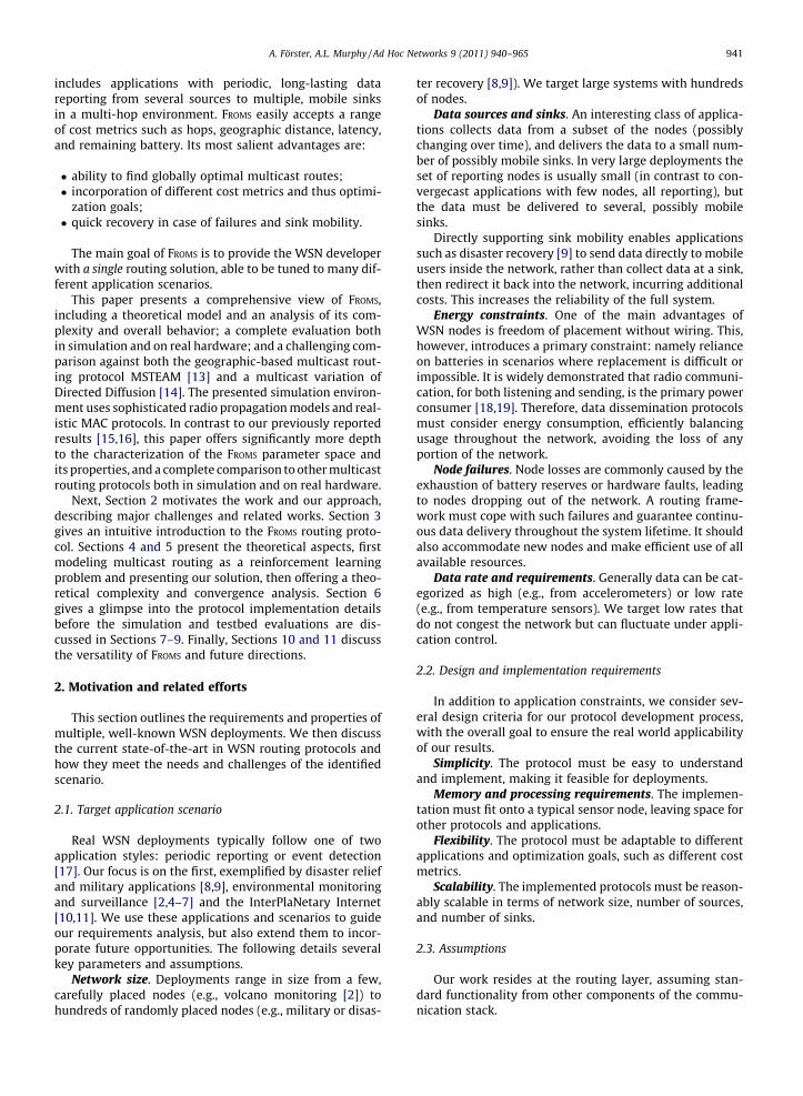
To satisfy the application needs identified in Section 2.1,our goal is to develop a protocol that finds the optimal pathfor data to follow from a source to multiple, interestedsinks. Optimal can be defined in many ways, e.g., accordingto delay, hop count, geographic distance, remaining batterylevel or any combination of the above. This section uses thenumber of hops as a simple to understand metric, whileSection 10 discusses other options in depth.
P E A
BFH
CQ
S
G
sou
sink
sink
Fig. 1. A sample topology with 2 sinks, the main routes
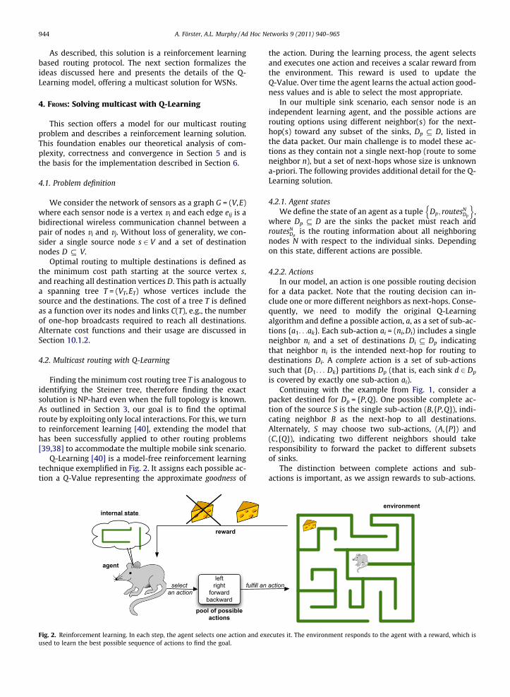
To illustrate the potential benefits from identifying theoptimal route, consider the sample network in Fig. 1 withone source and two sinks. One possible path from thesource to the sinks is formed by the union of the individualshortest paths from the source to each sink (the dottedlines in the figure). However going through nodes B, Fand H yields a shorter route. The challenge is to identifythis route without full topology information. The main taskof our protocol is to exchange next-hop routing informationamong neighbors such that the optimal route is discovered.
Using Fig. 1 as an example, the main functionality of ourprotocol is as follows. An initial sink announcement phaseallows all nodes to gather preliminary routing informationtoward sinks. As shown, S gathers individual hop counts foreach sink through each neighbor (right table in Fig. 1).When a data packet arrives, a node must select one ormore nodes to serve as the next hop(s) towards the desti-nations. While a node could simply choose the best nodeswith the shortest individual paths (in our example: C toreach sink Q and A to reach sink P), the node optionally ex-plores non-optimal routes based on the assumption thatthese might have lower costs than those calculated fromthe individual costs in the routing table. Such lower costsarise because neighboring nodes may be able to share sub-sequent hops to reach the sinks.
To show how information about the shorter paths prop-agates, consider that initially S estimates that node A re-quires 7 hops to reach both sinks: 3 hops to sink P, 5hops to sink Q and the first hop is shared (removing 1 fromthe total). However, A’s initial estimate to reach both sinksthrough E is only (2 + 4) � 1 = 5 hops, implying that S canreach both sinks though A in 6 hops (the 5 hops of A plusthe one hop from S to A). By propagating the cost of 5 fromA to S, S can update its routing estimate. This information ispiggybacked on all data packets. Therefore, by exploitingthe broadcast environment, data can be simultaneouslysent to E and routing information propagated back to S.Similarly, E piggybacks its cost estimate, informing A, andso on.
We observe that piggybacked values, which we callfeedback, propagate backward in the direction from thesink to the source. Therefore, for accurate hop count infor-mation to arrive at the source, multiple packets must besent down the same path. Further, a node must send pack-ets to all neighboring nodes to explore all possible pathsfor their real costs. We also note that keeping all routesat all nodes and always supplying current cost estimationas feedback innately allows our protocol to support recov-ery of failed nodes and mobility.
rce
Neighbor A
routing table : node S
sink P 3 hops
sink Q 5 hops
Neighbor B sink P 4 hops
sink Q 4 hops
Neighbor C sink P 5 hops
sink Q 3 hops
to them from source S and its initial routing table.
944 A. Förster, A.L. Murphy / Ad Hoc Networks 9 (2011) 940–965
As described, this solution is a reinforcement learningbased routing protocol. The next section formalizes theideas discussed here and presents the details of the Q-Learning model, offering a multicast solution for WSNs.
4. FROMS: Solving multicast with Q-Learning
This section offers a model for our multicast routingproblem and describes a reinforcement learning solution.This foundation enables our theoretical analysis of com-plexity, correctness and convergence in Section 5 and isthe basis for the implementation described in Section 6.
4.1. Problem definition
We consider the network of sensors as a graph G = (V,E)where each sensor node is a vertex vi and each edge eij is abidirectional wireless communication channel between apair of nodes vi and vj. Without loss of generality, we con-sider a single source node s 2 V and a set of destinationnodes D # V.
Optimal routing to multiple destinations is defined asthe minimum cost path starting at the source vertex s,and reaching all destination vertices D. This path is actuallya spanning tree T = (VT,ET) whose vertices include thesource and the destinations. The cost of a tree T is definedas a function over its nodes and links C(T), e.g., the numberof one-hop broadcasts required to reach all destinations.Alternate cost functions and their usage are discussed inSection 10.1.2.
4.2. Multicast routing with Q-Learning
Finding the minimum cost routing tree T is analogous toidentifying the Steiner tree, therefore finding the exactsolution is NP-hard even when the full topology is known.As outlined in Section 3, our goal is to find the optimalroute by exploiting only local interactions. For this, we turnto reinforcement learning [40], extending the model thathas been successfully applied to other routing problems[39,38] to accommodate the multiple mobile sink scenario.
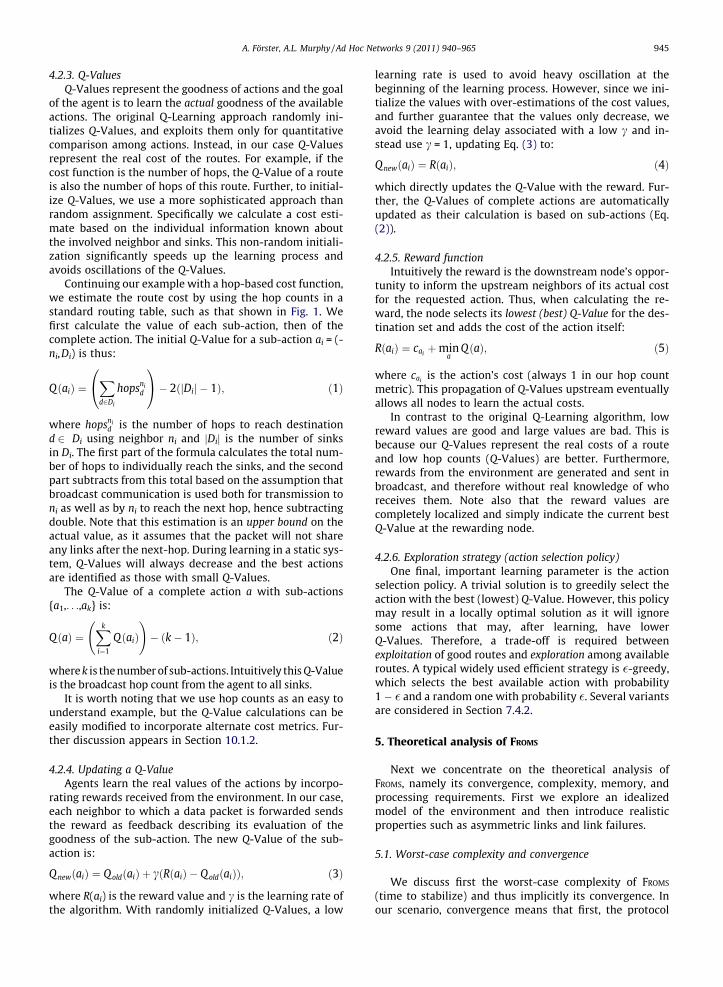
Q-Learning [40] is a model-free reinforcement learningtechnique exemplified in Fig. 2. It assigns each possible ac-tion a Q-Value representing the approximate goodness of
leftright
forwardbackward
pool of possibleactions
select an action
ll an
reward
agent
internal state
Fig. 2. Reinforcement learning. In each step, the agent selects one action and exused to learn the best possible sequence of actions to find the goal.
the action. During the learning process, the agent selectsand executes one action and receives a scalar reward fromthe environment. This reward is used to update theQ-Value. Over time the agent learns the actual action good-ness values and is able to select the most appropriate.
In our multiple sink scenario, each sensor node is anindependent learning agent, and the possible actions arerouting options using different neighbor(s) for the next-hop(s) toward any subset of the sinks, Dp # D, listed inthe data packet. Our main challenge is to model these ac-tions as they contain not a single next-hop (route to someneighbor n), but a set of next-hops whose size is unknowna-priori. The following provides additional detail for the Q-Learning solution.
4.2.1. Agent statesWe define the state of an agent as a tuple Dp; routesN
Dp
n o,
where Dp # D are the sinks the packet must reach androutesN
Dpis the routing information about all neighboring
nodes N with respect to the individual sinks. Dependingon this state, different actions are possible.
4.2.2. ActionsIn our model, an action is one possible routing decision
for a data packet. Note that the routing decision can in-clude one or more different neighbors as next-hops. Conse-quently, we need to modify the original Q-Learningalgorithm and define a possible action, a, as a set of sub-ac-tions {a1. . .ak}. Each sub-action ai = (ni,Di) includes a singleneighbor ni and a set of destinations Di # Dp indicatingthat neighbor ni is the intended next-hop for routing todestinations Di. A complete action is a set of sub-actionssuch that {D1. . . Dk} partitions Dp (that is, each sink d 2 Dp
is covered by exactly one sub-action ai).Continuing with the example from Fig. 1, consider a
packet destined for Dp = {P,Q}. One possible complete ac-tion of the source S is the single sub-action (B, {P,Q}), indi-cating neighbor B as the next-hop to all destinations.Alternately, S may choose two sub-actions, (A, {P}) and(C, {Q}), indicating two different neighbors should takeresponsibility to forward the packet to different subsetsof sinks.
The distinction between complete actions and sub-actions is important, as we assign rewards to sub-actions.
action
environment
ecutes it. The environment responds to the agent with a reward, which is
A. Förster, A.L. Murphy / Ad Hoc Networks 9 (2011) 940–965 945
4.2.3. Q-ValuesQ-Values represent the goodness of actions and the goal
of the agent is to learn the actual goodness of the availableactions. The original Q-Learning approach randomly ini-tializes Q-Values, and exploits them only for quantitativecomparison among actions. Instead, in our case Q-Valuesrepresent the real cost of the routes. For example, if thecost function is the number of hops, the Q-Value of a routeis also the number of hops of this route. Further, to initial-ize Q-Values, we use a more sophisticated approach thanrandom assignment. Specifically we calculate a cost esti-mate based on the individual information known aboutthe involved neighbor and sinks. This non-random initiali-zation significantly speeds up the learning process andavoids oscillations of the Q-Values.
Continuing our example with a hop-based cost function,we estimate the route cost by using the hop counts in astandard routing table, such as that shown in Fig. 1. Wefirst calculate the value of each sub-action, then of thecomplete action. The initial Q-Value for a sub-action ai = (-ni,Di) is thus:
QðaiÞ ¼Xd2Di
hopsnid
0@
1A� 2ðjDij � 1Þ; ð1Þ
where hopsnid is the number of hops to reach destination
d 2 Di using neighbor ni and jDij is the number of sinksin Di. The first part of the formula calculates the total num-ber of hops to individually reach the sinks, and the secondpart subtracts from this total based on the assumption thatbroadcast communication is used both for transmission toni as well as by ni to reach the next hop, hence subtractingdouble. Note that this estimation is an upper bound on theactual value, as it assumes that the packet will not shareany links after the next-hop. During learning in a static sys-tem, Q-Values will always decrease and the best actionsare identified as those with small Q-Values.
The Q-Value of a complete action a with sub-actions{a1,. . .,ak} is:
QðaÞ ¼Xk
i¼1
QðaiÞ !
� ðk� 1Þ; ð2Þ
where k is the number of sub-actions. Intuitively this Q-Valueis the broadcast hop count from the agent to all sinks.
It is worth noting that we use hop counts as an easy tounderstand example, but the Q-Value calculations can beeasily modified to incorporate alternate cost metrics. Fur-ther discussion appears in Section 10.1.2.
4.2.4. Updating a Q-ValueAgents learn the real values of the actions by incorpo-
rating rewards received from the environment. In our case,each neighbor to which a data packet is forwarded sendsthe reward as feedback describing its evaluation of thegoodness of the sub-action. The new Q-Value of the sub-action is:
Q newðaiÞ ¼ QoldðaiÞ þ cðRðaiÞ � QoldðaiÞÞ; ð3Þ
where R(ai) is the reward value and c is the learning rate ofthe algorithm. With randomly initialized Q-Values, a low
learning rate is used to avoid heavy oscillation at thebeginning of the learning process. However, since we ini-tialize the values with over-estimations of the cost values,and further guarantee that the values only decrease, weavoid the learning delay associated with a low c and in-stead use c = 1, updating Eq. (3) to:
Q newðaiÞ ¼ RðaiÞ; ð4Þ
which directly updates the Q-Value with the reward. Fur-ther, the Q-Values of complete actions are automaticallyupdated as their calculation is based on sub-actions (Eq.(2)).
4.2.5. Reward functionIntuitively the reward is the downstream node’s oppor-
tunity to inform the upstream neighbors of its actual costfor the requested action. Thus, when calculating the re-ward, the node selects its lowest (best) Q-Value for the des-tination set and adds the cost of the action itself:
RðaiÞ ¼ caiþmin
aQðaÞ; ð5Þ
where caiis the action’s cost (always 1 in our hop count
metric). This propagation of Q-Values upstream eventuallyallows all nodes to learn the actual costs.
In contrast to the original Q-Learning algorithm, lowreward values are good and large values are bad. This isbecause our Q-Values represent the real costs of a routeand low hop counts (Q-Values) are better. Furthermore,rewards from the environment are generated and sent inbroadcast, and therefore without real knowledge of whoreceives them. Note also that the reward values arecompletely localized and simply indicate the current bestQ-Value at the rewarding node.
4.2.6. Exploration strategy (action selection policy)One final, important learning parameter is the action
selection policy. A trivial solution is to greedily select theaction with the best (lowest) Q-Value. However, this policymay result in a locally optimal solution as it will ignoresome actions that may, after learning, have lowerQ-Values. Therefore, a trade-off is required betweenexploitation of good routes and exploration among availableroutes. A typical widely used efficient strategy is �-greedy,which selects the best available action with probability1 � � and a random one with probability �. Several variantsare considered in Section 7.4.2.
5. Theoretical analysis of FROMS
Next we concentrate on the theoretical analysis ofFROMS, namely its convergence, complexity, memory, andprocessing requirements. First we explore an idealizedmodel of the environment and then introduce realisticproperties such as asymmetric links and link failures.
5.1. Worst-case complexity and convergence
We discuss first the worst-case complexity of FROMS
(time to stabilize) and thus implicitly its convergence. Inour scenario, convergence means that first, the protocol
946 A. Förster, A.L. Murphy / Ad Hoc Networks 9 (2011) 940–965
is stable and the Q-Values no longer change, and secondand more importantly, that the optimal route has beenidentified. The original Q-Learning algorithm has beenshown to converge after an infinite number of steps [41].Here we need to show that our Q-Learning based protocolconverges after a finite number of steps. For this, we startby calculating the number of steps until convergence.
First, we assume a Q-Learning algorithm such as the onejust presented in Section 4 with c = 1, a hop-based costmetric, and a deterministic exploration strategy thatchooses routes in a round-robin manner. We further as-sume a network with nodes in the set N with the followingproperties, summarized in Table 1: D is the number of des-tinations, M is the diameter N (the longest shortest pathbetween any two nodes in N) and Y is the maximum den-sity of N (the maximum number of 1-hop neighbors of anynode in N). We assume stationary nodes and sinks and per-fect, stable communication among neighbors. Without lossof generality, we assume a single source. This is possiblebecause the routes are constructed depending on the des-tinations, not on the sources. Nevertheless, we discussmultiple sources at the end of this section.
The maximum number of possible actions A at any nodeis, according to the definition of actions in Section 4, thenumber of permutations of size D over a maximum of Yneighbors with repetitions (because we can use the sameneighbor to reach multiple sinks) or:
A 6 YD: ð6ÞIn the worst case the source of the data, the initiator of
the learning process, is at the maximum distance M fromall of the sinks. Our goal is to compute how many actionselection steps must be taken by all nodes in N, such thatthe Q-Values stabilize to the optimal, minimum cost. Withc = 1 the feedback of any 1-hop neighbor directly replacesthe old Q-Value. Thus, to learn the real cost of any route oflength M we need exactly M-1 steps, as the real cost prop-agates backward from the destination one step each timethe path is used. However, the source must wait for allother nodes to stabilize their Q-Values before it can beguaranteed that its Q-Values are also stable. In the worstcase it must fully explore all possible routes in the wholenetwork.
To count the number of action selection steps S for thewhole system to converge we assume the learning is initi-ated by the source, and by the previous reasoning we knowthat we must select each of the available routes M-1 times.Using Eq. (6) we have:
S 6 ðM � 1Þ � YD:
Table 1Summary of network scenario and complexity parameters.
Parameter Description
jNj Number of nodes in the network ND Number of destinationsM Network diameterY Maximum network density (maximum number of 1-
hop neighbors)A Maximum number of possible actions at each nodeS Maximum number of action steps (sent packets) at the
source before convergence
The 1-hop neighbors of the source must do the same. Theirdistance to the sinks is also at most M. Note this is theworst case and in a real network it cannot be the case thatall nodes are M hops away from the sinks: if all neighborsof some node are at the same distance from the sinks as thenode itself, the network is disconnected. Thus, all nodesmust select each of their routes at most M times and forthe complexity, we have:
S 6 ðM � 1Þ � jNj � YD ¼ O ðM � 1Þ � jNj � YD� �
: ð7Þ
This is the worst-case number of actions across all nodes(packet broadcasts) for the protocol to converge. After con-vergence, exploration can be stopped and the algorithmcan proceed in a greedy mode, as the best, optimal, routehas been identified as that with the lowest Q-Value. If morethan one route have the same Q-Value, a node can alter-nate between them to spread energy expenditure.
This, admittedly, is a very loose upper bound of thecomplexity as no real networks have the worst-case prop-erties such as all neighbors being M hops away from the des-tinations. On the other hand, this analysis does offer an ideaof scalability and expected performance. In the next para-graphs we discuss how the convergence behavior changeswith various network parameters and the consequencesfor the protocol. Later, in Sections 7–9, we use experimen-tal evaluations to show the real behavior of the protocol.
5.1.1. Parameter analysisThe number of destinations D and the density Y are nei-
ther dependent on the number of network nodes jNj nor onits diameter M. To understand the expected performance ofFROMS as these parameters vary, we explore how they indi-vidually influence the protocol.
The number of sinks D is application defined, and therelationship to other parameters is D < jNj. With a growingnumber of sinks, complexity grows exponentially, as D is inthe exponent of Eq. (7).
With a growing number of nodes jNj, it is most commonthat either the diameter M or the density Y grow, or both in-crease but at a lower rate. In either case, according to Eq.(7), the complexity has polynomial growth.
Instead, in a network with a constant number of nodesjNj, M and Y depend on each other. As the diameter grows,the number of neighbors decreases; and vice versa. In theextreme case of a chain of nodes where nodes have at mosttwo neighbors, Y = 2, and the diameter is approximatelythe same as the network size M � jNj, we have:
S ¼ O jNj2 � 2D� �
: ð8Þ
Another extreme case is when the density Y grows to-ward jNj and M decreases toward 2. Note that the caseM = 1 does not make sense, as any source will be exactlyone hop from any sink and routing is trivial. In the caseof M ? 2 we have:
S ¼ O 2jNjDþ1� �
: ð9Þ
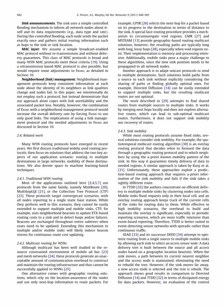
Nevertheless, these equations do not consider behaviorfor intermediate values. We, therefore, need to explorecomplexity in a network with constant jNj and different
density Y density Ydiameter M diameter M
complexitycomplexity
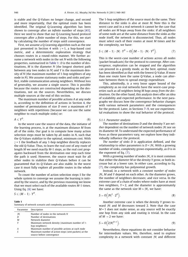
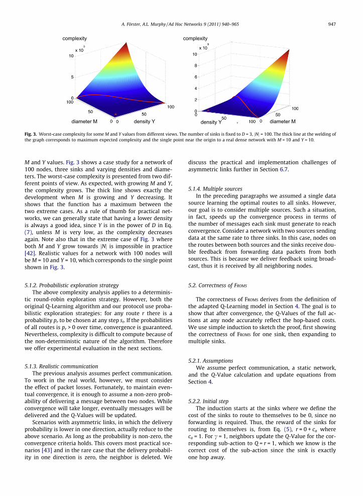
Fig. 3. Worst-case complexity for some M and Y values from different views. The number of sinks is fixed to D = 3, jNj = 100. The thick line at the welding ofthe graph corresponds to maximum expected complexity and the single point near the origin to a real dense network with M = 10 and Y = 10.
A. Förster, A.L. Murphy / Ad Hoc Networks 9 (2011) 940–965 947
M and Y values. Fig. 3 shows a case study for a network of100 nodes, three sinks and varying densities and diame-ters. The worst-case complexity is presented from two dif-ferent points of view. As expected, with growing M and Y,the complexity grows. The thick line shows exactly thedevelopment when M is growing and Y decreasing. Itshows that the function has a maximum between thetwo extreme cases. As a rule of thumb for practical net-works, we can generally state that having a lower densityis always a good idea, since Y is in the power of D in Eq.(7), unless M is very low, as the complexity decreasesagain. Note also that in the extreme case of Fig. 3 whereboth M and Y grow towards jNj is impossible in practice[42]. Realistic values for a network with 100 nodes willbe M = 10 and Y = 10, which corresponds to the single pointshown in Fig. 3.
5.1.2. Probabilistic exploration strategyThe above complexity analysis applies to a determinis-
tic round-robin exploration strategy. However, both theoriginal Q-Learning algorithm and our protocol use proba-bilistic exploration strategies: for any route r there is aprobability pr to be chosen at any step st. If the probabilitiesof all routes is pr > 0 over time, convergence is guaranteed.Nevertheless, complexity is difficult to compute because ofthe non-deterministic nature of the algorithm. Thereforewe offer experimental evaluation in the next sections.
5.1.3. Realistic communicationThe previous analysis assumes perfect communication.
To work in the real world, however, we must considerthe effect of packet losses. Fortunately, to maintain even-tual convergence, it is enough to assume a non-zero prob-ability of delivering a message between two nodes. Whileconvergence will take longer, eventually messages will bedelivered and the Q-Values will be updated.
Scenarios with asymmetric links, in which the deliveryprobability is lower in one direction, actually reduce to theabove scenario. As long as the probability is non-zero, theconvergence criteria holds. This covers most practical sce-narios [43] and in the rare case that the delivery probabil-ity in one direction is zero, the neighbor is deleted. We
discuss the practical and implementation challenges ofasymmetric links further in Section 6.7.
5.1.4. Multiple sourcesIn the preceding paragraphs we assumed a single data
source learning the optimal routes to all sinks. However,our goal is to consider multiple sources. Such a situation,in fact, speeds up the convergence process in terms ofthe number of messages each sink must generate to reachconvergence. Consider a network with two sources sendingdata at the same rate to three sinks. In this case, nodes onthe routes between both sources and the sinks receive dou-ble feedback from forwarding data packets from bothsources. This is because we deliver feedback using broad-cast, thus it is received by all neighboring nodes.
5.2. Correctness of FROMS
The correctness of FROMS derives from the definition ofthe adapted Q-Learning model in Section 4. The goal is toshow that after convergence, the Q-Values of the full ac-tions at any node accurately reflect the hop-based costs.We use simple induction to sketch the proof, first showingthe correctness of FROMS for one sink, then expanding tomultiple sinks.
5.2.1. AssumptionsWe assume perfect communication, a static network,
and the Q-Value calculation and update equations fromSection 4.
5.2.2. Initial stepThe induction starts at the sinks where we define the
cost of the sinks to route to themselves to be 0, since noforwarding is required. Thus, the reward of the sinks forrouting to themselves is, from Eq. (5), r = 0 + ca whereca = 1. For c = 1, neighbors update the Q-Value for the cor-responding sub-action to Q = r = 1, which we know is thecorrect cost of the sub-action since the sink is exactlyone hop away.
948 A. Förster, A.L. Murphy / Ad Hoc Networks 9 (2011) 940–965
5.2.3. Induction stepAssume that a node N (a sink or any other node) has a
correct estimation of the cost to the sink QN. Its reward isalways computed as r = minaQ(a) + ca, where mina Q(a) isnecessarily the above QN and ca = 1. When node N sendsits reward to its direct neighbors, they will update theircorresponding Q-Values for this node to QN + 1, which isthe correct estimation of the cost through node N, sincethey are exactly one hop further away from the sink thannode N. Thus, for any node N with correct estimations ofthe cost, its direct neighbors also receive correct cost esti-mations when a reward is sent.
With this, we have shown that FROMS converges to thecorrect hop-based costs for one sink in the network. In factwe know that FROMS is correct for one sink also because ofthe sink announcement propagation. During this network-wide broadcast, every node easily learns about the bestroutes in terms of hop count to a single sink. Thus, we haveboth a practical and a theoretical proof that FROMS con-verges to the correct costs for one sink. This is the begin-ning of the sketch of the second induction proof, whichshows that FROMS converges to the correct hop-based costsalso for more than one sink.
Assume a network with two sinks where the Q-Valuesto reach each sink individually have converged at all nodes(according to the above discussion). For simplicity we labelthe sinks A and B. The costs of B to reach itself is 0 and toreach sink A is a constant v = minaQB(a), which is the min-imum Q-Value for A at node B. Thus, the cost of reachingboth A and B at B is 0 + v and the reward of B isrB = (0 + v) + ca = v + 1. The direct neighbors of B will updatetheir own Q-Values to this reward value, which is the cor-rect cost: they need one hop to reach sink B and further vcosts to reach sink A. This trivially extends to the next-hops, as done above. It also intuitively extends to morethan 2 sinks.
5.2.4. OptimalityCombining the results for convergence of Section 5.1
with the correctness above shows that FROMS converges tothe correct hop-based costs of the routes after a finite num-ber of steps and thus finds the optimal route(s).
5.3. Memory and processing requirements
Two final aspects to consider are the memory and pro-cessing requirements at each network node.
Specifically, each node must store all locally availableroutes. Following Eq. (6), the expected storage is O(YD).The required processing includes selecting a route andupdating a Q-Value. The first function requires, in theworst case, to loop through all available routes to comparethem in terms of their costs and is thus bounded by O(YD).Updating a Q-Value is itself an atomic action: given the oldQ-Value and the reward, it calculates the new one. Assum-ing a data structure, organized by neighbor, this yields aworst case for searching O(Y + D).
Note again that the memory requirements for eachnode do not depend on the network size, but on the num-ber of neighbors. For networks with reasonable densities,the needed memory requirements are moderate, and for
high density scenarios we have developed special pruningtechniques, described in Section 6.4.
6. Protocol implementation details
The implementation outlined in this section is based onthe reinforcement learning model of Section 4 and intro-duces practical elements such as event-based processingand data structures tuned to the resource restricted envi-ronment of WSNs.
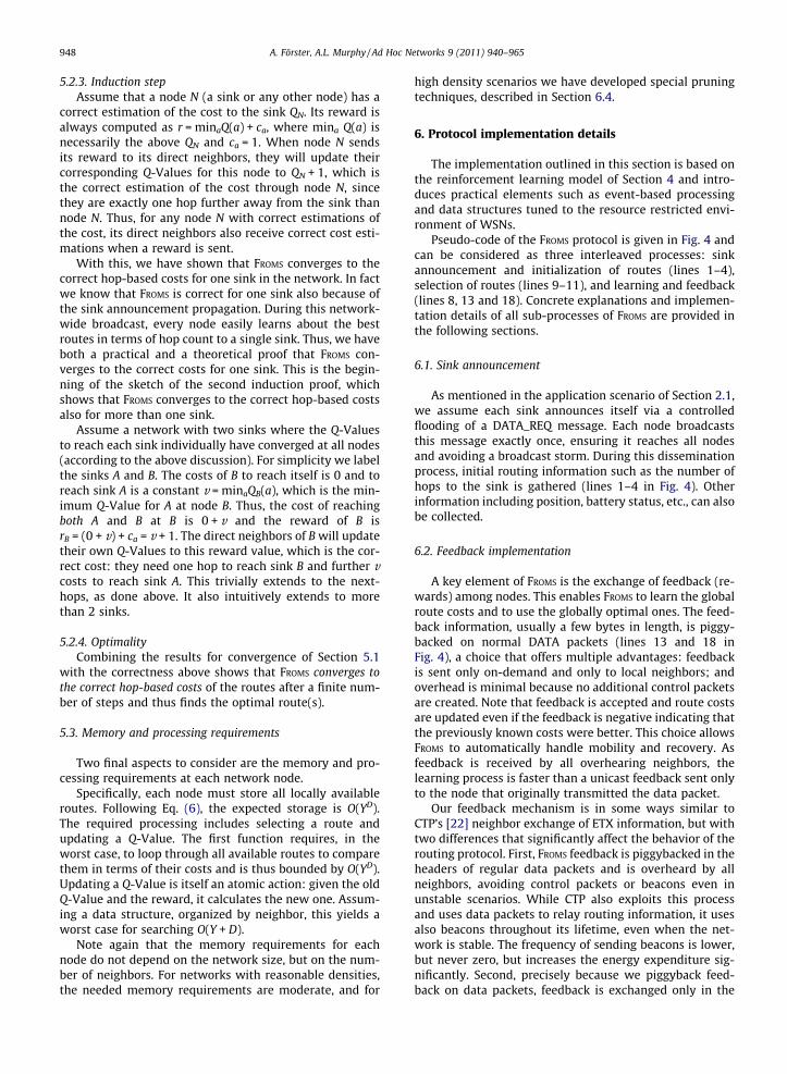
Pseudo-code of the FROMS protocol is given in Fig. 4 andcan be considered as three interleaved processes: sinkannouncement and initialization of routes (lines 1–4),selection of routes (lines 9–11), and learning and feedback(lines 8, 13 and 18). Concrete explanations and implemen-tation details of all sub-processes of FROMS are provided inthe following sections.
6.1. Sink announcement
As mentioned in the application scenario of Section 2.1,we assume each sink announces itself via a controlledflooding of a DATA_REQ message. Each node broadcaststhis message exactly once, ensuring it reaches all nodesand avoiding a broadcast storm. During this disseminationprocess, initial routing information such as the number ofhops to the sink is gathered (lines 1–4 in Fig. 4). Otherinformation including position, battery status, etc., can alsobe collected.
6.2. Feedback implementation
A key element of FROMS is the exchange of feedback (re-wards) among nodes. This enables FROMS to learn the globalroute costs and to use the globally optimal ones. The feed-back information, usually a few bytes in length, is piggy-backed on normal DATA packets (lines 13 and 18 inFig. 4), a choice that offers multiple advantages: feedbackis sent only on-demand and only to local neighbors; andoverhead is minimal because no additional control packetsare created. Note that feedback is accepted and route costsare updated even if the feedback is negative indicating thatthe previously known costs were better. This choice allowsFROMS to automatically handle mobility and recovery. Asfeedback is received by all overhearing neighbors, thelearning process is faster than a unicast feedback sent onlyto the node that originally transmitted the data packet.
Our feedback mechanism is in some ways similar toCTP’s [22] neighbor exchange of ETX information, but withtwo differences that significantly affect the behavior of therouting protocol. First, FROMS feedback is piggybacked in theheaders of regular data packets and is overheard by allneighbors, avoiding control packets or beacons even inunstable scenarios. While CTP also exploits this processand uses data packets to relay routing information, it usesalso beacons throughout its lifetime, even when the net-work is stable. The frequency of sending beacons is lower,but never zero, but increases the energy expenditure sig-nificantly. Second, precisely because we piggyback feed-back on data packets, feedback is exchanged only in the
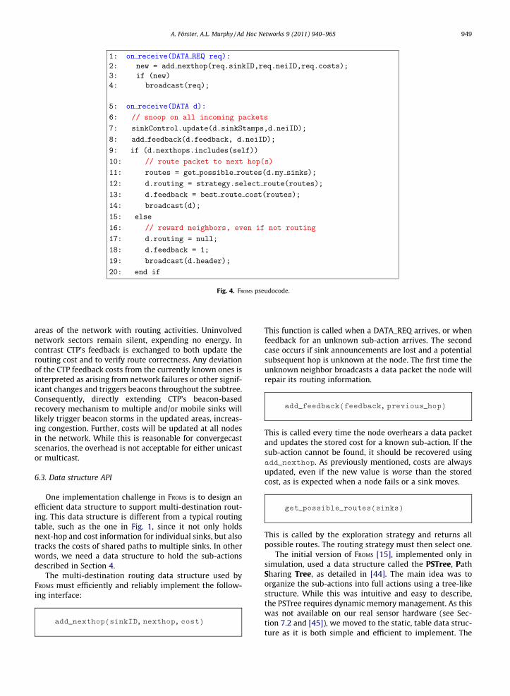
Fig. 4. FROMS pseudocode.
A. Förster, A.L. Murphy / Ad Hoc Networks 9 (2011) 940–965 949
areas of the network with routing activities. Uninvolvednetwork sectors remain silent, expending no energy. Incontrast CTP’s feedback is exchanged to both update therouting cost and to verify route correctness. Any deviationof the CTP feedback costs from the currently known ones isinterpreted as arising from network failures or other signif-icant changes and triggers beacons throughout the subtree.Consequently, directly extending CTP’s beacon-basedrecovery mechanism to multiple and/or mobile sinks willlikely trigger beacon storms in the updated areas, increas-ing congestion. Further, costs will be updated at all nodesin the network. While this is reasonable for convergecastscenarios, the overhead is not acceptable for either unicastor multicast.
6.3. Data structure API
One implementation challenge in FROMS is to design anefficient data structure to support multi-destination rout-ing. This data structure is different from a typical routingtable, such as the one in Fig. 1, since it not only holdsnext-hop and cost information for individual sinks, but alsotracks the costs of shared paths to multiple sinks. In otherwords, we need a data structure to hold the sub-actionsdescribed in Section 4.
The multi-destination routing data structure used byFROMS must efficiently and reliably implement the follow-ing interface:
add_nexthop(sinkID, nexthop, cost)
This function is called when a DATA_REQ arrives, or whenfeedback for an unknown sub-action arrives. The second
case occurs if sink announcements are lost and a potentialsubsequent hop is unknown at the node. The first time theunknown neighbor broadcasts a data packet the node willrepair its routing information.add_feedback(feedback, previous_hop)
This is called every time the node overhears a data packetand updates the stored cost for a known sub-action. If thesub-action cannot be found, it should be recovered usingadd_nexthop. As previously mentioned, costs are alwaysupdated, even if the new value is worse than the storedcost, as is expected when a node fails or a sink moves.
get_possible_routes(sinks)
This is called by the exploration strategy and returns allpossible routes. The routing strategy must then select one.
The initial version of FROMS [15], implemented only insimulation, used a data structure called the PSTree, PathSharing Tree, as detailed in [44]. The main idea was toorganize the sub-actions into full actions using a tree-likestructure. While this was intuitive and easy to describe,the PSTree requires dynamic memory management. As thiswas not available on our real sensor hardware (see Sec-tion 7.2 and [45]), we moved to the static, table data struc-ture as it is both simple and efficient to implement. The
950 A. Förster, A.L. Murphy / Ad Hoc Networks 9 (2011) 940–965
most recent implementation of FROMS, as presented here,leverages the so called Path Sharing Table or PSTable.Additional implementation details are available in [46].
6.4. Route storage reducing heuristics
As noted in Section 5, storage for routes grow exponen-tially with the number of sinks and polynomially with thenumber of neighbors. In practice this means that for largenumbers of sinks and neighbors we simply cannot store allroutes. The consequence is that we can no longer guaran-tee the optimality of learned routes. However, near-opti-mality can be preserved by wisely managing whichroutes to store and which to drop. In our previous workwe developed two pruning heuristics for the PSTree [15]and showed that the optimality of FROMS is only slightly af-fected, while the memory requirements are reduced signif-icantly. Interestingly, for the scenarios we evaluate inSection 9, we did not need to apply any pruning heuristics,as the full data structure fit comfortably in memory. Nev-ertheless, for scenarios with higher densities, the pruningheuristics are a valuable tool for reducing memoryconsumption.
6.5. Loop management
Because FROMS explores non-optimal routes to find theglobally best route, it may choose a route with a potentiallyunlimited length. In other words, it may be that a packettravels in a loop. We manage this problem by adding a sim-ple time-to-live (TTL) to all data packets. Implementationdetails are available in [46].
6.6. Node failure and mobility management
Our Q-Learning-based protocol has the innate ability tomanage changing network conditions. They simply appearas feedback and Q-Values are updated during the usuallearning process. However, practical challenges arise fromthe fact that increasing the costs of some route could eithermean a mobile sink is moving away or a sink is disconnect-ing. The first case is to be expected, however the secondwill cause packets to loop as they travel forever searchingfor non-existent sinks.
Properly managing mobility can be described in twosteps: identification of node failures and maintaining sinkfreshness. The first is used also for general neighbor failurerecognition and is accomplished by simply keeping a time-stamp at each node of when it last overheard a packet fromeach neighbor. If the timestamp becomes too old (a param-eter), then the neighbor is considered dead. A special casearises when the failing neighbor was a sink. In this case,the direct connection to the sink might have been lost,but the sink could be still alive and moving away. To iden-tify this situation we also keep a timestamp for each sink.Direct neighbors of the sink propagate the last time theyoverheard a packet from a sink to inform other nodes thatthe sink is still alive. Recall from Fig. 4, lines 18–19, thatsinks implicitly acknowledge the receipt of data packetswhen sending feedback.
With these two interleaved mechanisms, neighbor fail-ure detection and sink freshness tracking, each node as-sesses its neighborhood and can choose to use alternativeroutes, to re-learn optimal routes or to stop data deliveryto some sinks. For example, when a node, A, deletes aneighbor, D, because of D’s freshness value, A also deletesall routes that include D. However, alternate routes remainwith up-to-date Q-Values that can be selected by A imme-diately to route messages. Recall that each forwardedpacket contains the reward, equal to the current, bestavailable Q-Value. If the new, best Q-Value at A is the sameas before D’s deletion, A’s neighbors will not change theirQ-Values, even though the actual route has changed. Ifthe reward is worse (higher), A’s neighbors will updatetheir costs and the updated values will propagate on futurepackets until all nodes involved in routing update theircosts. Recall that only routing neighbors send feedback,thus limiting the scope of the updates to those on the pathas well as their neighbors that overhear the feedback.
It is worth noting that our failure recognition mecha-nism is not part of the Q-Learning protocol. It is simply asupporting module that sits beside the routing protocol.
6.7. Low quality and asymmetric links
Another major challenge for any routing protocol is tohandle low quality and asymmetric links. A recent studyhas shown that a relatively high percentage of links in realnetworks can be considered asymmetric or even unidirec-tional [43]. Various link quality management protocolshave been developed either as stand-alone solutions (e.g.,Arbutus [47]) or as part of other routing protocols (e.g.,CTP [22]). Their main goal is to evaluate the link qualityin both directions and provide this data to the higher layerprotocols, allowing them to avoid poor links.
Previous applications of RL to routing in WSNs (see Sec-tion 2.4) do not exploit such protocols, but instead have as-sumed perfect links while simultaneously arguing thatperfect links are not a requirement to find optimal paths.Nevertheless, the behavior of RL protocols in the face ofunreliable links has never been demonstrated. Therefore,for our evaluation of FROMS we show that with realistic,unreliable links and without a link management protocol,FROMS does perform properly, learning the best routes.
Despite our choice for this paper, a link quality protocolcould efficiently be integrated with FROMS, as our protocoloperates above the link layer and can utilize its informa-tion. This is discussed in depth in Section 10.
6.8. Exploration strategies
The exploration strategy controls how FROMS choosesbetween the available routes. It also controls the explora-tion/exploitation ratio, which is responsible for both find-ing the optimal route and minimizing routing costs. Inthis section, we concentrate on how the exploration strat-egy fits into the FROMS implementation rather than whatkind of exploration strategies are possible. Section 7.4.2discusses multiple strategies and evaluates them in thecontext of the application scenario.
A. Förster, A.L. Murphy / Ad Hoc Networks 9 (2011) 940–965 951
The exploration strategy is used at exactly one place inthe FROMS algorithm: when selecting a route. After line 11returns all possible routes that meet the requirements suchas decreasing the total hop count to the sinks, the explora-tion strategy selects one route to use in line 12. For exam-ple, a randomized strategy could decide with someprobability to select the optimal (lowest cost) route or torandomly select among all available routes. Another explo-ration strategy might decide to use the optimal route withsome probability or to round-robin among all availableroutes, etc.
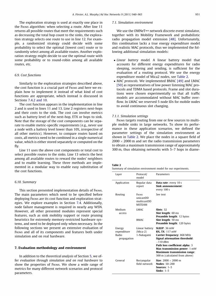
Table 2Summary of simulation environment model for our experiments.
6.9. Cost functions
Similarly to the exploration strategies described above,the cost function is a crucial part of FROMS and here we ex-plain how to implement it instead of what kind of costfunctions are appropriate, which instead is discussed inSections 7.4.2 and 10.
The cost function appears in the implementation in line2 and is used in lines 11 and 13. Line 2 registers next-hopsand their costs to the sink. The cost can involve metricssuch as battery level of the next-hop, ETX or hops to sink.Note that the storage of the cost components can be sepa-rate to enable metric-specific requirements (e.g., never usea node with a battery level lower than 10%, irrespective ofall other metrics). However, to compare routes based oncosts, all metrics need to be combined in a single numericalvalue, which is either stored separately or computed on thefly.
Line 11 uses the above cost components or total cost toselect possible routes to the sinks. Line 13 selects the bestamong all available routes to reward the nodes’ neighborsand to enable learning. These three methods are imple-mented in a modular way to enable easy substitution ofthe cost functions.
Layer Protocol/model
Parameters
Application Regular datareport
Data rate: every 10 sSink announcement:every 100 s
Routing FROMS See textunicastDDmulticastDDMSTEAM
Mediumaccess
LMAC Slots: 32Slot length: 60 msPreamble length: 12 bytes
BMAC Slot length: 50 msPreamble length: 120 bytes
Energy Linear battery SLEEP: 36 mWexpenditure (Mica-2) RX, TX: 117 mWRadio
propagation1-Nakagami Carrier frequency: 868 MHz
Signal attenuation threshold:
6.10. Summary
This section presented implementation details of FROMS.The main parameters which need to be specified beforedeploying FROMS are its cost function and exploration strat-egies. We explore examples in Section 7.4. Additionally,node failure management is required in nearly any WSN.However, all other presented modules represent specialfeatures, such as sink mobility support or route pruningheuristics for extremely memory-restricted hardware sys-tems, and need to be deployed only when necessary. In thefollowing sections we present an extensive evaluation ofFROMS and all of its components and features both undersimulation and on real hardware.
�110 dBmPath loss coefficient alpha: 3Max transmission power: 1 mWMaximum transmission range:300 m (calculated from above)
General Rectangularfield network
Size: 2000 � 2000 mNodes: 50–200Sources: 1–5Sinks: 1–5
7. Evaluation methodology and environment
In addition to the theoretical analysis of Section 5, we of-fer evaluation through simulation and on real hardware toshow the properties of FROMS. We show a wide range ofmetrics for many different network scenarios and protocolparameters.
7.1. Simulation environment
We use the OMNeT++ network discrete event simulator,together with its Mobility Framework and probabilisticradio propagation model extension [48]. Unfortunately,this combination lacks a true energy expenditure modeland realistic MAC protocols, thus we implemented the fol-lowing additional simulation models:
� Linear battery model. A linear battery model thataccounts for different energy expenditures for radiosleeping, receiving and sending, is sufficient for theevaluation of a routing protocol. We use the energyexpenditure model of Mica2 nodes, see Table 2.� MAC protocols. We implemented BMAC [49] and LMAC
[50] as representatives of low power listening MAC pro-tocols and TDMA based protocols. Frame and slot dura-tions were chosen experimentally so that all trafficmodels are accommodated without MAC buffer over-flow. In LMAC we reserved 5 node IDs for mobile nodesto avoid continuous slot changing.
7.1.1. Simulation settingsFROMS targets routing from one or few sources to multi-
ple mobile sinks in large networks. To show its perfor-mance in these application scenarios, we defined theparameter settings of the simulation environment asshown in Table 2. We place the nodes in a square field of2000 � 2000 m and set the radio transmission parametersto obtain a maximum transmission range of approximately300 m, thus obtaining networks with 5–7 hops in diame-
952 A. Förster, A.L. Murphy / Ad Hoc Networks 9 (2011) 940–965
ter. Note that the real transmission range varies signifi-cantly, as the radio propagation model is probabilistic-based.
We vary the number of nodes from 50 to 200, thus cov-ering medium to large networks. We vary the number ofsources from 1 to 5 or approximately 2–10% of the networknodes, which is reasonable for multicast scenarios. Wevary the number of sinks from 1 to 5. With these settings,we cover a large parameter space and the obtained resultspresent sufficient information to be able to predict thebehavior of the protocol on even larger scales.
In terms of data rate, we fix it to 1 packet every 10 s,which is reasonable for our low rate application scenarios.MAC protocol settings are chosen such that no congestionever occurs. We do not vary the data rate, as the maximumsupported throughout of the network depends more on theMAC protocol than the routing protocol. Nevertheless, weevaluate the processing time of FROMS in a testbed in Sec-tion 7.2. How data rate affects the mobility scenarios is dis-cussed in Section 8.3.
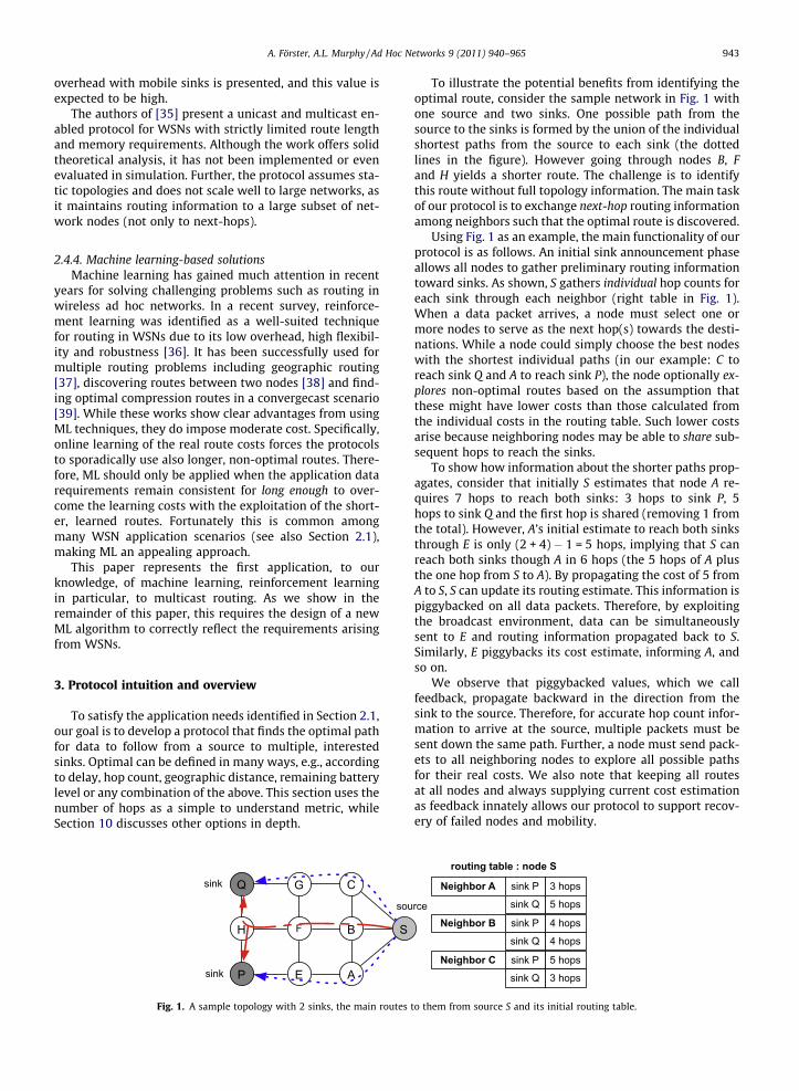
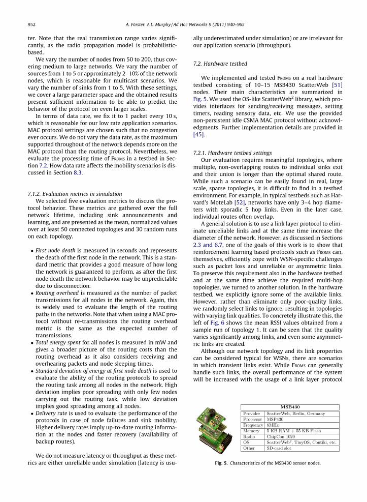
Fig. 5. Characteristics of the MSB430 sensor nodes.
7.1.2. Evaluation metrics in simulationWe selected five evaluation metrics to discuss the pro-
tocol behavior. These metrics are gathered over the fullnetwork lifetime, including sink announcements andlearning, and are presented as the mean, normalized valuesover at least 50 connected topologies and 30 random runson each topology.
� First node death is measured in seconds and representsthe death of the first node in the network. This is a stan-dard metric that provides a good measure of how longthe network is guaranteed to perform, as after the firstnode death the network behavior may be unpredictabledue to disconnection.� Routing overhead is measured as the number of packet
transmissions for all nodes in the network. Again, thisis widely used to evaluate the length of the routingpaths in the networks. Note that when using a MAC pro-tocol without re-transmissions the routing overheadmetric is the same as the expected number oftransmissions.� Total energy spent for all nodes is measured in mW and
gives a broader picture of the routing costs than therouting overhead as it also considers receiving andoverhearing packets and node sleeping times.� Standard deviation of energy at first node death is used to
evaluate the ability of the routing protocols to spreadthe routing task among all nodes in the network. Highdeviation implies poor spreading with only few nodescarrying out the routing task, while low deviationimplies good spreading among all nodes.� Delivery rate is used to evaluate the performance of the
protocols in case of node failures and sink mobility.Higher delivery rates imply up-to-date routing informa-tion at the nodes and faster recovery (availability ofbackup routes).
We do not measure latency or throughput as these met-rics are either unreliable under simulation (latency is usu-
ally underestimated under simulation) or are irrelevant forour application scenario (throughput).
7.2. Hardware testbed
We implemented and tested FROMS on a real hardwaretestbed consisting of 10–15 MSB430 ScatterWeb [51]nodes. Their main characteristics are summarized inFig. 5. We used the OS-like ScatterWeb2 library, which pro-vides interfaces for sending/receiving messages, settingtimers, reading sensory data, etc. We use the providednon-persistent idle CSMA MAC protocol without acknowl-edgments. Further implementation details are provided in[45].
7.2.1. Hardware testbed settingsOur evaluation requires meaningful topologies, where
multiple, non-overlapping routes to individual sinks exitand their union is longer than the optimal shared route.While such a scenario can be easily found in real, largescale, sparse topologies, it is difficult to find in a testbedenvironment. For example, in typical testbeds such as Har-vard’s MoteLab [52], networks have only 3–4 hop diame-ters with sporadic 5 hop links. Even in the later case,individual routes often overlap.
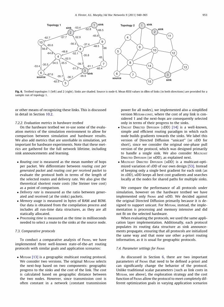
A general solution is to use a link layer protocol to elim-inate unreliable links and at the same time increase thediameter of the network. However, as discussed in Sections2.3 and 6.7, one of the goals of this work is to show thatreinforcement learning based protocols such as FROMS can,themselves, efficiently cope with WSN-specific challengessuch as packet loss and unreliable or asymmetric links.To preserve this requirement also in the hardware testbedand at the same time achieve the required multi-hoptopologies, we turned to another solution. In the hardwaretestbed, we explicitly ignore some of the available links.However, rather than eliminate only poor-quality links,we randomly select links to ignore, resulting in topologieswith varying link qualities. To concretely illustrate this, theleft of Fig. 6 shows the mean RSSI values obtained from asample run of topology 1. It can be seen that the qualityvaries significantly among links, and even some asymmet-ric links are created.
Although our network topology and its link propertiescan be considered typical for WSNs, there are scenariosin which transient links exist. While FROMS can generallyhandle such links, the overall performance of the systemwill be increased with the usage of a link layer protocol
1
7
3
4
8
9
5
2
6
10
-53.4 -52.8 -66.5
-65.6
-37.4-48.5
-66
-65
-61.1-60.4
-35.9-36.7
-35.5
-35.7
-34.5-35.5
-67.6
-62.5
-56.9
-53.4
-62.7 -57.7
-48.8-52.1
-65.6
-64.8-35.8
-39.7
-52.9
-56.3
-51.3
-52.5
source
1
2
3
8
9
7
4
6
5
14
12
15
13
10
11
source
Topology 1 Topology 2sink
sink
sink
sink
sink
sink
Fig. 6. Testbed topologies 1 (left) and 2 (right). Sinks are shaded. Source is node 6. Mean RSSI values in dBm of links (in both directions) are provided for asample run of topology 1.
A. Förster, A.L. Murphy / Ad Hoc Networks 9 (2011) 940–965 953
or other means of recognizing these links. This is discussedin detail in Section 10.2.
7.2.2. Evaluation metrics in hardware testbedOn the hardware testbed we re-use some of the evalu-
ation metrics of the simulation environment to allow forcomparison between simulation and hardware results.We also add metrics that are unreliable in simulation, yetimportant for hardware experiments. Note that these met-rics are gathered for the full network lifetime, includingsink announcements and learning.
� Routing cost is measured as the mean number of hopsper packet. We differentiate between routing cost pergenerated packet and routing cost per received packet toevaluate the protocol both in terms of the length ofthe selected routes and delivery rate. We also give thetheoretical shortest route costs (the Steiner tree cost)as a point of comparison.� Delivery rate is measured as the ratio between gener-
ated and received (at the sinks) packets.� Memory usage is measured in bytes of RAM and ROM.
Our data is obtained from the compilation process andincludes all run-time data structures, as they are allstatically allocated.� Processing time is measured as the time in milliseconds
needed to select a route to the sinks at the source node.
7.3. Comparative protocols
To conduct a comparative analysis of FROMS, we haveimplemented three well-known state-of-the-art routingprotocols with similar goals and application scenarios:
� MSTEAM [13] is a geographic multicast routing protocol.We consider two versions. The original MSTEAM selectsthe next-hop based on two components: geographicprogress to the sinks and the cost of the link. The costis calculated based on geographic distance betweenthe two nodes. However, since transmission cost isoften constant in a network (constant transmission
power for all nodes), we implemented also a simplifiedversion MSTEAM-CONST, where the cost of any link is con-sidered 1 and the next-hops are consequently selectedonly in terms of their progress to the sinks.� UNICAST DIRECTED DIFFUSION (UDD) [14] is a well-known,
simple and efficient routing paradigm in which eachnode builds gradients towards the sinks. We label thisversion of Directed Diffusion ‘‘unicast’’ (or UDD forshort), since we consider the original one-phase pullversion of the protocol, which was designed primarilyto handle a single sink. We also consider MULTICAST
DIRECTED DIFFUSION (or MDD), as explained next.� MULTICAST DIRECTED DIFFUSION (MDD) is a multicast-opti-
mized variation of UDD of our own design [53]. Insteadof keeping only a single best gradient for each sink (asin UDD), MDD keeps all best cost gradients and searcheslocally at the nodes for shared paths for multiple sinks.
We compare the performance of all protocols undersimulation, however on the hardware testbed we haveimplemented only FROMS and MDD. We decided againstthe original Directed Diffusion primarily because it is de-signed to support unicast. For MSTEAM, instead, the imple-mentation is processing and memory intensive and didnot fit on the selected hardware.
When evaluating the protocols, we used the same appli-cation layer implementation. Additionally, each protocolpopulates its routing data structure as sink announce-ments propagate, ensuring that all protocols are initializedthe same way and that none use other a-priori routinginformation, as it is usual for geographic protocols.
7.4. Parameter settings for FROMS
As discussed in Section 6, there are two importantparameters of FROMS that need to be defined a-priori andcan significantly change the behavior of the protocol.Unlike traditional scalar parameters (such as link costs inMSTEAM, see above), the exploration strategy and the costfunction of FROMS allow the protocol to meet completely dif-ferent optimization goals in varying application scenarios
954 A. Förster, A.L. Murphy / Ad Hoc Networks 9 (2011) 940–965
and to perform cross-layer optimization with other com-munication stack layers (see Section 10).
7.4.1. Cost function for mobile multicastRecall from Section 2.1 that our core scenarios require
multicast routing towards multiple, mobile sinks. We as-sume a retransmission-free MAC protocol and no neigh-borhood management protocol. Thus, the best costfunction to represent shortest paths is hop count. Note thatwith a retransmission-free MAC protocol there is exactlyone transmission per hop and therefore the number ofhops is equal to the number of expected transmissions(ETX). Thus, we use the hop-based cost functions pre-sented in Section 4.
7.4.2. Exploration strategy for mobile multicastThe exploration strategy must balance the potentially
large cost to explore routes against the exploitation ofthe best ones. Many different exploration strategies areavailable in the reinforcement learning community, eachsuitable to different settings. Unlike cost functions, whichcan be intuitively selected to meet some optimizationgoals (see the previous section), exploration strategies re-quire deeper evaluation, supported by experimentation.We use both sample runs and a large parameter spaceevaluation to compare several exploration strategies inthe mobile multicast scenario. These evaluations help toselect the best suited strategies for this specific scenario,and provide us with intuition for alternate applicationscenarios.
In our preliminary studies [15], we applied two differ-ent techniques for exploration: greedy and stochastic.The greedy strategy simply ignores exploration and alwayschooses between the best available routes. Stochasticexploration strategies on the other hand assign a probabil-ity to each of the routes, depending or not on their currentor initial Q-Values, and choose the routes accordingly.These exploration strategies showed good results, but are
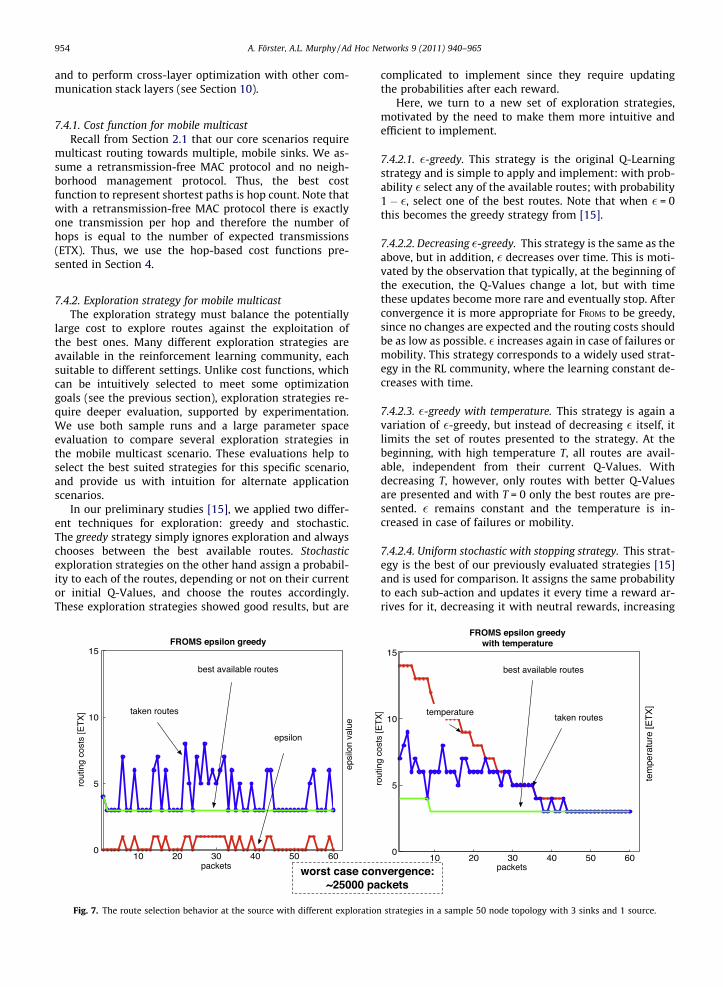
Fig. 7. The route selection behavior at the source with different exploratio
complicated to implement since they require updatingthe probabilities after each reward.
Here, we turn to a new set of exploration strategies,motivated by the need to make them more intuitive andefficient to implement.
7.4.2.1. �-greedy. This strategy is the original Q-Learningstrategy and is simple to apply and implement: with prob-ability � select any of the available routes; with probability1 � �, select one of the best routes. Note that when � = 0this becomes the greedy strategy from [15].
7.4.2.2. Decreasing �-greedy. This strategy is the same as theabove, but in addition, � decreases over time. This is moti-vated by the observation that typically, at the beginning ofthe execution, the Q-Values change a lot, but with timethese updates become more rare and eventually stop. Afterconvergence it is more appropriate for FROMS to be greedy,since no changes are expected and the routing costs shouldbe as low as possible. � increases again in case of failures ormobility. This strategy corresponds to a widely used strat-egy in the RL community, where the learning constant de-creases with time.
7.4.2.3. �-greedy with temperature. This strategy is again avariation of �-greedy, but instead of decreasing � itself, itlimits the set of routes presented to the strategy. At thebeginning, with high temperature T, all routes are avail-able, independent from their current Q-Values. Withdecreasing T, however, only routes with better Q-Valuesare presented and with T = 0 only the best routes are pre-sented. � remains constant and the temperature is in-creased in case of failures or mobility.
7.4.2.4. Uniform stochastic with stopping strategy. This strat-egy is the best of our previously evaluated strategies [15]and is used for comparison. It assigns the same probabilityto each sub-action and updates it every time a reward ar-rives for it, decreasing it with neutral rewards, increasing
n strategies in a sample 50 node topology with 3 sinks and 1 source.
A. Förster, A.L. Murphy / Ad Hoc Networks 9 (2011) 940–965 955
it with negative rewards, and leaving it the same with po-sitive rewards. It stops exploration completely after somenumber of continuous neutral rewards to the node andstarts it again with negative/positive rewards.
Fig. 7 presents sample runs for �-greedy and �-greedywith temperature to further explain their behavior. It canbe seen for both strategies, that the best routes are found
0 1 2 3 4 5 6
1.002
1.
0.998
0.996
0.994
0.992
0.99
number of sinks
time
(nor
mal
ized
)
First node death comparison, BMAC
FROMS decr 05FROMS greedy 01FROMS greedy 03FROMS tempFROMS uniform
0 1 2 3 4 5 60.96
0.965
0.97
0.975
0.98
0.985
0.99
0.995
1
1.005
1.01
number of sources
time
(nor
mal
ized
)
First node death comparison, BMAC
FROMS decr 05FROMS greedy 01FROMS greedy 03FROMS tempFROMS uniform
50 75 100 150 175 2000.975
0.98
0.985
0.99
0.995
1
number of nodes
time
(nor
mal
ized
)
First node death comparison, BMAC
FROMS decr 05FROMS greedy 01FROMS greedy 03FROMS tempFROMS uniform
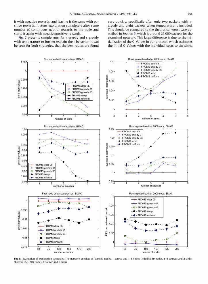
Fig. 8. Evaluation of exploration strategies. The network consists of (top) 50 no(bottom) 50–200 nodes, 1 source and 2 sinks.
very quickly, specifically after only two packets with �-greedy and eight packets when temperature is included.This should be compared to the theoretical worst case de-scribed in Section 5, which is around 25,000 packets for theexamined network. This large difference is due to the ini-tialization of the Q-Values in our protocol, which estimatesthe initial Q-Values with the individual costs to the sinks.
0 1 2 3 4 5 6
1
1.02
1.04
1.06
1.08
1.1
number of sinks
Routing overhead after 2000 secs, BMAC
FROMS decr 05FROMS greedy 01FROMS greedy 03FROMS tempFROMS uniform
over
head
(nor
mal
ized
)
0 1 2 3 4 5 60.95
1
1.05
1.1
1.15
1.2
1.25
number of sources
Routing overhead for 2000 secs, BMAC
FROMS decr 05FROMS greedy 01FROMS greedy 03FROMS tempFROMS uniform
over
head
(nor
mal
ized
)
50 75 100 150 175 200
1
1.02
1.04
1.06
1.08
1.1
number of nodes
ETX
per d
eliv
ered
pac
ket
Routing overhead for 2000 secs, BMAC
FROMS decr 05FROMS greedy 01FROMS greedy 03FROMS tempFROMS uniform
des, 1 source and 1–5 sinks; (middle) 50 nodes, 1–5 sources and 2 sinks;
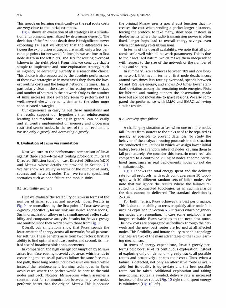
956 A. Förster, A.L. Murphy / Ad Hoc Networks 9 (2011) 940–965
This speeds up learning significantly as the real route costsare very close to the initial estimates.
Fig. 8 shows an evaluation of all strategies in a simula-tion environment, normalized by decreasing �-greedy. Thedeviation of the first node death time is insignificant, neverexceeding 1%. First we observe that the differences be-tween the exploration strategies are small: only a few per-centage points for network lifetime (shown as time to firstnode death in the left plots) and 10% for routing overhead(shown in the right plots). From this, we conclude that asimple to implement and tune exploration strategy suchas �-greedy or decreasing �-greedy is a reasonable choice.This choice is also supported by the absolute performanceof these two strategies as in most cases they show the low-est routing costs and the longest network lifetimes. This isparticularly clear in the cases of increasing network sizesand number of sources in the network. Only as the numberof sinks increases does �-greedy seem to perform not aswell, nevertheless, it remains similar to the other moresophisticated strategies.
Our experience in carrying out these simulations andthe results support our hypothesis that reinforcementlearning and machine learning in general can be easilyand efficiently implemented on memory and processingrestricted sensor nodes. In the rest of the our evaluationswe use only �-greedy and decreasing �-greedy.
8. Evaluation of FROMS via simulation
Next we turn to the performance comparison of FROMS
against three state-of-the-art routing protocols: multicastDirected Diffusion (MDD), unicast Directed Diffusion (UDD)and MSTEAM, whose details are provided in Section 7.3.We fist show scalability in terms of the number of sinks,sources and network nodes. Then we turn to specializedscenarios such as node failure and mobile sinks.
8.1. Scalability analysis
First we evaluate the scalability of FROMS in terms of thenumber of sinks, sources and network nodes. Results inFig. 9 are normalized by the first point of FROMS decreasing�-greedy (specifically for one sink, one source, and 50 nodes).Such normalization allows us to simultaneously offer scala-bility and comparative analysis. Results for FROMS �-greedyare omitted since they overlap with those from Fig. 8.
Overall, our simulations show that FROMS spends theleast amount of energy across all networks for all parame-ter settings. These benefits arise from two factors: first, itsability to find optimal multicast routes and second, its lim-ited use of broadcast sink announcements.
In comparison, the high energy consumption by MSTEAM
arises from face-routing to avoid void areas, which tends tocreate long routes. As all packets follow the same face-rou-ted path, these long routes incur excessive overhead, whileinstead the reinforcement learning techniques in FROMS
avoid cases where the packet would be sent to the voidnodes and back. Notably, MSTEAM-CONST which assumes aconstant cost for communication between any two nodesperforms better than the original MSTEAM. This is because
the original MSTEAM uses a special cost function that in-creases the cost when sending a packet longer distances,forcing the protocol to take many, short hops. Instead, indeployments where the radio transmission power is oftenfixed, longer hops lead to overall energy savings, evenwhen considering re-transmissions.
In terms of the overall scalability, we note that all pro-tocols scale well with all network parameters. This is dueto their localized nature, which makes them independentwith respect to the size of the network or the number ofsinks and sources.
In summary, FROMS achieves between 10% and 22% long-er network lifetimes in terms of first node death, incursaround two times less routing overhead, spends between5% and 15% less energy, and shows 2–3 times lower stan-dard deviation among the remaining node energies. Plotsfor lifetime and routing support the observations madehere but are not shown due to space reasons. We also com-pared the performance with LMAC and BMAC, achievingsimilar results.
8.2. Recovery after failure
A challenging situation arises when one or more nodesfail. Routes from sources to the sinks need to be repaired asquickly as possible to prevent data loss. To study thebehavior of the analyzed routing protocols in this situationwe conducted simulations in which we assign lower initialbattery levels to a random subset of nodes, causing them tofail prematurely. We consider this scenario more realisticcompared to a controlled killing of nodes at some prede-fined time, since in real deployments nodes do not diesimultaneously.
Fig. 10 shows the total energy spent and the deliveryrate for all protocols, with each point averaging 50 topol-ogies with 30 different random sets of failed nodes. Wenote that we ignore the results where the failures re-sulted in disconnected topologies, as in such scenariosthe data cannot be delivered. The standard deviation is2–3.3%.
For both metrics, FROMS achieves the best performance.This is due to its ability to recover quickly after node fail-ures. As explained in Section 6.6, it tracks which neighbor-ing nodes are responding. In case some neighbor is nolonger reachable, FROMS switches to the next best route.The new costs are propagated as feedback through the net-work and the new, best routes are learned at all affectednodes. This flexibility and innate ability to handle topologychanges are two of the main advantages of the FROMS learn-ing mechanism.
In terms of energy expenditure, FROMS �-greedy per-forms best because of its continuous exploration. Insteadof exploring only on demand, �-greedy tracks all possibleroutes and proactively updates their costs. Thus, when afailure is detected, not only an alternative route is avail-able, but its quality is up-to-date and the best possibleroute can be taken. Additional exploration and takingnon-optimal routes is avoided, delivery rate is increasedbecause of shorter routes (Fig. 10 right), and spent energyis minimized (Fig. 10 left).
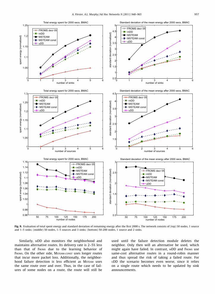
0 1 2 3 4 5 61
1.05
1.1
1.15
1.2
1.25
number of sinks
FROMS decr 05mDDMSTEAMMSTEAM constuDD
spen
t ene
rgy
(nor
mal
ized
)Total energy spent for 2000 secs, BMAC
0 1 2 3 4 5 60.5
1
1.5
2
2.5
3
3.5
4
4.5
5
number of sinks
Standard deviation of the mean energy after 2000 secs, BMAC
FROMS decr 05mDDMSTEAMMSTEAM constuDD
stan
dard
dev
iatio
n (n
orm
aliz
ed)
0 1 2 3 4 5 61
1.05
1.1
1.15
1.2
1.25
1.3
number of sources
FROMS decr 05mDDMSTEAMMSTEAM constuDD
spen
t ene
rgy
(nor
mal
ized
)
Total energy spent for 2000 secs, BMAC
0 1 2 3 4 5 61
1.5
2
2.5
3
3.5
4
4.5
number of sources
Standard deviation of the mean energy after 2000 secs, BMAC
FROMS decr 05mDDMSTEAMMSTEAM constuDD
stan
dard
dev
iatio
n (n
orm
aliz
ed)
50 75 100 125 150 175 2000.96
0.98
1
1.02
1.04
1.06
1.08
1.1
1.12
1.14
1.16
number of nodes
FROMS decr 05mDDMSTEAMMSTEAM constuDD
spen
t ene
rgy
(nor
mal
ized
)
Total energy spent for 2000 secs, BMAC
50 75 100 125 150 175 2000.5
1
1.5
2
2.5
3
number of nodes
Standard deviation of the mean energy after 2000 secs, BMAC
FROMS decr 05mDDMSTEAMMSTEAM constuDD
stan
dard
dev
iatio
n (n
orm
aliz
ed)
Fig. 9. Evaluation of total spent energy and standard deviation of remaining energy after the first 2000 s. The network consists of (top) 50 nodes, 1 sourceand 1–5 sinks; (middle) 50 nodes, 1–5 sources and 3 sinks; (bottom) 50-200 nodes, 1 source and 2 sinks.
A. Förster, A.L. Murphy / Ad Hoc Networks 9 (2011) 940–965 957
Similarly, MDD also monitors the neighborhood andmaintains alternative routes. Its delivery rate is 2–5% lessthan that of FROMS due to the learning behavior ofFROMS. On the other side, MSTEAM-CONST uses longer routesthat incur more packet loss. Additionally, the neighbor-hood failure detection is less efficient as MSTEAM usesthe same route over and over. Thus, in the case of fail-ures of some nodes on a route, the route will still be
used until the failure detection module deletes theneighbor. Only then will an alternative be used, whichmight again have failed. In contrast, MDD and FROMS usesame-cost alternative routes in a round-robin mannerand thus spread the risk of taking a failed route. ForUDD the scenario becomes even worse, since it relieson a single route which needs to be updated by sinkannouncements.
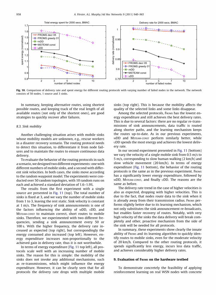
2 3 5 7 100.8
0.9
1
1.1
1.2
1.3
1.4
1.5
1.6
1.7
number of failed nodes
FROMS decr 05FROMS greedy 01mDDMSTEAM constuDD
spen
t ene
rgy
(nor
mal
ized
)Total energy spent for 2000 secs, BMAC
2 3 5 7 100.75
0.8
0.85
0.9
0.95
1
number of failed nodes
Delivery rate for 2000 secs, BMAC
FROMS decr 05FROMS greedy 01mDDMSTEAM constuDD
deliv
ery
rate
(nor
mal
ized
)
Fig. 10. Comparison of delivery rate and spent energy for different routing protocols with varying number of failed nodes in the network. The networkconsists of 50 nodes, 1 source and 3 sinks.
958 A. Förster, A.L. Murphy / Ad Hoc Networks 9 (2011) 940–965
In summary, keeping alternative routes, using shortestpossible routes, and keeping track of the real length of allavailable routes (not only of the shortest ones), are goodstrategies to quickly recover after failures.
8.3. Sink mobility
Another challenging situation arises with mobile sinkswhose mobility models are unknown, e.g., rescue workersin a disaster recovery scenario. The routing protocol needsto detect this situation, to differentiate it from node fail-ures and to maintain the routes to ensure continuous datadelivery.
To evaluate the behavior of the routing protocols in sucha scenario, we designed two different experiments: one withdifferent numbers of mobile sinks, and a second with differ-ent sink velocities. In both cases, the sinks move accordingto the random waypoint model. The experiments were con-ducted over 50 random topologies, with 10 random runs oneach and achieved a standard deviation of 1.6–1.9%.
The results from the first experiment with a singlesource are presented in Fig. 11 (top). The total number ofsinks is fixed at 3, and we vary the number of mobile sinksfrom 1 to 3, leaving the rest static. Sink velocity is constantat 1 m/s. The frequency of sink announcements is one ofthe factors influencing the ability of MDD, UDD, andMSTEAM-CONST to maintain correct, short routes to mobilesinks. Therefore, we experimented with two different fre-quencies, sending a sink announcement every 50 or100 s. With the higher frequency, the delivery rate in-creased as expected (top right), but correspondingly theenergy consumed also increased (top left). However, en-ergy expenditure increases non-proportionally to theachieved gain in delivery rate, thus it is not worthwhile.
In terms of energy expenditure (Fig. 11 top left), all pro-tocols scale well with an increasing number of mobilesinks. The reason for this is simple: the mobility of thesinks does not invoke any additional mechanisms, suchas re-transmissions, which might influence the energyexpenditure. However, it can be clearly seen that for allprotocols the delivery rate drops with multiple mobile
sinks (top right). This is because the mobility affects thequality of the selected links and some links disappear.
Among the selected protocols, FROMS has the lowest en-ergy expenditure and still achieves the best delivery rates.This is due to several factors: there are no regular re-trans-missions of sink announcements, data traffic is routedalong shorter paths, and the learning mechanism keepsthe routes up-to-date. As in our previous experiments,MDD and MSTEAM-CONST perform similarly better, whileUDD spends the most energy and achieves the lowest deliv-ery rate.
In our second experiment presented in Fig. 11 (bottom)we vary the velocity of a single mobile sink from 0.5 m/s to5 m/s, corresponding to slow human walking (2 km/h) andslow vehicle movement (20 km/h). In terms of energyexpenditure (Fig. 11 bottom), the behavior of the routingprotocols is the same as in the previous experiment. FROMS
has a significantly lower energy expenditure, followed byMDD, MSTEAM-CONST, and finally UDD. The reasons are thesame as before.
The delivery rate trend in the case of higher velocities isalso as expected, dropping with higher velocities. This isdue to the fact, that nodes route data to the sink when itis already away from their transmission radius. FROMS per-forms slightly better due to its learning mechanism, whichnot only substitutes the sink announcement re-broadcasts,but enables faster recovery of routes. Notably, with veryhigh velocity of the sinks the data delivery will break com-pletely and other, proactive mechanism from the side ofthe sink will be needed for all protocols.
In summary, these experiments show clearly the innateability of FROMS and its learning algorithm to quickly iden-tify routes to mobile sinks, even for the moderate velocityof 20 km/h. Compared to the other routing protocols, itspends significantly less energy, incurs less data traffic,and achieves considerably higher delivery rates.
9. Evaluation of FROMS on the hardware testbed
To demonstrate concretely the feasibility of applyingreinforcement learning on real WSN nodes with concrete
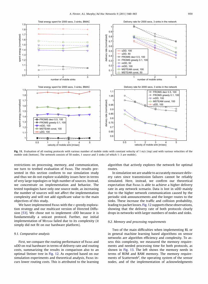
1 2 30.9
1
1.1
1.2
1.3
1.4
1.5
1.6
1.7
1.8
1.9
number of mobile sinks
Total energy spent for 2000 secs, 3 sinks, BMACsp
ent e
nerg
y (n
orm
aliz
ed)
1 2 30
0.1
0.2
0.3
0.4
0.5
0.6
0.7
0.8
0.9
1
number of mobile sinks
Delivery rate for 2000 secs, 3 sinks in the network
uDD, 100uDD, 50FROMS decr 0.5, 100FROMS greedy 0.1, 100mDD, 50mDD, 100MSTEAM const, 100MSTEAM const, 50
deliv
ery
rate
(nor
mal
ized
)
0.5 1 2 3 4 5
1
1.1
1.2
1.3
1.4
1.5
1.6
1.7
1.8
1.9
velocity of mobile sink [m/sec]
FROMS decr 0.5, 100FROMS greedy 0.1, 100mDD, 100MSTEAM const, 100uDD, 100
Total energy spent for 2000 secs, 3 sinks, BMAC
spen
t ene
rgy
(nor
mal
ized
)
0.5 1 2 3 4 5
0.6
0.65
0.7
0.75
0.8
0.85
0.9
0.95
1
1.05
1.1
velocity of mobile sink [m/sec]
Delivery rate for 2000 secs, 3 sinks in the network
FROMS decr 0.5, 100FROMS greedy 0.1, 100mDD, 100MSTEAM const, 100uDD, 100
deliv
ery
rate
(nor
mal
ized
)
Fig. 11. Evaluation of all routing protocols with various number of mobile sinks with constant velocity of 1 m/s (top) and with various velocities of themobile sink (bottom). The network consists of 50 nodes, 1 source and 3 sinks (of which 1–3 are mobile).
A. Förster, A.L. Murphy / Ad Hoc Networks 9 (2011) 940–965 959
restrictions on processing, memory, and communication,we turn to testbed evaluation of FROMS. The results pre-sented in this section conform to our simulation studyand thus we do not explore scalability issues here in termsof very large topologies or high number of sources. Instead,we concentrate on implementation and behavior. Thetested topologies have only one source node, as increasingthe number of sources will not affect the implementationcomplexity and will not add significant value to the mainobjectives of this study.
We have implemented FROMS with the �-greedy explora-tion strategy and our multicast version of Directed Diffu-sion [53]. We chose not to implement UDD because it isfundamentally a unicast protocol. Further, our initialimplementation of MSTEAM failed due to its complexity (itsimply did not fit on our hardware platform).
9.1. Comparative analysis
First, we compare the routing performance of FROMS andMDD on real hardware in terms of delivery rate and routingcosts, summarizing the results in comparison also to anoptimal Steiner tree in Fig. 12. As expected based on oursimulation experiments and theoretical analysis, FROMS in-curs lower routing costs. This is attributed to the learning
algorithm that actively explores the network for optimalroutes.
In simulation we are unable to accurately measure deliv-ery rates since transmission failures cannot be reliablysimulated. Here, instead, we confirm our theoreticalexpectation that FROMS is able to achieve a higher deliveryrate in any network scenario. Data is lost in MDD mainlydue to the higher network communication caused by theperiodic sink announcements and the longer routes to thesinks. These increase the traffic and collision probability,leading to packet losses. Fig. 12 supports these observations,showing that the delivery rate of both protocols clearlydrops in networks with larger numbers of nodes and sinks.
9.2. Memory and processing requirements
Two of the main difficulties when implementing RL orin general machine learning based algorithms on sensornetworks are algorithm efficiency and complexity. To as-sess this complexity, we measured the memory require-ments and needed processing time for both protocols, asshown in Fig. 13. The left shows the memory needs interms of ROM and RAM memory. The memory require-ments of Scatterweb2, the operating system of the sensornodes, and of the implementation of acknowledgments
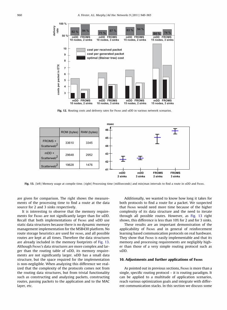
82 % 94 %
mDD FROMS
50 %
100 %
deliv
ery
rate
cost
s pe
r pac
ket i
n ET
X
6
3
4
5
7
10 nodes, 2 sinksmDD FROMS
10 nodes, 3 sinksmDD FROMS
15 nodes, 2 sinksmDD FROMS
15 nodes, 3 sinks
71 %87 % 83 % 94 %
64 % 74 %
cost per received packetcost per generated packetoptimal (Steiner tree) cost
9
8
10
mDD FROMS10 nodes, 2 sinks
mDD FROMS10 nodes, 3 sinks
mDD FROMS15 nodes, 2 sinks
mDD FROMS15 nodes, 3 sinks
Fig. 12. Routing costs and delivery rates for FROMS and MDD in various network scenarios.
41
42
43
44
45
msec
mDD2 sinks
mDD3 sinks
FROMS2 sinks
FROMS3 sinks
46
FROMS + Scatterweb2
mDD + Scatterweb2
Scatterweb2
33610
29648
19628
ROM (bytes)
3345
2952
1476
RAM (bytes)
Fig. 13. (left) Memory usage at compile time. (right) Processing time (milliseconds) and min/max intervals to find a route in MDD and FROMS.
960 A. Förster, A.L. Murphy / Ad Hoc Networks 9 (2011) 940–965
are given for comparison. The right shows the measure-ments of the processing time to find a route at the datasource for 2 and 3 sinks respectively.
It is interesting to observe that the memory require-ments for FROMS are not significantly larger than for MDD.Recall that both implementations of FROMS and MDD usestatic data structures because there is no dynamic memorymanagement implementation for the MSB430 platform. Noroute storage heuristics are used for FROMS, and all possibleroutes are kept at all times. Therefore the data structuresare already included in the memory footprints of Fig. 13.Although FROMS’s data structures are more complex and lar-ger than the routing table of MDD, its memory require-ments are not significantly larger. MDD has a small datastructure, but the space required for the implementationis non-negligible. When analyzing this difference we real-ized that the complexity of the protocols comes not fromthe routing data structures, but from trivial functionalitysuch as constructing and analyzing packets, constructingroutes, passing packets to the application and to the MAClayer, etc.
Additionally, we wanted to know how long it takes forboth protocols to find a route for a packet. We suspectedthat FROMS would need more time because of the highercomplexity of its data structure and the need to iteratethrough all possible routes. However, as Fig. 13 rightshows, this difference is less than 10% for 2 and for 3 sinks.
These results are an important demonstration of theapplicability of FROMS and in general of reinforcementlearning based communication protocols on real hardware.They show that FROMS is easily implementable and that itsmemory and processing requirements are negligibly high-er than those of a very simple routing protocol such asMDD.
10. Adjustments and further applications of FROMS
As pointed out in previous sections, FROMS is more than asingle, specific routing protocol – it is routing paradigm. Itcan be applied to a multitude of application scenarios,reach various optimization goals and integrate with differ-ent communication stacks. In this section we discuss some
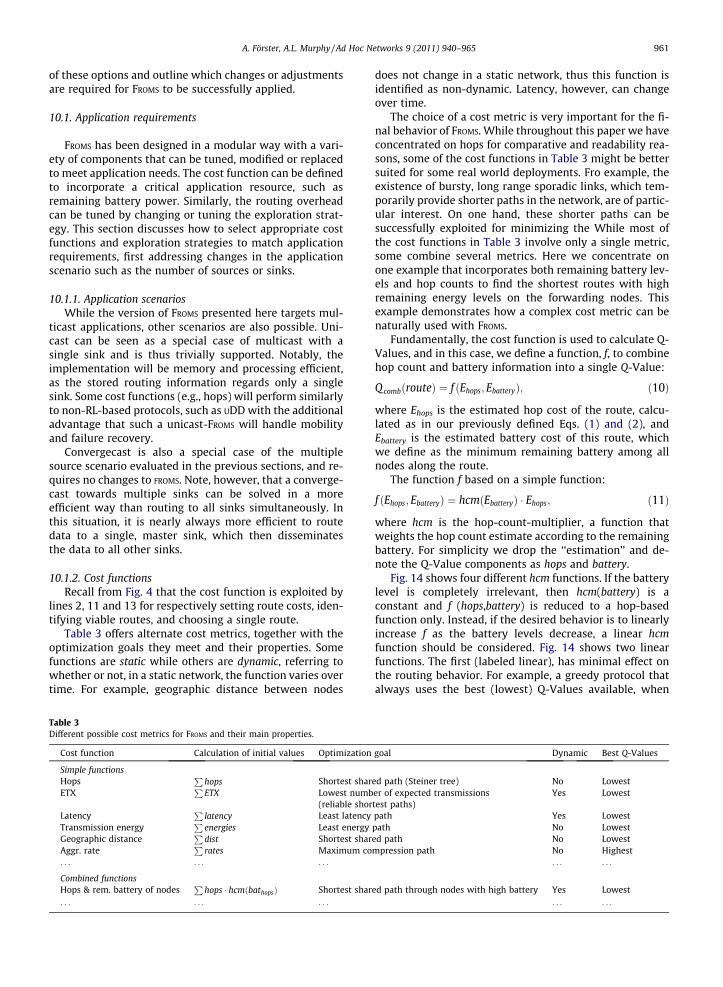
A. Förster, A.L. Murphy / Ad Hoc Networks 9 (2011) 940–965 961
of these options and outline which changes or adjustmentsare required for FROMS to be successfully applied.
10.1. Application requirements
FROMS has been designed in a modular way with a vari-ety of components that can be tuned, modified or replacedto meet application needs. The cost function can be definedto incorporate a critical application resource, such asremaining battery power. Similarly, the routing overheadcan be tuned by changing or tuning the exploration strat-egy. This section discusses how to select appropriate costfunctions and exploration strategies to match applicationrequirements, first addressing changes in the applicationscenario such as the number of sources or sinks.
10.1.1. Application scenariosWhile the version of FROMS presented here targets mul-
ticast applications, other scenarios are also possible. Uni-cast can be seen as a special case of multicast with asingle sink and is thus trivially supported. Notably, theimplementation will be memory and processing efficient,as the stored routing information regards only a singlesink. Some cost functions (e.g., hops) will perform similarlyto non-RL-based protocols, such as UDD with the additionaladvantage that such a unicast-FROMS will handle mobilityand failure recovery.
Convergecast is also a special case of the multiplesource scenario evaluated in the previous sections, and re-quires no changes to FROMS. Note, however, that a converge-cast towards multiple sinks can be solved in a moreefficient way than routing to all sinks simultaneously. Inthis situation, it is nearly always more efficient to routedata to a single, master sink, which then disseminatesthe data to all other sinks.
10.1.2. Cost functionsRecall from Fig. 4 that the cost function is exploited by
lines 2, 11 and 13 for respectively setting route costs, iden-tifying viable routes, and choosing a single route.
Table 3 offers alternate cost metrics, together with theoptimization goals they meet and their properties. Somefunctions are static while others are dynamic, referring towhether or not, in a static network, the function varies overtime. For example, geographic distance between nodes
Table 3Different possible cost metrics for FROMS and their main properties.
Cost function Calculation of initial values Optimization
Simple functionsHops
Phops Shortest shar
ETXP
ETX Lowest numb(reliable shor
LatencyP
latency Least latencyTransmission energy
Penergies Least energy
Geographic distanceP
dist Shortest sharAggr. rate
Prates Maximum co
. . . . . . . . .
Combined functionsHops & rem. battery of nodes
Phops � hcmðbathopsÞ Shortest shar
. . . . . . . . .
does not change in a static network, thus this function isidentified as non-dynamic. Latency, however, can changeover time.
The choice of a cost metric is very important for the fi-nal behavior of FROMS. While throughout this paper we haveconcentrated on hops for comparative and readability rea-sons, some of the cost functions in Table 3 might be bettersuited for some real world deployments. Fro example, theexistence of bursty, long range sporadic links, which tem-porarily provide shorter paths in the network, are of partic-ular interest. On one hand, these shorter paths can besuccessfully exploited for minimizing the While most ofthe cost functions in Table 3 involve only a single metric,some combine several metrics. Here we concentrate onone example that incorporates both remaining battery lev-els and hop counts to find the shortest routes with highremaining energy levels on the forwarding nodes. Thisexample demonstrates how a complex cost metric can benaturally used with FROMS.
Fundamentally, the cost function is used to calculate Q-Values, and in this case, we define a function, f, to combinehop count and battery information into a single Q-Value:
Q combðrouteÞ ¼ f ðEhops; EbatteryÞ; ð10Þ
where Ehops is the estimated hop cost of the route, calcu-lated as in our previously defined Eqs. (1) and (2), andEbattery is the estimated battery cost of this route, whichwe define as the minimum remaining battery among allnodes along the route.
The function f based on a simple function:
f ðEhops; EbatteryÞ ¼ hcmðEbatteryÞ � Ehops; ð11Þ
where hcm is the hop-count-multiplier, a function thatweights the hop count estimate according to the remainingbattery. For simplicity we drop the ‘‘estimation’’ and de-note the Q-Value components as hops and battery.
Fig. 14 shows four different hcm functions. If the batterylevel is completely irrelevant, then hcm(battery) is aconstant and f (hops,battery) is reduced to a hop-basedfunction only. Instead, if the desired behavior is to linearlyincrease f as the battery levels decrease, a linear hcmfunction should be considered. Fig. 14 shows two linearfunctions. The first (labeled linear), has minimal effect onthe routing behavior. For example, a greedy protocol thatalways uses the best (lowest) Q-Values available, when
goal Dynamic Best Q-Values
ed path (Steiner tree) No Lowester of expected transmissionstest paths)
Yes Lowest
path Yes Lowestpath No Lowested path No Lowestmpression path No Highest
. . . . . .
ed path through nodes with high battery Yes Lowest. . . . . .
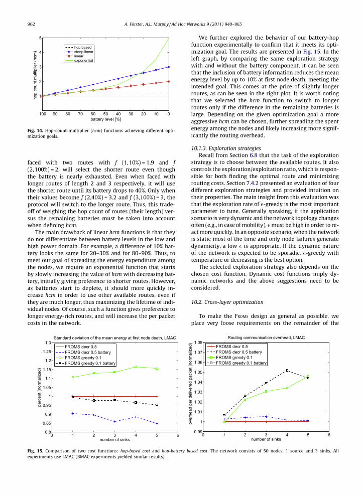
100 90 80 70 60 50 40 30 20 10 0
1
2
3
4
5
battery level [%]
hop
coun
t mul
tiplie
r (hc
m)
hop basedsteep linearlinearexponential
Fig. 14. Hop-count-multiplier (hcm) functions achieving different opti-mization goals.
962 A. Förster, A.L. Murphy / Ad Hoc Networks 9 (2011) 940–965
faced with two routes with f (1,10%) = 1.9 and f(2,100%) = 2, will select the shorter route even thoughthe battery is nearly exhausted. Even when faced withlonger routes of length 2 and 3 respectively, it will usethe shorter route until its battery drops to 40%. Only whentheir values become f (2,40%) = 3.2 and f (3,100%) = 3, theprotocol will switch to the longer route. Thus, this trade-off of weighing the hop count of routes (their length) ver-sus the remaining batteries must be taken into accountwhen defining hcm.
The main drawback of linear hcm functions is that theydo not differentiate between battery levels in the low andhigh power domain. For example, a difference of 10% bat-tery looks the same for 20–30% and for 80–90%. Thus, tomeet our goal of spreading the energy expenditure amongthe nodes, we require an exponential function that startsby slowly increasing the value of hcm with decreasing bat-tery, initially giving preference to shorter routes. However,as batteries start to deplete, it should more quickly in-crease hcm in order to use other available routes, even ifthey are much longer, thus maximizing the lifetime of indi-vidual nodes. Of course, such a function gives preference tolonger energy-rich routes, and will increase the per packetcosts in the network.
0 1 2 3 4 5 60.8
0.85
0.9
0.95
1
1.05
1.1
1.15
1.2
1.25
1.3
number of sinks
perc
ent (
norm
aliz
ed)
Standard deviation of the mean energy at first node death, LMAC
FROMS decr 0.5FROMS decr 0.5 batteryFROMS greedy 0.1FROMS greedy 0.1 battery
Fig. 15. Comparison of two cost functions: hop-based cost and hop-battery bexperiments use LMAC (BMAC experiments yielded similar results).
We further explored the behavior of our battery-hopfunction experimentally to confirm that it meets its opti-mization goal. The results are presented in Fig. 15. In theleft graph, by comparing the same exploration strategywith and without the battery component, it can be seenthat the inclusion of battery information reduces the meanenergy level by up to 10% at first node death, meeting theintended goal. This comes at the price of slightly longerroutes, as can be seen in the right plot. It is worth notingthat we selected the hcm function to switch to longerroutes only if the difference in the remaining batteries islarge. Depending on the given optimization goal a moreaggressive hcm can be chosen, further spreading the spentenergy among the nodes and likely increasing more signif-icantly the routing overhead.
10.1.3. Exploration strategiesRecall from Section 6.8 that the task of the exploration
strategy is to choose between the available routes. It alsocontrols the exploration/exploitation ratio, which is respon-sible for both finding the optimal route and minimizingrouting costs. Section 7.4.2 presented an evaluation of fourdifferent exploration strategies and provided intuition ontheir properties. The main insight from this evaluation wasthat the exploration rate of �-greedy is the most importantparameter to tune. Generally speaking, if the applicationscenario is very dynamic and the network topology changesoften (e.g., in case of mobility), �must be high in order to re-act more quickly. In an opposite scenario, when the networkis static most of the time and only node failures generatedynamicity, a low � is appropriate. If the dynamic natureof the network is expected to be sporadic, �-greedy withtemperature or decreasing is the best option.
The selected exploration strategy also depends on thechosen cost function. Dynamic cost functions imply dy-namic networks and the above suggestions need to beconsidered.
10.2. Cross-layer optimization
To make the FROMS design as general as possible, weplace very loose requirements on the remainder of the
0 1 2 3 4 5 60.99
1
1.01
1.02
1.03
1.04
1.05
1.06
1.07
1.08
number of sinks
Routing communication overhead, LMAC
FROMS decr 0.5FROMS decr 0.5 batteryFROMS greedy 0.1FROMS greedy 0.1 battery
over
head
per
del
iver
ed p
acke
t (no
rmal
ized
)
ased cost. The network consists of 50 nodes, 1 source and 3 sinks. All
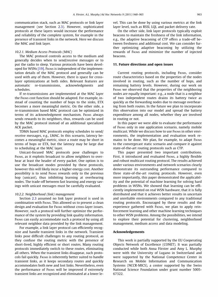
A. Förster, A.L. Murphy / Ad Hoc Networks 9 (2011) 940–965 963
communication stack, such as MAC protocols or link layermanagement (see Section 2.3). However, sophisticatedprotocols at these layers would increase the performanceand reliability of the complete system, for example in thepresence of transient links in the network. Here we discussthe MAC and link layer.
10.2.1. Medium Access Protocols (MAC)The MAC protocol controls access to the medium and
generally decides when to send/receive messages or toput the radio to sleep. Various protocols have been devel-oped for WSNs [19]. FROMS is independent of the implemen-tation details of the MAC protocol and generally can beused with any of them. However, there is space for cross-layer optimizations at both sides. Relevant features areautomatic re-transmissions, acknowledgments andschedules.
If re-transmissions are implemented at the MAC layerthe FROMS cost function should be adapted. For example, in-stead of counting the number of hops to the sinks, ETXbecomes a more meaningful metric. On the other side, are-transmission based MAC protocol can be optimized interms of its acknowledgment mechanism. FROMS alwayssends rewards to its neighbors, thus, rewards can be usedby the MAC protocol instead of an additional specializedACK packet.
TDMA based MAC protocols employ schedules to send/receive messages, e.g., LMAC. In this scenario, latency be-comes a meaningful metric, since a route may be short interms of hops or ETX, but the latency may be large dueto scheduling at the MAC layer.
Unicast-focused MAC protocols pose challenges toFROMS, as it exploits broadcast to allow neighbors to over-hear at least the header of every packet. One option is touse the broadcast modes provided by these protocols,however this will likely incur a higher energy cost. Anotherpossibility is to send FROMS rewards only to the previoushop (unicast), thus inhibiting learning at overhearingnodes. The trade-off between fast learning and energy sav-ings with unicast messages must be carefully evaluated.
10.2.2. Neighborhood (link) managementSection 2.3 assumed no link layer protocol is used in
combination with FROMS. This allowed us to present a cleandesign and evaluation for FROMS without cross-layer issues.However, such a protocol will further optimize the perfor-mance of the system by providing link quality information.FROMS can easily accommodate such a protocol by using allrelevant neighbor data provided by the link management.
For example, a link layer protocol can efficiently recog-nize and handle transient links in the network. Transientlinks pose difficult challenges to any routing protocol, asthey confuse the routing metric with the presence ofshort-lived, highly efficient or short routes. Many routingprotocols immediately switch to these routes, eliminatingall others. When the transient links disappear, such proto-cols fail quickly. FROMS is inherently better suited to handletransient links, as it keeps secondary routes and quicklyaccommodates both new and lost links. Nevertheless, eventhe performance of FROMS will be improved if extremelytransient links are recognized and eliminated at a lower le-
vel. This can be done by using various metrics at the linklayer level, such as RSSI, LQI, and packet delivery rate.
On the other side, link layer protocols typically exploitbeacons to maintain the freshness of the link information,e.g., the adaptive beaconing of CTP offers a trade-off be-tween freshness and additional cost. We can consider fur-ther optimizing adaptive beaconing by utilizing therewards of FROMS and minimize the number of injectedbeacons.
11. Future directions and open issues
Current routing protocols, including FROMS, considerroute characteristics based on the properties of the nodesinvolved in routing, such as the number of hops, andremaining battery levels. However, during our work onFROMS we observed that the properties of the neighboringnodes are equally important: e.g., a node that is a neighborof two independent routes drains its battery twice asquickly as the forwarding nodes due to message overhear-ing from both routes. In the future we plan to incorporatethis observation into our model and spread the batteryexpenditure among all nodes, whether they are involvedin routing or not.
In this paper we were able to evaluate the performanceof FROMS only in one application scenario, namely mobilemulticast. While we discuss how to use FROMS in other envi-ronments, the implementation and evaluation work re-mains to be done. We plan, for example, to adapt FROMS
to the convergecast static scenario and compare it againststate-of-the-art routing protocols such as CTP.
This paper presented two important contributions.First, it introduced and evaluated FROMS, a highly flexibleand robust multicast routing protocol. The results achievedunder various environments and network scenarios clearlydemonstrate its outstanding performance compared tothree state-of-the-art routing protocols. However, evenmore importantly, this paper demonstrated the applicabil-ity and the potential of machine learning for solving hardproblems in WSNs. We showed that learning can be effi-ciently implemented on real WSN hardware, that it is fullydistributed and that it achieves better results in uncertainand unreliable environments compared to any traditionalrouting protocols. Encouraged by these results and theexperience gathered with FROMS, we plan to apply rein-forcement learning and other machine learning techniquesto other WSN problems. Among the possibilities, we intendto explore their potential for clustering, neighborhoodmanagement, medium access and data modeling.
Acknowledgements
This work is partially supported by the EU CooperatingObjects Network of Excellence (CONET). It was partiallyconducted while both Anna Förster and Amy L. Murphywere with the University of Lugano in Switzerland andwere supported by the National Competence Center inResearch on Mobile Information and CommunicationSystems (NCCR-MICS), a center supported by the SwissNational Science Foundation under grant number 5005-67322.
964 A. Förster, A.L. Murphy / Ad Hoc Networks 9 (2011) 940–965
References
[1] J.M. Kahn, R.H. Katz, K.S.J. Pister, Next century challenges: mobilenetworking for ‘‘Smart Dust’’, in: Proceedings of the 5th AnnualACM/IEEE International Conference on Mobile Computing andNetworking (MobiCom), Seattle, WA, USA, 1999, pp. 271–278.
[2] G. Werner-Allen, K. Lorincz, M. Ruiz, O. Marcillo, J. Johnson, J. Lees, M.Welsh, Deploying a wireless sensor network on an active volcano,IEEE Internet Computing 10 (2) (2006) 18–25.
[3] K. Martinez, P. Padhy, A. Riddoch, R. Ong, J. Hart, Glacial environmentmonitoring using sensor networks, in: Proceedings of the 1stWorkshop on Real-World Wireless Sensor Networks (REALWSN),Stockholm, Sweden, 2005, p. 5.
[4] K. Langendoen, A. Baggio, O. Visser, Murphy loves potatoes:experiences from a pilot sensor network deployment in precisionagriculture, in: Proceedings of the 20th International Symposium onParallel and Distributed Processing Symposium (IPDPS), RhodesIsland, Greece, 2006, p. 8.
[5] G. Barrenetxea, F. Ingelrest, G. Schaefer, M. Vetterli, The hitchhiker’sguide to successful wireless sensor network deployments, in:Proceedings of the 6th ACM Conference on Embedded NetworkSensor Systems (SenSys), New York, NY, USA, 2008, pp. 43–56.
[6] E.A. Basha, S. Ravela, D. Rus, Model-based monitoring for earlywarning flood detection, in: Proceedings of the 6th ACM Conferenceon Embedded Network Sensor Systems (SenSys), New York, NY, USA,2008, pp. 295–308.
[7] J. McCulloch, P. McCarthy, S.M. Guru, W. Peng, D. Hugo, A. Terhorst,Wireless sensor network deployment for water use efficiency inirrigation, in: Proceedings of the Workshop on Real-world WirelessSensor Networks (REALWSN), Glasgow, Scotland, 2008, pp. 46–50.
[8] I.F. Akyildiz, W. Su, Y. Sankarasubramaniam, E. Cayirci, Wirelesssensor networks: a survey, Computer Networks 38 (4) (2002) 393–422.
[9] E. Cayirci, T. Coplu, SENDROM: sensor networks for disaster reliefoperations management, Wireless Networks 13 (3) (2007) 409–423.
[10] I.F. Akyildiz, O.A. Akan, C. Chen, J. Fang, W. Su, Interplanetaryinternet: state-of-the-art and research challenges, ComputerNetworks 43 (2) (2003) 75–112.
[11] B. Malakooti, H. Kim, K. Bhasin, Human and robotics technologyspace exploration communication scenarios: characteristics,challenges and scenarios for developing intelligent internetprotocols, in: Proceedings of the 2nd IEEE International Conferenceon Space Mission Challenges for Information Technology (SMC-IT),Pasadena, CA, USA, 2006, pp. 322–329.
[12] B. Raman, K. Chebrolu, Censor networks: a critique of ‘‘sensornetworks’’ from a systems perspective, ACM SIGCOMM ComputerCommunication Review 38 (3) (2008) 75–78.
[13] H. Frey, F. Ingelrest, D. Simplot-Ryl, Localized minimum spanningtree based multicast routing with energy-efficient guaranteeddelivery in ad hoc and sensor networks, in: Proceedings of the 9thIEEE International Symposium on a World of Wireless, Mobile andMultimedia Networks (WOWMOM), Newport Beach, CA, USA, 2008,pp. 1–8.
[14] F. Silva, J. Heidemann, R. Govindan, D. Estrin, Frontiers in DistributedSensor Networks, CRC Press, Inc., 2003. chapter Directed Diffusion, p.25.
[15] A. Förster, A.L. Murphy, FROMS: feedback routing for optimizingmultiple-sinks in WSN with reinforcement learning, in: Proceedings3rd International Conference on Intelligent Sensors, SensorNetworks and Information Processing (ISSNIP), Melbourne,Australia, 2007, pp. 371–376.
[16] A. Förster, A.L. Murphy, Balancing energy expenditure in WSNsthrough reinforcement learning: a study, in: Proceedings of the 1stInternational Workshop on Energy in Wireless Sensor Networks(WEWSN), Santorini Island, Greece, 2008, p. 7.
[17] G. Wittenburg, K. Terfloth, F. López Villafuerte, T. Naumowicz, H.Ritter, J. Schiller, Fence monitoring – experimental evaluation of ause case for wireless sensor networks, in: Proceedings of the 4thEuropean Conference on Wireless Sensor Networks (EWSN), Delft,The Netherlands, 2007, pp. 163–178.
[18] M. Ali, U. Saif, A. Dunkels, T. Voigt, K. Römer, K. Langendoen, J.Polastre, Z. Uzmi, Medium access control issues in sensor networks,SIGCOMM Computation and Communication Review 36 (2) (2006)33–36.
[19] K. Langendoen, Medium access control in wireless sensor networks,in: H. Wu, Y. Pan (Eds.), Medium Access Control in WirelessNetworks, Practice and Standards, vol. II, Nova Science Publishers,Inc., 2007, p. 22.
[20] A. Woo, T. Tong, D. Culler, Taming the underlying challenges ofreliable multihop routing in sensor networks, in: Proceedings of the1st International Conference on Embedded Networked SensorSystems (SenSys), Los Angeles, CA, USA, 2003, pp. 14–27.
[21] G. Werner-Allen, K. Lorincz, J. Johnson, J. Lees, M. Welsh, Fidelityand yield in a volcano monitoring sensor network, in: Proceedingsof the 7th USENIX Symposium on Operating Systems Design andImplementation, USENIX Association, Berkeley, CA, USA, 2006, p.27.
[22] O. Gnawali, R. Fonseca, K. Jamieson, D. Moss, P. Levis, Collection treeprotocol, in: Proceedings of the 7th ACM Conference on EmbeddedNetworked Sensor Systems (SenSys), ACM, Berkeley, California,2009, pp. 1–14.
[23] C.E. Perkins, E.M. Royer, Ad-hoc on-demand distance vector routing,in: Proceedings of the 2nd IEEE Workshop on Mobile ComputerSystems and Applications (WMCSA), New Orleans, USA, 1999, pp.90–100.
[24] R. Vaishampayan, J.J. Garcia-Luna-Aceves, Efficient and robustmulticast routing in mobile ad hoc networks, in: Proceedings ofthe IEEE International Conference on Mobile Ad-hoc and SensorSystems (MASS), Fort Lauderdale, FL, USA, 2004, pp. 304–313.
[25] B.-R. Chen, K.-K. Muniswamy-Reddy, M. Welsh, Ad-hoc multicastrouting on resource-limited sensor nodes, in: Proceedings of the 2ndInternational Workshop on Multi-hop Ad hoc Networks: FromTheory to Reality (REALMAN), Florence, Italy, 2006, pp. 87–94.
[26] B. Karp, H.T. Kung, GPSR: greedy perimeter stateless routing forwireless networks, in: Proceedings of the 6th Annual InternationalConference on Mobile Computing and Networking (MobiCom),Boston, MA, USA, 2000, pp. 243–254.
[27] J.A. Sanchez, P.M. Ruiz, I. Stojmenovic, Energy-efficient geographicmulticast routing for sensor and actuator networks, ComputerCommunications 30 (13) (2007) 2519–2531.
[28] M. Zamalloa, K. Seada, B. Krishnamachari, A. Helmy, Efficientgeographic routing over lossy links in wireless sensor networks,ACM Transactions on Sensor Networks 4 (3) (2008) 1–33.
[29] P. Ciciriello, L. Mottola, G. Picco, Efficient routing from multiplesources to multiple sinks in wireless sensor networks, in:Proceedings of the 4th European Conference on Wireless SensorNetworks (EWSN), Delft, The Netherlands, 2007, pp. 34–50.
[30] Y. Chen, S. Ann, Y. Lin, Ve-mobicast: A variant-egg-based mobicastrouting protocol for sensornets, in: Proceedings of the IEEEInternational Conference on Communications (ICC), Vol. 5, Seoul,Korea, 2005, pp. 3020–3024.
[31] B. Kusy, H. Lee, M. Wicke, N. Milosavljevic, L. Guibas, Predictive qosrouting to mobile sinks in wireless sensor networks, in: Proceedingsof the International Conference on Information Processing in SensorNetworks (IPSN), San Francisco, CA, USA, 2009, pp. 109–120.
[32] H. Luo, F. Ye, J. Cheng, S. Lu, L. Zhang, TTDD: two-tier datadissemination in large-scale wireless sensor networks, WirelessNetworks 11 (1–2) (2005) 161–175.
[33] H. Kim, T. Abdelzaher, W. Kwon, Minimum-energy asynchronousdissemination to mobile sinks in wireless sensor networks, in:Proceedings of the 1st International Conference on EmbeddedNetworked Sensor Systems (SenSys), Los Angeles, CA, USA, 2003,pp. 193–204.
[34] H. Kim, T. Abdelzaher, W. Kwon, Dynamic delay-constrainedminimum-energy dissemination in wireless sensor networks,Transactions on Embedded Computing Systems 4 (3) (2005) 679–706.
[35] R. Flury, R. Wattenhofer, Routing, anycast, and multicast for meshand sensor networks, in: Proceedings of the 26th IEEE InternationalConference on Computer Communications (INFOCOM), 2007, pp.946–954.
[36] S. Kulkarni, A. Förster, G. Venayagamoorthy, A survey on applicationsof computational intelligence for wireless sensor networks, IEEECommunications Surveys & Tutorials 13 (1) (2011) 25.
[37] R. Arroyo-Valles, R. Alaiz-Rodrigues, A. Guerrero-Curieses, J. Cid-Suiero, Q-probabilistic routing in wireless sensor networks, in:Proceedings of the 3rd International Conference on IntelligentSensors, Sensor Networks and Information Processing (ISSNIP),Melbourne, Australia, 2007, pp. 1–6.
[38] J.A. Boyan, M.L. Littman, Packet routing in dynamically changingnetworks: a reinforcement learning approach, Advances in NeuralInformation Processing Systems 6 (1994) 671–678.
[39] P. Beyens, M. Peeters, K. Steenhaut, A. Nowe, Routing withcompression in wireless sensor networks: a Q-learning approach,in: Proceedings of the 5th European Workshop on Adaptive Agentsand Multi-Agent Systems (AAMAS), Paris, France, 2005, p. 12.
A. Förster, A.L. Murphy / Ad Hoc Networks 9 (2011) 940–965 965
[40] R.S. Sutton, A.G. Barto, Reinforcement Learning: An Introduction, TheMIT Press, 1998.
[41] C. Watkins, Learning from delayed rewards, Ph.D. thesis, CambridgeUniversity, Cambridge, England, 1989.
[42] U. Brandes, T. Erlebach, Network Analysis – MethodologicalFoundations, Springer-Verlag, Berlin, Germany, 2005.
[43] L. Sang, A. Arora, H. Zhang, On link asymmetry and one-wayestimation in wireless sensor networks, ACM Transactions on SensorNetworks 6 (2) (2010) 1–25.
[44] A. Egorova-Förster, A.L. Murphy, A feedback enhanced learningapproach for routing in WSN, in: Proceedings of the 4th Workshopon Mobile Ad-Hoc Networks (WMAN), Springer-Verlag, Berlin,Switzerland, 2007, pp. 12.
[45] A. Förster, A.L. Murphy, J. Schiller, K. Terfloth, An efficientimplementation of reinforcement learning-based routing on realWSN hardware, in: Proceedings of the 4th IEEE InternationalConference on Wireless and Mobile Computing, Networking andCommunications (WiMOB), Avignon, France, 2008, p. 8.
[46] A. Förster, A.L. Murphy, FROMS: A failure tolerant and mobilityenabled multicast routing paradigm with reinforcement learning forWSNs, Tech. Rep. TR 2009/04, University of Lugano, June 2009.
[47] D. Puccinelli, M. Haenggi, Reliable data delivery in large-scale low-power sensor networks, ACM Transactions on Sensor Networks 6 (4)(2010) 41.
[48] A. Kuntz, F. Schmidt-Eisenlohr, O. Graute, H. Hartenstein, M.Zitterbart, Introducing probabilistic radio propagation models inOMNeT++ mobility framework and cross validation check with NS-2,in: Proceedings of the 1st International Workshop on OMNeT++,Marseille, France, 2008, p. 7.
[49] J. Polastre, J. Hill, D. Culler, Versatile low power media access forwireless sensor networks, in: Proceedings of the 2nd ACMConference on Embedded Networked Sensor Systems (SenSys),Baltimore, MD, USA, 2004, pp. 95–107.
[50] L. van Hoesel, P. Havinga, A lightweight medium access protocol(LMAC) for wireless sensor networks, in: Proceedings of the 1stInternational Conference on Networked Sensing Systems (INSS),Tokyo, Japan, 2004, pp. 946–953.
[51] Scatterweb Inc. <http://www.scatterweb.de/>.[52] G. Werner-Allen, P. Swieskowski, M. Welsh, Motelab: a wireless
sensor network testbed, in: Proceedings of the 4th InternationalSymposium on Information Processing in Sensor Networks (IPSN),2005, pp. 483–488.
[53] K. Zawadzki, A. Förster, Simulating routing protocols for wirelesssensor networks, bachelor thesis at the University of Lugano, 2008.
Anna Förster is currently a postdoctoralresearcher at the Networking Laboratory ofthe University of Applied Sciences of SouthernSwitzerland. She received a M.S. Degree inComputer Science and Aerospace Engineeringfrom the Free University in Berlin, Germany,in 2005 and a PhD Degree in Computer Sci-ence from the University of Lugano, Switzer-land, in 2009. Her main research topicsinclude machine learning applications towireless ad hoc communications, program-ming and deployment of wireless sensor net-
works, and communication issues in the interplanetary internet. Hermain goal is to exploit the full potential of intelligent, self-organized adhoc networks and to make wireless sensor networks user-friendly and
easily accessible to everybody. http://www.dti.supsi.ch/�afoerste.Amy L. Murphy is currently a researcher atFBK-irst. She received a B.S. in Computer Sci-ence from the University of Tulsa in 1995, andM.S. and D.Sc. degrees from WashingtonUniversity in St. Louis, Missouri in 1997 and2000 respectively. She spent 5 years in aca-demia as an assistant professor at the Uni-versity of Rochester, New York, and theUniversity of Lugano, Switzerland, and 1 yearas a visiting researcher at Politecnico diMilano, Italy. Her research interests includethe design, specification, and implementation
of middleware systems for sensor, mobile ad hoc, and dynamic peer topeer networks. The driving theme of the work is to enable the rapiddevelopment of dependable applications for these complex dynamic
environments. http://es.fbk.eu/people/murphy/.