Embed Size (px)
Citation preview
Functional Mock-up Interface
for Model Exchange
MODELICA Association Project FMI
Document version: 1.0.1
July 2017
• ••• ••• ••• •• ••• ••• •• ••• ••• ••• •• • •• ••• •• ••• ••• ••• •• ••• ••• •• ••• ••
Functional Mock-up Interface for Model Exchange
FMI Project, MODELICA Association
July, 2017
Page 2 of 56
History
Version Date Remarks
1.0 2010-01-26 First version
1.0.1 2016-05-05 AJunghanns: worked changes from ticket #370 into document, first attempt
Second run AJunghanns and AViel
1.0.1 2017-07-10 FMI Steering Committee releases
License of this document
Copyright © 2017, MODELICA Association Project FMIThis document is provided “as is" without any
warranty. It is licensed under the CC-BY-SA (Creative Commons Attribution-Sharealike 3.0 Unported)
license, i.e., the license used by Wikipedia. Human-readable summary of the license text from
http://creativecommons.org/licenses/by-sa/3.0/:
You are free:
to Share — to copy, distribute and transmit the work, and
to Remix — to adapt the work
Under the following conditions:
Attribution — You must attribute the work in the manner specified by the author or
licensor (but not in any way that suggests that they endorse you or your use of the work.)
Share Alike — If you alter, transform, or build upon this work, you may distribute the resulting
work only under the same, similar or a compatible license.
The legal license text and disclaimer is available at:
http://creativecommons.org/licenses/by-sa/3.0/legalcode
Note:
Article (3a) of this license requires that modifications of this work must clearly label, demarcate or
otherwise identify that changes were made.
The C-header and XML-schema files that accompany this document are available under the BSD
license (http://www.opensource.org/licenses/bsd-license.html) with the extension that modifications
must be also provided under the BSD license.
If you have improvement suggestions, please send them to the FMI development group at
All contributors have signed the FMI Corporate Contributor License Agreement (CCLA).
Functional Mock-up Interface for Model Exchange
FMI Project, MODELICA Association
July, 2017
Page 3 of 56
Abstract
This document defines the “Functional Mock-up Interface for Model Exchange”. The intention is that a
modelling environment can generate C-Code of a dynamic system model that can be utilized by other
modelling and simulation environments. Models are described by differential, algebraic and discrete
equations with time-, state- and step-events. The models to be treated by this interface can be large for
usage in offline or online simulation or can be used in embedded control systems on micro-processors. It
is possible to utilize several instances of a model and to connect models hierarchically together. A model
is independent of the target simulator because it does not use a simulator specific header file as in other
approaches.
A model is distributed in one zip-file that contains several files:
(1) An xml-file contains the definition of all variables in the model and other model information. It is then
possible to run the model on a target system without this information, i.e., with no unnecessary overhead.
(2) All needed model equations are provided with a small set of easy to use C-functions. A new caching
technique allows a more efficient evaluation of the model equations as in other approaches. These C-
functions can either be provided in source and/or binary form. Binary forms for different platforms can be
included in the same model zip-file.
(3) Further data can be included in the zip-file, especially a model icon (bitmap file), documentation files,
maps and tables needed by the model, and/or all object libraries or DLLs that are utilized.
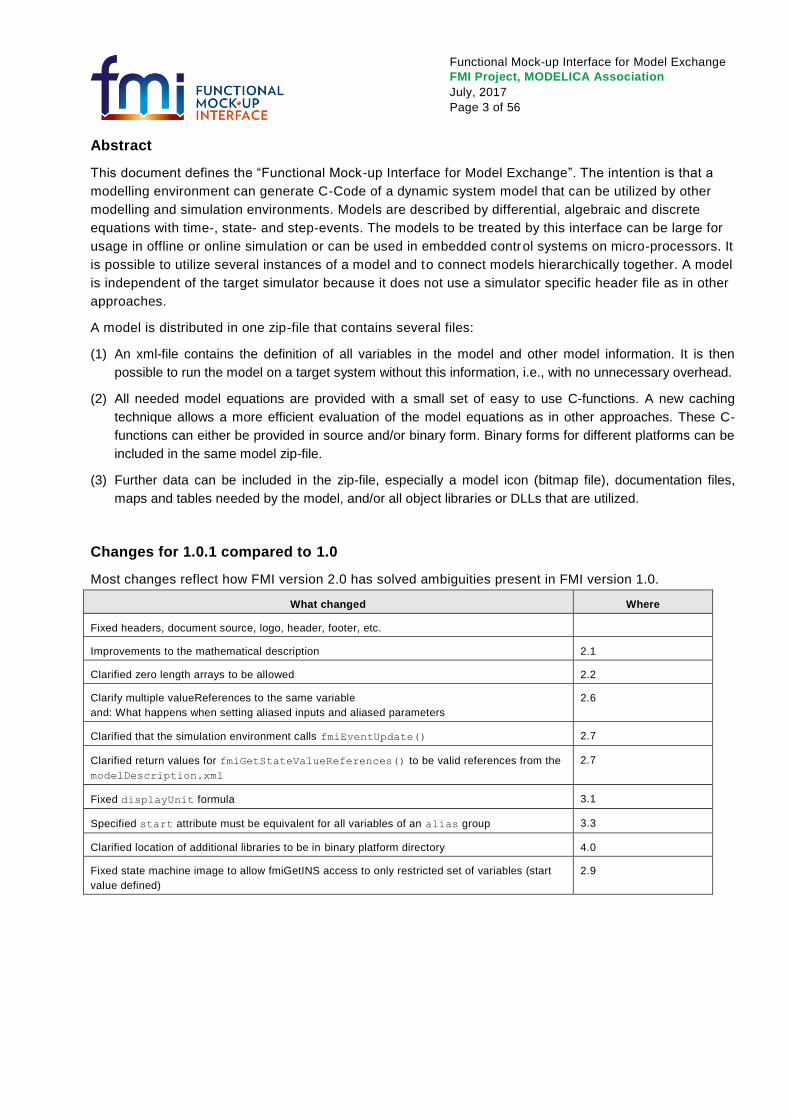
Changes for 1.0.1 compared to 1.0
Most changes reflect how FMI version 2.0 has solved ambiguities present in FMI version 1.0.
What changed Where
Fixed headers, document source, logo, header, footer, etc.
Improvements to the mathematical description 2.1
Clarified zero length arrays to be allowed 2.2
Clarify multiple valueReferences to the same variable
and: What happens when setting aliased inputs and aliased parameters
2.6
Clarified that the simulation environment calls fmiEventUpdate() 2.7
Clarified return values for fmiGetStateValueReferences() to be valid references from the
modelDescription.xml
2.7
Fixed displayUnit formula 3.1
Specified start attribute must be equivalent for all variables of an alias group 3.3
Clarified location of additional libraries to be in binary platform directory 4.0
Fixed state machine image to allow fmiGetINS access to only restricted set of variables (start
value defined)
2.9
Functional Mock-up Interface for Model Exchange
FMI Project, MODELICA Association
July, 2017
Page 4 of 56
Contents
1. Overview ........................................................................................................................................ 5
1.1. Properties and Guiding Ideas ................................................................................................. 6
1.2. Acknowledgements ................................................................................................................ 8
2. Model Interface ............................................................................................................................. 9
2.1. Mathematical Description ....................................................................................................... 9
2.2. Platform Dependent Definitions (fmiModelTypes.h) .............................................................. 12
2.3. Status Returned by Functions .............................................................................................. 14
2.4. Inquire Platform and Version Number of Header Files .......................................................... 14
2.5. Creation and Destruction of Model Instances ....................................................................... 15
2.6. Providing Independent Variables and Re-initialization of Caching ......................................... 16
2.7. Evaluation of Model Equations ............................................................................................. 18
2.8. External Models ................................................................................................................... 21
2.9. State Machine of Calling Sequence ...................................................................................... 22
2.10. Example ............................................................................................................................... 23
3. Model Description Schema ......................................................................................................... 26
3.1. Description of a Model (fmiModelDescription) ....................................................................... 27
3.2. Definition of a Type (fmiType) .............................................................................................. 31
3.3. Definition of a Scalar Variable (fmiScalarVariable) ............................................................... 33
3.4. Example ............................................................................................................................... 38
4. Model Distribution ...................................................................................................................... 40
5. Literature ..................................................................................................................................... 42
Appendix A Contributors ................................................................................................................ 43
A.1 Version 1.0 .......................................................................................................................... 43
Appendix B Implementation Issues................................................................................................ 44
B.1 Variable Naming Conventions .............................................................................................. 44
B.2 Event Detection.................................................................................................................... 45
B.3 Dynamic State Selection ...................................................................................................... 47
B.4 Variable Caching .................................................................................................................. 47
B.5 Connecting FMUs together ................................................................................................... 48
Appendix C Features for Future Versions ..................................................................................... 52
Appendix D Glossary ...................................................................................................................... 55
Functional Mock-up Interface for Model Exchange
FMI Project, MODELICA Association
July, 2017
Page 5 of 56
1. Overview
The FMI (Functional Mock-up Interface) defines an interface to be implemented by an executable called
FMU (Functional Mock-up Unit). The FMI functions are used (called) by a simulator to create one or
more instances of the FMU, called models, and to run these models, typically together with other
models. An FMU may either be self-integrating (co-simulation) or require the simulator to perform
numerical integration. In this document, the interface for the latter case is defined1.
The goal is to describe models of dynamic systems, i.e., models defined by differential, algebraic and
discrete equations and to provide an interface to evaluate these equations as needed in different simulation
environments, as well as in embedded control systems, with explicit or implicit integrators and fixed or
variable step-size. The interface is designed so that large models can be described and consists of the
following parts:
Model Interface
All needed equations are evaluated by calling standardized “C” functions. “C” is used, because it is
the most portable programming language today and is the only programming language that can be
utilized in all embedded control systems.
Model Description Schema
The schema defines the structure and content of an xml-file generated by a modelling environment.
This xml-file contains the definition of all variables in the model in a standardized way. It is then
possible to run the C-code in an embedded system without the overhead of the variable definition
(the alternative would be to store this information in the C-code and access it via function calls, but
this is not practical for embedded systems and not for large models). Furthermore, the variable
definition is a complex data structure and tools should be free how to represent this data structure in
their programs. The selected approach allows a tool to store and access the variable definitions
(without any memory or efficiency overhead of standardized access functions) in the programming
language of the simulation environment, usually C++, C# or Java. Note, there are many free and
commercial libraries in different programming languages to read xml-files in to an appropriate data
structure, see, e.g., http://en.wikipedia.org/wiki/Xml#Parsers.
A model is distributed in one zip-file. The zip-file contains (more details are given in section 4):
The Model Description File (xml format).
The C sources of the Model Interface (including the needed run-time libraries used in the model)
and/or
Dynamic link libraries (DLL) for one or several target machines. This solution is especially used,
if the model provider wants to hide the model source code to secure the contained know-how. A
model may contain physical parameters or geometrical dimensions, which should not be open.
On the other hand, some functionality requires source code.
Additional model data (like tables, maps) in model specific file formats.
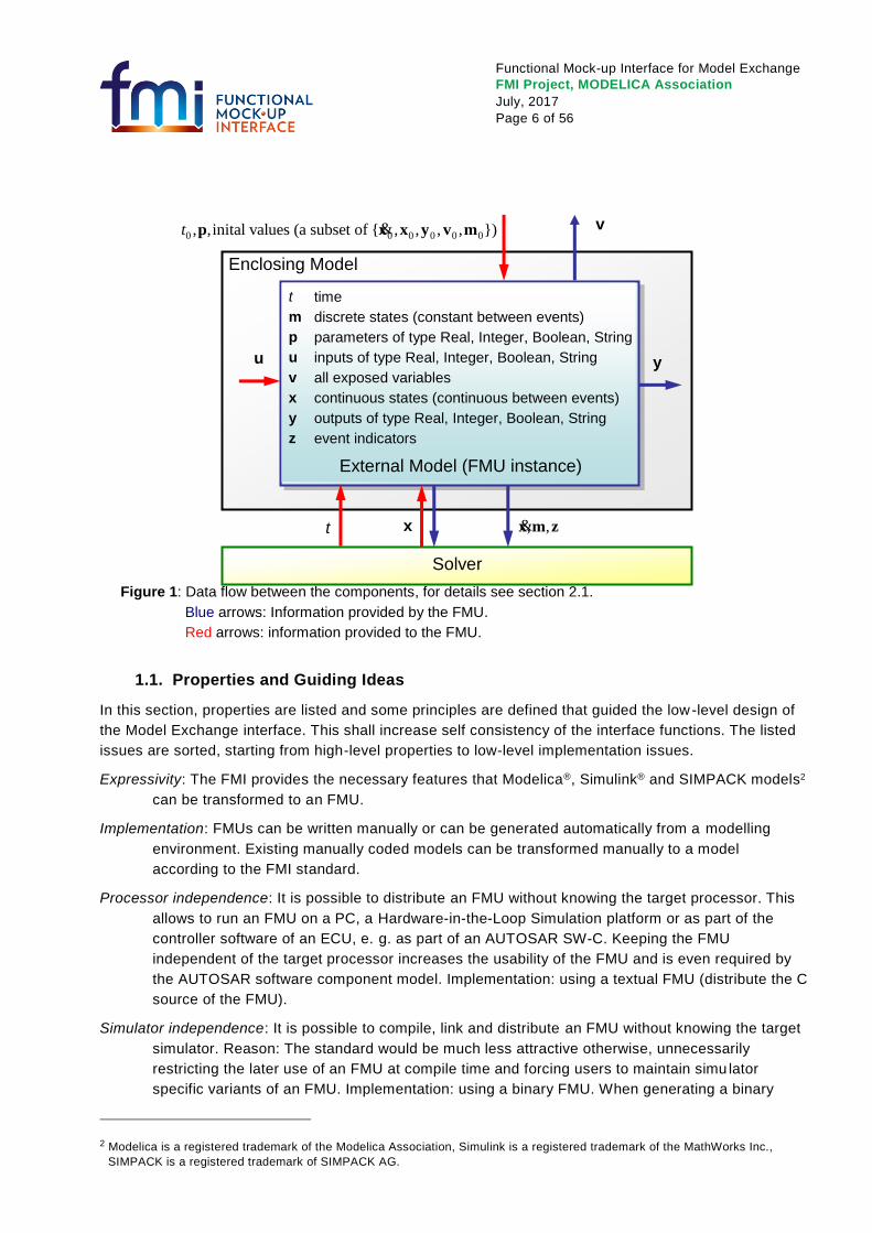
A schematic view of a model in “FMI for Model Exchange” format is shown in the next figure:
1 A simple form of co-simulation is also possible with this interface, by treating a co-simulated model as a discrete system.
Functional Mock-up Interface for Model Exchange
FMI Project, MODELICA Association
July, 2017
Page 6 of 56
Figure 1: Data flow between the components, for details see section 2.1.
Blue arrows: Information provided by the FMU.
Red arrows: information provided to the FMU.
1.1. Properties and Guiding Ideas
In this section, properties are listed and some principles are defined that guided the low-level design of
the Model Exchange interface. This shall increase self consistency of the interface functions. The listed
issues are sorted, starting from high-level properties to low-level implementation issues.
Expressivity: The FMI provides the necessary features that Modelica®, Simulink® and SIMPACK models2
can be transformed to an FMU.
Implementation: FMUs can be written manually or can be generated automatically from a modelling
environment. Existing manually coded models can be transformed manually to a model
according to the FMI standard.
Processor independence: It is possible to distribute an FMU without knowing the target processor. This
allows to run an FMU on a PC, a Hardware-in-the-Loop Simulation platform or as part of the
controller software of an ECU, e. g. as part of an AUTOSAR SW-C. Keeping the FMU
independent of the target processor increases the usability of the FMU and is even required by
the AUTOSAR software component model. Implementation: using a textual FMU (distribute the C
source of the FMU).
Simulator independence: It is possible to compile, link and distribute an FMU without knowing the target
simulator. Reason: The standard would be much less attractive otherwise, unnecessarily
restricting the later use of an FMU at compile time and forcing users to maintain simu lator
specific variants of an FMU. Implementation: using a binary FMU. When generating a binary
2 Modelica is a registered trademark of the Modelica Association, Simulink is a registered trademark of the MathWorks Inc.,
SIMPACK is a registered trademark of SIMPACK AG.
Solver
u y
Enclosing Model
x t , ,x m z&
v 0 0 0 0 0 0, ,inital values (a subset of { , , , , })t p x x y v m&
t time
m discrete states (constant between events)
p parameters of type Real, Integer, Boolean, String
u inputs of type Real, Integer, Boolean, String
v all exposed variables
x continuous states (continuous between events)
y outputs of type Real, Integer, Boolean, String
z event indicators
External Model (FMU instance)
Functional Mock-up Interface for Model Exchange
FMI Project, MODELICA Association
July, 2017
Page 7 of 56
FMU, e. g. a Windows dynamic link library (.dll) or a Linux shared object library (.so), the target
operating system and eventually the target processor must be known. However, no run-time
libraries, source files or header files of the target simulator are needed to generate the binary
FMU. As a result, the binary FMU can be executed by any simulator running on the target
platform (provided the necessary licenses are available, if required from the model or from the
used run-time libraries).
Small run-time overhead : Communication between an FMU and a target simulator through the FMI does
not introduce significant run time overhead. This is achieved by a new cach ing technique (to
avoid to compute the same variables several time) and by exchanging vectors instead of scalar
quantities.
Small footprint: A compiled FMU (the executable) is small. Reason: An FMU may run on an ECU
(Electronic Control Unit, e.g., a micro processor), and ECUs have strong memory limitations.
This is achieved by storing signal attributes (names, units, etc.) and all other information not
needed for model evaluation in a separate text file (= Model Description File) that is not needed
on the micro processor where the executable might run.
Hide data structure: The FMI for Model Exchange does not prescribe a data structure (a C struct) to
represent a model. Reason: the FMI standard shall not unnecessarily restrict or prescribe a
certain implementation of FMUs or simulators (whoever holds the model data), to ease
implementation by different tool vendors.
Support many and nested FMUs: A simulator can run many FMUs in a single simulation run. The inputs
and outputs of these FMUs can be connected with direct feed through. Moreover, an FMU may
contain nested FMUs.
Numerical Robustness: The FMI standard allows that problems which are numerically critical (e.g. time
and state events, multiple sample rates, stiff problems) can be treated in a robust way.
Hide cache: A typical FMU will cache computed results for later reuse. To simplify usage and to reduce
error possibilities by a simulator, the caching mechanism is hidden from the FMI. Reason: First,
the FMI should not force an FMU to implement a certain caching policy. Second, this helps to
keep the FMI simple. Implementation: The FMI provides explicit methods (called by the
simulator) for setting properties that invalidate cached data. An FMU that chooses to implement
a cache may maintain a set of 'dirty' flags, hidden from the simulator. A get method, e. g. to a
state, will then either trigger a computation, or return cached data, depending on the value of
these flags.
Support numerical solvers: A typical target simulator will use numerical solvers. These solvers require
vectors for states, derivatives and zero-crossing functions. The FMU directly fills the values of
such vectors provided by the solvers. Reason: minimize execution time. The exposure of these
vectors conflicts somewhat with the 'hide data structure' requirement, but the efficiency gain
justifies this.
Explicit signature: The intended operations, argument types and return values are made explicit in the
signature. For example, an operator (such as 'compute_derivatives') is not passed as an int
argument but a special function is called for this. The 'const' prefix is used for any pointer that
should not be changed, including 'const char*' instead of 'char*'. Reason: the correct use of the
FMI can be checked at compile time and allow calling of the C code in a C++ environment (which
is much stricter on ‘const’ as C is). This will help to develop FMUs that use the FMI in the
intended way.
Functional Mock-up Interface for Model Exchange
FMI Project, MODELICA Association
July, 2017
Page 8 of 56
Few functions: The FMI consists of a few, 'orthogonal' functions, avoiding redundant functions, that could
be defined in terms of others. Reason: This leads to a compact, easy to use, and hence
attractive API with a compact documentation (the essential part is less than 30 pages).
Error handling: All FMI methods use a common set of methods to communicate errors.
Allocator must free: All memory (and other resources) allocated by the FMU are freed (released) by the
FMU. Likewise, resources allocated by the simulator are released by the simulator. Reason: this
helps to prevent memory leaks.
Immutable strings: All strings passed as arguments or returned are read-only and must not be modified
by the receiver. Reason: This eases the reuse of strings.
Use C: The FMI is encoded using C, not C++. Inheritance of sub-interfaces can be implemented using
#include. Reason: Avoid problems with compiler and linker dependent behavior. Run FMU on
embedded target.
This version of the functional mock-up interface does not have the following desirable properties. They
might be added in a future version:
The interface is for ordinary differential equations in state space form (ODE). It is not for a general
differential-algebraic equation system.
Special features as might be useful for multi-body system programs, like SIMPACK, are not included.
The interface is for simulation and for embedded systems. Properties that might be additionally
needed for optimization are not included.
No Jacobian matrix (neither dense nor sparse; tools have to derive this matrix numerically). The goal
for the future is that large models, i. e., models with up to 104 continuous states and up to 106
variables, can be handled.
No linearization data (A,B,C,D matrices of linearized model)
No explicit definition of the variable hierarchy in the xml file.
The number of states and number of event indicators are fixed and cannot be changed.
Parameters are constant although it would be useful to change them online, e.g., for real-time training
simulators.
1.2. Acknowledgements
This work was carried out within the ITEA2 MODELISAR project (project number: ITEA 2 – 07006,
www.itea2.org/public/project_leaflets/MODELISAR_profile_oct-08.pdf).
Daimler AG, DLR, ITI GmbH, QTronic GmbH and SIMPACK AG thank BMBF for partial funding of this
work within MODELISAR (BMBF Förderkennzeichen: 01lS08002).
Dynasim AB thanks the Swedish funding agency VINNOVA (2008-02291) for partial funding of this work
within MODELISAR.
LMS Imagine thanks DGCIS for partial funding of this work within MODELISAR.
Functional Mock-up Interface for Model Exchange
FMI Project, MODELICA Association
July, 2017
Page 9 of 56
2. Model Interface
This chapter contains the interface description to access the equations of a dynamic system from a C
program. Two header files are provided that define the interface. In both header files the convention is
used that all C-functions and type definitions start with the prefix “ fmi”:
“fmiModelTypes.h”
contains the type definitions for the input and output arguments of the functions. This header file must
be used both by the model and by the target simulator. If the target simulator has different definitions
in the header file (e.g., “typedef float fmiReal” instead of “typedef double fmiReal”), then
the model needs to be re-compiled with the header file used by the target simulator. Note, the header
file platform for which the model was compiled can be inquired in the target simulator with function
fmiGetModelTypesPlatform(), see section 2.4.
“fmiModelFunctions.h”
contains the function prototypes that can be accessed in simulation environments and that are defined
in this chapter. This header file, includes “fmiModelTypes.h”. Note, the header file version number
for which the model was compiled, can be inquired in the target simulator with function
fmiGetVersion(), see section 2.4.
The goal is that both textual and binary representations of models are supported and that several models
might be present at the same time in an executable (e.g., model A may use a model B). In order that t his
is possible, the names of the functions in different models must be different or function pointers must be
used. For simplicity, the first variant is utilized here by providing macros in “fmiModelFunctions.h” to
build the actual function names. A typical implementation of the Model Exchange functions is as follows:
#define MODEL_IDENTIFIER MyModel
#include "fmiModelFunctions.h"
< implementation of the Model Exchange functions >
A function that is defined as “fmiGetDerivatives” is changed by the macros to the actual function
name “MyModel_fmiGetDerivatives”, i.e., the function name is prefixed with the model name and an
“_”. The “MODEL_IDENTIFIER” is defined in the Model Description File as attribute
“modelIndentifier”, see section 3.1. A simulation environment can therefore construct the relevant
function names by (a) generating code for the actual function call or (b) by dynamically loading a
dynamic link library and explicitly importing the function symbols by providing the “real” function names
as strings.
In the following sections, the types and the functions of the Model Exchange C-Interface as defined in
the two header files are discussed in detail.
2.1. Mathematical Description
The goal of the Model Exchange interface is to numerically solve a system of differential, algebraic and
discrete equations. In this version of the interface, ordinary differential equations in state space form with
events are handled (abbreviated as “hybrid ODE”).
This type of system is described as a piecewise continuous system. Discontinuities can occur at time
instants t0, t1, … tn, where ti < ti+1. These time instants are called “events”. Events can be known before hand
(= time event), or are defined implicitly (= state and step events).
The “state” of a hybrid ODE is represented by a continuous state x(t) and by a time-discrete state m(t)
that have the following properties:
Functional Mock-up Interface for Model Exchange
FMI Project, MODELICA Association
July, 2017
Page 10 of 56
x(t) is a vector of real numbers (= time-continuous states) and is a continuous function of time inside
each interval ti ≤ t < ti+1 .
m(t) is a set of real, integer, logical, and string variables (= time-discrete states) that is constant inside each
interval ti ≤ t < ti+1. In other words, m(t) changes value only at events. This means, m(t) = m(ti), for ti ≤ t < ti+1.
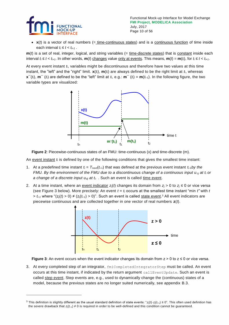
At every event instant ti, variables might be discontinuous and therefore have two values at this time
instant, the ”left” and the ”right” limit. x(ti), m(ti) are always defined to be the right limit at ti, whereas
x¯(ti), m¯ (ti) are defined to be the “left” limit at ti, e.g.: m¯ (ti) = m(ti-1). In the following figure, the two
variable types are visualized:
Figure 2: Piecewise-continuous states of an FMU: time-continuous (x) and time-discrete (m).
An event instant ti is defined by one of the following conditions that gives the smallest time instant:
1. At a predefined time instant ti = Tnext(ti-1) that was defined at the previous event instant ti-1by the
FMU. By the environment of the FMU due to a discontinuous change of a continuous input u cj at ti or
a change of a discrete input udj at ti. . Such an event is called time event.
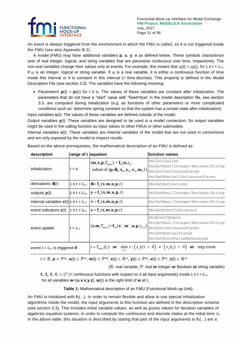
2. At a time instant, where an event indicator zj(t) changes its domain from zj > 0 to zj ≤ 0 or vice versa
(see Figure 3 below). More precisely: An event t = ti occurs at the smallest time instant “min t” with t
> ti-1 where “(zj(t) > 0) ≠ (zj(ti-1) > 0)”. Such an event is called state event.3 All event indicators are
piecewise continuous and are collected together in one vector of real numbers z(t).
Figure 3: An event occurs when the event indicator changes its domain from z > 0 to z ≤ 0 or vice versa.
3. At every completed step of an integrator, fmiCompletedIntegratorStep must be called. An event
occurs at this time instant, if indicated by the return argument callEventUpdate. Such an event is
called step event. Step events are, e.g., used to dynamically change the (continuous) states of a
model, because the previous states are no longer suited numerically, see appendix B.3.
3 This definition is slightly different as the usual standard definition of state events: “zj(t)·zj(ti-1) ≤ 0”. This often used definition has
the severe drawback that zj(ti-1) ≠ 0 is required in order to be well-defined and this condition cannot be guaranteed.
time t
t0 t1 t2
x(t)
m(t)
m–(t1) m(t1)
time
t0 t1 t2
z(t) z > 0
z ≤ 0
Functional Mock-up Interface for Model Exchange
FMI Project, MODELICA Association
July, 2017
Page 11 of 56
An event is always triggered from the environment in which the FMU is called, so it is not triggered inside
the FMU (see also Appendix B.2).
A model (FMU) may have additional variables p, u, y, v as defined below. These symbols characterize
sets of real integer, logical, and string variables that are piecewise continuous over time, respectively. The
non-real variables change their values only at events. For example, this means that uj(t) = uj(ti), for ti ≤ t < ti+1,
if uj is an integer, logical or string variable. If uj is a real variable, it is either a continuous function of time
inside this interval or it is constant in this interval (= time-discrete). This property is defined in the Model
Description File (see section 3.3). The variables have the following meaning:
Parameters p(t) = p(t0) for t ≥ t0. The values of these variables are constant after initialization. The
parameters that do not have a “start” value with “fixed=true” in the model description file, see section
3.3, are computed during initialization (e.g. as functions of other parameters or more complicated
conditions such as: determine spring constant so that the system has a certain state after initialization).
Input variables u(t). The values of these variables are defined outside of the model.
Output variables y(t). These variables are designed to be used in a model connection. So output variables
might be used in the calling function as input values to other FMUs or other submodels.
Internal variables v(t). These variables are internal variables of the model that are not used in connections
and are only exposed by the model to inspect results.
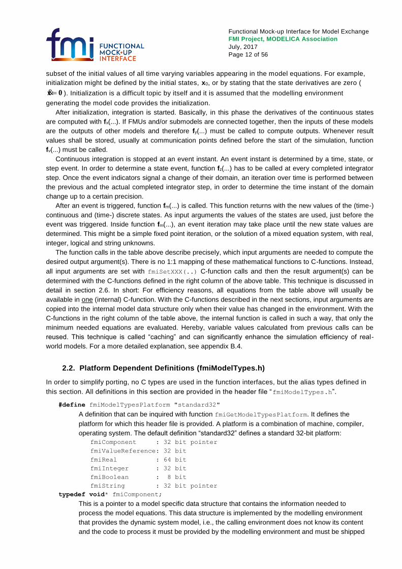
Based on the above prerequisites, the mathematical description of an FMU is defined as:
description range of t equation function names
initialization t = t0
0 0
0 0 0 0 0
( , , , ) = ( , ,
subset of { , , , , , })
nextT tm x p f u
p x x y v m&
fmiInitialize
fmiGetReal/Integer/Boolean/String
fmiGetContinuousStates
fmiGetNominalContinuousStates
derivatives ( )tx& ti ≤ t < ti+1 ( , , , , )x tx f x m u p& fmiGetDerivatives
outputs y(t) ti ≤ t < ti+1 ( , , , , )y ty f x m u p fmiGetReal/Integer/Boolean/String
internal variables v(t) ti ≤ t < ti+1 ( , , , , )v tv f x m u p fmiGetReal/Integer/Boolean/String
event indicators z(t) ti ≤ t < ti+1 ( , , , , )z tz f x m u p fmiGetEventIndicators
event update t = ti+1 1( , , )= ( , , , , )next m iT t x m f x m u p
fmiEventUpdate
fmiGetReal/Integer/Boolean/String
fmiGetContinuousStates
fmiGetNominalStates
fmiGetStateValueReferences
event t = ti+1 is triggered if ( ) min : ( ) 0 ( ) 0 step eventi
next i j j it t
t T t t z t z t
or or
t ∈ ℝ, p ∈ ℙnp, u(t) ∈ ℙnu, m(t) ∈ ℙnm, x(t) ∈ ℝnx, y(t) ∈ ℙny, v(t) ∈ ℙnv, z(t) ∈ ℝnz
(ℝ: real variable; ℙ: real or integer or Boolean or string variable)
fx, fy, fv, fz ∈ C0 (= continuous functions with respect to 4 all input arguments) inside ti ≤ t < ti+1
for all variables w={u,v,x,y,z}: w(ti) is the right limit of w at ti.
Table 1: Mathematical description of an FMU (Functional Mock-up Unit).
An FMU is initialized with f0(...). In order to remain flexible and allow to use special initialization
algorithms inside the model, the input arguments to this function are defined in the description schema
(see section 3.3). This includes initial variable values, as well as guess values for iteration variables of
algebraic equation systems, in order to compute the continuous and discrete states at the initial time t0.
In the above table, this situation is described by stating that part of the input arguments to f0(...) are a
Functional Mock-up Interface for Model Exchange
FMI Project, MODELICA Association
July, 2017
Page 12 of 56
subset of the initial values of all time varying variables appearing in the model equations. For example,
initialization might be defined by the initial states, x0, or by stating that the state derivatives are zero (
x 0& ). Initialization is a difficult topic by itself and it is assumed that the modelling environment
generating the model code provides the initialization.
After initialization, integration is started. Basically, in this phase the derivatives of the continuous states
are computed with fx(...). If FMUs and/or submodels are connected together, then the inputs of these models
are the outputs of other models and therefore fy(...) must be called to compute outputs. Whenever result
values shall be stored, usually at communication points defined before the start of the simulation, function
fv(...) must be called.
Continuous integration is stopped at an event instant. An event instant is determined by a time, state, or
step event. In order to determine a state event, function fz(...) has to be called at every completed integrator
step. Once the event indicators signal a change of their domain, an iteration over time is performed between
the previous and the actual completed integrator step, in order to determine the time instant of the domain
change up to a certain precision.
After an event is triggered, function fm(...) is called. This function returns with the new values of the (time-)
continuous and (time-) discrete states. As input arguments the values of the states are used, just before the
event was triggered. Inside function fm(...), an event iteration may take place until the new state values are
determined. This might be a simple fixed point iteration, or the solution of a mixed equation system, with real,
integer, logical and string unknowns.
The function calls in the table above describe precisely, which input arguments are needed to compute the
desired output argument(s). There is no 1:1 mapping of these mathematical functions to C-functions. Instead,
all input arguments are set with fmiSetXXX(..) C-function calls and then the result argument(s) can be
determined with the C-functions defined in the right column of the above table. This technique is discussed in
detail in section 2.6. In short: For efficiency reasons, all equations from the table above will usually be
available in one (internal) C-function. With the C-functions described in the next sections, input arguments are
copied into the internal model data structure only when their value has changed in the environment. With the
C-functions in the right column of the table above, the internal function is called in such a way, that only the
minimum needed equations are evaluated. Hereby, variable values calculated from previous calls can be
reused. This technique is called “caching” and can significantly enhance the simulation efficiency of real-
world models. For a more detailed explanation, see appendix B.4.
2.2. Platform Dependent Definitions (fmiModelTypes.h)
In order to simplify porting, no C types are used in the function interfaces, but the alias types defined in
this section. All definitions in this section are provided in the header file “fmiModelTypes.h”.
#define fmiModelTypesPlatform "standard32"
A definition that can be inquired with function fmiGetModelTypesPlatform. It defines the
platform for which this header file is provided. A platform is a combination of machine, compiler,
operating system. The default definition “standard32” defines a standard 32-bit platform:
fmiComponent : 32 bit pointer
fmiValueReference: 32 bit
fmiReal : 64 bit
fmiInteger : 32 bit
fmiBoolean : 8 bit
fmiString : 32 bit pointer
typedef void* fmiComponent;
This is a pointer to a model specific data structure that contains the information needed to
process the model equations. This data structure is implemented by the modelling environment
that provides the dynamic system model, i.e., the calling environment does not know its content
and the code to process it must be provided by the modelling environment and must be shipped
Functional Mock-up Interface for Model Exchange
FMI Project, MODELICA Association
July, 2017
Page 13 of 56
together with the model.
typedef unsigned int fmiValueReference;
This is a handle to a (base type) variable value of the model. The handle is unique at least with
respect to the corresponding base type (like fmiReal) besides alias variables that have the
same handle. All structured entities, like records or arrays, are “flattened” in to a set of scalar
values of type fmiReal, fmiInteger etc. A fmiValueReference references one such scalar.
The coding of fmiValueReference is a “secret” of the modelling environment that generated the
model. The interface to the equations only provides access to variables via this handle.
Extracting concrete information about a variable is specific to the used environment that reads
the Model Description File in which the value handles are defined.
If a function in the following sections is called with a wrong “fmiValueReference” value
(e.g. setting a constant with a fmiSetReal(..) function call), then the function has to return with
an error (fmiStatus = fmiError, see section 2.3), i.e., the processing of the respective model
instance must be terminated.
#define fmiUndefinedValueReference (fmiValueReference) (-1)
If fmiValueReference is undefined, it has the value fmiUndefinedValueReference which is
the largest value of unsigned int. This value might be used, e.g., as return argument of
fmiGetStateValueReferences, (see section 2.7) in order to hide the meaning of a state.
typedef double fmiReal ; // Real number (64 bits)
typedef int fmiInteger; // Integer number (32 bits)
typedef char fmiBoolean; // Boolean number
// (8 bit, two values: fmiFalse, fmiTrue)
typedef const char* fmiString ; // Character string
// (′\0′ terminated, UTF8 encoding)
#define fmiTrue 1
#define fmiFalse 0
These are the basic data types used in the interfaces of the C-functions. More data types might
be included in future versions of the interface. In order to keep flexibility, especially for embedded
systems or for high performance computers, the exact data types or the word length of a number
is not standardized. Instead, the precise definition (i.e., the header file “fmiModelTypes.h”) is
provided by the environment where the FMU shall be called. In most cases, the definition above
will be used. If the target environment has another definition and the FMU is distributed in binary
format, it must be newly generated with this target header file.
If a fmiString variable is passed as input argument to a function and the string shall be used
after the function has returned, the whole string must be copied (not only the pointer) and stored
in the internal model memory, because there is no guarantee for the lifetime of the string after the
function has returned.
If an fmiString variable is passed as output argument from a function and the string shall be
used in the target environment, the whole string must be copied (not only the pointer). The
memory of this string may be deallocated by the next call to any of the interface functions (the
string memory might also be just a buffer, that is reused).
For arrays passed between environment and the FMU, zero-length arrays are allowed and
then NULL is allowed – not required – for the corresponding array pointer.
Functional Mock-up Interface for Model Exchange
FMI Project, MODELICA Association
July, 2017
Page 14 of 56
2.3. Status Returned by Functions
This section defines the “status” flag (an enumeration of type fmiStatus defined in file
“fmiModelFunctions.h”) that is returned by all functions to indicate the success of the function call :
typedef enum {fmiOK,
fmiWarning,
fmiDiscard,
fmiError,
fmiFatal} fmiStatus;
Status returned by functions. The status has the following meaning
fmiOK – all well
fmiWarning – there are things not quite right, but the computation can continue. Function
“logger” was called in the model (see below) and it is expected that this function has shown the
prepared information message to the user.
fmiDiscard – this return status is only possible, if explicitly defined for the corresponding
function (currently4: fmiSetReal, fmiSetContinuousStates, fmiGetReal,
fmiGetDerivatives, fmiGetEventIndicators): It is recommended to perform a smaller step
size and evaluate the model equations again, e.g., because an iterative solver in the model did
not converge or because a function is outside of its domain (e.g. sqrt(<negative number>)). If this
is not possible, the simulation has to be terminated. Function “logger” was called in the model
(see below) and it is expected that this function has shown the prepared information message to
the user if the model was called in debug mode (loggingOn = fmiTrue). Otherwise, “logger”
should not show a message.
fmiError – the model encountered an error, the simulation cannot be continued with this model
instance and function fmiFreeModelInstance(..) must be called. Further processing is
possible after this call, especially, other model instances are not affected. Function “logger” was
called in the model (see below) and it is expected that this function has shown the prepared
information message to the user.
fmiFatal – the model computations are irreparably corrupted for all model instances. Function
“logger” was called in the model (see below) and it is expected that this function has shown the
prepared information message to the user. It is not possible to call any other function for any of
the model instances.
2.4. Inquire Platform and Version Number of Header Files
This section documents functions to inquire information about the header files.
const char* fmiGetModelTypesPlatform();
Returns the name of the set of (compatible) platforms of the “fmiModelTypes.h” header file
which was used to compile the functions of the Model Exchange interface. The function returns a
pointer to the static variable “fmiModelTypesPlatform” defined in this header file. The standard
header file as documented in this specification has version “standard32” (so this function
usually returns “standard32”).
const char* fmiGetVersion();
4 fmiSetReal and fmiSetContinuousStates could check whether the input arguments are in their validity range. If not, these
functions could return with fmiDiscard.
Functional Mock-up Interface for Model Exchange
FMI Project, MODELICA Association
July, 2017
Page 15 of 56
Returns the version of the “fmiModelFunctions.h” header file which was used to compile the
functions of the Model Exchange interface. The function returns “fmiVersion” which is defined
in this header file. The standard header file as documented in this specification has version “1.0”
(so this function usually returns “1.0”).
2.5. Creation and Destruction of Model Instances
This section documents functions that deal with instantiation and destruction of dynamic system models
and that define the desired logging status.
fmiComponent fmiInstantiateModel(fmiString instanceName, fmiString GUID,
fmiCallbackFunctions functions,
fmiBoolean loggingOn);
Returns a new instance of a model. If a null pointer is returned, then instantiation failed. In that
case, function “functions->logger” was called. A model can be instantiated many times. This
function must be called successfully, before any of the following functions can be called.
Argument instanceName is used to name the instance, e.g. in error or information
messages generated by one of the fmiXXX functions. This string must be non-empty (i.e., must
have at least one character that is no white space).
Argument GUID is used to check that the Model Description File is compatible with the
model functions: GUID is a vendor specific globally unique identifier of the Model Description File.
It is stored in the description file and in the model equations and the GUID read from the Model
Description File and passed to fmiInstantiateModel must be identical to the one stored in the
function (e.g., it is a “fingerprint” of the relevant information stored in the description file),
otherwise the model equations and the Model Description File are not consistent to each other.
Argument functions provides callback functions to be used from the model functions to
utilize resources from the environment (see type fmiCallbackFunctions below).
If loggingOn = fmiTrue, debug logging is enabled. If loggingOn = fmiFalse, debug
logging is disabled.
The string-valued arguments instanceName and GUID passed to this function, must be
copied inside this function, because there is no guarantee for a string lifetime after this function
returned.
typedef struct {
void (*logger)(fmiComponent c, fmiString instanceName, fmiStatus status,
fmiString category, fmiString message, ...);
void* (*allocateMemory)(size_t nobj, size_t size);
void (*freeMemory) (void* obj);
} fmiCallbackFunctions;
The struct contains pointers to functions provided by the environment to be used by the model
functions. It is not allowed to pass NULL pointers. In the default fmiModelFunctions.h file, typdefs
for the function definitions are present (fmiCallbackLogger, fmiCallbackAllocateMemory,
fmiCallbackFreeMemory) to simplify the usage. This is non-normative. The functions have the
following meaning:
Function logger:
Pointer to a function that is called in the model, usually if the model function does not behave as
desired. If “logger” is called with “status = fmiOK”, then the message is a pure information
message. “instanceName” is the instance name of the model that calls this function. “category”
is the category of the message. Usually, “category” is only used for debug messages in order that
Functional Mock-up Interface for Model Exchange
FMI Project, MODELICA Association
July, 2017
Page 16 of 56
the environment can filter the debug messages to be shown. The meaning of “category” is
defined by the modelling environment that generated the model code. Argument “message” is
provided in the same way and with the same format control as in “printf(..)”. In the simplest
case, this function might only print the message. It might also just store the message in a stack of
buffers and via options in the environment the printing of the messages is controlled.
All string-valued arguments passed by the FMU to the logger may be deallocated by the FMU
directly after function logger returns. The environment must therefore create copies of these
strings if it needs to access these strings later."
The logger function will append a line break to each message when writing messages after
each other to a terminal or file (the messages may also be shown in other ways, e.g. as separate
text-boxes in a GUI). The caller may include line-breaks (using "\n") within the message, but
should avoid trailing line breaks.
Variables can be referenced in a message with “#<Type><valueReference>#” where <Type>
is “r” for fmiReal, “i” for fmiInteger, “b” for fmiBoolean and “s” for fmiString (this is
necessary, if the variable names are not stored in the C-functions in order to avoid any
overhead). If character “#”shall be included in the message, it has to be prefixed with “#”, so “#” is
an escape character. Example:
A message of the form
“#r1365# must be larger than zero (used in IO channel ##4)”
might be changed by the environment to
“body.m must be larger than zero (used in IO channel #4)”
if “body.m” is the name of the fmiReal variable with fmiValueReference = 1365.
Function allocateMemory:
Pointer to a function that is called in the model if memory needs to be allocated. It is not allowed
that the model uses malloc, calloc or other memory allocation functions. One reason is that
these functions might not be available for embedded systems on the target machine. Another
reason is that the environment may have optimized or specialized memory allocation functions.
“allocateMemory” returns a pointer to space for a vector of “nobj” objects, each of size “size”
or NULL, if the request cannot be satisfied. The space is initialized to zero bytes (a simple
implementation is to use calloc from the C standard library).
Function freeMemory:
Pointer to a function that must be called in the model if memory is freed that has been allocated
with “allocateMemory”. If a NULL pointer is provided as input argument obj, the function shall
perform no action (a simple implementation is to use free from the C standard library; in ANSI
C89 and C99, the null pointer handling is identical as defined here).
void fmiFreeModelInstance(fmiComponent c);
Dispose the given model instance and deallocate all the allocated memory and other resources
that have been allocated by the functions of the Model Exchange Interface for instance “c“. If “c“
is a NULL pointer, the function call is ignored (does not have an effect).
fmiStatus fmiSetDebugLogging(fmiComponent c, fmiBoolean loggingOn)
If loggingOn=fmiTrue, debug logging is enabled, otherwise it is switched off for instance “c”
2.6. Providing Independent Variables and Re-initialization of Caching
Depending on the situation, different variables need to be computed. In order to be efficient, it is
important that the interface requires only the computation of variables that are needed in the present
Functional Mock-up Interface for Model Exchange
FMI Project, MODELICA Association
July, 2017
Page 17 of 56
context. For example, during the iteration of an integrator step, only the state derivatives need to be
computed, provided the output of a model is not connected. It might be that at the same time instant
other variables are needed. For example, if an integrator step is completed, the event indicator functions
need to be computed as well. For efficiency it is then important that in the call to compute the event
indicator functions, the state derivatives are not newly computed, if they have been computed already at
the present time instant. This means, the state derivatives shall be reused from the previous call. This
feature is called “caching of variables” in the sequel. An example for caching and a sketch how to
implement it, is given in appendix B.4.
Caching requires that the model evaluation can detect when the input arguments, like time or states, have
changed. This is achieved by setting them explicitly with a function call, since every such function call signals
precisely a change of the corresponding variables. For this reason, this section contains functions to set the
input arguments of the equation evaluation functions. This is unproblematic for time and states, but is more
involved for parameters and inputs, since the latter may have different data types.
All variable values are identified with a variable handle called “value reference”. The handle is defined in
the Model Description Schema (as “valueReference” in element “ScalarVariable”). Whether or not the
"valueReference" is unique, is a secret of the modelling environment that generated the C-functions and this
information cannot be utilized by the simulation environment. The only guarantee is that valueReference is
unique for a particular base data type (Real, Integer/Enumeration, Boolean, String) with exception of alias
variables (variables with alias = ”alias” or “negatedAlias” have the same valueReference as the variable to
which they are aliased).
fmiStatus fmiSetTime(fmiComponent c, fmiReal time);
Set a new time instant and re-initialize caching of variables that depend on time (variables that
depend solely on constants or parameters need not to be newly computed in the sequel, but the
previously computed values can be reused).
fmiStatus fmiSetContinuousStates(fmiComponent c, const fmiReal x[], sizet nx);
Set a new (continuous) state vector and re-initialize caching of variables that depend on the
states. Argument nx is the length of vector x and is provided for checking purposes (variables
that depend solely on constants, parameters, time, and inputs need not to be newly computed in
the sequel, but the previously computed values can be reused). Note, fmiEventUpdate might
change the continuous states as well.
Note: fmiStatus = fmiDiscard is possible.
fmiStatus fmiCompletedIntegratorStep(fmiComponent c,
fmiBoolean* callEventUpdate);
This function must be called by the environment after every completed step of the integrator. If
the function returns with callEventUpdate = fmiTrue, then the environment has to call
fmiEventUpdate(..), otherwise, no action is needed.
When the integrator step is completed and the states are modified by the integrator afterwards
(e.g., correction by a BDF method), then fmiSetContinuousStates(..) has to be called with
the updated states before fmiCompletedIntegratorStep(..) is called.
This function might be used, e.g., for the following purposes:
1. Delays:
All variables that are used in a “delay(..)” operator are stored in an appropriate buffer and the
function returns with callEventUpdate = fmiFalse.
2. Dynamic state selection:
It is checked whether the dynamically selected states are still numerically appropriate. If yes,
the function returns with callEventUpdate = fmiFalse otherwise with fmiTrue. In the
Functional Mock-up Interface for Model Exchange
FMI Project, MODELICA Association
July, 2017
Page 18 of 56
latter case, fmiEventUpdate(..) has to be called and changes the states dynamically.
fmiStatus fmiSetReal (fmiComponent c, const fmiValueReference vr[], sizet nvr,
const fmiReal value[]);
fmiStatus fmiSetInteger(fmiComponent c, const fmiValueReference vr[], sizet nvr,
const fmiInteger value[]);
fmiStatus fmiSetBoolean(fmiComponent c, const fmiValueReference vr[], sizet nvr,
const fmiBoolean value[]);
fmiStatus fmiSetString (fmiComponent c, const fmiValueReference vr[], sizet nvr,
const fmiString value[]);
Set independent parameters, inputs, start values and re-initialize caching of variables that
depend on these variables. Argument “vr” is a vector of “nvr” value handles that define the
variables that shall be set. Argument “value” is a vector with the actual values of these variables.
All strings passed as arguments to fmiSetString must be copied inside this function,
because there is no guarantee of the lifetime of strings, when this function returns.
Note: fmiStatus = fmiDiscard is possible for fmiSetReal.
Restrictions on using the “fmiSetReal/Integer/Boolean/String” functions
(see also section 2.9):
1. These functions can be called on inputs (ScalarVariable.Causality = “input”), after calling
fmiInstantiateModel and before meFreeModel.
2. Additionally, these functions can be called on variables that have a “ScalarVariable / <type> /
start” attribute, after calling fmiInstantiateModel and before calling fmiInitialize. If
these functions are not called on a variable with a “start” attribute, then the “start” value of this
variable in the C-functions is this “start” value (so this start value must be stored both in the
xml-file and in the C-functions).
3. If a value reference appears multiple times in vr[] then the last value will be set. [This way
the results is the same as calling the function multiple times with the same value reference.]
4. Setting aliased parameters and inputs variables: The last call to fmiSetXXX() will define the
value of the aliased variable(s).
The functions above have the slight drawback that values must always be copied, e.g., a call to
“fmiSetContinuousStates” will provide the actual states in a vector and this function has to copy the
values in to the internal model data structure “c” so that subsequent evaluation calls can utilize these
values. If this turns out to be an efficiency issue, a future release of FMI might provide additional
functions to provide the address of a memory area where the variable values are present.
2.7. Evaluation of Model Equations
This section contains the core functions to evaluate the model equat ions. Before one of these functions
can be called, the appropriate functions from the previous section have to be used, to set the input
arguments to the current model evaluation.
fmiStatus fmiInitialize(fmiComponent c, fmiBoolean toleranceControlled,
fmiReal relativeTolerance, fmiEventInfo* eventInfo);
typedef struct{
// only meaningful for fmiEventUpdate (fmiInitialize returns with fmiTrue):
fmiBoolean iterationConverged;
fmiBoolean stateValueReferencesChanged; // valueReferences of states x changed
fmiBoolean stateValuesChanged; // values of states x changed
// meaningful for fmiInitialize and for fmiEventUpdate:
Functional Mock-up Interface for Model Exchange
FMI Project, MODELICA Association
July, 2017
Page 19 of 56
fmiBoolean terminateSimulation;
fmiBoolean upcomingTimeEvent; // if fmiTrue, nextEventTime is next time event
fmiReal nextEventTime;
} fmiEventInfo;
Initializes the model, i.e., computes initial values for all variables. Before calling this function,
fmiSetTime() must be called, and all variables with a “ScalarVariable / <type> / start” attribute or
a setting of ScalarVariable.causality = “input” can be set with the “fmiSetXXX” functions (the
ScalarVariable attributes are defined in the Model Description File, see section 3). Setting other
variables is not allowed (with exception of ScalarVariable.causality = “none”).
If “toleranceControlled = fmiTrue” then the model is called with a numerical integration
scheme where the step size is controlled by using “relativeTolerance” for error estimation. In
such a case, all numerical algorithms used inside the model (e.g. to solve non-linear algebraic
equations) should also operate with an error estimation of an appropriate smaller relative
tolerance.
The function returns once initialization is finished (or when used in fmiEventUpdate, when a
new consistent state has been found) and the integration can be restarted. The function returns
with eventInfo. This structure is also used as return value of fmiEventUpdate. The variables
of the structure have the following meaning:
Arguments iterationConverged, stateValueReferencesChanged, and
stateValuesChanged are only meaningful when returning from fmiEventUpdate. When
returning from fmiInitialize, all three flags are always fmiTrue.
If stateValuesChanged = fmiTrue when iterationConverged = fmiTrue, then at
least one element of the continuous state vector has changed its value, e.g., since at initial time,
or due to an impulse. The new values of the states must be inquired with function
fmiGetContinuousStates.
If stateValueReferencesChanged = fmiTrue when iterationConverged = fmiTrue,
then the meaning of the states has changed. The valueReferences of the new states can be
inquired with fmiGetStateValueReferences and the nominal values of the new states can be
inquired with fmiGetNominalContinuousStates.
If terminateSimulation = fmiTrue, the simulation shall be terminated (successfully). It is
assumed that an appropriate message is printed by the FMU to explain the reason for the
termination.
If upcomingTimeEvent = fmiTrue, then the simulation shall integrate at most until time =
nextEventTime, and shall call fmiEventUpdate at this time instant. If integration is stopped
before nextEventTime, e.g., due to a state event, the definition of nextEventTime becomes
obsolete.
[Currently, this function can only be called once for one instance. Note, even if it can only be
called once, an event can be triggered and then event iteration via fmiEventUpdate is possible at
the initial time.]
fmiStatus fmiGetDerivatives (fmiComponent c, fmiReal derivatives[],sizet nx);
fmiStatus fmiGetEventIndicators(fmiComponent c, fmiReal eventIndicators[],
sizet ni);
Compute state derivatives and event indicators at the current time instant and for the current
states. The derivatives are returned as a vector with “nx” elements. A state event is triggered
when the domain of an event indicator changes from zj > 0 to zj ≤ 0 or vice versa (see section
2.1). The FMU must guarantee that at an event restart zj ≠ 0, e.g., by shifting zj with a small
value. Furthermore, zj should be scaled in the FMU with its nominal value (see appendix B.2).
The event indicators are returned as a vector with “ni” elements.
Functional Mock-up Interface for Model Exchange
FMI Project, MODELICA Association
July, 2017
Page 20 of 56
The ordering of the elements of the derivatives vector is identical to the ordering of the state
vector (e.g. derivatives[2] is the derivative of x[2]). Event indicators are not necessarily
related to variables on the Model Description File.
Note: fmiStatus = fmiDiscard is possible for both functions.
fmiStatus fmiGetReal (fmiComponent c, const fmiValueReference vr[], sizet nvr,
fmiReal value[]);
fmiStatus fmiGetInteger(fmiComponent c, const fmiValueReference vr[], sizet nvr,
fmiInteger value[]);
fmiStatus fmiGetBoolean(fmiComponent c, const fmiValueReference vr[], sizet nvr,
fmiBoolean value[]);
fmiStatus fmiGetString (fmiComponent c, const fmiValueReference vr[], sizet
nvr,
fmiString value[]);
Get actual values of variables by providing the variable handles. These functions are especially
used to get the actual values of output variables if a model is connected with other models.
Furthermore, the actual value of every variable defined in the Model Description File can be
determined at every time instant. The string returned by fmiGetString must be copied in the
target environment, because the allocated memory for this string might be deallocated by the
next call to any of the fmi interface functions or it might be an internal string buffer that is just
reused.
Note: fmiStatus = fmiDiscard is possible for fmiGetReal (but not for fmiGetInteger,
fmiGetBoolean, fmiGetString, because these are discrete variables and their values can only
change at an event instant where fmiDiscard does not make sense)..
fmiStatus fmiEventUpdate(fmiComponent c, fmiBoolean intermediateResults,
fmiEventInfo* eventInfo);
typedef struct{...} fmiEventInfo; // see fmiInitialize(..)
This function is called after a time, state or step event occurred. The function returns with
eventInfo (for details see function fmiInitialize). If “intermediateResults =
fmiFalse”, the function returns once a new consistent state has been found and the integration
can be restarted. If the argument is fmiTrue, then the function returns for every event iteration
that is performed internally, in order to allow to get result variables after every iteration with the
fmiGetXXX functions above. The function has to be called successively then until
“eventInfo->iterationConverged =fmiTrue” and has to return the final status of
eventInfo->stateValueReferencesChanged and of eventInfo->stateValuesChanged.
fmiStatus fmiGetContinuousStates(fmiComponent c, fmiReal x[], sizet nx);
Return the new (continuous) state vector x after an event iteration has finished (including
initialization). This function has to be called after initialization and if the (continuous) state vector
has changed at an event instant after calling fmiEventUpdate(..) with
eventInfo->iterationConverged =fmiTrue.
fmiStatus fmiGetNominalContinuousStates(fmiComponent c, fmiReal x_nominal[],
sizet nx);
Return the nominal values of the continuous states. This function should always be called after
fmiInitialize, and if eventInfo->stateValueReferencesChanged = fmiTrue in
fmiEventUpdate, since then the association of the continuous states to variables has changed
and therefore also their nominal values. If the FMU does not have information about the nominal
Functional Mock-up Interface for Model Exchange
FMI Project, MODELICA Association
July, 2017
Page 21 of 56
value of a continuous state i, a nominal value x_nominal[i] = 1.0 should be returned.
Typically, the nominal values of the continuous states are used to compute the absolute
tolerance required by the integrator, e.g.:
absoluteTolerance[i] = 0.01*relativeTolerance*x_nominal[i];
fmiStatus fmiGetStateValueReferences(fmiComponent c, fmiValueReference vrx[],
sizet nx);
Return the value references of the state vector (e.g. used to print the information message which
variable restricts most often the step size). In case of dynamic state selection, the value
references may change after calling fmiEventUpdate(..). In this case fmiEventUpdate returns
with eventInfo-> stateValueReferencesChanged = fmiTrue.
If vrx[i] = fmiUndefinedValueReference (see section 2.2), the model is hiding the
meaning of the state and no value reference (fmiUndefinedValueReference) for this state is
returned, otherwise vrx[i] must be a valid value reference that is declared in the
modelVariables element of the modelDescription.xml.
fmiStatus fmiTerminate(fmiComponent c);
Terminate the model evaluation at the end of a simulation or after a desired stop of the
integration before the simulation end. Release all resources that have been allocated since
fmiInitialize has been called.. After calling this function, the final values of all variables can
be inquired with the fmiGetXXX(..) functions above. It is not allowed to call this function after
one of the functions returned with a status flag of fmiError or fmiFatal.
2.8. External Models
An FMU may use other FMUs which may use other FMUs. So an FMU may consist of a hierarchy of
FMUs (also called external models). All variables in an external model that shall be visible and/or
accessible from the environment need to be “exposed”, i.e., in the root-level model a corresponding
variable needs to be defined and in the generated code this variable must be assigned to the
corresponding variable of the external model. As a result, only variables from the top most model are
visible/accessible from the environment where the model is called. Note, continuous states of an external
model must always be exposed. The hierarchical model structure is not exposed in the FMU model
distribution, so in the model zip-file only one FMU is contained.
Functional Mock-up Interface for Model Exchange
FMI Project, MODELICA Association
July, 2017
Page 22 of 56
2.9. State Machine of Calling Sequence
Every implementation of the FMI must support calling sequences of the functions according to the
following state machine:
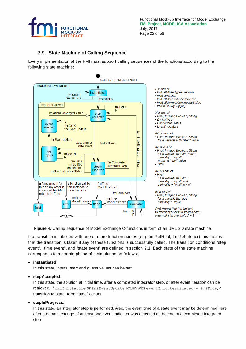
Figure 4: Calling sequence of Model Exchange C-functions in form of an UML 2.0 state machine.
If a transition is labelled with one or more function names (e.g. fmiGetReal, fmiGetInteger) this means
that the transition is taken if any of these functions is successfully called. The transition conditions "step
event", "time event", and "state event" are defined in section 2.1. Each state of the state machine
corresponds to a certain phase of a simulation as follows:
instantiated:
In this state, inputs, start and guess values can be set.
stepAccepted:
In this state, the solution at initial time, after a completed integrator step, or after event iteration can be
retrieved. If fmiInitialize or fmiEventUpdate return with eventInfo.terminated = fmiTrue, a
transition to state “terminated” occurs.
stepInProgress:
In this state, an integrator step is performed. Also, the event time of a state event may be determined here
after a domain change of at least one event indicator was detected at the end of a completed integrator
step.
Functional Mock-up Interface for Model Exchange
FMI Project, MODELICA Association
July, 2017
Page 23 of 56
setInputs:
Before starting with the event handling, changed (continuous or discrete) inputs have to be set.
eventPending:
In this state, at least one event is waiting to be processed by a call to fmiEventUpdate. Intermediate
results of the event iteration can be retrieved. If fmiEventUpdate returns with
eventInfo.iterationConverged = fmiTrue, then this state is left and the state machine continues in
state “retrieveSolution”.
terminated:
In this state, the solution at the final time of a simulation can be retrieved.
Note, that simulation backward in time cannot be performed with an FMU, at least not across event
times, because fmiEventUpdate can only compute the next discrete state, not the previous one.
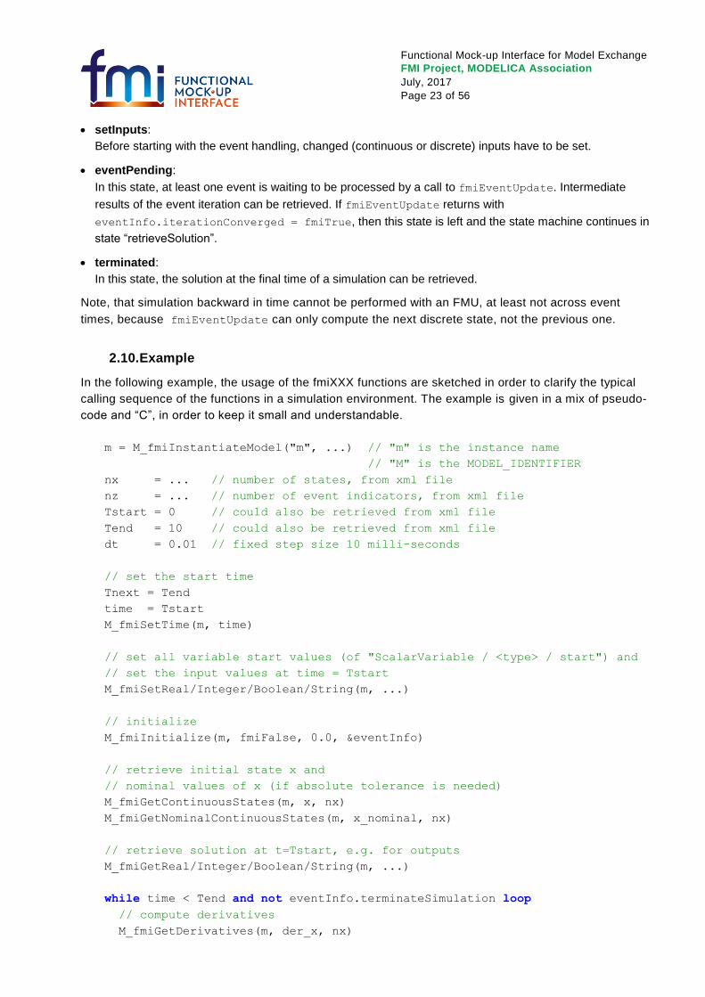
2.10. Example
In the following example, the usage of the fmiXXX functions are sketched in order to clarify the typical
calling sequence of the functions in a simulation environment. The example is given in a mix of pseudo-
code and “C”, in order to keep it small and understandable.
m = M_fmiInstantiateModel("m", ...) // "m" is the instance name
// "M" is the MODEL_IDENTIFIER
nx = ... // number of states, from xml file
nz = ... // number of event indicators, from xml file
Tstart = 0 // could also be retrieved from xml file
Tend = 10 // could also be retrieved from xml file
dt = 0.01 // fixed step size 10 milli-seconds
// set the start time
Tnext = Tend
time = Tstart
M_fmiSetTime(m, time)
// set all variable start values (of "ScalarVariable / <type> / start") and
// set the input values at time = Tstart
M_fmiSetReal/Integer/Boolean/String(m, ...)
// initialize
M_fmiInitialize(m, fmiFalse, 0.0, &eventInfo)
// retrieve initial state x and
// nominal values of x (if absolute tolerance is needed)
M_fmiGetContinuousStates(m, x, nx)
M_fmiGetNominalContinuousStates(m, x_nominal, nx)
// retrieve solution at t=Tstart, e.g. for outputs
M_fmiGetReal/Integer/Boolean/String(m, ...)
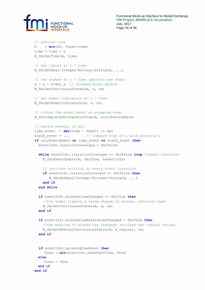
while time < Tend and not eventInfo.terminateSimulation loop
// compute derivatives
M_fmiGetDerivatives(m, der_x, nx)
Functional Mock-up Interface for Model Exchange
FMI Project, MODELICA Association
July, 2017
Page 24 of 56
// advance time
h = min(dt, Tnext-time)
time = time + h
M_fmiSetTime(m, time)
// set inputs at t = time
M_fmiSetReal/Integer/Boolean/String(m, ...)
// set states at t = time (perform one step)
x = x + h*der_x // forward Euler method
M_fmiSetContinuousStates(m, x, nx)
// get event indicators at t = time
M_fmiGetEventIndicators(m, z, nz)
// inform the model about an accepted step
M_fmiCompletedIntegratorStep(m, &callEventUpdate)
// handle events, if any
time_event = abs(time - Tnext) <= eps
state_event = ... // compare sign of z with previous z
if callEventUpdate or time_event or state_event then
eventInfo.iterationConverged = fmiFalse
while eventInfo.iterationConverged == fmiFalse loop //event iteration
M_fmiEventUpdate(m, fmiTrue, &eventInfo)
// retrieve solution at every event iteration
if eventInfo.iterationConverged == fmiFalse then
M_fmiGetReal/Integer/Boolean/String(m, ...)
end if
end while
if eventInfo.stateValuesChanged == fmiTrue then
//the model signals a value change of states, retrieve them
M_fmiGetContinuousStates(m, x, nx)
end if
if eventInfo.stateValueReferencesChanged = fmiTrue then
//the meaning of states has changed; retrieve new nominal values
M_fmiGetNominalContinuousStates(m, x_nominal, nx)
end if
if eventInfo.upcomingTimeEvent then
Tnext = min(eventInfo.nextEventTime, Tend)
else
Tnext = Tend
end if
end if
Functional Mock-up Interface for Model Exchange
FMI Project, MODELICA Association
July, 2017
Page 25 of 56
// Retrieve solution at t=time, e.g. for outputs
M_fmiGetReal/Integer/Boolean/String(m, ...)
end while
// terminate simulation and retrieve final values
M_fmiTerminate(m)
M_fmiGetReal/Integer/Boolean/String(m, ...)
// cleanup
M_fmiFreeModelInstance(m)
Above, errors are not handled. Typically, fmiXXX function calls are performed in the following way:
status = M_fmiGetDerivatives(m, der_x, nx);
if ( status == fmiDiscard ) goto DISCARD; // reduce step size and try again
if ( status == fmiError ) goto ERROR; // cleanup and stop simulation
if ( status == fmiFatal ) goto FATAL; // stop using the model
These if-clauses could also be collected together in a macro to simplify the code.
Functional Mock-up Interface for Model Exchange
FMI Project, MODELICA Association
July, 2017
Page 26 of 56
3. Model Description Schema
All information related to a model, with exception of the model equations, are stored in a text file in xml
format. Especially, the model variables and their attributes such as name, unit, default initial value etc.
are stored in this file. The structure of all such xml files is defined with the schema file
“fmiModelDescription.xsd”. This schema file utilizes the following helper schema files:
fmiBaseUnit.xsd
fmiType.xsd
fmiScalarVariable.xsd
In this section the schema files are described. The normative definition are the above mentioned schema
files5. Below, optional elements are marked with a “dashed” box. The required data types (like:
xs:normalizedString) are defined in the xml-schema standard: http://www.w3.org/TR/xmlschema-2/. The
types used in the fmi schema files are:
XML Description (http://www.w3.org/TR/xmlschema-2/) Mapping to C
xs:double IEEE double-precision 64-bit floating point type double
xs:int Integer number with maximum value 2147483647 and
minimum value -2147483648 (32 bit Integer)
int
xs:unsignedInt Integer number with maximum value 4294967295 and
minimum value 0 (unsigned 32 bit Integer)
unsigned int
xs:boolean Boolean number. Legal literals: false, true, 0, 1 char
xs:string Any number of characters char*
xs:normalizedString String without carriage return, line feed, and tab characters char*
xs:dateTime Date, time and time zone (for details see the link above).
Example: 2002-10-23T12:00:00Z
(noon on October 23, 2002, Greenwich Mean Time)
tool specific
The first line of an xml file must contain the encoding scheme of the xml-file, such as:
<?xml version="1.0" encoding="UTF-8"?>
A specific encoding scheme is not required by the fmi schema files. Typical schemes are "ISO-8859-1"
or “UTF-8”. The fmi schema files are stored in “UTF8”. Note, the definition of an encoding scheme is a
prerequisite, in order that the xml-file can contain letters outside of the 7 bit ANSI ASCII character set,
such as German umlauts, or Asian characters. If another encoding scheme as “UTF-8” is used, then the
non-ASCII characters in string variables need to be transformed to UTF8 when reading them from file,
because the FMI calling interface requires that strings are encoded in UTF8.
5 Note, the screenshots of this section have been generated from the schema files with the too l “Altova XMLSpy”
(www.altova.com). With the enterprise edition of XMLSpy it is possible to automatically generate C++, C# and Java code that
reads an xml-file of fmiModelDescription.xsd.
Functional Mock-up Interface for Model Exchange
FMI Project, MODELICA Association
July, 2017
Page 27 of 56
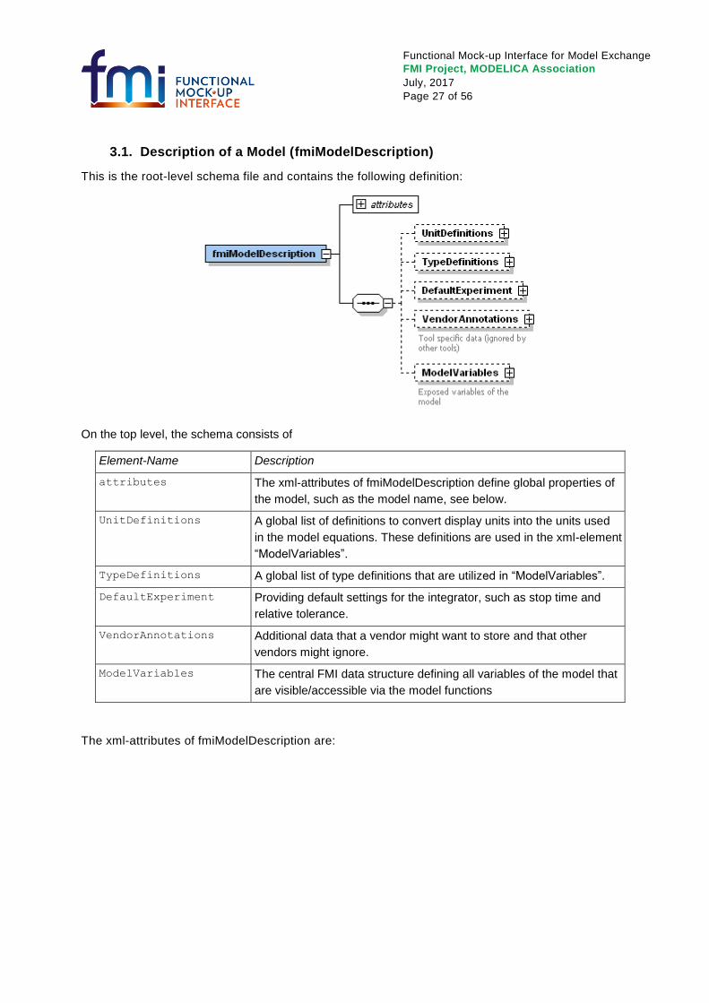
3.1. Description of a Model (fmiModelDescription)
This is the root-level schema file and contains the following definition:
On the top level, the schema consists of
Element-Name Description
attributes
The xml-attributes of fmiModelDescription define global properties of
the model, such as the model name, see below.
UnitDefinitions A global list of definitions to convert display units into the units used
in the model equations. These definitions are used in the xml-element
“ModelVariables”.
TypeDefinitions A global list of type definitions that are utilized in “ModelVariables”.
DefaultExperiment
Providing default settings for the integrator, such as stop time and
relative tolerance.
VendorAnnotations Additional data that a vendor might want to store and that other
vendors might ignore.
ModelVariables The central FMI data structure defining all variables of the model that
are visible/accessible via the model functions
The xml-attributes of fmiModelDescription are:
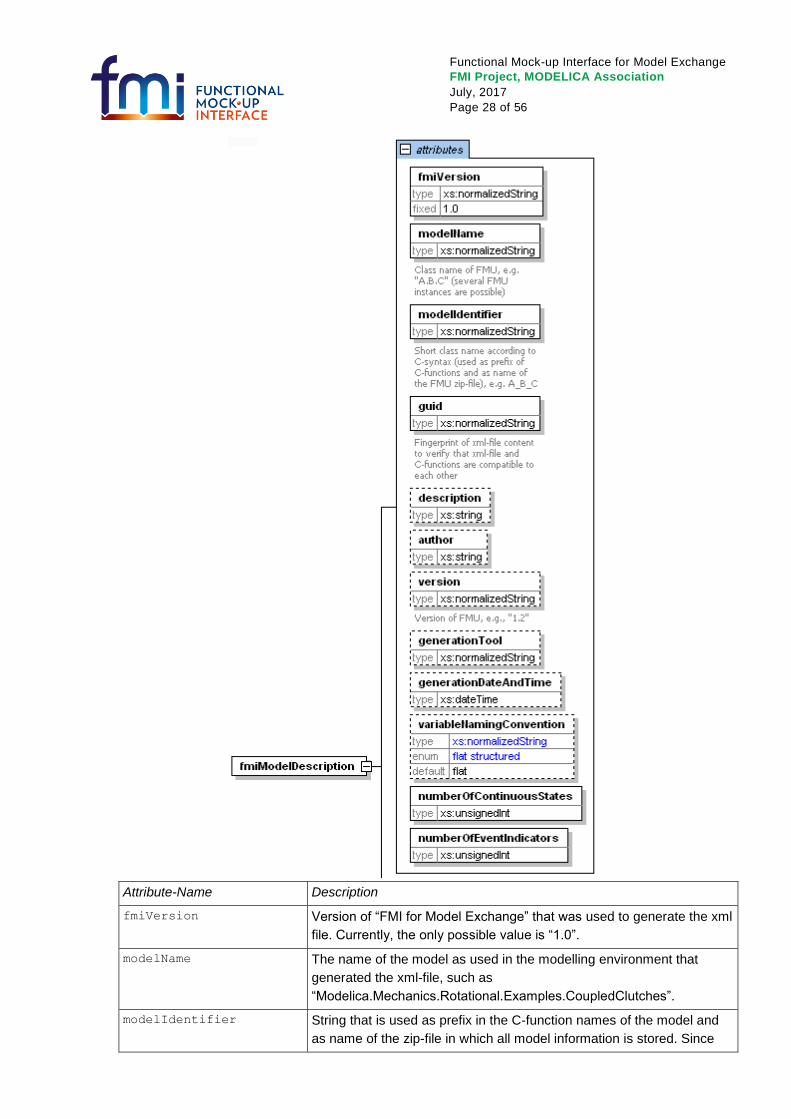
Functional Mock-up Interface for Model Exchange
FMI Project, MODELICA Association
July, 2017
Page 28 of 56
Attribute-Name Description
fmiVersion Version of “FMI for Model Exchange” that was used to generate the xml
file. Currently, the only possible value is “1.0”.
modelName The name of the model as used in the modelling environment that
generated the xml-file, such as
“Modelica.Mechanics.Rotational.Examples.CoupledClutches”.
modelIdentifier String that is used as prefix in the C-function names of the model and
as name of the zip-file in which all model information is stored. Since
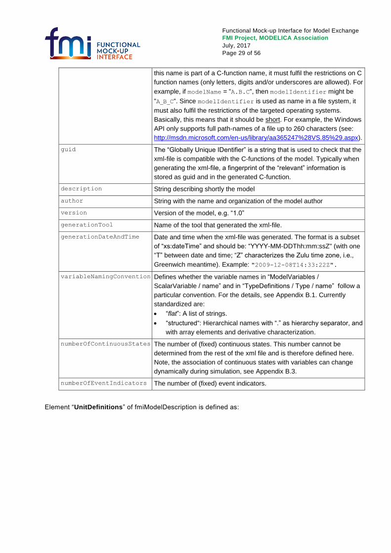
Functional Mock-up Interface for Model Exchange
FMI Project, MODELICA Association
July, 2017
Page 29 of 56
this name is part of a C-function name, it must fulfil the restrictions on C
function names (only letters, digits and/or underscores are allowed). For
example, if modelName = “A.B.C“, then modelIdentifier might be
“ABC“. Since modelIdentifier is used as name in a file system, it
must also fulfil the restrictions of the targeted operating systems.
Basically, this means that it should be short. For example, the Windows
API only supports full path-names of a file up to 260 characters (see:
http://msdn.microsoft.com/en-us/library/aa365247%28VS.85%29.aspx).
guid The “Globally Unique IDentifier” is a string that is used to check that the
xml-file is compatible with the C-functions of the model. Typically when
generating the xml-file, a fingerprint of the “relevant” information is
stored as guid and in the generated C-function.
description String describing shortly the model
author String with the name and organization of the model author
version Version of the model, e.g. “1.0”
generationTool Name of the tool that generated the xml-file.
generationDateAndTime Date and time when the xml-file was generated. The format is a subset
of “xs:dateTime” and should be: “YYYY-MM-DDThh:mm:ssZ" (with one
“T” between date and time; “Z” characterizes the Zulu time zone, i.e.,
Greenwich meantime). Example: "2009-12-08T14:33:22Z".
variableNamingConvention
Defines whether the variable names in “ModelVariables /
ScalarVariable / name” and in “TypeDefinitions / Type / name” follow a
particular convention. For the details, see Appendix B.1. Currently
standardized are:
“flat”: A list of strings.
“structured“: Hierarchical names with “.” as hierarchy separator, and
with array elements and derivative characterization.
numberOfContinuousStates The number of (fixed) continuous states. This number cannot be
determined from the rest of the xml file and is therefore defined here.
Note, the association of continuous states with variables can change
dynamically during simulation, see Appendix B.3.
numberOfEventIndicators The number of (fixed) event indicators.
Element “UnitDefinitions” of fmiModelDescription is defined as:
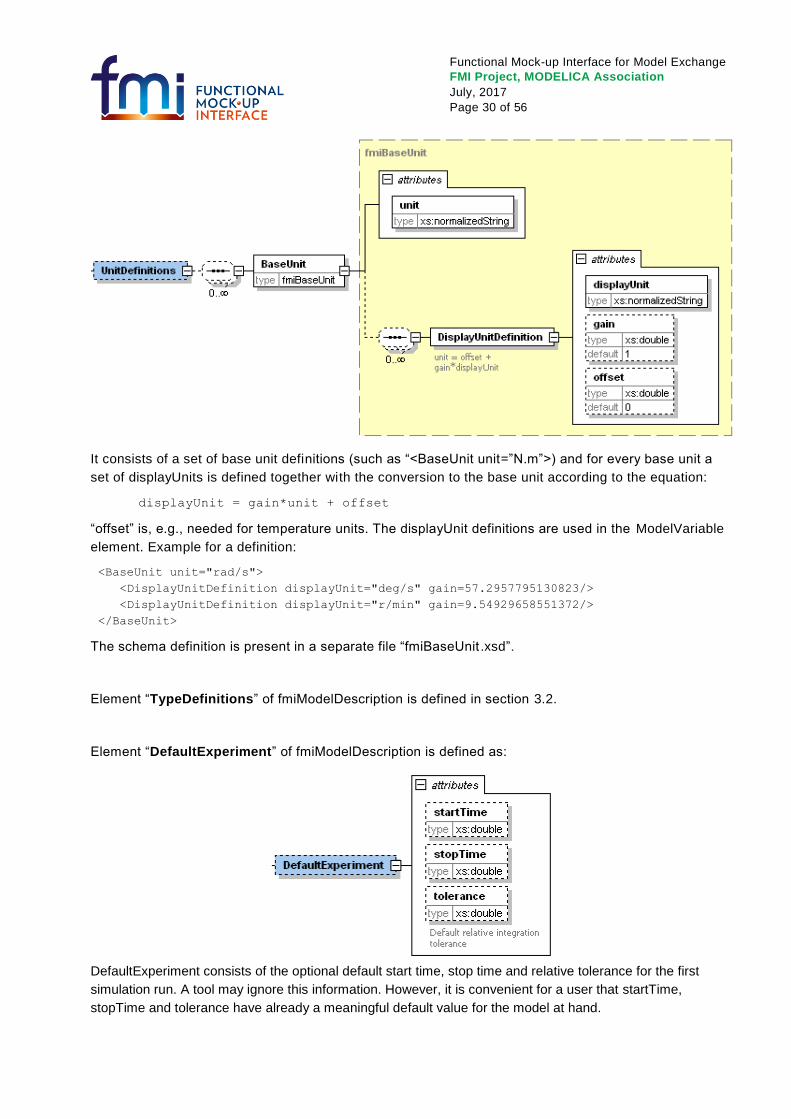
Functional Mock-up Interface for Model Exchange
FMI Project, MODELICA Association
July, 2017
Page 30 of 56
It consists of a set of base unit definitions (such as “<BaseUnit unit=”N.m”>) and for every base unit a
set of displayUnits is defined together with the conversion to the base unit according to the equation:
displayUnit = gain*unit + offset
“offset” is, e.g., needed for temperature units. The displayUnit definitions are used in the ModelVariable
element. Example for a definition:
<BaseUnit unit="rad/s">
<DisplayUnitDefinition displayUnit="deg/s" gain=57.2957795130823/>
<DisplayUnitDefinition displayUnit="r/min" gain=9.54929658551372/>
</BaseUnit>
The schema definition is present in a separate file “fmiBaseUnit .xsd”.
Element “TypeDefinitions” of fmiModelDescription is defined in section 3.2.
Element “DefaultExperiment” of fmiModelDescription is defined as:
DefaultExperiment consists of the optional default start time, stop time and relative tolerance for the first
simulation run. A tool may ignore this information. However, it is convenient for a user that startTime,
stopTime and tolerance have already a meaningful default value for the model at hand.
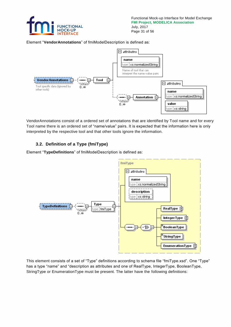
Functional Mock-up Interface for Model Exchange
FMI Project, MODELICA Association
July, 2017
Page 31 of 56
Element “VendorAnnotations” of fmiModelDescription is defined as:
VendorAnnotations consist of a ordered set of annotations that are identified by Tool name and for every
Tool name there is an ordered set of “name/value” pairs. It is expected that the information here is only
interpreted by the respective tool and that other tools ignore the information.
3.2. Definition of a Type (fmiType)
Element “TypeDefinitions” of fmiModelDescription is defined as:
This element consists of a set of “Type” definitions according to schema file “fmiType.xsd”. One “Type”
has a type “name” and “description as attributes and one of RealType, IntegerType, BooleanType,
StringType or EnumerationType must be present. The latter have the following definitions:
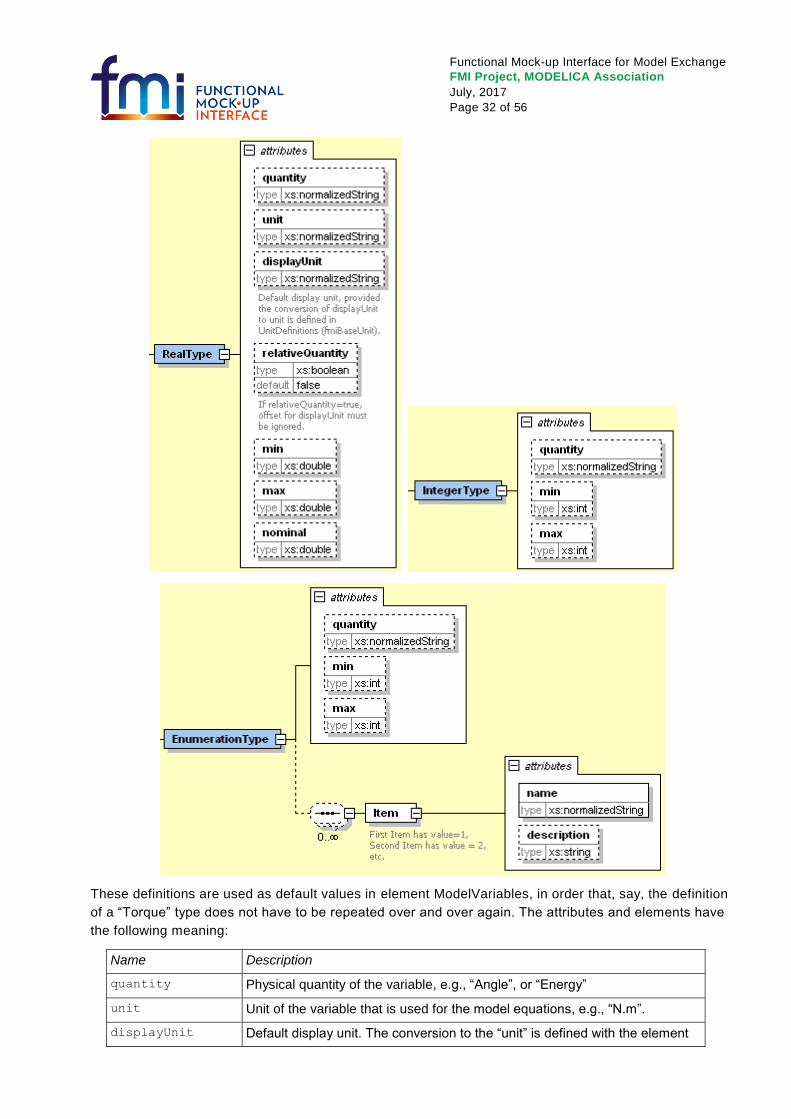
Functional Mock-up Interface for Model Exchange
FMI Project, MODELICA Association
July, 2017
Page 32 of 56
These definitions are used as default values in element ModelVariables, in order that, say, the definition
of a “Torque” type does not have to be repeated over and over again. The attributes and elements have
the following meaning:
Name Description
quantity Physical quantity of the variable, e.g., “Angle”, or “Energy”
unit Unit of the variable that is used for the model equations, e.g., “N.m”.
displayUnit Default display unit. The conversion to the “unit” is defined with the element
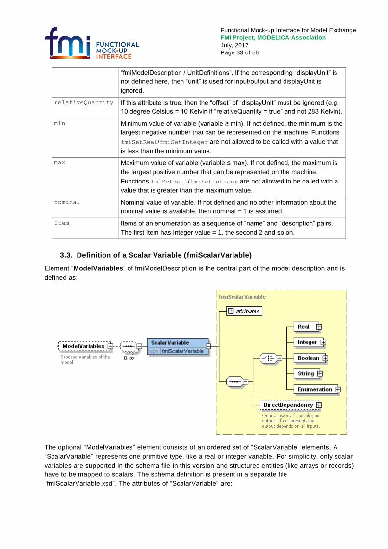
Functional Mock-up Interface for Model Exchange
FMI Project, MODELICA Association
July, 2017
Page 33 of 56
“fmiModelDescription / UnitDefinitions”. If the corresponding “displayUnit” is
not defined here, then “unit” is used for input/output and displayUnit is
ignored.
relativeQuantity If this attribute is true, then the “offset” of “displayUnit” must be ignored (e.g.
10 degree Celsius = 10 Kelvin if “relativeQuantity = true” and not 283 Kelvin).
min Minimum value of variable (variable ≥ min). If not defined, the minimum is the
largest negative number that can be represented on the machine. Functions
fmiSetReal/fmiSetInteger are not allowed to be called with a value that
is less than the minimum value.
max Maximum value of variable (variable ≤ max). If not defined, the maximum is
the largest positive number that can be represented on the machine.
Functions fmiSetReal/fmiSetInteger are not allowed to be called with a
value that is greater than the maximum value.
nominal Nominal value of variable. If not defined and no other information about the
nominal value is available, then nominal = 1 is assumed.
Item Items of an enumeration as a sequence of “name” and “description” pairs.
The first Item has Integer value = 1, the second 2 and so on.
3.3. Definition of a Scalar Variable (fmiScalarVariable)
Element “ModelVariables” of fmiModelDescription is the central part of the model description and is
defined as:
The optional “ModelVariables” element consists of an ordered set of “ScalarVariable” elements. A
“ScalarVariable” represents one primitive type, like a real or integer variable. For simplicity, only scalar
variables are supported in the schema file in this version and structured entities (like arrays or records)
have to be mapped to scalars. The schema definition is present in a separate file
“fmiScalarVariable.xsd”. The attributes of “ScalarVariable” are:
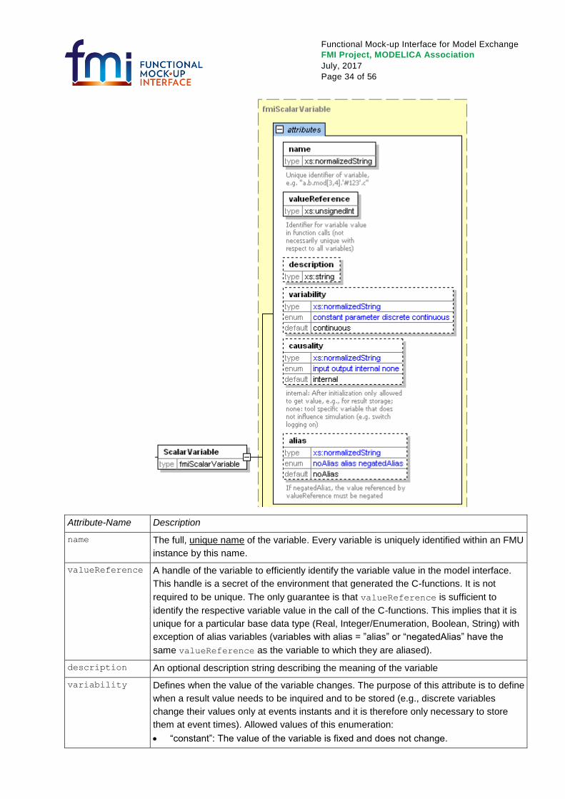
Functional Mock-up Interface for Model Exchange
FMI Project, MODELICA Association
July, 2017
Page 34 of 56
Attribute-Name Description
name
The full, unique name of the variable. Every variable is uniquely identified within an FMU
instance by this name.
valueReference A handle of the variable to efficiently identify the variable value in the model interface.
This handle is a secret of the environment that generated the C-functions. It is not
required to be unique. The only guarantee is that valueReference is sufficient to
identify the respective variable value in the call of the C-functions. This implies that it is
unique for a particular base data type (Real, Integer/Enumeration, Boolean, String) with
exception of alias variables (variables with alias = ”alias” or “negatedAlias” have the
same valueReference as the variable to which they are aliased).
description An optional description string describing the meaning of the variable
variability Defines when the value of the variable changes. The purpose of this attribute is to define
when a result value needs to be inquired and to be stored (e.g., discrete variables
change their values only at events instants and it is therefore only necessary to store
them at event times). Allowed values of this enumeration:
“constant”: The value of the variable is fixed and does not change.
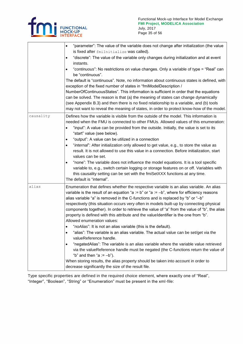
Functional Mock-up Interface for Model Exchange
FMI Project, MODELICA Association
July, 2017
Page 35 of 56
“parameter”: The value of the variable does not change after initialization (the value
is fixed after fmiInitialize was called).
“discrete”: The value of the variable only changes during initialization and at event
instants.
“continuous”: No restrictions on value changes. Only a variable of type = “Real” can
be “continuous”.
The default is “continuous”. Note, no information about continuous states is defined, with
exception of the fixed number of states in “fmiModelDescription /
NumberOfContinuousStates”. This information is sufficient in order that the equations
can be solved. The reason is that (a) the meaning of states can change dynamically
(see Appendix B.3) and then there is no fixed relationship to a variable, and (b) tools
may not want to reveal the meaning of states, in order to protect know-how of the model.
causality Defines how the variable is visible from the outside of the model. This information is
needed when the FMU is connected to other FMUs. Allowed values of this enumeration:
“input”: A value can be provided from the outside. Initially, the value is set to its
“start” value (see below).
“output”: A value can be utilized in a connection
“internal”: After initialization only allowed to get value, e.g., to store the value as
result. It is not allowed to use this value in a connection. Before initialization, start
values can be set.
“none”: The variable does not influence the model equations. It is a tool specific
variable to, e.g., switch certain logging or storage features on or off. Variables with
this causality setting can be set with the fmiSetXXX functions at any time.
The default is “internal”.
alias Enumeration that defines whether the respective variable is an alias variable. An alias
variable is the result of an equation “a := b” or “a := –b”, where for efficiency reasons
alias variable “a” is removed in the C-functions and is replaced by “b” or “–b”
respectively (this situation occurs very often in models built-up by connecting physical
components together). In order to retrieve the value of “a” from the value of “b”, the alias
property is defined with this attribute and the valueIdentifier is the one from “b”.
Allowed enumeration values:
“noAlias”: It is not an alias variable (this is the default).
“alias”: The variable is an alias variable. The actual value can be set/get via the
valueReference handle.
“negatedAlias”: The variable is an alias variable where the variable value retrieved
via the valueReference handle must be negated (the C-functions return the value of
“b” and then “a := –b”).
When storing results, the alias property should be taken into account in order to
decrease significantly the size of the result file.
Type specific properties are defined in the required choice element, where exactly one of “Real”,
“Integer”, “Boolean”, “String” or “Enumeration” must be present in the xml -file:
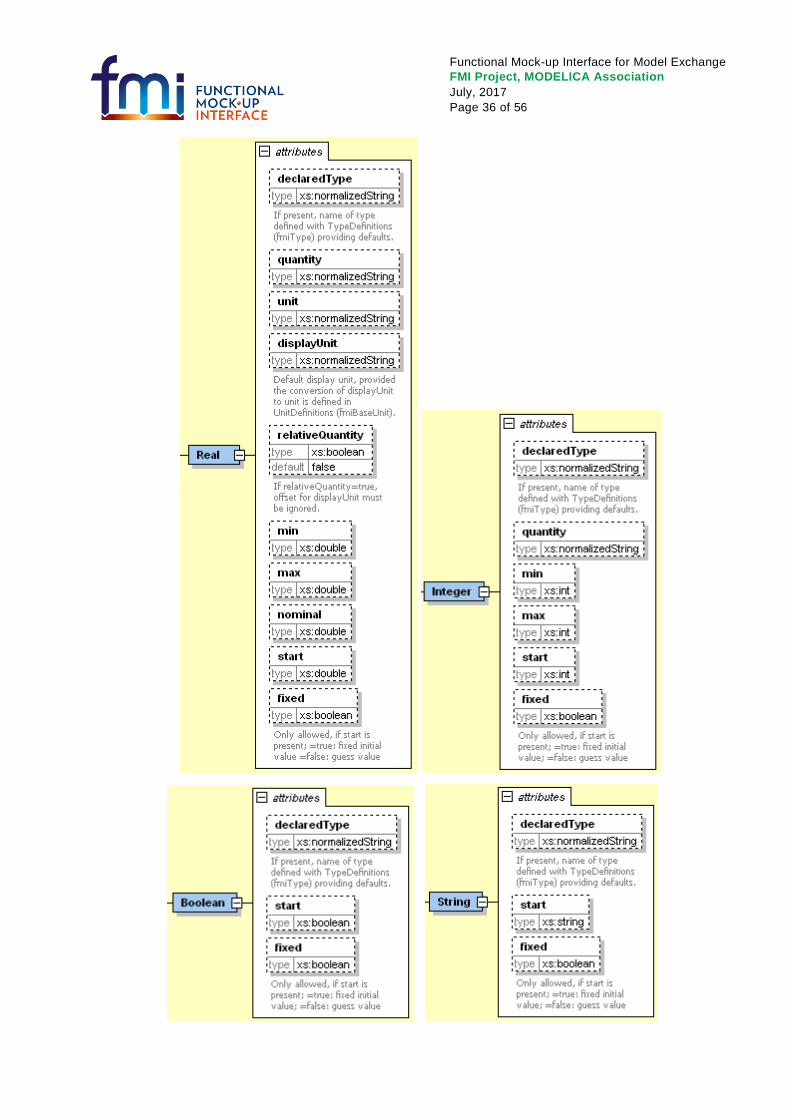
Functional Mock-up Interface for Model Exchange
FMI Project, MODELICA Association
July, 2017
Page 36 of 56
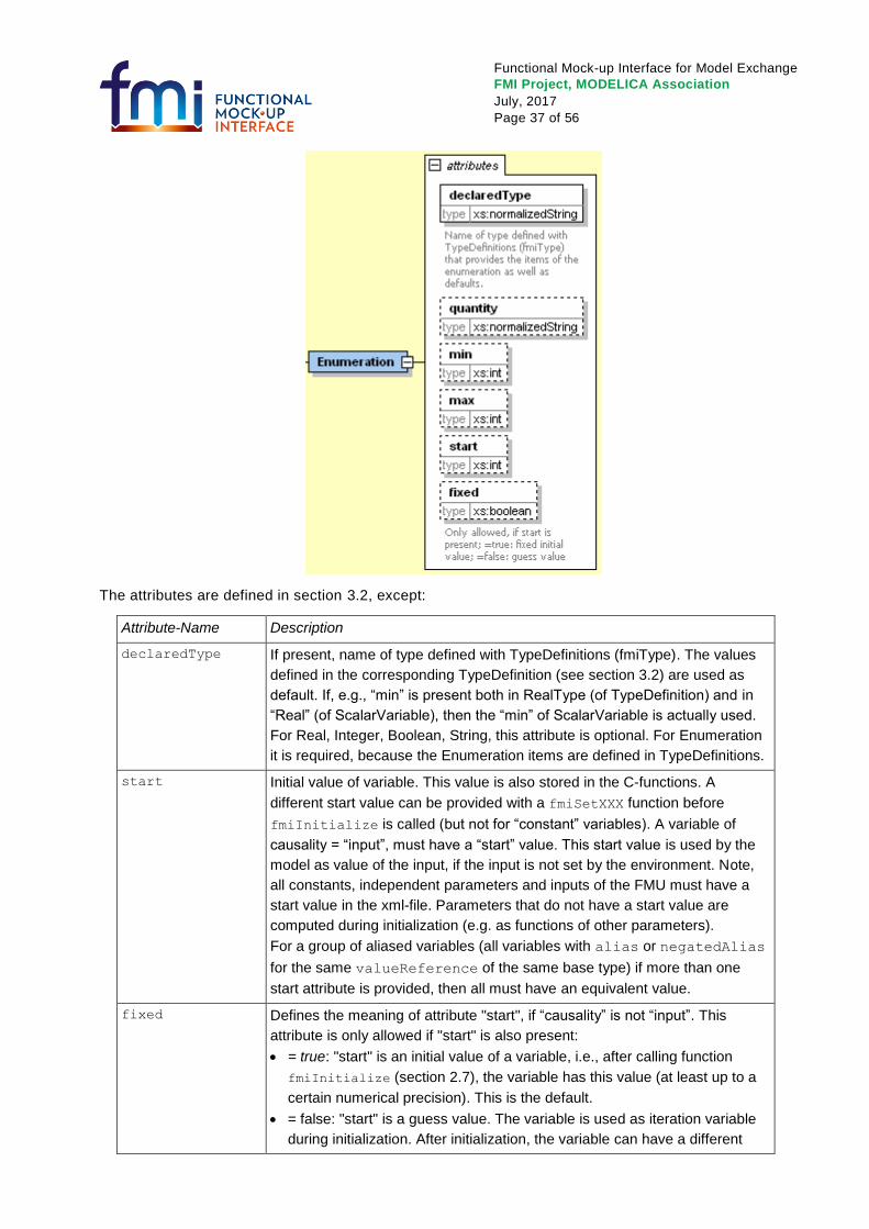
Functional Mock-up Interface for Model Exchange
FMI Project, MODELICA Association
July, 2017
Page 37 of 56
The attributes are defined in section 3.2, except:
Attribute-Name Description
declaredType If present, name of type defined with TypeDefinitions (fmiType). The values
defined in the corresponding TypeDefinition (see section 3.2) are used as
default. If, e.g., “min” is present both in RealType (of TypeDefinition) and in
“Real” (of ScalarVariable), then the “min” of ScalarVariable is actually used.
For Real, Integer, Boolean, String, this attribute is optional. For Enumeration
it is required, because the Enumeration items are defined in TypeDefinitions.
start Initial value of variable. This value is also stored in the C-functions. A
different start value can be provided with a fmiSetXXX function before
fmiInitialize is called (but not for “constant” variables). A variable of
causality = “input”, must have a “start” value. This start value is used by the
model as value of the input, if the input is not set by the environment. Note,
all constants, independent parameters and inputs of the FMU must have a
start value in the xml-file. Parameters that do not have a start value are
computed during initialization (e.g. as functions of other parameters).
For a group of aliased variables (all variables with alias or negatedAlias
for the same valueReference of the same base type) if more than one
start attribute is provided, then all must have an equivalent value.
fixed Defines the meaning of attribute "start", if “causality” is not “input”. This
attribute is only allowed if "start" is also present:
= true: "start" is an initial value of a variable, i.e., after calling function
fmiInitialize (section 2.7), the variable has this value (at least up to a
certain numerical precision). This is the default.
= false: "start" is a guess value. The variable is used as iteration variable
during initialization. After initialization, the variable can have a different
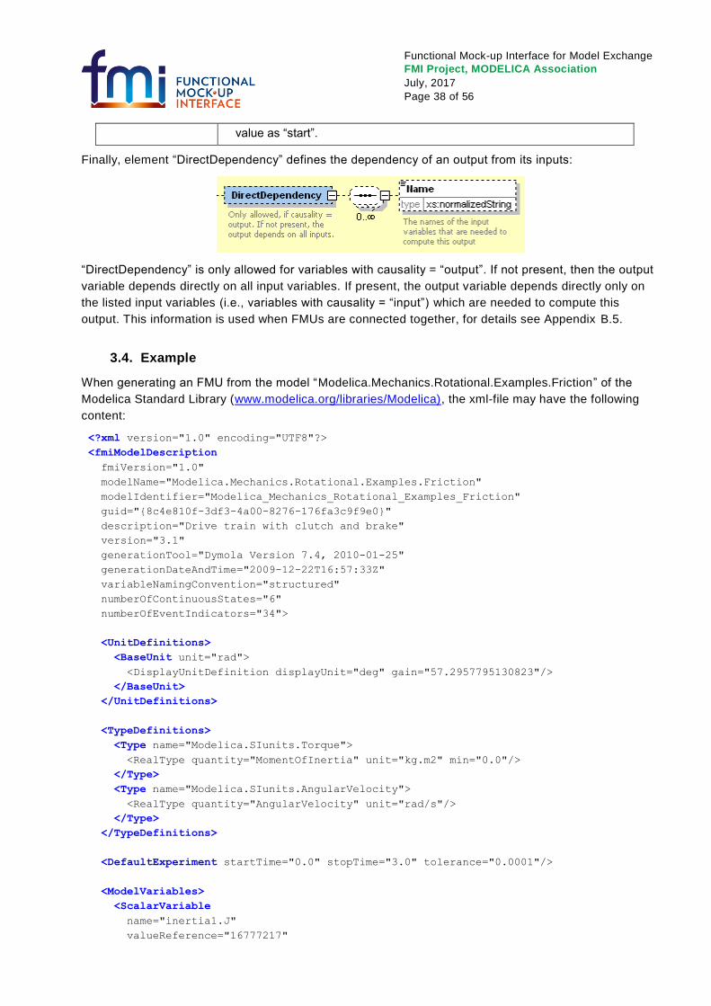
Functional Mock-up Interface for Model Exchange
FMI Project, MODELICA Association
July, 2017
Page 38 of 56
value as “start”.
Finally, element “DirectDependency” defines the dependency of an output from its inputs:
“DirectDependency” is only allowed for variables with causality = “output”. If not present, then the output
variable depends directly on all input variables. If present, the output variable depends directly only on
the listed input variables (i.e., variables with causality = “input”) which are needed to compute this
output. This information is used when FMUs are connected together, for details see Appendix B.5.
3.4. Example
When generating an FMU from the model “Modelica.Mechanics.Rotational.Examples.Friction” of the
Modelica Standard Library (www.modelica.org/libraries/Modelica), the xml-file may have the following
content:
<?xml version="1.0" encoding="UTF8"?>
<fmiModelDescription
fmiVersion="1.0"
modelName="Modelica.Mechanics.Rotational.Examples.Friction"
modelIdentifier="Modelica_Mechanics_Rotational_Examples_Friction"
guid="{8c4e810f-3df3-4a00-8276-176fa3c9f9e0}"
description="Drive train with clutch and brake"
version="3.1"
generationTool="Dymola Version 7.4, 2010-01-25"
generationDateAndTime="2009-12-22T16:57:33Z"
variableNamingConvention="structured"
numberOfContinuousStates="6"
numberOfEventIndicators="34">
<UnitDefinitions>
<BaseUnit unit="rad">
<DisplayUnitDefinition displayUnit="deg" gain="57.2957795130823"/>
</BaseUnit>
</UnitDefinitions>
<TypeDefinitions>
<Type name="Modelica.SIunits.Torque">
<RealType quantity="MomentOfInertia" unit="kg.m2" min="0.0"/>
</Type>
<Type name="Modelica.SIunits.AngularVelocity">
<RealType quantity="AngularVelocity" unit="rad/s"/>
</Type>
</TypeDefinitions>
<DefaultExperiment startTime="0.0" stopTime="3.0" tolerance="0.0001"/>
<ModelVariables>
<ScalarVariable
name="inertia1.J"
valueReference="16777217"

Functional Mock-up Interface for Model Exchange
FMI Project, MODELICA Association
July, 2017
Page 39 of 56
description="Moment of inertia"
variability="parameter">
<Real declaredType="Modelica.SIunits.Torque" start="1"/>
</ScalarVariable>
<ScalarVariable
name="inertia1.w"
valueReference="33554433"
description="Absolute angular velocity of component (= der(phi))">
<Real declaredType="Modelica.SIunits.AngularVelocity" start="100"/>
</ScalarVariable>
...
</ModelVariables>
</fmiModelDescription>
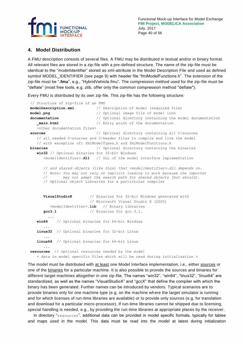
Functional Mock-up Interface for Model Exchange
FMI Project, MODELICA Association
July, 2017
Page 40 of 56
4. Model Distribution
A FMU description consists of several files. A FMU may be distributed in textual and/or in binary format.
All relevant files are stored in a zip-file with a pre-defined structure. The name of the zip-file must be
identical to the “modelIdentifier” stored as xml-attribute in the Model Description File and used as defined
symbol MODEL_IDENTIFIER (see page 9) with header file “fmiModelFunctions.h”. The extension of the
zip-file must be “.fmu”, e.g., “HybridVehicle.fmu”. The compression method used for the zip-file must be
“deflate” (most free tools, e.g. zlib, offer only the common compression method "deflate").
Every FMU is distributed by its own zip-file. This zip-file has the following structure:
// Structure of zip-file of an FMU
modelDescription.xml // Description of model (required file)
model.png // Optional image file of model icon
documentation // Optional directory containing the model documentation
_main.html // Entry point of the documentation
<other documentation files>
sources // Optional directory containing all C-sources
// all needed C-sources and C-header files to compile and link the model
// with exception of: fmiModelTypes.h and fmiModelFunctions.h
binaries // Optional directory containing the binaries
win32 // Optional binaries for 32-bit Windows
<modelIdentifier>.dll // DLL of the model interface implementation
// and shared objects (like DLLs) that <modelIdentifier>.dll depends on.
// Note: You may not rely on implicit loading to work because the importer
// may not adapt the search path for shared objects [but should].
// Optional object Libraries for a partictular compiler
VisualStudio8 // Binaries for 32-bit Windows generated with
// Microsoft Visual Studio 8 (2005)
<modelIdentifier>.lib // Binary libraries
gcc3.1 // Binaries for gcc 3.1.
...
win64 // Optional binaries for 64-bit Windows
...
linux32 // Optional binaries for 32-bit Linux
...
linux64 // Optional binaries for 64-bit Linux
...
resources // Optional resources needed by the model
< data in model specific files which will be read during initialization >
The model must be distributed with at least one Model Interface implementation, i.e., either sources or
one of the binaries for a particular machine. It is also possible to provide the sources and binaries for
different target machines altogether in one zip-file. The names “win32”, “win64”, “linux32”, “linux64” are
standardized, as well as the names “VisualStudioX” and “gccX” that define the compiler with which the
binary has been generated. Further names can be introduced by vendors. Typical scenarios are to
provide binaries only for one machine type (e.g. on the machine where the target simulator is running
and for which licenses of run-time libraries are available) or to provide only sources (e.g. for translation
and download for a particular micro-processor). If run-time libraries cannot be shipped due to licensing,
special handling is needed, e.g., by providing the run-time libraries at appropriate places by the receiver.
In directory “resources”, additional data can be provided in model specific formats, typically for tables
and maps used in the model. This data must be read into the model at latest during initialization

Functional Mock-up Interface for Model Exchange
FMI Project, MODELICA Association
July, 2017
Page 41 of 56
(“fmiInitialize”). The actual file names in the zip-file to access the data files can either be hard-coded in
the generated model functions, or the file names can be provided as string parameters via the
“fmiSetString” function.
Note, the header files fmiModelTypes.h and fmiModelFunctions.h are not included in the FMU due
to the following reasons:
fmiModelTypes.h makes no sense in the “sources” directory, because if sources are provided, then the
target simulator defines this header file and not the FMU.
This header file is not included in the “binaries” directory, because it is implicitly defined by the platform
directory (e.g. win32 for 32-bit machine or linux64 for 64-bit machine). Furthermore, the version that was
used to construct the FMU can also be inquired via function fmiGetModelTypesPlatform().
fmiModelFunctions.h is not needed in the “sources” directory, because it is implicitly defined by
atttribute fmiVersion in file modelDescription.xml. Furthermore, in order that the C-compiler can
check for consistent function arguments, the header file from the target simulator should be used when
compiling the C-sources. It would therefore be counter productive (unsafe), if this header file would be
present.
This header file is not included in the “binaries” directory, since this header file was already utilized to
build the target simulator executable. Via attribute fmiVersion in file modelDescription.xml or via
function call fmiGetVersion() the version number of this header file used to construct the FMU can be
deduced.
Functional Mock-up Interface for Model Exchange
FMI Project, MODELICA Association
July, 2017
Page 42 of 56
5. Literature
AMESim: www.lmsintl.com/
AUTOSAR: www.autosar.org.
Blochwitz T., Kurzbach G., Neidhold T. (2008): An External Model Interface for Modelica. 6-th International
Modelica Conference, Bielefeld 2008.
www.modelica.org/events/modelica2008/Proceedings/sessions/session5f.pdf
Dymola: www.dynasim.se.
Elmqvist (1978): A Structured Model Language for Large Continuous Systems. PhD Dissertation, Lund
Institute of Technology. CODEN: LUTFD2/(TFRT-1015)/1-226/(1978).
www.control.lth.se/database/publications/article.pike?artkey=elm78dis
EXITE: www.extessy.com
Modelica (2009): Modelica, A Unified Object-Oriented Language for Physical Systems Modelling.
Language Specification, Version 3.1. May 27th, 2009.
www.modelica.org/documents/ModelicaSpec31.pdf
MODELISAR Glossary (2009): MODELISAR WP2 Glossary and Abbreviations. Version 1.0, June 9, 2009.
Otter M. (1999): Objektorientierte Modellierung Physikalischer Systeme, Teil 4. at –
Automatisierungstechnik, April, pp. A13-A16.
Otter M., Elmqvist H. (1995): The DSblock model interface for exchanging model components.
Proceedings of EUROSIM '95 Simulation Congress, pp. 505-510, Sept. 11-15, Vienna.
Silver: www.qtronic.de/de/silver.html
Simpack: www.simpack.com
SimulationX: www.simulationx.com.
Tarjan R.E. (1972): Depth First Search and Linear Graph Algorithms. SIAM J. Comp., 1, pp. 146-160.
XML: www.w3.org/XML, en.wikipedia.org/wiki/Xml

Functional Mock-up Interface for Model Exchange
FMI Project, MODELICA Association
July, 2017
Page 43 of 56
Appendix A Contributors
A.1 Version 1.0
The Functional Mock-up Interface subproject inside MODELISAR was initiated and organized by
Daimler AG. The development of version 1.0 was performed within WP200 of the MODELISAR ITEA2
project, organized by the WP200 work package leader Dietmar Neumerkel (Daimler). The subgroup “FMI
for Model Exchange” was headed by Martin Otter (DLR-RM). The essential part of the design of this
version was performed by (alphabetical list):
Torsten Blochwitz, ITI, Germany
Hilding Elmqvist, Dassault Systèmes (Dynasim), Sweden
Andreas Junghanns, QTronic, Germany
Jakob Mauss, QTronic, Germany
Hans Olsson, Dassault Systèmes (Dynasim), Sweden
Martin Otter, DLR-RM, Germany.
This version was evaluated with prototypes implemented for (alphabetical list):
Dymola by Peter Nilsson, Dan Henriksson, Carl Fredrik Abelson, and Sven Erik Mattson,
Dassault Systèmes (Dynasim),
JModelica.org by Tove Bergdahl, Modelon AB,
Silver by Andreas Junghanns, and Jakob Mauss, QTronic.
These prototypes have been used to refine the design of “FMI for Model Exchange”.
The following MODELISAR partners participated at FMI design meetings and contributed to the
discussion (alphabetical list):
Ingrid Bausch-Gall, Bausch-Gall GmbH, Munich, Germany
Torsten Blochwitz, ITI GmbH, Dresden, Germany
Alex Eichberger, SIMPACK AG, Gilching, Germany
Hilding Elmqvist, Dassault Systèmes (Dynasim), Lund, Sweden
Andreas Junghanns, QTronic GmbH, Berlin, Germany
Rainer Keppler, SIMPACK AG, Gilching, Germany
Gerd Kurzbach, ITI GmbH, Dresden, Germany
Carsten Kübler, TWT, Germany
Jakob Mauss, QTronic GmbH, Berlin, Germany
Johannes Mezger, TWT, Germany
Thomas Neidhold, ITI GmbH, Dresden, Germany
Dietmar Neumerkel, Daimler AG, Stuttgart, Germany
Peter Nilsson, Dassault Systèmes (Dynasim), Lund, Sweden
Hans Olsson, Dassault Systèmes (Dynasim), Lund, Sweden
Martin Otter, German Aerospace Center (DLR), Oberpfaffenhofen, Germany
Antoine Viel, LMS International (Imagine), Roanne, France
Daniel Weil, Dassault Systèmes, Grenoble, France
The following people outside of the MODELISAR consortium contributed with comments:
Johan Akesson, Lund University, Lund, Sweden
Joel Andersson, KU Leuven, The Netherlands
Roberto Parrotto, Politecnico di Milano, Italy
Functional Mock-up Interface for Model Exchange
FMI Project, MODELICA Association
July, 2017
Page 44 of 56
Appendix B Implementation Issues
In this section some details to implement the Model Exchange Interface are discussed.
B.1 Variable Naming Conventions
With attribute “variableNamingConvention” of element “fmiModelDescription”, the convention is defined
how the ScalarVariable.names have been constructed. If this information is known, the environment may
be able to represent the names in a better way (e.g. as tree and not as a linear list).
In the following definitions, the EBNF is used:
= production rule
[ ] optional
{ } repeat zero or more times
| or
The following conventions for scalar names are defined:
variableNamingConvention = “flat”
name = any member of the source character set // no hierarchy
The names are an ordered set that might be represented in a drop down menu as a list of strings.
variableNamingConvention = “structured”
Structured names are hierarchical using “.” as a separator between hierarchies. A name consists of “_”,
letters and digits or may consist of any characters enclosed in single apostrophes. A name may identify
an array element on every hierarchical level using “[...]” to identify the respective array index. A
derivative of a variable is defined with “der(name)” for the first time derivative and “der(name,N)” for
the N-th derivative. Examples:
vehicle.engine.speed
resistor12.u
v_min
robot.axis.′motor #234′
der(pipe[3,4].T[14],2) // second time derivative of pipe[3,4].T[14]
The precise syntax is:
name = identifier | "der(" identifier [, unsignedInteger ] ")"
identifier = B-name [ arrayIndices ] {"." B-name [ arrayIndices ] }
B-name = nondigit { digit | nondigit } | Q-name
nondigit = "_" | letters "a" to "z" | letters "A" to "Z"
digit = "0" | "1" | "2" | "3" | "4" | "5" | "6" | "7" | "8" | "9"
Q-name = "’" ( Q-char | escape ) { Q-char | escape } "’"
Q-char = any member of the source character set except
single-quote "’", and backslash "\"
escape = "\’" | "\"" | "\?" | "\\" | "\a" | "\b" |
"\f" | "\n" | "\r" | "\t" | "\v"
arrayIndices = "[" unsignedInteger {, unsignedInteger} "]"
unsignedInteger = digit { digit }
The tree of names is mapped to an ordered list of ScalarVariable .name’s in depth-first order. Example:
vehicle
transmission
Functional Mock-up Interface for Model Exchange
FMI Project, MODELICA Association
July, 2017
Page 45 of 56
ratio
outputSpeed
engine
inputSpeed
temperature
is mapped to the following list of ScalarVariable.name’s:
vehicle.transmission.ratio
vehicle.transmission.outputSpeed
vehicle.engine.inputSpeed
vehicle.engine.temperature
All array elements are given in a consecutive sequence of ScalarVariables. For example, the vector
“centerOfMass” in body “arm1” is mapped to the following ScalarVariables:
robot.arm1.centerOfMass[1]
robot.arm1.centerOfMass[2]
robot.arm2.centerOfMass[3]
It might be that not all elements of an array are present. If they are present, they are given in
consecutive order in the xml file.
B.2 Event Detection
An event is always triggered from the environment in which the FMU is called (so it is not triggered
inside the FMU). Typically, this is performed in the following:
1. The integration period is limited by the time event Tnext(ti-1) defined at the last event instant ti-1
(return argument eventInfo.nextEventTime of fmiEventUpdate), so the integrator integrates
from the previous event instant at most up to t = Tnext(ti-1). The integration step is thereby
adapted for the last step, so that it reaches Tnext exactly. If Tnext is reached, an event is triggered,
i.e., fmiEventUpdate is called.
2. The event indicators zj(t) are inspected after every completed integrator step. When the domain
of zj at this time instant is different to the domain from the last completed integrator step, an
iteration procedure is started to find the time instant ti (up to a certain precision), at which the
domain is changing. Then, an event is triggered, i.e., fmiEventUpdate is called.
3. At every completed integrator step, fmiCompletedIntegratorStep is called. When this
function returns with callEventUpdate = fmiTrue, an event is triggered, i.e., function
fmiEventUpdate is called.
It can happen that the conditions above lead to event times that are close together. Assume that n
potential event time instants t1, t2, t3, ..., tn (with t1 ≤ t2 ≤ t3 ≤ ... ≤ tn) are determined according to these
conditions (e.g., due to a time event, a step event, and domain changes of several event indicators) and
that these time instants are close together, e.g. tn - t1 ≤ 100·ε (where ε is the machine precision, which is
typically in the order of 10-16). For efficiency reasons it is then usually best to only trigger one event at t =
tn. Whether this is performed and if yes, which time range is used, is specific to the respective simulation
environment where the model is used.
State event detection leads to particular difficulties. One issue is that available integrators define state
events by the “zero crossing” of variables, whereas the Model Exchange Interface defines state events by
“domain changes”. The difference is that the “zero crossing” approach requires, that the event indicator
variables are non-zero after initialization and after restart of an event. However, this condition cannot be
guaranteed by a model. A related issue is that event handling may change the way a model is computed,
e.g., solving different linear equation systems before and after an event, as it is the case for friction elements
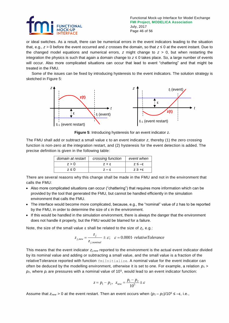
Functional Mock-up Interface for Model Exchange
FMI Project, MODELICA Association
July, 2017
Page 46 of 56
or ideal switches. As a result, there can be numerical errors in the event indicators leading to the situation
that, e.g., z > 0 before the event occurred and z crosses the domain, so that z ≤ 0 at the event instant. Due to
the changed model equations and numerical errors, z might change to z > 0, but when restarting the
integration the physics is such that again a domain change to z ≤ 0 takes place. So, a large number of events
will occur. Also more complicated situations can occur that lead to event “chattering” and that might be
treated in the FMU.
Some of the issues can be fixed by introducing hysteresis to the event indicators. The solution strategy is
sketched in Figure 5:
Figure 5: Introducing hysteresis for an event indicator z.
The FMU shall add or subtract a small value ε to an event indicator z, thereby (1) the zero crossing
function is non-zero at the integration restart, and (2) hysteresis for the event detection is added. The
precise definition is given in the following table:
domain at restart crossing function event when
z > 0 z + ε z ≤ –ε
z ≤ 0 z – ε z ≥ +ε
There are several reasons why this change shall be made in the FMU and not in the environment that
calls the FMU:
Also more complicated situations can occur (“chattering”) that requires more information which can be
provided by the tool that generated the FMU, but cannot be handled efficiently in the simulation
environment that calls the FMU.
The interface would become more complicated, because, e.g., the “nominal” value of z has to be reported
by the FMU, in order to determine the size of ε in the environment.
If this would be handled in the simulation environment, there is always the danger that the environment
does not handle it properly, but the FMU would be blamed for a failure.
Note, the size of the small value ε shall be related to the size of zj, e.g.:
,
,
; 0.0001j
j new
j nominal
zz relativeTolerance
z
This means that the event indicator zj,new reported to the environment is the actual event indicator divided
by its nominal value and adding or subtracting a small value, and the small value is a fraction of the
relativeTolerance reported with function fmiInitialize. A nominal value for the event indicator can
often be deduced by the modelling environment, otherwise it is set to one. For example, a relation p1 >
p2, where pi are pressures with a nominal value of 105, would lead to an event indicator function:
1 21 2 5
,10
new
p pz p p z
Assume that znew > 0 at the event restart. Then an event occurs when (p1 – p2)/105 ≤ –ε, i.e.,
tj (event)
z(t)
t
ti-1 (event restart)
ε
tj (event)
z(t) t
ti-1 (event restart)
ε
z z
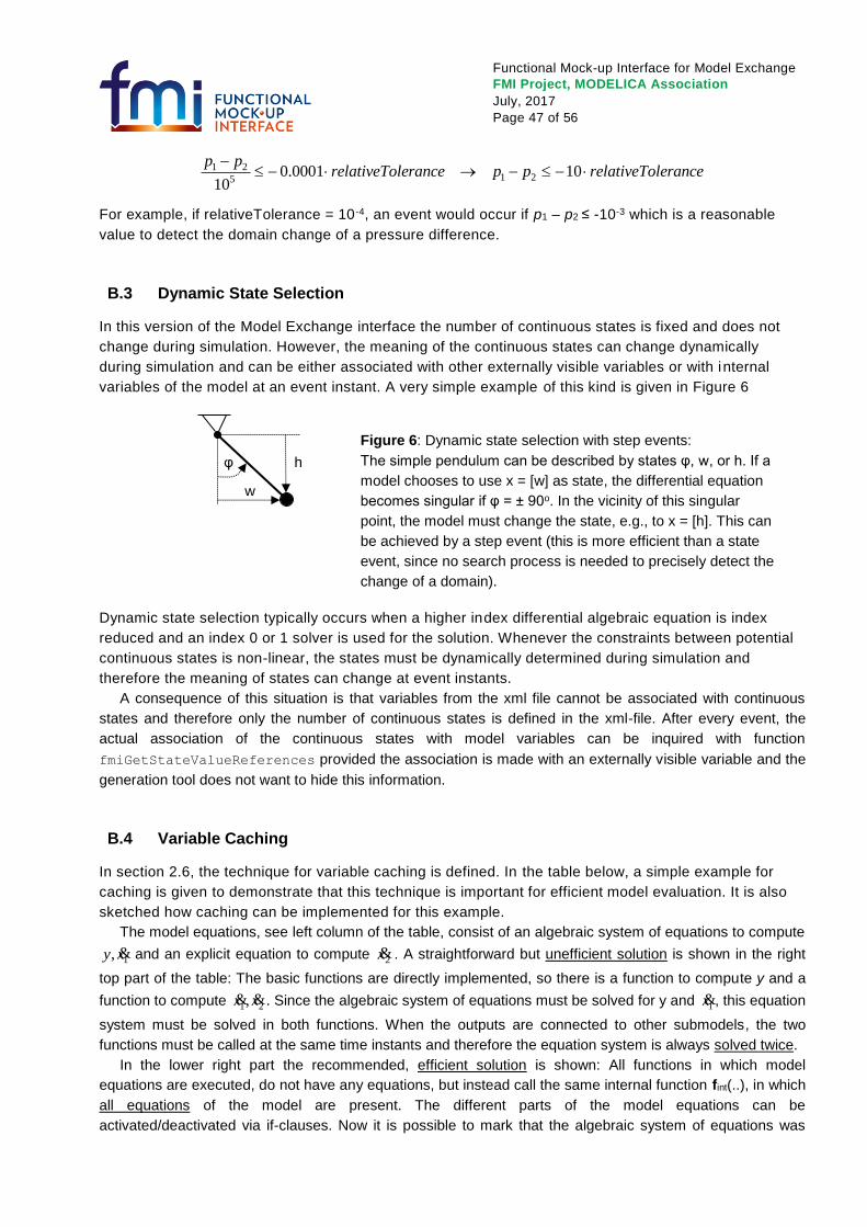
Functional Mock-up Interface for Model Exchange
FMI Project, MODELICA Association
July, 2017
Page 47 of 56
1 21 25
0.0001 1010
p prelativeTolerance p p relativeTolerance
For example, if relativeTolerance = 10 -4, an event would occur if p1 – p2 ≤ -10-3 which is a reasonable
value to detect the domain change of a pressure difference.
B.3 Dynamic State Selection
In this version of the Model Exchange interface the number of continuous states is fixed and does not
change during simulation. However, the meaning of the continuous states can change dynamically
during simulation and can be either associated with other externally visible variables or with internal
variables of the model at an event instant. A very simple example of this kind is given in Figure 6
Dynamic state selection typically occurs when a higher index differential algebraic equation is index
reduced and an index 0 or 1 solver is used for the solution. Whenever the constraints between potential
continuous states is non-linear, the states must be dynamically determined during simulation and
therefore the meaning of states can change at event instants.
A consequence of this situation is that variables from the xml file cannot be associated with continuous
states and therefore only the number of continuous states is defined in the xml-file. After every event, the
actual association of the continuous states with model variables can be inquired with function
fmiGetStateValueReferences provided the association is made with an externally visible variable and the
generation tool does not want to hide this information.
B.4 Variable Caching
In section 2.6, the technique for variable caching is defined. In the table below, a simple example for
caching is given to demonstrate that this technique is important for efficient model evaluation. It is also
sketched how caching can be implemented for this example.
The model equations, see left column of the table, consist of an algebraic system of equations to compute
1,y x& and an explicit equation to compute 2x& . A straightforward but unefficient solution is shown in the right
top part of the table: The basic functions are directly implemented, so there is a function to compute y and a
function to compute 1 2,x x& &. Since the algebraic system of equations must be solved for y and 1x&, this equation
system must be solved in both functions. When the outputs are connected to other submodels, the two
functions must be called at the same time instants and therefore the equation system is always solved twice.
In the lower right part the recommended, efficient solution is shown: All functions in which model
equations are executed, do not have any equations, but instead call the same internal function fint(..), in which
all equations of the model are present. The different parts of the model equations can be
activated/deactivated via if-clauses. Now it is possible to mark that the algebraic system of equations was
w
h φ
Figure 6: Dynamic state selection with step events:
The simple pendulum can be described by states φ, w, or h. If a
model chooses to use x = [w] as state, the differential equation
becomes singular if φ = ± 90o. In the vicinity of this singular
point, the model must change the state, e.g., to x = [h]. This can
be achieved by a step event (this is more efficient than a state
event, since no search process is needed to precisely detect the
change of a domain).
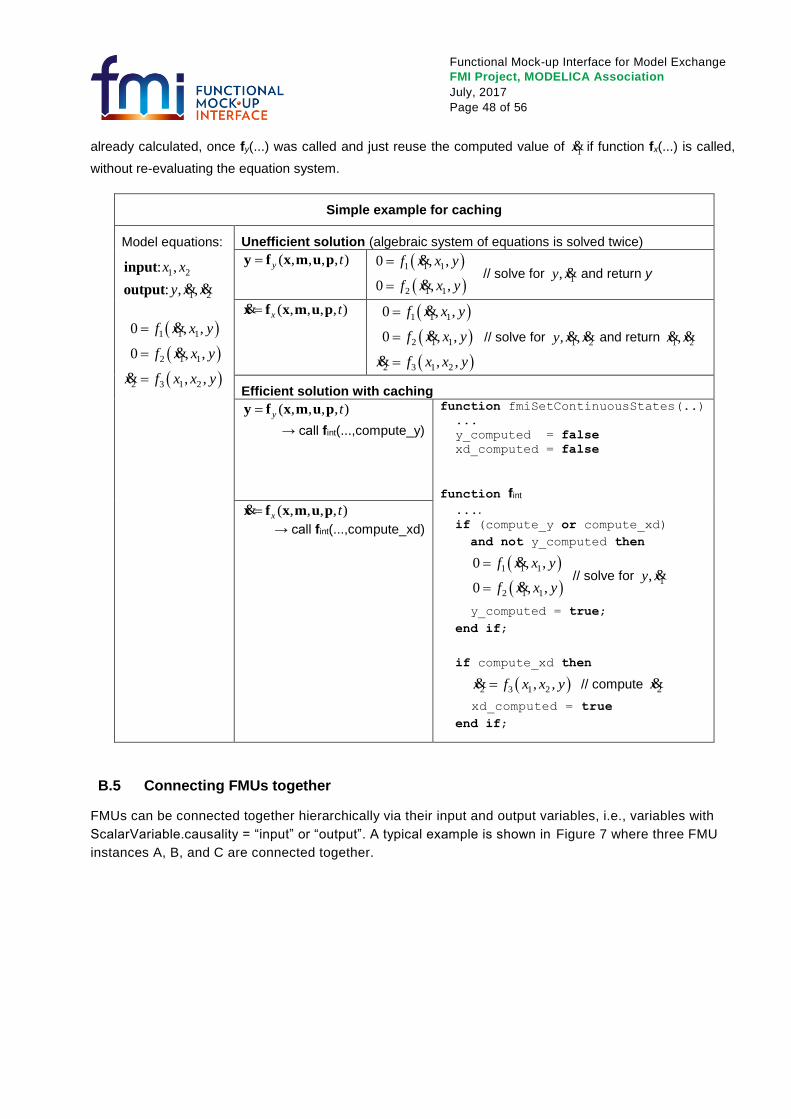
Functional Mock-up Interface for Model Exchange
FMI Project, MODELICA Association
July, 2017
Page 48 of 56
already calculated, once fy(...) was called and just reuse the computed value of 1x& if function fx(...) is called,
without re-evaluating the equation system.
B.5 Connecting FMUs together
FMUs can be connected together hierarchically via their input and output variables, i.e., variables with
ScalarVariable.causality = “input” or “output”. A typical example is shown in Figure 7 where three FMU
instances A, B, and C are connected together.
Simple example for caching
Model equations:
1 2
1 2
: ,
: , ,
x x
y x x
input
output & &
1 1 1
2 1 1
2 3 1 2
0 , ,
0 , ,
, ,
f x x y
f x x y
x f x x y
&
&
&
Unefficient solution (algebraic system of equations is solved twice)
( , , , , )y ty f x m u p
1 1 1
2 1 1
0 , ,
0 , ,
f x x y
f x x y
&
& // solve for 1,y x& and return y
( , , , , )x tx f x m u p&
1 1 1
2 1 1
2 3 1 2
0 , ,
0 , ,
, ,
f x x y
f x x y
x f x x y
&
&
&
// solve for 1 2, ,y x x& & and return 1 2,x x& &
Efficient solution with caching
( , , , , )y ty f x m u p
→ call fint(...,compute_y)
function fmiSetContinuousStates(..)
...
y_computed = false
xd_computed = false
function fint
.... if (compute_y or compute_xd)
and not y_computed then
1 1 1
2 1 1
0 , ,
0 , ,
f x x y
f x x y
&
& // solve for 1,y x&
y_computed = true;
end if;
if compute_xd then
2 3 1 2, ,x f x x y& // compute 2x&
xd_computed = true
end if;
( , , , , )x tx f x m u p&
→ call fint(...,compute_xd)
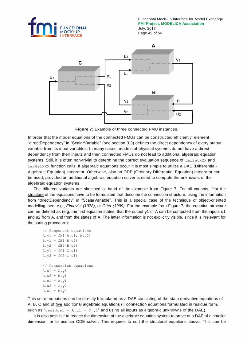
Functional Mock-up Interface for Model Exchange
FMI Project, MODELICA Association
July, 2017
Page 49 of 56
Figure 7: Example of three connected FMU instances.
In order that the model equations of the connected FMUs can be constructed efficiently, element
“directDependency” in “ScalarVariable” (see section 3.3) defines the direct dependency of every output
variable from its input variables. In many cases, models of physical systems do not have a direct
dependency from their inputs and then connected FMUs do not lead to additional algebraic equation
systems. Still, it is often non-trivial to determine the correct evaluation sequence of fmiSetXXX and
fmiGetXXX function calls. If algebraic equations occur it is most simple to utilize a DAE (Differential-
Algebraic-Equation) integrator. Otherwise, also an ODE (Ordinary-Differential-Equation) integrator can
be used, provided an additional algebraic equation solver is used to compute the unknowns of the
algebraic equation systems.
The different variants are sketched at hand of the example from Figure 7. For all variants, first the
structure of the equations have to be formulated that describe the connection structure, using the information
from “directDependency” in “ScalarVariable”. This is a special case of the technique of object-oriented
modelling, see, e.g., Elmqvist (1978), or Otter (1999). For the example from Figure 7, the equation structure
can be defined as (e.g. the first equation states, that the output y1 of A can be computed from the inputs u1
and u2 from A, and from the states of A. The latter information is not explicitly visible, since it is irrelevant for
the sorting procedure):
// Component equations
A.y1 = fA1(A.u1, A.u2)
B.y1 = fB1(B.u2)
B.y2 = fB2(B.u2)
C.y1 = fC1(C.u1)
C.y2 = fC2(C.u1)
// Connection equations
A.u1 = C.y1
A.u2 = B.y1
B.u1 = A.y1
B.u2 = C.y2
C.u1 = B.y2
This set of equations can be directly formulated as a DAE consisting of the state derivative equations of
A, B, C and of five additional algebraic equations (= connection equations formulated in residue form,
such as “residue1 = A.u1 – C.y1” and using all inputs as algebraic unknowns of the DAE).
It is also possible to reduce the dimension of the algebraic equation system to arrive at a DAE of a smaller
dimension, or to use an ODE solver. This requires to sort the structural equations above. This can be
A
B
C y1
y1
y1
y2
y2
u2
u1
u1
u1
u2
Functional Mock-up Interface for Model Exchange
FMI Project, MODELICA Association
July, 2017
Page 50 of 56
performed with the algorithms as used in object-oriented modelling. Especially, “BLT” (Block-Lower-
Triangular) transformation can be used to sort the equations and “Tearing” can be used to reduce the
dimensions of the remaining algebraic equation systems. The details of these algorithms can be found, e.g.,
in Elmqvist (1978), section 5.2, or Otter (1999). A third alternative is to not support algebraic equations of
connected FMUs and use a pure ODE solver. In the latter case it is sufficient to use the “strongConnect”
algorithm of Tarjan6, see Tarjan (1972) or Elmqvist (1978). Using BLT on the example above results in:
// Algebraic system of equations (unknowns: B.u2, C.u1)
B.y2 := fB2(B.u2)
C.y2 := fC2(C.u1)
residue1 = B.u2 - C.y2
residue2 = C.u1 - B_y2
// Sequence of equations
B.u2 := C.y2
B.y1 := fB1(B.u2)
C.y1 := fC1(C.u1)
A.u1 := C.y1
A.u2 := B.y1
A.y1 := fA1(A.u1, A.u2);
The size of the algebraic system can be further reduced by tearing leading to:
// Teared algebraic system of equations (unknowns: B.u2)
B.y2 := fB2(B.u2)
C.u1 := B.y2
C.y2 := fC2(C.u1)
residue1 = B.u2 – C.y2
As a result, this example can be formulated as a DAE consisting of the state derivative equations of A,
B, C and of one additional algebraic equation. Alternatively, an ODE integrator can be used to solve the
equations. This requires to solve an algebraic equation system with a non-linear algebraic equation
solver whenever the derivatives have to be computed. The latter approach can be implemented in the
following way (the integrator provides all states and the model has to compute the state derivatives):
// Set actual time instant
fmiSetTime( < of A > );
fmiSetTime( < of B > );
fmiSetTime( < of C > );
// Set continuous states of all components (provided by integrator)
fmiSetContinuousStates( < of A > );
fmiSetContinuousStates( < of B > );
fmiSetContinuousStates( < of C > );
// Solve algebraic system of equations
// input: B.u2, output: residue1
< start of non-linear algebraic solver >
fmiSetReal( < B.u2 > )
fmiGetReal( < B.y2 > )
fmiSetReal( < C.u1 = B.y2 > )
fmiGetReal( < C.y2 > )
6 Since only input/output blocks are here connected together, the first part of BLT to find an assignment for every variable is
trivial: All left hand side variables of the component and connection equations are the assigned variables. Then, a directed
graph is constructed with all input and output variables as nodes and the structural dependencies as edges. With function
strongConnect(..) of Tarjan (1972), it can be detected that no loops are present and the evaluation sequence is determined.
Functional Mock-up Interface for Model Exchange
FMI Project, MODELICA Association
July, 2017
Page 51 of 56
residue1 = B.u2 – C.y2
< end of non-linear algebraic solver >
// Compute the remaining inputs and outputs of all components
fmiGetReal( < B.y1 > )
fmiGetReal( < C.y1 > )
fmiSetReal( < A.u1 = C.y1 > )
fmiSetReal( < A.u2 = B.y1 > )
fmiGetReal( < A.y1 > )
// Compute the state derivatives of all components (provide to integrator)
fmiGetDerivatives( < of A > )
fmiGetDerivatives( < of B > )
fmiGetDerivatives( < of C > )
It is of course also possible to connect FMUs together with acausal components and not only to
input/output blocks. The above scheme does not change in this case. An important application is to
import an FMU in to a Modelica model, see Modelica (2009). Since a Modelica simulation environment
has all necessary algorithms for connecting acausal and causal components together, the FMUs must
only be appropriately interfaced. One simple way is to generate a Modelica wrapper model using the
information available in the xml-file of the corresponding FMU (note, this technique can be generally
applied for most simulation environments).
Functional Mock-up Interface for Model Exchange
FMI Project, MODELICA Association
July, 2017
Page 52 of 56
Appendix C Features for Future Versions
In this appendix, features are summarized that are already known to be missing and might be added in a
future release.
Improved initialization
The fmiInitialize function can currently only be called once for one instance. It might be necessary
to improve this, in order to better handle algebraic loops between connected FMUs. Note, even if
fmiInitialize can only be called once, an event can be triggered and then event iteration via
fmiEventUpdate is possible at the initial time.
Better handling of time events
Time events should be defined with an absolute precision. This requires to introduce “time” as integer
variable. The (absolute) time resolution for a simulation model is specified globally. Time can only
advance in steps of the time resolution. A submodel may have a different (absolute) time resolution (e.g.
a controller running on a particular micro-processor). Furtherore, improved support for periodically
sampled systems is needed to enhance efficiency.
Dense and sparse Jacobian
An analytic or approximate analytic Jacobian might be directly computed with a new function. Dense and
sparse Jacobians must be supported. Optionally, also only the structure of the Jacobian might be reported
(and the simulation environment computes the Jacobian numerically, but taking into account the zero/non-
zero pattern).
Saving and restoring a model state
It should be possible to stop a simulation, safe the model state and restart the simulation exactly at the
place where the simulation was stopped. The interface could be defined in the following way:
Additions to fmiModelTypes.h:
typedef char fmiByte; // byte data type
Additions to fmiModelFunctions.h:
fmiStatus = fmiGetModelStateDimension(fmiComponent c, size_t *nModelState);
fmiStatus = fmiGetModelState(fmiComponent c, fmiByte modelState[], size_t nModelState);
fmiGetModelState returns the complete state of model "c", in order that the complete internal data
structure of "c" can be reconstructed. "modelState" is a byte vector of length "nModelState". This
vector must be allocated by the calling environment before fmiGetModelState is called. In order that
this is possible fmiGetModelStateDimension returns the needed length of the vector.
fmiStatus = fmiSetModelState(fmiComponent c, fmiByte modelState[], nModelState);
The current model "c" is replaced by a previous state defined by byte vector "modelState".
"modelState" must be the vector returned by a previous call to fmiGetModelState of exactly the same
model. After calling fmiSetModelState, the model is in state "stepAccepted".
There are open issues: fmiGetModelState should only be callable directly after an event (it might be a
step event), in order that restarting the integration is a standard operation (restart after an event). Otherwise,
Functional Mock-up Interface for Model Exchange
FMI Project, MODELICA Association
July, 2017
Page 53 of 56
the integrator might be in an inconsistent state. Most likely restrictions are needed, in order that restarting a
model is possible, e.g., restarting is not possible, if a model accesses external resources, like files or
communication channels. In the xml-file it could be defined, whether it is allowed to “safe the model state” or
whether this is not possible.
Changing dimension of state vector and of event indicator vector
Submodels in a system might be enabled or disabled. To handle this efficiently, the states of the
disabled components should not be integrated. This could be achieved by defining a maximum
dimension of the state vector “nx_max” and of the event indicators “nz_max” in the Model Description
File. An actual dimension (nx,nz) is determined during initialization and at events (nx <= nx_max, nz <=
nz_max). Since the Model Exchange functions copy the return values from its internal data structure to
the interface, it is not much burden to change this copy operation ones less or more values must be
copied. Therefore, two additional return arguments (nx, nz) might be provided for initialization and for
eventUpdate.
Special handling of multi-body systems
SIMPACK has the feature that the generated code may contain both the model with integrators (using
the specialized handling of large multi-body systems) and the model without integrators. The benefit is
that the user can easily switch between both representation forms according to his needs.
Furthermore, multi-body programs are usually DAEs with a very special structure and this structure
might be revealed in the interface to allow an efficient solution.
Online changeable parameters for real-time training simulators
Parameters are constant although, it would be useful to change them online, e.g., fo r real-time training
simulators, or for quickly tuning parameters in offline simulation. From a mathematical point of view,
changing a parameter has to be seen as a short-hand notation to stop the simulation and initialize a new
simulation run with the previous internal model state where the desired parameters are changed.
Map variable hierarchy to xml file
The current Model Description File can only handle scalar variables. This means that a lot of definitions
must be repeated if, e.g., an array is mapped to a set of scalars. The xml file should be enhanced, so
that, e.g., array and record structures are maintained. A handle of a variable might be computed from a
new function, that gets the handle of the array and the desired indices. The benefit is that the xml -file
becomes much smaller if large variable arrays are present.
DAE representation
Models could be optionally described by DAEs with index 1 or 2. The benefit is that larger systems can
be handled because systems of equations are only solved once and not twice (with an ODE description,
equation systems might be solved inside the ODE description, and a stiff solver will additionally solve
equation systems in the integrator), and the sparsity of the Jacobian might be larger.
Nested FMUs with several model zip-files
In the current version, nested FMUs are stored in one zip-file and the hierarchical FMU structuring is not
exposed. This should be improved, e.g., so that every FMU is distributed in its own model zip -file which
is referenced in other FMUs.

Functional Mock-up Interface for Model Exchange
FMI Project, MODELICA Association
July, 2017
Page 54 of 56
Support for Optimization
In order to improve optimization (parameter as well as trajectory optimization), it is useful to get more
information from a model, instead of constructing this information from the available interfaces via purely
numerical methods. For example, it would be useful to provide a function to get the partial derivatives of
the state derivatives with respect to selected parameters.
Functional Mock-up Interface for Model Exchange
FMI Project, MODELICA Association
July, 2017
Page 55 of 56
Appendix D Glossary
This glossary is a subset of (MODELISAR Glossary, 2009) with some extensions specific to this
document.
Term Description
AUTOSAR AUTomotive Open System Architecture (www.autosar.org).
Evolving standard of the automotive industry to define the implementation of
embedded systems in vehicles including communication mechanisms. An
important part is the standardization of C-functions and macros to communicate
between software components. AUTOSAR is targeted to built on top of the real-
time operating system OSEK (www.osek-vdx.org, de.wikipedia.org/wiki/OSEK).
The use of the AUTOSAR standard requires AUTOSAR membership.
co-simulation Couple several simulation programs including their numerical solvers in order to
simulate a system consisting of several subsystems.
ECU Electronic Control Unit (Microprocessor that is used to control a sub-system in a
vehicle)
event The time instant at which the integration is halted and variables may change their
values discontinuously. Between event instants, all variables are continuous.
FMI Functional Mock-up Interface:
Interface of a functional mock-up in form of a model. In analogy to the term digital
mock-up (see mock-up), functional mock-up describes a computer-based
representation of the functional behaviour of a system for all kinds of analyses.
FMU Functional Mock-up Unit:
A “model class” from which one or more “model instances” can be build for
simulation. A FMU is stored in one zip-file as defined in section 4 consisting
basically of one xml file (see section 3) that defines the model variables and a set
of C-functions (see section 2), in source or binary form, to execute the model
equations.
mock-up A full-sized structural, but not necessarily functional model built accurately to
scale, used chiefly for study, testing, or display. In the context of computer aided
design (CAD), a digital mock-up (DMU) means a computer-based representation
of the product geometry with its parts, usually in 3-D, for all kinds of geometrical
and mechanical analyses.
model A model is a mathematical or logical representation of a system of entities,
phenomena, or processes. Basically a model is a simplified abstract view of the
complex reality. It can be used to compute its expected behaviour under
specified conditions. In this document, “models” are described by differential,
algebraic and discrete equations and are mainly used to represent physical
systems and controllers.
Model Description
Schema
An XML schema that defines how all relevant, non-executable, information about
a “model class” (FMU) is stored in a text file in XML format. Most important, data
for every variable is defined (variable name, handle, data type, variability, unit,
etc.), see section 3.
Model Interface A set of C-interface definitions to access the equations of a dynamic system from
an external program, e.g., to compute the state derivatives of a model, see
section 2.
Functional Mock-up Interface for Model Exchange
FMI Project, MODELICA Association
July, 2017
Page 56 of 56
Term Description
parameter A quantity within a model, which remains constant during simulation, but may be
changed before a simulation is started. Examples: mass, stiffness, resistance,
etc.
state The “continuous states” of a model are all variables that appear differentiated in
the model and are independent from each other.
The “discrete states” of a model are time-discrete variables that have two values
in a model: The value of the variable from the previous event instant, and the
value of the variable at the actual event instant.
state event Event that is defined by the time instant where the domain z > 0 of an event
indicator variable z is changed to z ≤ 0, or vice versa.
This definition is slightly different as the usual standard definition of state events:
“z(t)*z(ti-1) ≤ 0” which has the severe drawback that the value of the event
indicator at the previous event instant, z(ti-1) ≠ 0, must be non-zero and this
condition cannot be guaranteed. The often used term “zero crossing function” for
z is misleading (and is therefore not used in this document), since a state event is
defined by a change of a domain and not by a zero crossing of a variable.
step event Event that might occur at a completed integrator step. Since this event type is not
defined by a precise time or condition, it is usually not defined by a user. A
program may use it, e.g., to dynamically switch between different states (see
Figure 6 in Appendix B.3). A step event is handled much more efficiently than a
state event, because the event is just triggered after performing a check at a
completed integrator step, whereas a search procedure is needed for a state
event.
time event Event that is defined by a predefined time instant. Since the time instant is known
in advance, the integrator can select its step size so that the event point is
directly reached. Therefore, this event can be handled efficiently.
XML eXtensible Markup Language (www.w3.org/XML, en.wikipedia.org/wiki/Xml) – An
open standard to store information on text files in a structured form.


![Efficient Model Transformation Languagesmsdl.cs.mcgill.ca/.../2016/Lara_Antonio_cosimulation.pdf · 2018-01-04 · Solution: Functional Mock-up Interface Standard [2] •Simulator](https://img.pdfslide.net/doc/110x75/5f854c16d375f63fc67e93a0/efficient-model-transformation-2018-01-04-solution-functional-mock-up-interface.jpg)