Functions, commodities and environmental impacts in an ecological–economic model

www.elsevier.com/locate/ecolecon

Ecological Economics 48 (2004) 451–467

ANALYSIS

Functions, commodities and environmental impacts in an

ecological–economic model

Sangwon Suh*

Institute of Environmental Sciences (CML), Leiden University, P.O. Box 9518, NL-2300RA Leiden, The Netherlands

Received 12 May 2003; received in revised form 20 October 2003; accepted 23 October 2003

Abstract

In contrast to macroscopic tools, life cycle assessment (LCA) starts from the microstructure of an economic system: the

production and consumption of functional flows. Due to the level of resolution required for function-level details, the model

used for LCA has relied on process-specific data and has treated the product system as a stand-alone system instead of a system

embedded within a broader economic system. This separation causes various problems, including incompleteness of the system

and loss of applicability for a variety of analytical tools developed for LCA or economic models. This study aims to link the

functional flow-based, micro-level LCA system to its embedding, commodity-based, meso- or macro-level economic system

represented by input–output accounts, resulting in a comprehensive ecological–economic model within a consistent and

flexible mathematical framework. For this purpose, the LCA computational structure is reformulated into a functional flow by

process framework and reintroduced in the context of the input–output tradition. It is argued that the model presented here

overcomes the problem of incompleteness of the system and enables various analytical tools developed for LCA or input–

output analysis (IOA) to be utilised for further analysis. The applicability of the model for cleaner production and supply chain

management is demonstrated using a simplified product system and structural path analysis as an example.

D 2004 Elsevier B.V. All rights reserved.

Keywords: Life cycle assessment (LCA); Input–output analysis (IOA); Hybrid analysis; System boundary; Comprehensive ecological–

economic model; Functional flow

1. Introduction

Since the beginning of the last century, ecologists

have been borrowing ideas and concepts from econom-

ics. Entities in an ecosystem are viewed as economic

agents that process materials and energy, terms like

producers and consumers have been widely adopted in

ecology, and productivity and efficiency have become

the main interests of ecologists (Worster, 1994).

0921-8009/$ - see front matter D 2004 Elsevier B.V. All rights reserved.

doi:10.1016/j.ecolecon.2003.10.013

* Tel.: +31-71-527-7460; fax: +31-71-527-7434.

E-mail address: [email protected] (S. Suh).

Recently, there has been a movement in the oppo-

site direction as well, in that principles of ecology

have come to be utilised for industrial and economic

systems. In the field of industrial ecology, for in-

stance, an industrial system is viewed as a self-

organising system, with interest focusing on its me-

tabolism, which describes how materials and energy

are processed, used and disposed of (see e.g. Ayres

and Ayres, 1996; Graedel and Allenby, 1995). One

pillar of the industrial metabolism discourse is the role

of commodities. An obvious role of commodities and

their supply network is the circulation of materials and

S. Suh / Ecological Economics 48 (2004) 451–467452

energy in an economy, which, in turn, generates

pollutants and wastes and causes environmental

impacts. The circulation of materials and energy and

the generation of pollutants and wastes characterise

the physical terms of commodities in an economic

system, while what is more interesting from the

economics side is the utilities or functions of com-

modities, which actually lead consumers to demand

the commodity (Sen, 1999). Thus, it is not only the

physical implications but also the functions of com-

modities that are essential in describing the metabolic

structure of an economic system.

The present paper concerns the connection be-

tween the physical and the functional terms of

commodities in a model which is called here eco-

logical–economic, and which describes materials

and energy exchanges within and between the eco-

nomic system and the environment. The model is

structured on the basis of an extended framework of

life cycle assessment (LCA).

LCA describes the microstructure of an ecologi-

cal–economic system, its main focus being the

production and consumption of a functional flow

and its environmental consequences (Guinee et al.,

2002). This bottom-up approach concerns prevention

of pollution at the level of production and consump-

tion of a specific product, or more precisely, a

specific function of a product, through eco-labelling,

process redesign, cleaner production, supply chain

management, etc. Thus, the model needed by LCA

should, on the one hand, be able to describe indi-

vidual processes and their interrelations in detail

and, on the other hand, be system-encompassing.

In practice, however, the two objectives, i.e. level of

detail and system completeness, are difficult to attain

at the same time. As the number of inputs increases

through upstream processes, system analysts have to

stop compiling upstream data at a certain stage, or

they have to use more aggregated data, thus losing

process specificity. Most LCA studies opt for pro-

cess specificity, rather than for completeness of the

system.

Attempts to overcome the incompleteness of a

process analysis by using input–output analysis

(IOA) are generally referred to as hybrid analysis

(see e.g. Bullard et al., 1978). However, the model

structures of process analysis and IOA have not been

fully integrated in hybrid analyses so far. Hybrid

analysis, including hybrid energy analysis, utilises

matrix representation only for the input–output part,

while process analysis is dealt with separately by

using a process flow diagram approach. This separa-

tion in the computational structure imposes several

constraints on hybrid models.

The main questions addressed by the present paper

are ‘how can we better link the microstructure of an

ecological–economic system dealt with in LCA to its

embedding economic system?’, and ‘what are the

relevant forms and structures of the LCA and IOA

that are to be integrated?’. To answer these questions,

I present a model that integrates the computational

structures of IOA and LCAwithin a consistent frame-

work, enabling various analytical tools to be applied

to the model.

2. Survey of hybrid models

The general framework of hybrid analysis was

introduced as early as the 1970s in the context of

energy analysis. The discipline of energy analysis has

used process analysis—or vertical analysis—and in-

put–output based energy analysis in parallel for slight-

ly different purposes (see IFIAS, 1974). It was Bullard

and Pillati (1976); Bullard et al. (1978) who calculated

the net energy requirements of a product by combining

the results of process analysis and IOA. This allowed

the incomplete system of process-based energy analy-

ses to be significantly improved. In the field of input–

output energy analysis, the approach developed by

Bullard and his colleagues has become common prac-

tice, and many empirical studies are available (see e.g.

Engelenburg et al., 1994; Wilting, 1996).

Input–output techniques have been studied as a

tool for LCA since the early 1990s. Moriguchi et al.

(1993) were the first to analyse the life-cycle CO2

emissions of an automobile, using both the Japanese

input–output table and process analysis. Since the

study by Moriguchi et al. (1993), there have been

many LCA studies and software tools using input–

output techniques, including Lave et al. (1995); Tre-

loar (1997); Marheineke et al. (1998); Hendrickson et

al. (1998); Joshi (2000); Suh and Huppes (2002) (see

Suh et al., (2004) for detail).

Although the area of application, the level of

aggregation and the number of pollutants covered

S. Suh / Ecological Economics 48 (2004) 451–467 453

in these studies vary, the result of a hybrid analysis

has been the simple sum of process analysis and

input–output based analysis. In other words, the

computational structure of LCA has not been fully

integrated with that of IOA, which creates several

difficulties.

One problem is that the commodity flows de-

scribed in the process-based system are, in principle,

also described in the input–output system, which

leads to misspecification through double counting.1

Furthermore, current hybrid techniques are unable

to systematically model the interactive relationship

between process-based system and input–output

system through both inputs and outputs. For exam-

ple, in analysing different options of reusing or

recycling wastes from the disposal phase of a

product system, each option simultaneously changes

the input structure not only of the process-based

system but also of the input–output based system. It

is important to note that the relationship between the

process-based system and the input–output based

system, representing the microstructure of the com-

modity flows web and the wider, embedding econ-

omy, respectively, is interactive, and that an

integrated model is required to represent this inter-

active relation.

In addition, there are also practical difficulties in

using analytical tools consistently. Various analytical

tools have been developed for LCA or IOA, including

structural decomposition analysis, structural path

analysis, field of influence analysis, Monte Carlo

simulation, perturbation analysis, linear programming,

sensitivity analysis etc. In implementing the compu-

tations for these analyses, each system has to be

treated differently, due to the difference in computa-

tional structure, resulting in loss of consistency.

1 Suppose a simplified case that an industry sector in an input–

output table, for instance, automobile manufacturing includes

passenger cars and trucks, which shares 80% and 20% of the total

sales, respectively. A process-based LCA study compiled process-

specific data for production of passenger cars within the process-

based system. There are, however, some missing inputs of trucks,

and they are to be linked to a relevant input–output sector, which is,

in this case, the automobile manufacturing, through a hybrid model.

However, the sector in an input–output based system still includes

the passenger car manufacturing processes, so that those inputs are

misspecified as 80% of passenger cars and only 20% trucks.

3. Computational structures of IOA and LCA

3.1. Input–output analysis (IOA)

The basic computational structure of input–output

models is briefly discussed here, based on Leontief

(1936); Leontief (1941). Leontief’s model starts with

transaction records between industries within a na-

tional economy.2 Let us define the transaction matrix

Z such that (Z)ij indicates the amount of domestic

industry output purchased by industry j from domestic

industry i in monetary terms. By assuming that each

industry produces only one distinct output, we obtain

a square transaction matrix Z. It is a convention in

input–output economics that the transaction matrix is

converted into a coefficient matrix, which is generally

called the direct requirement matrix. Let g be the total

industry output vector such that (g)i shows the amount

of the total output by industry i, which is the sum of

the total output of the industry that is consumed by

domestic industries, households and export. An in-

dustry-by-industry direct requirements matrix, A, is

then defined by

A ¼ Zg�1: ð1Þ

The hat (ˆ) in (1) makes a diagonal matrix out of a

vector, such that (g)i is located at (g)ii and (g)ij = 0,

where i p j. An element of the direct requirements

matrix (A)ij shows the amount of industry output i

required by industry j to produce a unit of its output.

An equality

g � Ag ¼ f ð2Þ

holds in a national economy where the total amount of

domestic industry output produced (g) minus the total

industry output consumed by domestic industries (Ag)

equals the amount of industry output consumed by

final consumers and export (f) (Leontief, 1941).

Rearranging (2) gives

g ¼ ðI� AÞ�1f ð3Þ

for non-singular (I�A). Assuming further that the

input structure of each industry does not change when

2 Imports and capital investment have been omitted here for the

sake of simplicity, but are dealt with in a later section.

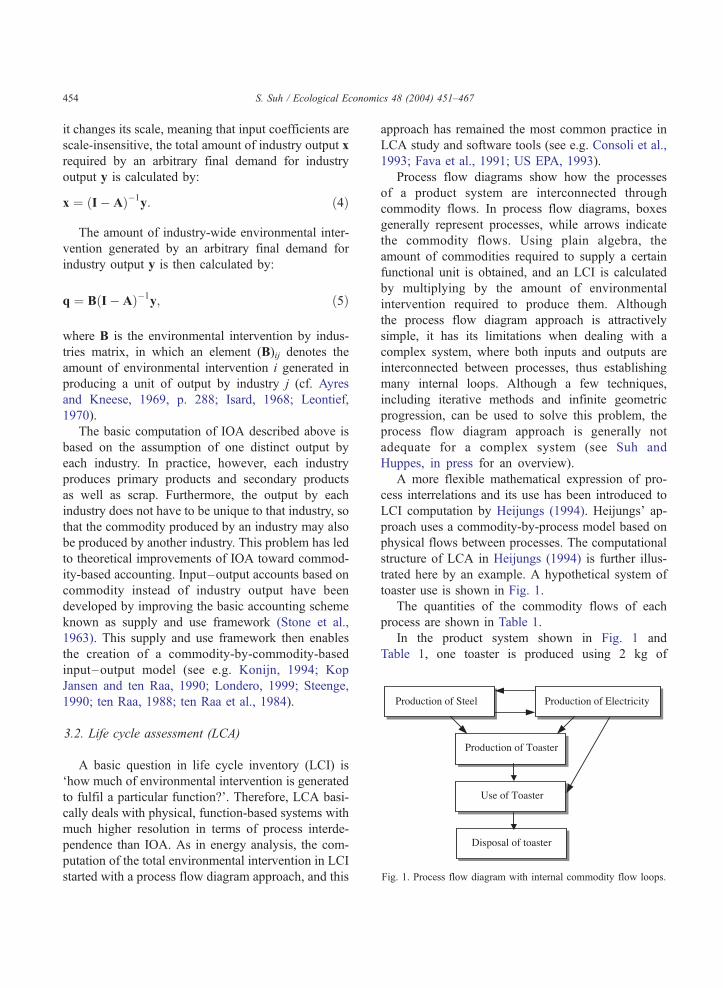
Fig. 1. Process flow diagram with internal commodity flow loops.


it changes its scale, meaning that input coefficients are

scale-insensitive, the total amount of industry output x

required by an arbitrary final demand for industry

output y is calculated by:

x ¼ ðI� AÞ�1y: ð4Þ

The amount of industry-wide environmental inter-

vention generated by an arbitrary final demand for

industry output y is then calculated by:

q ¼ BðI� AÞ�1y; ð5Þ

where B is the environmental intervention by indus-

tries matrix, in which an element (B)ij denotes the

amount of environmental intervention i generated in

producing a unit of output by industry j (cf. Ayres

and Kneese, 1969, p. 288; Isard, 1968; Leontief,

1970).

The basic computation of IOA described above is

based on the assumption of one distinct output by

each industry. In practice, however, each industry

produces primary products and secondary products

as well as scrap. Furthermore, the output by each

industry does not have to be unique to that industry, so

that the commodity produced by an industry may also

be produced by another industry. This problem has led

to theoretical improvements of IOA toward commod-

ity-based accounting. Input–output accounts based on

commodity instead of industry output have been

developed by improving the basic accounting scheme

known as supply and use framework (Stone et al.,

1963). This supply and use framework then enables

the creation of a commodity-by-commodity-based

input–output model (see e.g. Konijn, 1994; Kop

Jansen and ten Raa, 1990; Londero, 1999; Steenge,

1990; ten Raa, 1988; ten Raa et al., 1984).

3.2. Life cycle assessment (LCA)

A basic question in life cycle inventory (LCI) is

‘how much of environmental intervention is generated

to fulfil a particular function?’. Therefore, LCA basi-

cally deals with physical, function-based systems with

much higher resolution in terms of process interde-

pendence than IOA. As in energy analysis, the com-

putation of the total environmental intervention in LCI

started with a process flow diagram approach, and this

approach has remained the most common practice in

LCA study and software tools (see e.g. Consoli et al.,

1993; Fava et al., 1991; US EPA, 1993).

Process flow diagrams show how the processes

of a product system are interconnected through

commodity flows. In process flow diagrams, boxes

generally represent processes, while arrows indicate

the commodity flows. Using plain algebra, the

amount of commodities required to supply a certain

functional unit is obtained, and an LCI is calculated

by multiplying by the amount of environmental

intervention required to produce them. Although

the process flow diagram approach is attractively

simple, it has its limitations when dealing with a

complex system, where both inputs and outputs are

interconnected between processes, thus establishing

many internal loops. Although a few techniques,

including iterative methods and infinite geometric

progression, can be used to solve this problem, the

process flow diagram approach is generally not

adequate for a complex system (see Suh and

Huppes, in press for an overview).

A more flexible mathematical expression of pro-

cess interrelations and its use has been introduced to

LCI computation by Heijungs (1994). Heijungs’ ap-

proach uses a commodity-by-process model based on

physical flows between processes. The computational

structure of LCA in Heijungs (1994) is further illus-

trated here by an example. A hypothetical system of

toaster use is shown in Fig. 1.

The quantities of the commodity flows of each

process are shown in Table 1.

In the product system shown in Fig. 1 and

Table 1, one toaster is produced using 2 kg of

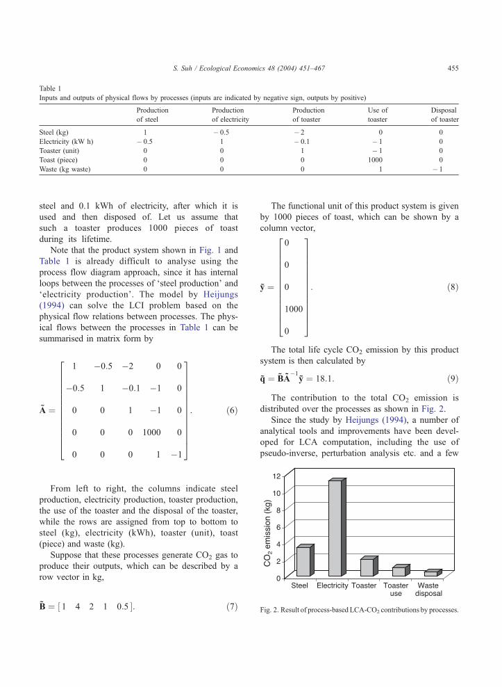
Table 1

Inputs and outputs of physical flows by processes (inputs are indicated by negative sign, outputs by positive)

Production

of steel

Production

of electricity

Production

of toaster

Use of

toaster

Disposal

of toaster

Steel (kg) 1 � 0.5 � 2 0 0

Electricity (kW h) � 0.5 1 � 0.1 � 1 0

Toaster (unit) 0 0 1 � 1 0

Toast (piece) 0 0 0 1000 0

Waste (kg waste) 0 0 0 1 � 1

Fig. 2. Result of process-based LCA-CO2 contributions by processes.


steel and 0.1 kWh of electricity, after which it is

used and then disposed of. Let us assume that

such a toaster produces 1000 pieces of toast

during its lifetime.

Note that the product system shown in Fig. 1 and

Table 1 is already difficult to analyse using the

process flow diagram approach, since it has internal

loops between the processes of ‘steel production’ and

‘electricity production’. The model by Heijungs

(1994) can solve the LCI problem based on the

physical flow relations between processes. The phys-

ical flows between the processes in Table 1 can be

summarised in matrix form by

A ¼

1 �0:5 �2 0 0

�0:5 1 �0:1 �1 0

0 0 1 �1 0

0 0 0 1000 0

0 0 0 1 �1

26666666666664

37777777777775

: ð6Þ

From left to right, the columns indicate steel

production, electricity production, toaster production,

the use of the toaster and the disposal of the toaster,

while the rows are assigned from top to bottom to

steel (kg), electricity (kWh), toaster (unit), toast

(piece) and waste (kg).

Suppose that these processes generate CO2 gas to

produce their outputs, which can be described by a

row vector in kg,

B ¼ ½ 1 4 2 1 0:5 �: ð7Þ

The functional unit of this product system is given

by 1000 pieces of toast, which can be shown by a

column vector,

y ¼

0

0

0

1000

0

26666666666664

37777777777775

: ð8Þ

The total life cycle CO2 emission by this product

system is then calculated by

q ¼ BA�1y ¼ 18:1: ð9Þ

The contribution to the total CO2 emission is

distributed over the processes as shown in Fig. 2.

Since the study by Heijungs (1994), a number of

analytical tools and improvements have been devel-

oped for LCA computation, including the use of

pseudo-inverse, perturbation analysis etc. and a few


software programs and databases have been created

using the Eq. (9) (see Heijungs and Suh, 2002).

4. IOA and LCA for integrated hybrid models

It is important to note that both environmental IOA

and LCA on their own run into serious problems as

ecological–economic models for detailed environ-

mental systems analysis. Although the input–output

model covers a wider system, including all interac-

tions between industries within a national economy,

the result is an average value of a set of processes,

while LCA also has a fundamental problem of trun-

cation. Therefore, a model is required that reveals the

microstructure of the important parts of a product

system and, at the same time, covers the entire

economic system.

As shown in the previous section, the systems

that IOA and LCA deal with have a lot in common.

Despite the similarities, however, the systems that

LCA deals with also have more than a few impor-

tant differences: there are no annual ‘transaction’

records available, quantities are in physical units, it

concerns the direction of physical flows instead of

that of money flows, it contains use and end-of-life

stages, it primarily concerns the function of a

system etc. These differences provided enough rea-

sons for LCA researchers to independently develop

slightly different computational structures from that

of IOA (see e.g. Projektgemeinschaft Lebenswegbi-

lanzen, 1991; Heijungs, 1994; Heijungs and Suh,

2002).3 Those unique features indeed make it diffi-

cult for an LCA to be directly integrated with IOA

in current form (see Section 6). The rest of this

section discusses the relevant formats and adapta-

tions required to integrate IOA and LCA, for which

I tried to reformulate the LCA model structure in

the context of input–output economics’ tradition but

only with a different set-up namely, functional flow-

by-process accounts.

The format of the input–output table used here

is the commodity-by-commodity format derived

from make and use matrices. The industry-by-in-

3 Many LCA case studies, databases and software tools

developed and used are, however, based on Heijungs (1994);

Heijungs and Suh (2002).

dustry format is less applicable in the current

model, due to the aggregation of commodities in

an industry output. Moreover, the industry that

produces an input material for a process is generally

less fully known to the LCA practitioners than the

commodity itself. In order to distinguish our format

from the industry-by-industry matrix—A in (4)—we

use AV for the commodity-by-commodity direct

requirements matrix.

Furthermore, the input–output technology coeffi-

cient matrix should include domestic and imported

capital goods, as well as domestic and imported

current products, such that

A*V ¼ ADCV þ ADKV þ AICV þ AIKV : ð10Þ

Matrices ADCV , ADKV , AICV , and AIKV , are the

commodity-by-commodity direct requirements matri-

ces for domestic current products, domestic capital

goods, imported current products and imported capital

goods, respectively, with imported current and capital

goods assigned to the relevant domestic indices. An

assumption here is that the technology and the eco-

nomic structure used to produce these imported prod-

ucts and capital goods are exactly the same as the

domestic ones (see Lenzen, 2001 for a comprehensive

treatment).

Since the available input–output table is generally

several years old, the prices should be rescaled to

current price levels as well. The input–output techni-

cal coefficient matrix A*V, in (10) is rescaled to a

coefficient matrix A**V , with current prices by

A**V ¼ pAV*p�1; ð11Þ

where vector p shows the price ratio of each com-

modity between current and the year on which the

input–output table is based. The input–output tech-

nology coefficient matrix used below refers to the

matrix with price rescaling by (11). The environmen-

tal intervention-by-industry matrix B in (5) should

also be adjusted to an environmental intervention-by-

commodity matrix, B**V , by applying an allocation

model and reflecting price differences in accordance

with the procedure outlined above.

The LCA model shown in the previous section

cannot be used directly for integration either. Here we

introduce a computational structure of LCI, based on

4 LCA case studies and databases, so far, are based on the

direction of physical flows.


the supply–demand relationship of functional flows

that will be fully integratedwith IOA in the next section.

LCA deals with the production and consumption of

functions by processes (ISO, 1998). In this context, a

function refers to a useful trait of a commodity, and a

commodity may have multiple functions (cf. Lancaster,

1966). A shampoo, for instance, may have multiple

functions, such as ‘cleaning’, ‘conditioning’, ‘moistu-

rising’, ‘protein supply’ etc. In order to refer to a

quantitative function flow, we will use the term func-

tional flow. Since a function is the basis of computation

in LCA, it means that if two shampoos are studied, they

should be compared on the basis of equivalent func-

tion(s) by subtracting or adding additional function(s).

A set of functions can also be collectively referred as a

function if individual functions need not be distin-

guished. The level of resolution used in defining a

function depends on the objective of the study. If it is

unnecessary to distinguish all functions of a commod-

ity, these functional flows can be represented by the

flow of the commodity. In this respect, commodity

flows can be good surrogates for functional flows in

many cases, though not in all.

Let us define a process as a unit activity that

produces function(s). In other words, each process

produces at least one functional flow. A process exists

because there is a demand for its functional flow from

outside the process. We shall use the demand as the

basis of the imputation of environmental intervention

and input requirements. In this context, a process may

refer to an industrial process as well as a household

activity or a post-consumer activity (cf. Sen, 1999).

A process also demands functional flows produced

by other processes for its operation. Production and

consumption of functions by a product system can be

expressed by a matrix Z*, of which a column, ðZ�Þ:jrepresents the amount of functional flows consumed

and produced over a certain period of operation by

process j being given in the relevant physical unit.

Thus, a household process like the ‘use of TV’ may

have ‘hour of TV watching’ as its functional flow

output and ‘kWh of electricity’ as an input. One clear

advantage of using physical units is that functional flow

relations between processes are not distorted by price

fluctuations over time or across consuming processes.

In compiling the vector of functional flows of a

process j, (Z*):j, the production of functional flow is

shown as a positive value, while consumption is given

a negative sign. Note here that, although these flows are

expressed in physical units, the direction of a flow may

differ from that of the physical flow.4 The direction of a

waste flow, for example, is from industrial processes to

waste treatment processes in terms of physical waste

flows, while the direction may be the opposite in terms

of functional flows, which may be ‘kg waste treatment

service’ (cf. Heijungs, 1994). Nevertheless, it is also

possible that the waste treatment facility purchases the

waste to produce other commodities such as heat or

recycled products. In this case the waste become a

functional output of the industrial process.

In most cases, except for household processes, the

direction of a functional flow between two processes is

clearly indicated by monetary transaction flows—if the

waste treatment facility purchased the waste for, e.g. its

heat content, then the waste is no longer waste, but a

functional output that has lower economic value. There

are some cases in which the direction of a functional

flow may be unclear from the monetary transaction

flow. Suppose, for example, that a waste recycling

process receives waste materials from a demolition

process for free. In this case, there is no transaction

flow between the two processes. The functional flows,

however, can be understood to have both directions: the

waste recycling process purchases the waste materials

from the demolition process, and the demolition pro-

cess purchases the waste treatment services from the

waste recycling process at exactly the same price that

they would have to pay to one another. We will refer to

the relationship between processes in producing and

consuming functional flows as a supply–demand rela-

tionship between the processes, and we will use this

relationship in imputing functional flow inputs and

environmental interventions by a process, i.e. the

demand for a functional flow by a process will get

not only the functional flow but also part of the inputs

used and environmental interventions caused by the

process in producing the functional flow.

We also make a steady-state assumption in com-

piling the vector of the functional flows of a process.

We assume that processes are operated under com-

plete steady-state conditions. In reality, of course,

hardly any industrial or consumer process is operated

under complete steady-state conditions—processes

5 It also conflicts the assumption of only one homogeneous

output per each sector, since it is not well imaginable for an industry

to buy the same product that the industry produces (see Georgescu-

Roegen, 1971; Lenzen, 2001).


may be subject to changes in production volume and

degradation in performance over time. The steady-

state condition here, however, means that we look at a

period of process operation that is long enough to

cover all the abnormalities and short enough to

represent current operating conditions, and that we

distribute all these abnormalities homogeneously over

a given period of time, resulting in an averaged typical

input–output ratio for each process. In contrast to the

input–output table, the absolute value of the time

period chosen for each process may differ between

processes. We define a vector called basis period of

steady-state approximation t, of which an element (t)ishows the size of the temporal window used for the

steady-state approximation for process i.

Let Z* be a functional flows by processes matrix

such that (Z*)ij is the amount of functional flow i used

or produced by process j during the period of time that

has been determined as the basis of steady-state ap-

proximation for process j. Note that the matrix Z* may

have more than one positive value in each column, and

may also be rectangular. A rectangular Z* should be

further treated to make it square. The rectangularity

problem is generally caused by the difference between

the row and column indices. The matrix Z*, for

instance, has functional flows as its row indices and

processes as its columns. The procedure to transform a

functional flow-by-process matrix into a functional

flow-by-production of a functional flow matrix is

referred to as allocation here (cf. Heijungs and Frisch-

knecht, 1998; Weidema, 2001). Details of the alloca-

tion procedure in this context will not be dealt with

here, but can be found elsewhere (Suh, 2001a). For the

sake of simplicity, we assume that Z* is square.

Since we have compiled Z* by assuming that each

process is operated under complete steady-state con-

ditions, the choice of a temporal window of process

operation that is smaller than the basis period of steady-

state approximation will not make any difference for

the ratio between each input and output. However, it is

convenient to define a unit operation time for each

process. The absolute value of the unit operation time

for a process may vary across processes. Avector called

unit operation time u is defined such that (u)i shows the

unit operation time chosen for process i, where

tzu: ð12Þ

For instance, the unit operation time can be chosen

in such a way that the functional flow output by each

process becomes 1 (see e.g. Heijungs, 1994). The

basis period of steady-state approximation can then be

expressed in terms of the unit operation time, such

that

t ¼ ug; ð13Þ

where g is a vector of time ratio by processes such that

(g)i shows the unit operation time, (u)i as a ratio of

basis period of steady-state approximation for process

i. Rearranging (13) gives

g ¼ u�1t: ð14Þ

We can now define the functional flow-by-process

LCA technology coefficient matrix A* by

A* ¼ Z*ð ˆgÞ�1; ð15Þ

where (A*)ij is the physical amount of functional flow

i used or produced by process j during the unit

operation time chosen. Again, a negative sign is

assigned to the use of functional flow and a positive

value to production. Note further that, unlike the

input –output technology coefficient matrix, the

LCA coefficient matrix has no values for self-con-

sumption, which is located on the main diagonal of

the intermediate part of an input–output table. The

idea of self-consumption is in fact a statistical artefact,

due to the level of aggregation in industry classifica-

tion, which is not generally the case for LCA.5 The

amount of functional flow delivered outside the sys-

tem during the basis period of steady state approxi-

mation is then calculated by

A*g ¼ f : ð16Þ

Note that an identity

f ¼ Z*i ð17Þ


holds, where i is a summation vector with only one in

a relevant dimension, and f is the total production of

functional flow. Rearranging (16) gives

g ¼ A�1

* f ð18Þ

for non-singular A*. Assuming that the coefficients of

technology coefficient matrix in (18) do not change as

the amount of functional flow delivered outside the

system changes, the amount of unit operation time x

required to produce an arbitrary final demand for

functional flow y is calculated by

x ¼ A�1

* y: ð19Þ

The total environmental intervention due to an

arbitrary final demand is then given by

q ¼ BA�1

* y; ð20Þ

where B is the environmental intervention by pro-

cess matrix, of which an element (B)ij shows the

amount of environmental intervention i generated

by process j during its unit operation time. Eq. (20)

returns the amount of environmental intervention

caused by the external demand for a particular

functional flow of a product system using the

imputation algorithm based on the supply–demand

relationship.

6 Default values for the transportation cost and wholesale

margin can be found from a use table of input–output accounts.

5. Integrated hybrid LCA

5.1. The model

In the previous section we have prepared for-

mats and computational structures for the further

integration of IOA and LCA. In this section I

present the framework of a hybrid model that fully

integrates the input–output and LCA computational

structures.

I start by defining upstream and downstream cut-

off matrices. The upstream cut-off by processes

matrix is derived by dividing the total bill of goods

for the inputs that are not covered by a processes in

a process-based system during the period of steady-

state approximation by the total unit operation time

of each process. The downstream cut-off by func-

tional flow matrix is derived by dividing the annual

sales of functional flow—in physical units that are

relevant to each functional flow—by the production

of each total commodity. In matrix notation this

becomes

Cu ¼ Zu ˆg

*�1 ð21Þ

and

Cd ¼ Zd

*ðg***Þ�1; ð22Þ

where Z*u denotes the total amount of the cut-off

commodity flows by processes during the period of

steady-state approximation in monetary terms, and

Z*d denotes the amount of annual sales of func-

tional flows from processes to input–output indus-

tries in relevant physical units (cf. Eqs. (1) and

(15)). The vector g*** shows total domestically

produced and imported current and capital goods,

with price levels updated for the difference with

the base year, and with the portion of commodity

flows represented by the process-based system

subtracted (see Appendix A). Note that the deriva-

tion of cut-off matrices has to be done in accor-

dance with the type of basic price with which the

transaction table has been compiled. If the basic

transaction table is compiled on the basis of con-

sumer’s prices, then the bill of goods for each

LCA process can be directly used to compile the

upstream cut-off matrix. If the basic price type is

the producer’s price, the information from the bill

of goods should be converted to producer’s prices

by subtracting the cost of transportation and the

wholesale margin from the amount paid.6 Skipping

this procedure can introduce considerable levels of

underestimation or overestimation in the final

results.

The resulting upstream cut-off matrix Cu is pre-

sented in such a way that (Cu)ij shows the amount of


cut-off of input–output commodity i to process j

during the unit operation time, in monetary terms.

Similarly, the downstream cut-off matrix Cd is pre-

sented in such a way that (Cd)ij shows the amount of

cut-off flows of functional flow i to input–output

commodity j per unit of monetary value of its output,

in relevant physical units.

Now we are ready to present the basic balancing

equation for integrated hybrid analysis:

A� �Cd

�Cu I� A***V

24

35

g

g ***

24

35 ¼

f

f***

24

35; ð23Þ

where A***V denotes the commodity-by-commodity

input –output technology coefficient matrix that

includes domestic and imported current products and

capital, with prices updated to current levels, and

excluding the portion of commodity flows already

covered by the process-based system (see Appendix A

for the subtraction procedure) and g*** and f*** stand

for the total production and the final demand for

domestic and imported current products and capital,

respectively, with prices updated and with commodity

flows already covered by the process-based system

subtracted. Eq. (23) shows that the amount of func-

tional flow and input–output commodity produced,

minus the amount used in the process-based system

and in the input–output based system is equal to the

amount delivered to the final consumers. Attention

must be paid to the units of the coefficient matrix

shown in (23), since all the submatrices differ from

each other in terms of units. The LCA technical

coefficient matrix A* is expressed in various physical

units per unit operation time for each process, while

the input–output technical coefficient matrix A***V is

in monetary units per unit output for each input–

output commodity in monetary terms, Cu is in mon-

etary units per unit operation time for each process,

and Cd is in various physical units per unit of output

for each input–output commodity in monetary terms.

Rearranging (23) gives

g

g***

24

35 ¼

A* �Cd

�Cu I� A***V

24

35�1

f

f***

24

35 ð24Þ

for a non-singular square matrix

A* �Cd

�Cu I� A***V

24

35:

Based on the linearity assumption we can further

write

x

x

24

35 ¼

A* �Cd

�Cu I� A***V

24

35�1

y

0

24

35; ð25Þ

which gives the amount of unit operation time by

processes and the amount of commodities by input–

output based system for an arbitrary final demand for

functional flow y. The value of y shows the functional

unit of an LCA study.

The amount of environmental intervention pro-

duced during the required unit operation time and

the production of input–output commodities is calcu-

lated by

q ¼ ½ B B***V �x

x

24

35; ð26Þ

where q is the environmental intervention produced

by the hybrid system, B is the environmental inter-

vention by processes matrix and B***V is the envi-

ronmental intervention by input–output commodities

matrix (see Appendix A).

The overall computation of the integrated hy-

brid model is obtained by combining (25) and

(26) as

q ¼ ½ B B***V �A* �Cd

�Cu I� A***V

264

375�1

y

0

264

375;

¼ BA�1y ð27Þ

which represents a comprehensive ecological–eco-

nomic model that integrates a functional flow-based

system with a commodity-based system. The bar


(—) indicates integrated hybrid matrices and vec-

tors. Eq. (27) gives the total amount of environ-

mental intervention resulting from the interaction

between the functional flow-based system and the

commodity-based system in both directions, in one

consistent mathematical structure.

6. Application

In this section we apply the model developed in the

previous sections to a simplified example to show

how the model can provide information that can be

used for cleaner production and supply chain man-

agement. We start with the same example shown in

Fig. 1 and Table 1. The new technology coefficient

matrix is given by

A* ¼

1 �0:5 �2 0 0

�0:5 1 �0:1 �1 0

0 0 1 �1 0

0 0 0 1000 0

0 0 0 �1 1

26666666666664

37777777777775

: ð28Þ

Note that the technology matrix in Table 2 is

exactly the same as that in Table 1 except for the

changes in sign in the fourth and fifth column of the

fifth row. That is due to the reformulation of the

Table 2

Inputs and outputs of functional flows by processes

Production

of steel

Production

of electricity

Steel (kg) 1 � 0.5

Electricity (kWh) � 0.5 1

Toaster (unit) 0 0

Toast (piece) 0 0

Waste disposal

service (kg disposal)

0 0

relationships between processes based on the sup-

ply–demand relations (see Section 4). Although the

differences between the two systems in Tables 1 and 2

seem to be negligible, these small changes not only

allow a consistency in imputation mechanism over the

whole system but also prevent an arbitrary result when

integrated with an input–output table. Now suppose

that the product system under study has the following

upstream cut-offs.

The economic system in which the product

system in (28) is embedded is aggregated into six

categories for simplicity: agricultural products, min-

ing products, manufactured products, construction,

financial services and other products and services.

Table 3 shows the incoming commodity flows from

this embedding economy to the processes that were

previously neglected. For example, the production

of 1 kg of steel uses $0.1 worth of products that

belong to the input–output commodities of mining

products and manufacturing products in producer’s

prices. The monetary value of these cut-offs can be

derived by dividing the total purchases during the

basis period of steady-state approximation by the

total unit operation time chosen for each process

and subtracting the transportation cost and whole-

sale margin (Table 4).

Suppose further that the product system also has

downstream cut-offs.

Downstream cut-off shows that the functional

flows produced by the processes are supplied not

only within the process-based system but also outside

the system. For example, the disposal process

supplies its services not only to the toaster use

process within the LCA system boundary but also

to manufacturing products and other products and

services.

Production

of toaster

Use of

toaster

Disposal

of toaster

� 2 0 0

� 0.1 � 1 0

1 � 1 0

0 1000 0

0 � 1 1

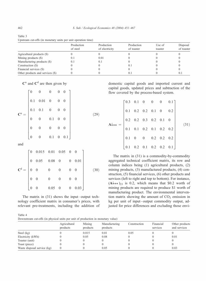
Table 3

Upstream cut-offs (in monetary units per unit operation time)

Production

of steel

Production

of electricity

Production

of toaster

Use of

toaster

Disposal

of toaster

Agricultural products ($) 0 0 0 0 0

Mining products ($) 0.1 0.01 0 0 0

Manufacturing products ($) 0.1 0.1 0 0 0

Construction ($) 0 0 0.1 0 0

Financial services ($) 0 0 0 0 0

Other products and services ($) 0 0 0.1 0 0.1


Cu and Cd are then given by

Cu ¼

0 0 0 0 0

0:1 0:01 0 0 0

0:1 0:1 0 0 0

0 0 0:1 0 0

0 0 0 0 0

0 0 0:1 0 0:1

266666666666666664

377777777777777775

ð29Þ

and

Cd ¼

0 0:015 0:01 0:05 0 0

0 0:05 0:08 0 0 0:01

0 0 0 0 0 0

0 0 0 0 0 0

0 0 0:05 0 0 0:03

26666666666664

37777777777775

ð30Þ

The matrix in (31) shows the input–output tech-

nology coefficient matrix in consumer’s prices, with

relevant pre-treatments, including the addition of

Table 4

Downstream cut-offs (in physical units per unit of production in monetar

Agricultural

products

Mining

products

Man

prod

Steel (kg) 0 0.015 0.01

Electricity (kWh) 0 0.05 0.08

Toaster (unit) 0 0 0

Toast (piece) 0 0 0

Waste disposal service (kg) 0 0 0.05

domestic capital goods and imported current and

capital goods, updated prices and subtraction of the

flow covered by the process-based system.

A***V ¼

0:3 0:1 0 0 0 0:1

0:1 0:2 0:2 0:1 0 0:2

0:2 0:2 0:3 0:2 0:1 0

0:1 0:1 0:2 0:1 0:2 0:2

0:1 0 0 0:2 0:2 0:2

0:1 0:2 0:1 0:2 0:2 0:1

266666666666666664

377777777777777775

ð31Þ

The matrix in (31) is a commodity-by-commodity

aggregated technical coefficient matrix, its row and

column indices being (1) agricultural products, (2)

mining products, (3) manufactured products, (4) con-

struction, (5) financial services, (6) other products and

services (left to right and top to bottom). For instance,

(A***V )23 is 0.2, which means that $0.2 worth of

mining products are required to produce $1 worth of

manufacturing product. The environmental interven-

tion matrix showing the amount of CO2 emission in

kg per unit of input–output commodity output, ad-

justed for price differences and excluding those envi-

y value)

ufacturing

ucts

Construction Financial

services

Other products

and services

0.05 0 0

0 0 0.01

0 0 0

0 0 0

0 0 0.03


ronmental interventions already covered by processes,

is given by

B***V ¼ ½ 0:5 3 2 0:1 0:1 1 �: ð32Þ

Now the process-based LCA system is ready to

be integrated with the input–output table through

upstream and downstream cut-offs. Eq. (27) delivers

the result, using the integrated hybrid system and

taking into consideration the interactions between the

process-based system and the input–output based

system by

q ¼ ½ B B***V �A* �Cd

�Cu I� A***V

24

35�1

y

0

24

35 ¼ 30:015;

ð33Þ

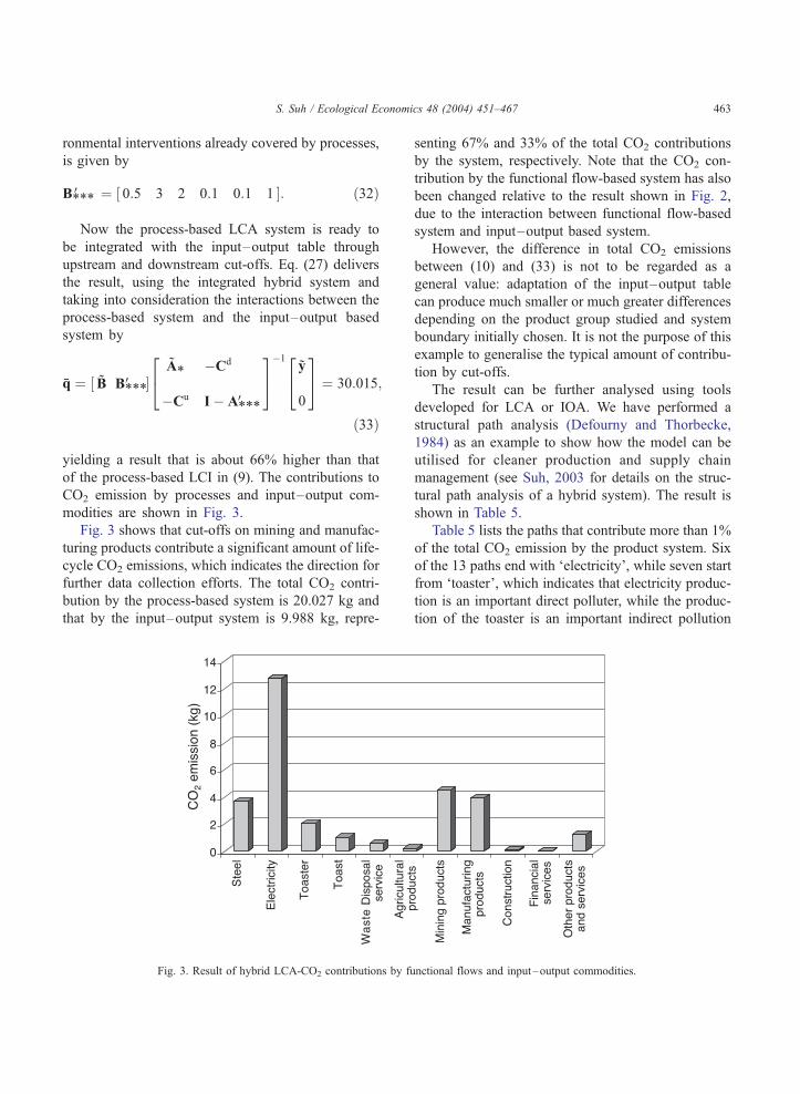
yielding a result that is about 66% higher than that

of the process-based LCI in (9). The contributions to

CO2 emission by processes and input–output com-

modities are shown in Fig. 3.

Fig. 3 shows that cut-offs on mining and manufac-

turing products contribute a significant amount of life-

cycle CO2 emissions, which indicates the direction for

further data collection efforts. The total CO2 contri-

bution by the process-based system is 20.027 kg and

that by the input–output system is 9.988 kg, repre-

Fig. 3. Result of hybrid LCA-CO2 contributions by fu

senting 67% and 33% of the total CO2 contributions

by the system, respectively. Note that the CO2 con-

tribution by the functional flow-based system has also

been changed relative to the result shown in Fig. 2,

due to the interaction between functional flow-based

system and input–output based system.

However, the difference in total CO2 emissions

between (10) and (33) is not to be regarded as a

general value: adaptation of the input–output table

can produce much smaller or much greater differences

depending on the product group studied and system

boundary initially chosen. It is not the purpose of this

example to generalise the typical amount of contribu-

tion by cut-offs.

The result can be further analysed using tools

developed for LCA or IOA. We have performed a

structural path analysis (Defourny and Thorbecke,

1984) as an example to show how the model can be

utilised for cleaner production and supply chain

management (see Suh, 2003 for details on the struc-

tural path analysis of a hybrid system). The result is

shown in Table 5.

Table 5 lists the paths that contribute more than 1%

of the total CO2 emission by the product system. Six

of the 13 paths end with ‘electricity’, while seven start

from ‘toaster’, which indicates that electricity produc-

tion is an important direct polluter, while the produc-

tion of the toaster is an important indirect pollution

nctional flows and input–output commodities.

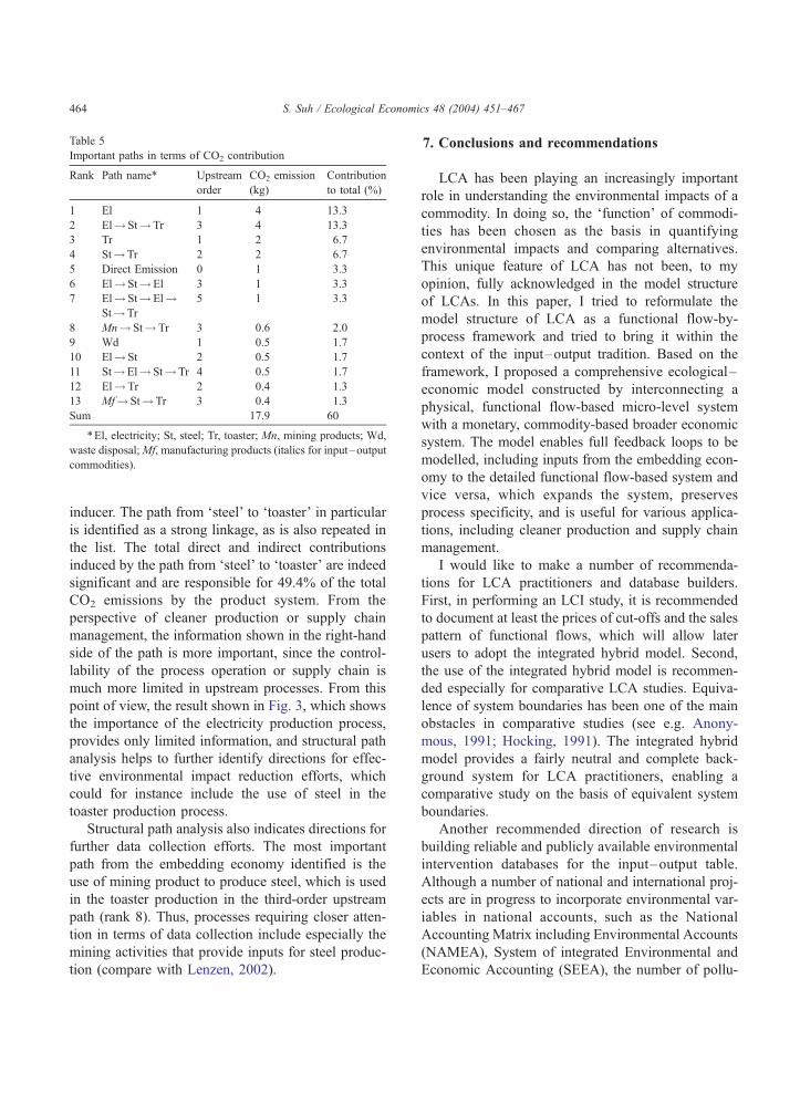
Table 5

Important paths in terms of CO2 contribution

Rank Path name* Upstream

order

CO2 emission

(kg)

Contribution

to total (%)

1 El 1 4 13.3

2 El! St!Tr 3 4 13.3

3 Tr 1 2 6.7

4 St!Tr 2 2 6.7

5 Direct Emission 0 1 3.3

6 El! St!El 3 1 3.3

7 El! St!El!St!Tr

5 1 3.3

8 Mn! St!Tr 3 0.6 2.0

9 Wd 1 0.5 1.7

10 El! St 2 0.5 1.7

11 St!El! St!Tr 4 0.5 1.7

12 El!Tr 2 0.4 1.3

13 Mf! St!Tr 3 0.4 1.3

Sum 17.9 60

*El, electricity; St, steel; Tr, toaster; Mn, mining products; Wd,

waste disposal;Mf, manufacturing products (italics for input–output

commodities).


inducer. The path from ‘steel’ to ‘toaster’ in particular

is identified as a strong linkage, as is also repeated in

the list. The total direct and indirect contributions

induced by the path from ‘steel’ to ‘toaster’ are indeed

significant and are responsible for 49.4% of the total

CO2 emissions by the product system. From the

perspective of cleaner production or supply chain

management, the information shown in the right-hand

side of the path is more important, since the control-

lability of the process operation or supply chain is

much more limited in upstream processes. From this

point of view, the result shown in Fig. 3, which shows

the importance of the electricity production process,

provides only limited information, and structural path

analysis helps to further identify directions for effec-

tive environmental impact reduction efforts, which

could for instance include the use of steel in the

toaster production process.

Structural path analysis also indicates directions for

further data collection efforts. The most important

path from the embedding economy identified is the

use of mining product to produce steel, which is used

in the toaster production in the third-order upstream

path (rank 8). Thus, processes requiring closer atten-

tion in terms of data collection include especially the

mining activities that provide inputs for steel produc-

tion (compare with Lenzen, 2002).

7. Conclusions and recommendations

LCA has been playing an increasingly important

role in understanding the environmental impacts of a

commodity. In doing so, the ‘function’ of commodi-

ties has been chosen as the basis in quantifying

environmental impacts and comparing alternatives.

This unique feature of LCA has not been, to my

opinion, fully acknowledged in the model structure

of LCAs. In this paper, I tried to reformulate the

model structure of LCA as a functional flow-by-

process framework and tried to bring it within the

context of the input–output tradition. Based on the

framework, I proposed a comprehensive ecological–

economic model constructed by interconnecting a

physical, functional flow-based micro-level system

with a monetary, commodity-based broader economic

system. The model enables full feedback loops to be

modelled, including inputs from the embedding econ-

omy to the detailed functional flow-based system and

vice versa, which expands the system, preserves

process specificity, and is useful for various applica-

tions, including cleaner production and supply chain

management.

I would like to make a number of recommenda-

tions for LCA practitioners and database builders.

First, in performing an LCI study, it is recommended

to document at least the prices of cut-offs and the sales

pattern of functional flows, which will allow later

users to adopt the integrated hybrid model. Second,

the use of the integrated hybrid model is recommen-

ded especially for comparative LCA studies. Equiva-

lence of system boundaries has been one of the main

obstacles in comparative studies (see e.g. Anony-

mous, 1991; Hocking, 1991). The integrated hybrid

model provides a fairly neutral and complete back-

ground system for LCA practitioners, enabling a

comparative study on the basis of equivalent system

boundaries.

Another recommended direction of research is

building reliable and publicly available environmental

intervention databases for the input–output table.

Although a number of national and international proj-

ects are in progress to incorporate environmental var-

iables in national accounts, such as the National

Accounting Matrix including Environmental Accounts

(NAMEA), System of integrated Environmental and

Economic Accounting (SEEA), the number of pollu-


tants covered and the resolution of the commodity

classification are rather limited for LCA purposes.

Efforts are also being made by various research groups

to build up publicly available databases (see e.g. Green

Design Initiative, 2002; Nansai et al., 2002; Suh,

2001b; Suh, 2004). For most countries, however,

detailed, sectoral environmental statistics are still not

available. Furthermore, reliable data at the national

level may not be enough for many countries, due to

the proportion of imports. Therefore, efforts should be

made to develop a multi-national database.

The model developed here is also generally appli-

cable to studies on broad interindustry interdepen-

dence in which some part of the system deserves

special attention, including analyses of impact by

consumption, the role of specific technology in con-

nection to its embedding economic system, substance

flow analysis, material flow accounting, etc.

Acknowledgements

I would like to thank Dr. Reinout Heijungs and Dr.

Gjalt Huppes, both at Centre of Environmental

Science (CML) in Leiden University, as well as the

three reviewers, for their valuable comments.

Appendix A

The input–output technology coefficient matrix

derived by the Eq. (11) in the main text includes

some of the functional flows already covered by the

process-based system, especially when (1) a function-

al flow between two processes within a process-based

system involves monetary transaction and (2) both of

the processes belong to industries in the intermediate

part of an input–output table. Therefore, in order to

avoid double counting, these portions of the function-

al flows have to be subtracted from the input–output

based system. If a functional flow satisfies neither of

the two conditions above, the subtraction procedure is

not necessary for the flow.

Since the input–output framework used for the

integrated hybrid model is based on a commodity-by-

commodity technology coefficient matrix, subtraction

of the portions counted double is done at the level of

make and use matrices.

Let us start with the functional flow records

matrix, Z*. If some of the basis periods used for

steady-state approximation are other than 1 year, a

diagonal matrix must be multiplied by the relevant

values to adjust them all to 1 year periods. For our

present calculations, we assume that Z*, Z*u and Z*

d

have been compiled with a basis period of 1 year.

Part of the functional flow-by-process matrix Z* is

extractedtocomposeZ*ksuchthat(Z*

k)ijshows(Z*)ij(Z‹*)ij(Z*)ij if the functional flow of i to process j

satisfies the above mentioned two conditions, and

0 if not. We further divide Z*p into two matrices,

V*p and U*

p , such that

fVp*AðV

p*Þij¼ðZp

*Þji if ðZp�Þji > 0; or 0 otherwiseg:

ðA1Þand

fUp*AðU

p*Þij¼ �ðZp

*Þij if ðZp*Þij < 0; or 0 otherwiseg:

ðA2ÞClearly,

ðVp*Þ

T � Up* ¼ Zp

*: ðA3Þ

Note that V*p is a process-by-functional flow matrix

and U*p is a functional flow-by-process matrix. Let us

further define an commodity-by-functional flow ma-

trix PF such that

fPFAðPFÞij ¼ 1 if functional flow j belongs to

commodity i; or 0 otherwiseg: ðA4Þ

Similarly, a process by input-output industry ma-

trix PP is defined such that

fPPAðPPÞij ¼ 1 if process i belongs to industry j;

or 0 otherwiseg: ðA5Þ

The matrices PF and PP are a functional flow

permutation matrix and a process permutation matrix,

respectively.

Let U** be a commodity-by-industry matrix that

shows the total use of domestic and imported current

commodities and capital by domestic industries, with

updated prices, and let V** be an industry-by-com-

modity matrix that shows the total production of

commodities by domestic industries, with updates

prices. The portion of commodities consumed by the


process-based system is then subtracted from the use

matrix, U** by

U***¼U**�ðmPFUp*PPþ mPFZ

d

* þ Zu

*PPÞ; ðA6Þ

where m denotes the price vector. The portion of

commodities produced by the process-based system is

also subtracted from the make matrix V** by

V*** ¼ V** � mðPPÞTVðPFÞT: ðA7Þ

The commodity-by-commodity technology coeffi-

cient matrix derived by the reduced make and use

matrix in (A6) and (A7), using a relevant model such

as the industry-technology model or the commodity-

technology model, shows the commodity flow rela-

tions, excluding those already covered in the pro-

cess-based system. We use A***V to denote the

commodity-by-commodity input–output technology

coefficient matrix that includes domestic and

imported current products and capital, with prices

updated to current levels, and excluding the portion

of commodity flows already covered by the process-

based system. Similarly, the environmental interven-

tion-by-commodity matrix B**V is reduced to B***Vby subtracting the environmental interventions by

processes that were represented in the input–output

accounts.

References

Anonymous, 1991. Letters. Science 252, 1361–1363.

Ayres, R.U., Ayres, L.W., 1996. Industrial Ecology: Towards Closing

the Materials Cycle. Edward Elgar Publishing, Cheltenham, UK.

Ayres, R.U., Kneese, A.V., 1969. Production, consumption and

externalities. American Economic Review LIX, 282–297.

Bullard, C.W., Pillati, D.A., 1976. Reducing Uncertainty in Energy

Analysis. CAC-doc. no. 205. Center for Advanced Computa-

tion, University of Illinois, Urbana, USA.

Bullard, C.W., Penner, P.S., Pilati, D.A., 1978. Net energy analy-

sis—handbook for combining process and input-output analysis.

Resources and Energy 1, 267–313.

Consoli, F., Allen, D., Bounstead, I., Fava, J., Franklin, W., Jensen,

A.A., de Oude, N., Parirish, R., Perriman, R., Postlethwaite, D.,

Quay, B., Seguin, J., Vigon, B., 1993. Guidelines for Life-Cycle

Assessment: A ‘Code of Practice’ SETAC, Brussels, Belgium.

Defourny, J., Thorbecke, E., 1984. Structural path analysis and

multiplier decomposition within a social accounting matrix

framework. Economic Journal 94, 111–136.

Engelenburg, B.C.W., van Rossum, T.F.M., van Block, K., Vringer,

K., 1994. Calculating the energy requirements of household

purchases: a practical step by step method. Energy Policy 22,

648–656.

Fava, J.A., Denison, R., Jones, B., Curran, M.A., Vigon, B., Selke,

S., Barnum, J., 1991. A Technical Framework for Life-Cycle

Assessment. SETAC, Brussels, Belgium.

Georgescu-Roegen, N., 1971. The Entropy Law and the Economic

Process. Harvard University Press, Cambridge, USA.

Graedel, T.E., Allenby, B.R., 1995. Industrial Ecology. Prentice

Hall, USA.

Green Design Initiative, 2002. Environmental Input–Output Life

Cycle Assessment. Carnegie Mellon University (http://www.

eiolca.net).

Guinee, J.B., Gorree, M., Heijungs, R., Huppes, G., Kleijn, R., van

Oers, L., Wegener Sleeswijk, A., Suh, S., Udo de Haes, H.A., de

Bruijn, J.A., van Duin, R., Huijbregts, M.A.J. (Eds.), 2002.

Handbook on Life Cycle Assessment. Operational Guide to

the ISO Standards. Kluwer Academic Publisher, Dordrecht,

Netherlands.

Heijungs, R., 1994. A generic method for the identification of

options for cleaner products. Ecological Economics 10, 69–81.

Heijungs, R., Frischknecht, R., 1998. A special view on the nature

of the allocation problem. Journal of Life Cycle Assessment 3

(5), 321–332.

Heijungs, R., Suh, S., 2002. Computational Structure of Life

Cycle Assessment. Kluwer Academic Publisher, Dordrecht,

Netherlands.

Hendrickson, C., Horvath, A., Joshi, S., Lave, L., 1998. Econom-

ic input–output models for environmental life cycle assess-

ment. Environmental Science and Technology/News, April 1,

184–190.

Hocking, M.B., 1991. Paper versus polystyrene: a complex choice.

Science 251, 504–505.

International Federation of Institutes for Advanced Studies (IFIAS),

1974. Energy Analysis: Workshop on Methodology and Con-

ventions. Report No. 6, Stockholm.

International Organisation for Standardisation (ISO), 1998. Envi-

ronmental Management –Life Cycle Assessment—Goal and

Scope Definition and Inventory Analysis: ISO 14041. Geneva,

Switzerland.

Isard, W., 1968. Some notes on the linkage of the ecologic and

economic systems. Regional Science Association XXII, 85–96

(Budapest).

Joshi, S., 2000. Product environmental life-cycle assessment using

input–output techniques. Journal of Industrial Ecology 3 (2–3),

95–120.

Konijn, P.J.A., 1994. The Make and Use of Commodities By In-

dustries–on the Compilation of Input–Output Data from the

National Accounts. Ph.D. thesis. University of Twente, Twente,

The Netherlands.

Kop Jansen, P., ten Raa, T., 1990. The choice of model in the

construction of input-output coefficients matrices. International

Economic Review 31, 213–227.

Lancaster, K.J., 1966. A new approach to consumer theory. The

Journal Political Economy 74 (2), 132–157.

Lave, L., Cobas-Flores, E., Hendrickson, C., McMichael, F., 1995.

http:\\www.eiolca.net


Using input–output analysis to estimate economy wide dis-

charges. Environmental Science and Technology 29 (9),

420–426.

Lenzen, M., 2001. A generalized input–output multiplier calculus

for Australia. Economic Systems Research 13 (1), 67–92.

Lenzen, M., 2002. A guide for compiling inventories in hybrid life-

cycle assessments: some Australian results. Journal of Cleaner

Production 10, 545–572.

Leontief, W.W., 1936. Quantitative input and output relations in the

economic system of the United States. The Review of Economic

Statistics 18 (3), 105–125.

Leontief, W.W., 1941. The Structure of American Economy,

1919–1939. An Empirical Application of Equilibrium Analy-

sis. Oxford University Press, New York, USA.

Leontief, W.W., 1970. Environmental repercussions and the eco-

nomic structure: an input–output approach. Review of Econom-

ics and Statistics LII (3), 261–271.

Londero, E., 1999. Secondary products, by-products and the com-

modity technology assumption. Economic Systems Research 11

(2), 195–203.

Marheineke, T., Friedrich, R., Krewitt, W., 1998. Application of a

hybrid—approach to the life cycle inventory analysis of a

freight transport task. Total Life Cycle Conference and Exposi-

tion, Austria.

Moriguchi, Y., Kondo, Y., Shimizu, H., 1993. Analyzing the life

cycle impact of cars: the case of CO2. Industry and Environment

16 (1–2), 42–45.

Nansai, K., Moriguchi, Y., Tohno, S., 2002. Embodied Energy and

Emission Intensity data for Japan using Input–Output Tables

(3EID)—Inventory Data for LCA Center for Global Environ-

mental Research, Japan. In press.

Projektgemeinschaft Lebenswegbilanzen, 1991. Umweltprofille

von Packstoffen und Packmitteln. Methode (Entwurf). ILV,

Munchen, Germany.

Sen, A., 1999. Commodities and Capabilities. Oxford University

Press, Delhi, India.

Steenge, A.E., 1990. The commodity technology revisited—theo-

retical basis and an application to error location in the make-use

framework. Economic Modeling 7, 376–387.

Stone, R., Bacharach, M., Bates, J., 1963. Input–Output Relation-

ships, 1951–1966, Programme for Growth, vol. 3. Chapman

and Hall, London, UK.

Suh, S., 2001a. Generalised calculus of allocation in life cycle

assessment—implications of economic models. CML working

paper. CML, Leiden University, Netherlands.

Suh, S., 2001b. Missing Inventory Estimation Tool (MIET) ver-

sion 2.0 CML, Leiden University, Netherlands (http://www.

leidenuniv.nl/cml/ssp/software/miet).

Suh, S., 2003. Accumulative structural path analysis for life cycle

assessment. CML working paper. CML, Leiden University,

Netherlands.

Suh, S., 2004. A Comprehensive Environmental Data Archive

(CEDA) version 3.0 CML, Leiden University, Netherlands

(http://www.leidenuniv.nl/cml/ssp/software/ceda).

Suh, S., Huppes, G. Techniques in life cycle inventory of a product.

Journal of Cleaner Production (in press).

Suh, S., Huppes, G., 2002. Missing inventory estimation tool using

extended input–output analysis. International Journal of Life

Cycle Assessment 7 (3), 134–140.

Suh, S., Lenzen, M., Treloar, G.J., Hondo, H., Horvath, A., Huppes,

G., Jolliet, O., Klann, U., Krewitt, W., Moriguchi, Y., Munks-

gaard, J., Norris, G., 2004. System boundary selection in life

cycle inventories using hybrid approaches. Environmental Sci-

ence and Technology 38 (3), 657–664.

ten Raa, T., 1988. An alternative treatment of secondary products in

input–output analysis: frustration. Review of Economics and

Statistics 70 (3), 535–538.

ten Raa, T., Chakraborty, D., Small, J.A., 1984. An alternative

treatment of secondary products in input–output analysis. Re-

view of Economics and Statistics 66 (1), 88–97.

Treloar, G., 1997. Extracting embodied energy paths from in-

put–output tables: towards an input–output-based hybrid en-

ergy analysis method. Economic Systems Research 9 (4),

375–391.

US EPA, 1993. Life-Cycle Assessment: Inventory Guidelines and

Principles. EPA/600/R-92/245. US Environmental Protection

Agency (EPA), USA.

Weidema, B.P., 2001. Avoiding co-product allocation in life-cycle

assessment. Journal of Industrial Ecology 4 (3), 39–61.

Wilting, H.C., 1996. An energy perspective on economic activities.

Ph.D. thesis. University of Groningen, Netherlands.

Worster, D., 1994. Natures’ Economy: A History of Ecological

Ideas, 2nd ed. Cambridge University Press, Cambridge, New

York, USA.

http:\\www.leidenuniv.nl\cml\ssp\software\miet

http:\\www.leidenuniv.nl\cml\ssp\software\ceda

Documents

Functions, commodities and environmental impacts in an ecological–economic model