Functions of Several Variables: Limits and Continuityksuweb.kennesaw.edu/~plaval/math2203/funcnD_limcont_slides.pdf · Introduction We extend the notion of limits studied in Calculus

Functions of Several Variables: Limits and Continuity

Philippe B. Laval

KSU

Today

Philippe B. Laval (KSU) Limits and Continuity Today 1 / 24

Introduction

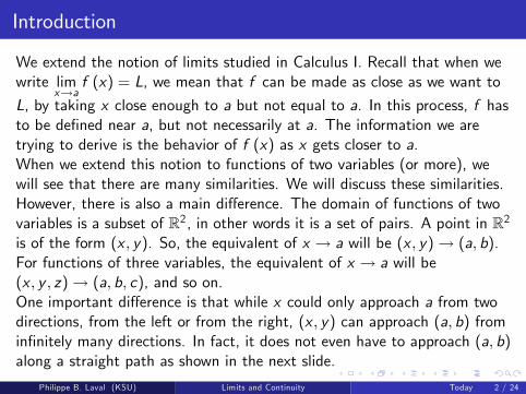
We extend the notion of limits studied in Calculus I. Recall that when wewrite lim

x→af (x) = L, we mean that f can be made as close as we want to

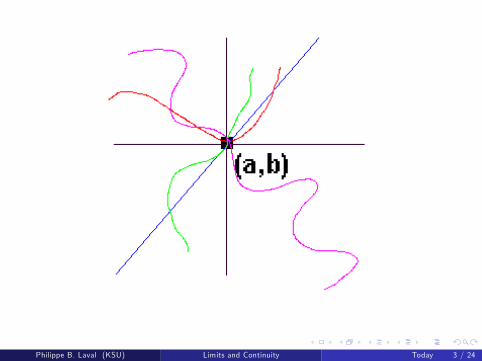
L, by taking x close enough to a but not equal to a. In this process, f hasto be defined near a, but not necessarily at a. The information we aretrying to derive is the behavior of f (x) as x gets closer to a.When we extend this notion to functions of two variables (or more), wewill see that there are many similarities. We will discuss these similarities.However, there is also a main difference. The domain of functions of twovariables is a subset of R2, in other words it is a set of pairs. A point in R2is of the form (x , y). So, the equivalent of x → a will be (x , y)→ (a, b).For functions of three variables, the equivalent of x → a will be(x , y , z)→ (a, b, c), and so on.One important difference is that while x could only approach a from twodirections, from the left or from the right, (x , y) can approach (a, b) frominfinitely many directions. In fact, it does not even have to approach (a, b)along a straight path as shown in the next slide.



Introduction

With functions of one variable, one way to show a limit existed, was toshow that the limit from both directions existed and were equal( limx→a−

f (x) = limx→a+

f (x)). Equivalently, when the limits from the two

directions were not equal, we concluded that the limit did not exist. Forfunctions of several variables, we would have to show that the limit alongevery possible path exist and are the same. The problem is that there areinfinitely many such paths. To show a limit does not exist, it is stillenough to find two paths along which the limits are not equal. In view ofthe number of possible paths, it is not always easy to know which paths totry. We give some suggestions here. You can try the following paths:

1 Horizontal line through (a, b), the equation of such a path is y = b.2 Vertical line through (a, b), the equation of such a path is x = a.3 Any straight line through (a, b) ,the equation of the line with slope mthrough (a, b) is y = mx + b − am.

4 Quadratic paths. For example, a typical quadratic path through (0, 0)is y = x2.


Introduction

While it is important to know how to compute limits, it is also importantto understand what we are trying to accomplish. Like for functions of onevariable, when we compute the limit of a function of several variables at apoint, we are simply trying to study the behavior of that function near thatpoint. The questions we are trying to answer are:

1 Does the function behave nicely near the point in questions? In otherwords, does the function seem to be approaching a single value as itsinput is approaching the point in question?

2 Is the function getting arbitrarily large (going to ∞ or −∞)?3 Does the function behave erratically, that is it does not seem to beapproaching any value?

In the first case, we will say that the limit exists and is equal to the valuethe function seems to be approaching. In the other cases, we will say thatthe limit does not exist.


Definitions

DefinitionWe write lim

(x ,y )→(a,b)f (x , y) = L and we read the limit of f (x , y) as

(x , y) approaches (a, b) is L, if we can make f (x , y) as close as we wantto L, simply by taking (x , y) close enough to (a, b) but not equal to it.

Let us make a few remarks.1 When computing lim

(x ,y )→(a,b)f (x , y), (x , y) is never equal to (a, b). In

fact, f may not even be defined at (a, b). However f must be definedat the points (x , y) we consider as (x , y)→ (a, b).

2 There are several notation for this limit. They all represent the samething, we list them below.

lim(x ,y )→(a,b)

f (x , y) = L

limx→ay→b

f (x , y) = L

f (x , y) approaches L as (x , y) approaches (a, b).


Computing Limits: Numerical Method

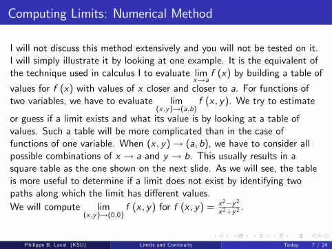
I will not discuss this method extensively and you will not be tested on it.I will simply illustrate it by looking at one example. It is the equivalent ofthe technique used in calculus I to evaluate lim

x→af (x) by building a table of

values for f (x) with values of x closer and closer to a. For functions oftwo variables, we have to evaluate lim

(x ,y )→(a,b)f (x , y). We try to estimate

or guess if a limit exists and what its value is by looking at a table ofvalues. Such a table will be more complicated than in the case offunctions of one variable. When (x , y)→ (a, b), we have to consider allpossible combinations of x → a and y → b. This usually results in asquare table as the one shown on the next slide. As we will see, the tableis more useful to determine if a limit does not exist by identifying twopaths along which the limit has different values.We will compute lim

(x ,y )→(0,0)f (x , y) for f (x , y) = x 2−y 2

x 2+y 2 .


Computing Limits: Numerical Method

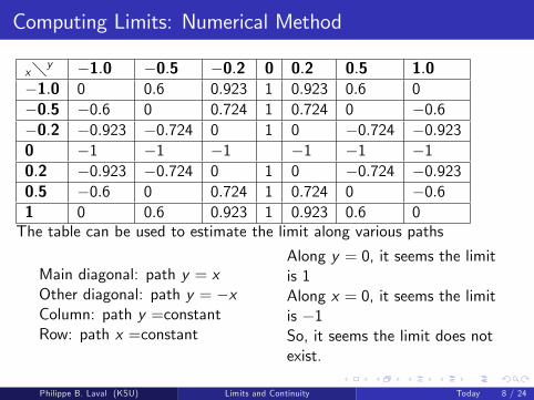
x�y −1.0 −0.5 −0.2 0 0.2 0.5 1.0−1.0 0 0.6 0.923 1 0.923 0.6 0−0.5 −0.6 0 0.724 1 0.724 0 −0.6−0.2 −0.923 −0.724 0 1 0 −0.724 −0.9230 −1 −1 −1 −1 −1 −10.2 −0.923 −0.724 0 1 0 −0.724 −0.9230.5 −0.6 0 0.724 1 0.724 0 −0.61 0 0.6 0.923 1 0.923 0.6 0The table can be used to estimate the limit along various paths

Main diagonal: path y = xOther diagonal: path y = −xColumn: path y =constantRow: path x =constant

Along y = 0, it seems the limitis 1Along x = 0, it seems the limitis −1So, it seems the limit does notexist.


Computing Limits: Analytical Method

Computing limits using the analytical method is computing limits usingthe limit rules and theorems. We will see that these rules and theorems aresimilar to those used with functions of one variable. We present themwithout proof, and illustrate them with examples.We list these properties for functions of two variables. Similar propertieshold for functions of more variables. Let us assume that L, M, c and k arereal numbers and that lim

(x ,y )→(a,b)f (x , y) = L and lim

(x ,y )→(a,b)g (x , y) = M.

Then, the following are true:



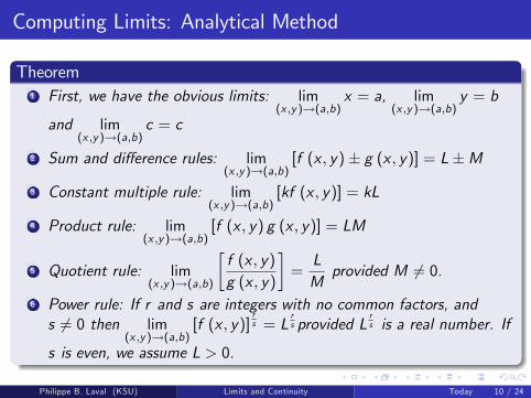
Theorem1 First, we have the obvious limits: lim

(x ,y )→(a,b)x = a, lim

(x ,y )→(a,b)y = b

and lim(x ,y )→(a,b)

c = c

2 Sum and difference rules: lim(x ,y )→(a,b)

[f (x , y)± g (x , y)] = L±M

3 Constant multiple rule: lim(x ,y )→(a,b)

[kf (x , y)] = kL

4 Product rule: lim(x ,y )→(a,b)

[f (x , y) g (x , y)] = LM

5 Quotient rule: lim(x ,y )→(a,b)

[f (x , y)g (x , y)

]=LMprovided M 6= 0.

6 Power rule: If r and s are integers with no common factors, ands 6= 0 then lim

(x ,y )→(a,b)[f (x , y)]

rs = L

rs provided L

rs is a real number. If

s is even, we assume L > 0.



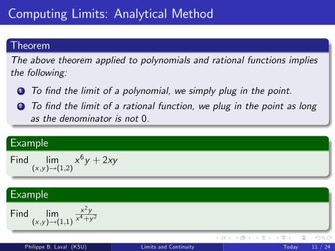
TheoremThe above theorem applied to polynomials and rational functions impliesthe following:

1 To find the limit of a polynomial, we simply plug in the point.2 To find the limit of a rational function, we plug in the point as longas the denominator is not 0.

Example

Find lim(x ,y )→(1,2)

x6y + 2xy

Example


x 2yx 4+y 2



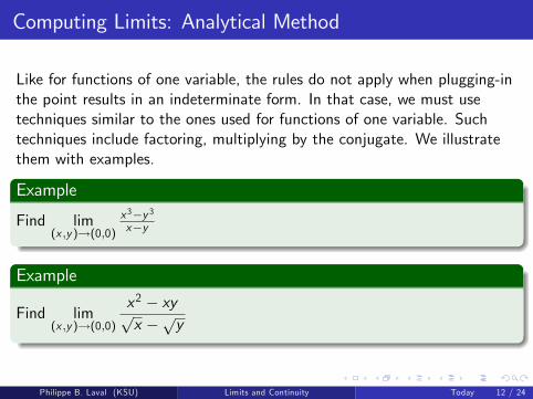
Like for functions of one variable, the rules do not apply when plugging-inthe point results in an indeterminate form. In that case, we must usetechniques similar to the ones used for functions of one variable. Suchtechniques include factoring, multiplying by the conjugate. We illustratethem with examples.

Example


x 3−y 3x−y

Example


x2 − xy√x −√y


Limit Along a Path

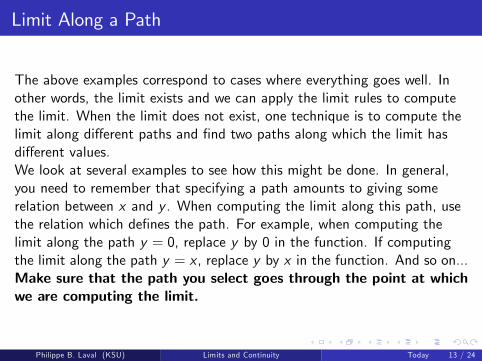
The above examples correspond to cases where everything goes well. Inother words, the limit exists and we can apply the limit rules to computethe limit. When the limit does not exist, one technique is to compute thelimit along different paths and find two paths along which the limit hasdifferent values.We look at several examples to see how this might be done. In general,you need to remember that specifying a path amounts to giving somerelation between x and y . When computing the limit along this path, usethe relation which defines the path. For example, when computing thelimit along the path y = 0, replace y by 0 in the function. If computingthe limit along the path y = x , replace y by x in the function. And so on...Make sure that the path you select goes through the point at whichwe are computing the limit.


Limit Along a Path

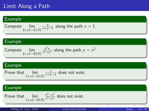
Example

Compute lim(x ,y )→(1,0)

yx+y−1 along the path x = 1.

Example

Compute lim(x ,y )→(0,0)

x 2yx 4+y 2 along the path y = x

2.

Example

Prove that lim(x ,y )→(1,0)

yx+y−1 does not exist.

Example


x 2−y 2x 2+y 2 does not exist.


Limit Along a Path

Example


xyx 2+y 2 does not exist.

Example


x 2yx 4+y 2 does not exist.


Additional Techniques: Change of Coordinates

Example

Using polar coordinates, find lim(x ,y )→(0,0)

x 3+y 3

x 2+y 2 .


Additional Techniques: Squeeze Theorem

We give two versions of the squeeze theorem and illustrate them withexamples. The diffi culty with the squeeze theorem is that we must suspectwhat the limit is. One way to know this is to compute the limit alongvarious paths. As we saw earlier, if we find two paths along which the limitis different, we can conclude the limit does not exist. On the other hand, ifwe try several paths and we always get the same answer for the limit, wemight suspect the limit exists. We then use the squeeze theorem to try toprove it.

TheoremSuppose that |f (x , y)− L| ≤ g (x , y) for every (x , y) inside a diskcentered at (a, b) ,except maybe at (a, b). If lim

(x ,y )→(a,b)g (x , y) = 0 then

lim(x ,y )→(a,b)

f (x , y) = L.



Example


f (x , y) for f (x , y) = x 2yx 2+y 2 .

Example


f (x , y) for f (x , y) = (x−1)2 ln x(x−1)2+y 2 .



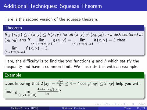
Here is the second version of the squeeze theorem.

TheoremIf g (x , y) ≤ f (x , y) ≤ h (x , y) for all (x , y) 6= (x0, y0) in a disk centered at(x0, y0) and if lim

(x ,y )→(x0,y0)g (x , y) = lim

(x ,y )→(x0,y0)h (x , y) = L then

lim(x ,y )→(x0,y0)

f (x , y) = L.

Here, the diffi culty is to find the two functions g and h which satisfy theinequality and have a common limit. We illustrate this with an example.

Example

Does knowing that 2 |xy | − x 2y 2

6 ≤ 4− 4 cos√|xy | ≤ 2 |xy | help you with

finding lim(x ,y )→(0,0)

4−4 cos√|xy |

|xy | ?


Continuity

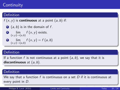
Definitionf (x , y) is continuous at a point (a, b) if:

1 (a, b) is in the domain of f .2 lim(x ,y )→(a,b)

f (x , y) exists.

3 lim(x ,y )→(a,b)

f (x , y) = f (a, b)

DefinitionIf a function f is not continuous at a point (a, b), we say that it isdiscontinuous at (a, b).

DefinitionWe say that a function f is continuous on a set D if it is continuous atevery point in D.


Continuity

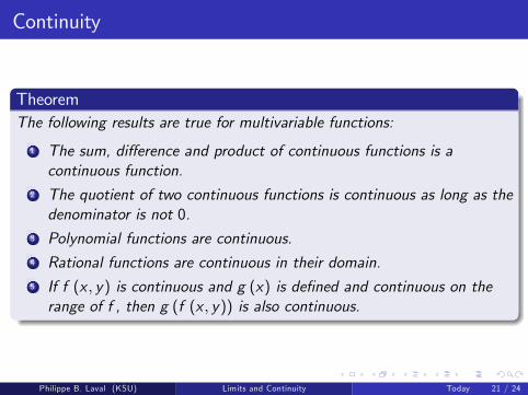
TheoremThe following results are true for multivariable functions:

1 The sum, difference and product of continuous functions is acontinuous function.

2 The quotient of two continuous functions is continuous as long as thedenominator is not 0.

3 Polynomial functions are continuous.4 Rational functions are continuous in their domain.5 If f (x , y) is continuous and g (x) is defined and continuous on therange of f , then g (f (x , y)) is also continuous.


Continuity

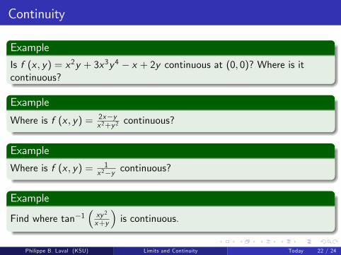
Example

Is f (x , y) = x2y + 3x3y4 − x + 2y continuous at (0, 0)? Where is itcontinuous?

Example

Where is f (x , y) = 2x−yx 2+y 2 continuous?

Example

Where is f (x , y) = 1x 2−y continuous?

Example

Find where tan−1(xy 2

x+y

)is continuous.


Continuity

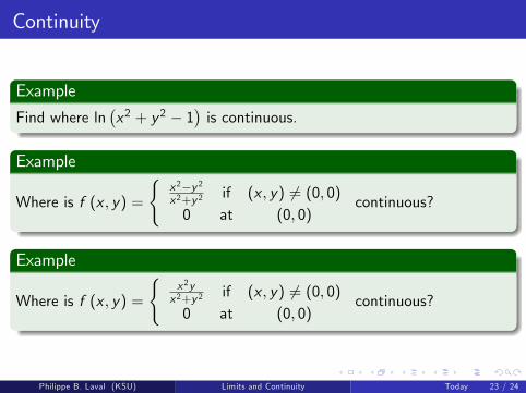
Example

Find where ln(x2 + y2 − 1

)is continuous.

Example

Where is f (x , y) =

{x 2−y 2x 2+y 2 if (x , y) 6= (0, 0)0 at (0, 0)

continuous?

Example

Where is f (x , y) =

{x 2yx 2+y 2 if (x , y) 6= (0, 0)0 at (0, 0)

continuous?


Exercises

See the problems at the end of my notes on limits and continuity offunctions of two or more variables.Review the notion of the derivative from Calculus I.


http://science.kennesaw.edu/~plaval/math2203/funcnD_limcont.pdf

http://science.kennesaw.edu/~plaval/math2203/funcnD_limcont.pdf

Documents

Functions of Several Variables: Limits and Continuityksuweb.kennesaw.edu/~plaval/math2203/funcnD_limcont_slides.pdf · Introduction We extend the notion of limits studied in Calculus