Fundamental Sampling Distributions and Data Descriptions ENGSTAT Notes of AM Fillone, De La Salle University-Manila

Fundamental Sampling Distributions and Data Descriptions

ENGSTAT Notes of AM Fillone, De La Salle University-Manila

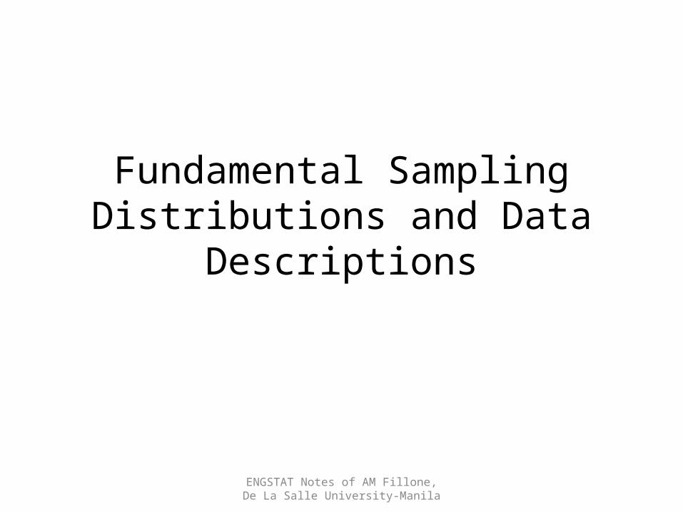
Population – the totality of observations with which we are concerned, whether their number be finite or infinite-Statisticians uses the term to refer to observations relevant to anything of interest, whether it be groups of people, animals, or all possible outcomes from some complicated biological or engineering system

Definition 8.1 A population consists of the totality of the observations with which we are concerned.

Definition 8.2 A sample is a subset of a population.

Definition 8.3 Let X1, X2, …, Xn be n independent random variables, each having the same probability distribution f(x). Define X1, X2, …, Xn to be a random sample of size n from the population f(x) and write its joint probability distribution as

f(x1, x2, …, xn) = f(x1)f(x2) … f(xn)


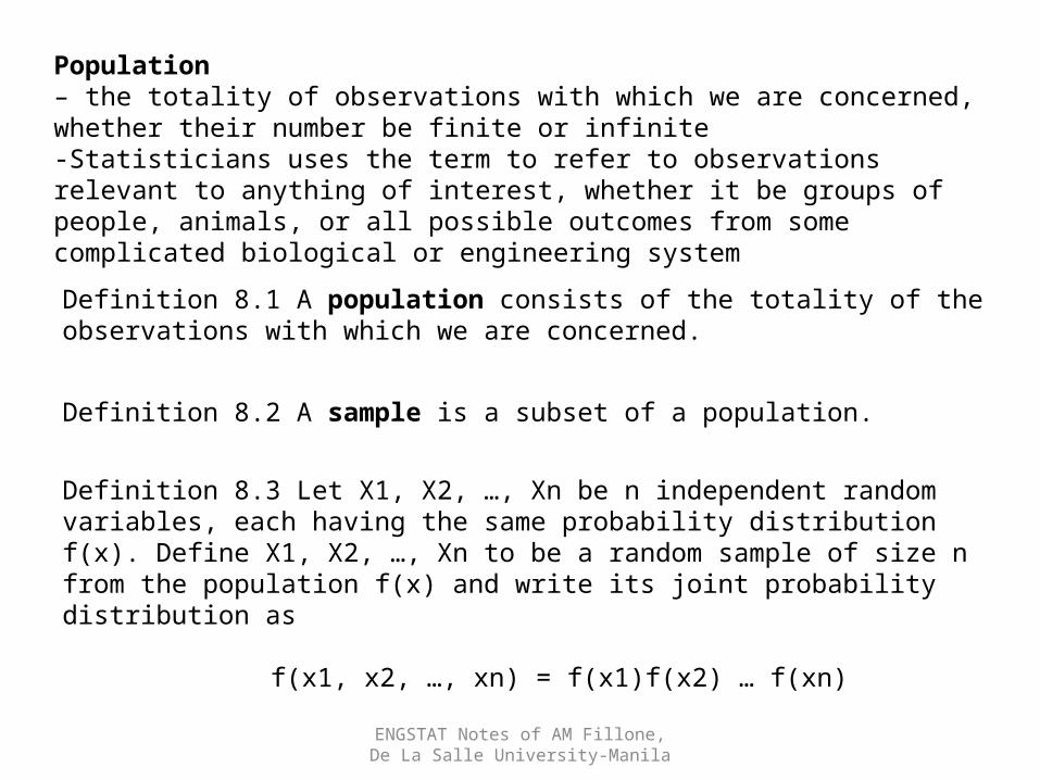
Some Important StatisticsDefinition 8.4: Any function of the random variables constituting a random sample is called a statistic.Definition 8.5: If X1, X2, …, Xn represent a random sample of size n, then the sample mean is defined by the statistic.

Definition 8.6: If X1, X2, …, Xn represent a random sample of size n, then the sample variance is defined by the statistic

Theorem 8.1: If S2 is the variance of a random sample of size n, we may write

Definition 8.7: The sample standard deviation, denoted by S, is the positive square root of the sample variance.


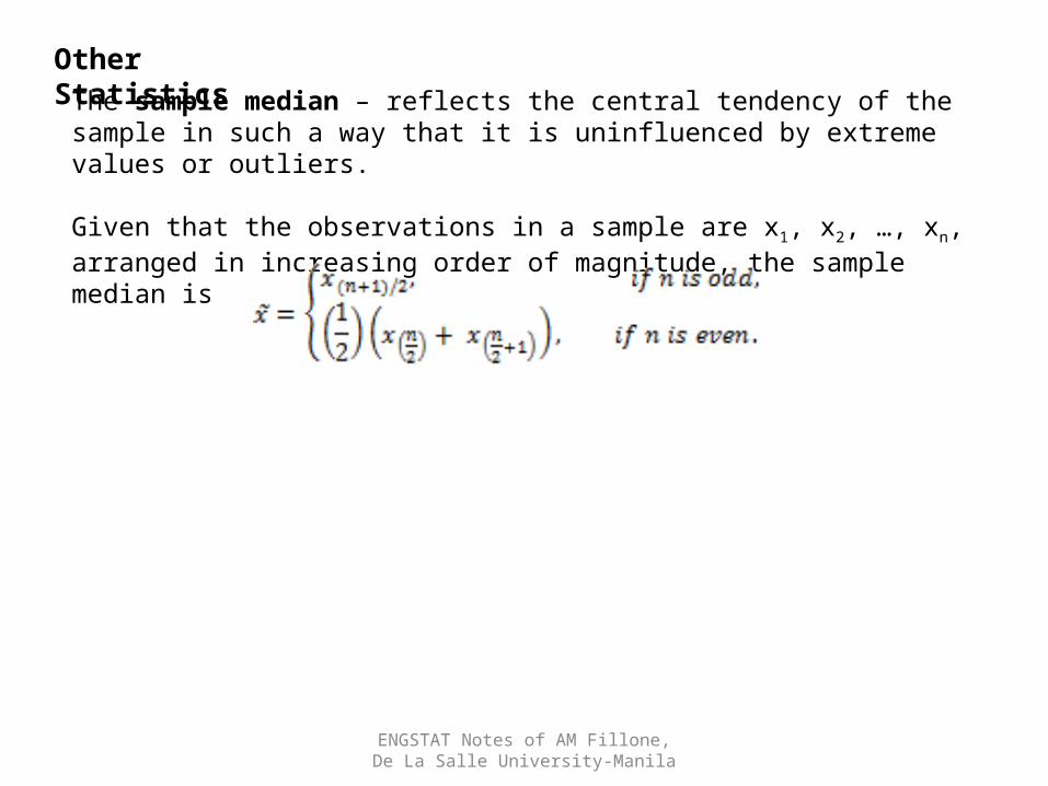
Other StatisticsThe sample median – reflects the central tendency of the sample in such a way that it is uninfluenced by extreme values or outliers.

Given that the observations in a sample are x1, x2, …, xn, arranged in increasing order of magnitude, the sample median is


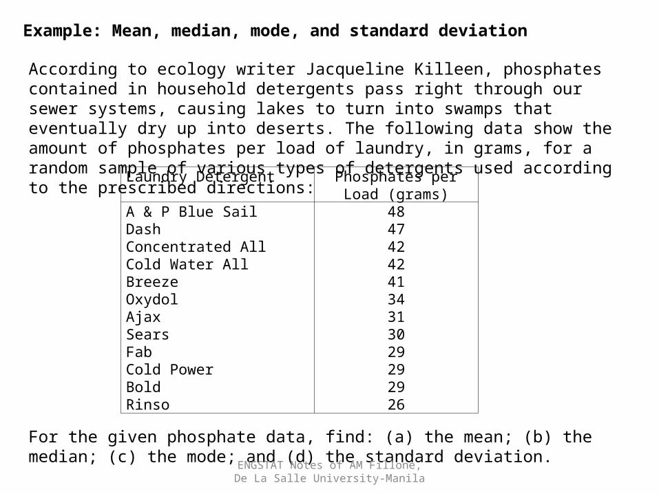
Example: Mean, median, mode, and standard deviation

According to ecology writer Jacqueline Killeen, phosphates contained in household detergents pass right through our sewer systems, causing lakes to turn into swamps that eventually dry up into deserts. The following data show the amount of phosphates per load of laundry, in grams, for a random sample of various types of detergents used according to the prescribed directions:

Laundry Detergent Phosphates per Load (grams)

A & P Blue SailDashConcentrated AllCold Water AllBreezeOxydolAjaxSearsFabCold PowerBoldRinso

484742424134313029292926

For the given phosphate data, find: (a) the mean; (b) the median; (c) the mode; and (d) the standard deviation. ENGSTAT Notes of AM Fillone, De La Salle

University-Manila

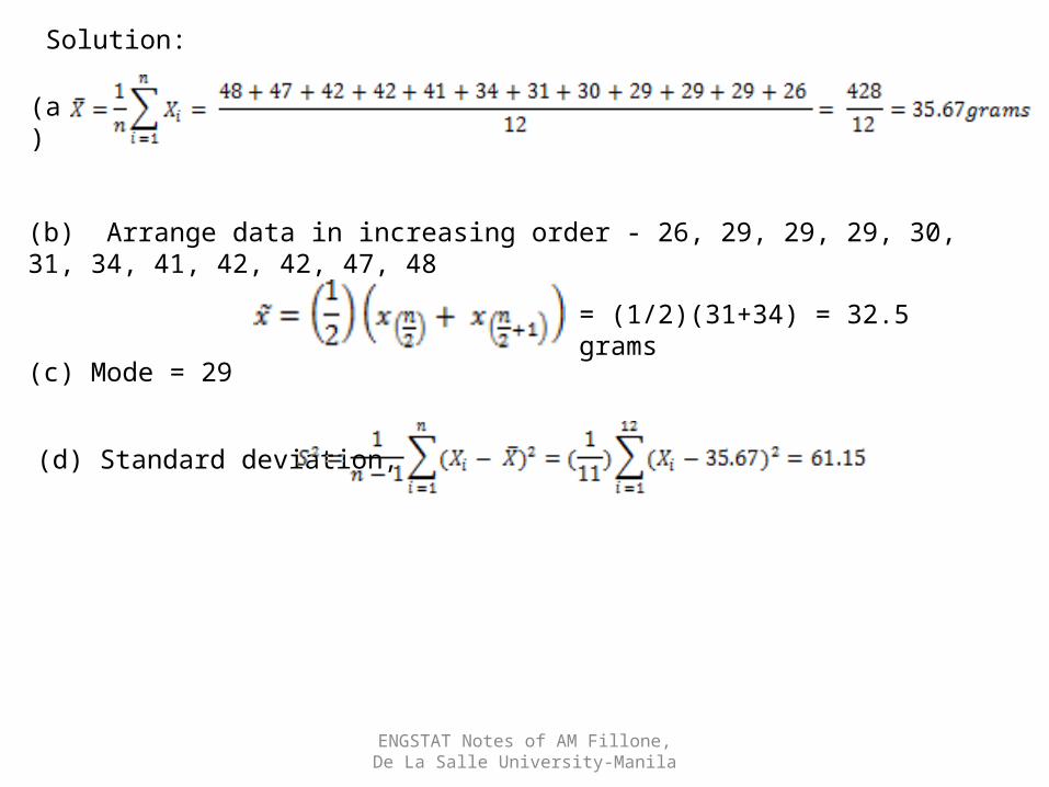
Solution:

(a)

(b) Arrange data in increasing order - 26, 29, 29, 29, 30, 31, 34, 41, 42, 42, 47, 48

= (1/2)(31+34) = 32.5 grams

(c) Mode = 29

(d) Standard deviation,


Data Displays and Graphical Methods

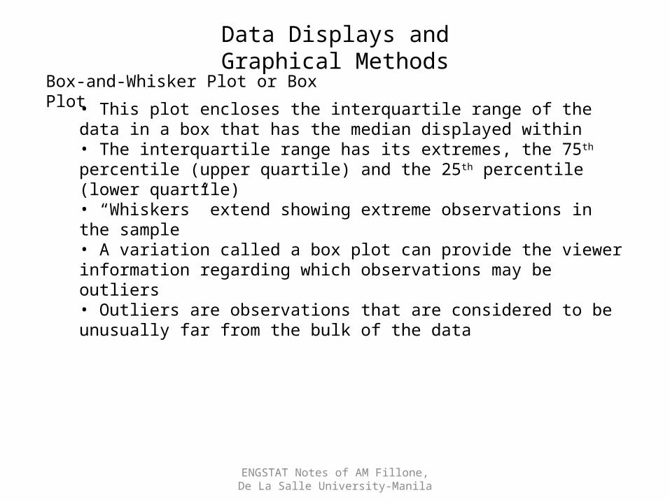
Box-and-Whisker Plot or Box Plot

• This plot encloses the interquartile range of the data in a box that has the median displayed within• The interquartile range has its extremes, the 75th percentile (upper quartile) and the 25th percentile (lower quartile)• “Whiskers” extend showing extreme observations in the sample• A variation called a box plot can provide the viewer information regarding which observations may be outliers• Outliers are observations that are considered to be unusually far from the bulk of the data


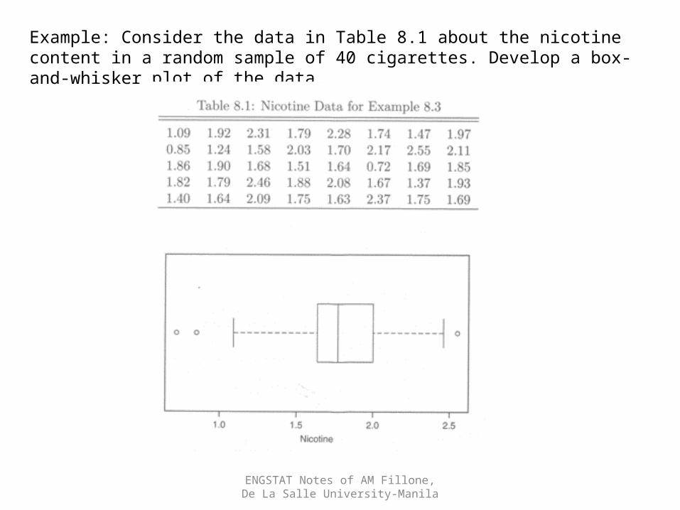
Example: Consider the data in Table 8.1 about the nicotine content in a random sample of 40 cigarettes. Develop a box-and-whisker plot of the data.


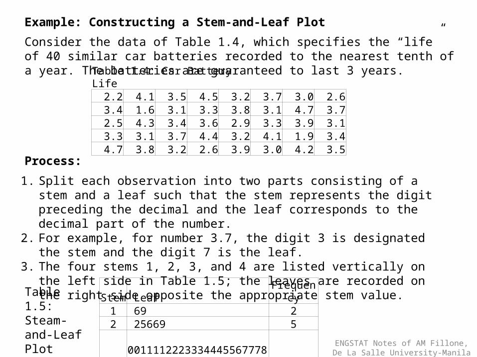
Example: Constructing a Stem-and-Leaf Plot

Consider the data of Table 1.4, which specifies the “life” of 40 similar car batteries recorded to the nearest tenth of a year. The batteries are guaranteed to last 3 years.

Process:

1. Split each observation into two parts consisting of a stem and a leaf such that the stem represents the digit preceding the decimal and the leaf corresponds to the decimal part of the number.

2. For example, for number 3.7, the digit 3 is designated the stem and the digit 7 is the leaf.

3. The four stems 1, 2, 3, and 4 are listed vertically on the left side in Table 1.5; the leaves are recorded on the right side opposite the appropriate stem value.

Table 1.4: Car Battery Life2.2 4.1 3.5 4.5 3.2 3.7 3.0 2.63.4 1.6 3.1 3.3 3.8 3.1 4.7 3.72.5 4.3 3.4 3.6 2.9 3.3 3.9 3.13.3 3.1 3.7 4.4 3.2 4.1 1.9 3.44.7 3.8 3.2 2.6 3.9 3.0 4.2 3.5

Stem Leaf Frequency1 69 22 25669 53 0011112223334445567778899 254 11234577 8 ENGSTAT Notes of AM Fillone, De La Salle

University-Manila

Table 1.5: Steam-and-Leaf Plot

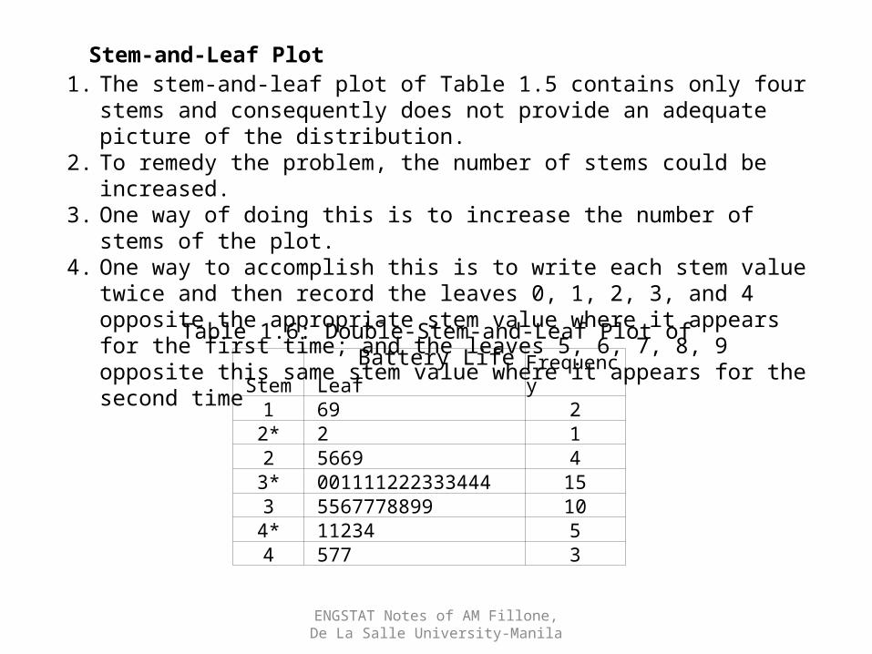
Stem-and-Leaf Plot1. The stem-and-leaf plot of Table 1.5 contains only four stems and consequently

does not provide an adequate picture of the distribution.2. To remedy the problem, the number of stems could be increased.3. One way of doing this is to increase the number of stems of the plot.4. One way to accomplish this is to write each stem value twice and then record the

leaves 0, 1, 2, 3, and 4 opposite the appropriate stem value where it appears for the first time; and the leaves 5, 6, 7, 8, 9 opposite this same stem value where it appears for the second time

Stem Leaf Frequency1 69 2

2* 2 12 5669 4

3* 001111222333444 153 5567778899 10

4* 11234 54 577 3

Table 1.6: Double-Stem-and-Leaf Plot of Battery Life


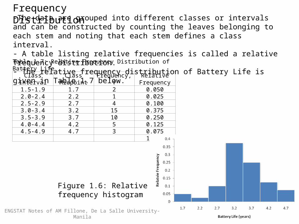
Frequency Distribution-The data are grouped into different classes or intervals and can be constructed by counting the leaves belonging to each stem and noting that each stem defines a class interval.- A table listing relative frequencies is called a relative frequency distribution.- The relative frequency distribution of Battery Life is given in Table 1.7 below. Table 1.7: Relative Frequency Distribution of Battery Life

Class Interval Class Midpoint Frequency, fRelative

Frequency1.5-1.9 1.7 2 0.0502.0-2.4 2.2 1 0.0252.5-2.9 2.7 4 0.1003.0-3.4 3.2 15 0.3753.5-3.9 3.7 10 0.2504.0-4.4 4.2 5 0.1254.5-4.9 4.7 3 0.075

1.000

Figure 1.6: Relative frequency histogram


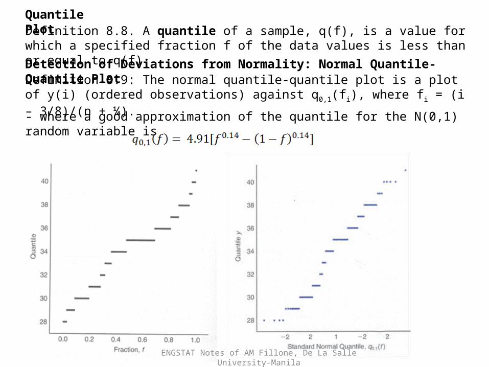
Definition 8.8. A quantile of a sample, q(f), is a value for which a specified fraction f of the data values is less than or equal to q(f).

Quantile Plot

Definition 8.9: The normal quantile-quantile plot is a plot of y(i) (ordered observations) against q0,1(fi), where fi = (i – 3/8)/(n + ¼).


Detection of Deviations from Normality: Normal Quantile-Quantile Plot

- where a good approximation of the quantile for the N(0,1) random variable is

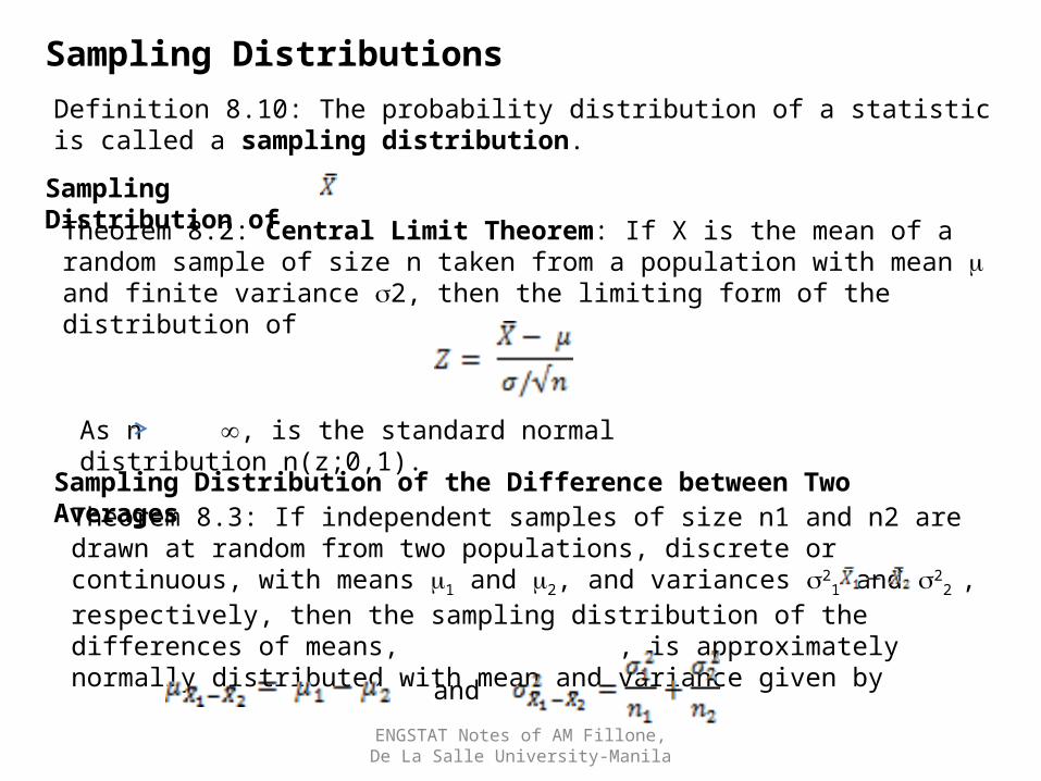
Sampling DistributionsDefinition 8.10: The probability distribution of a statistic is called a sampling distribution.

Theorem 8.2: Central Limit Theorem: If X is the mean of a random sample of size n taken from a population with mean and finite variance 2, then the limiting form of the distribution of

As n , is the standard normal distribution n(z;0,1).

Sampling Distribution of

Sampling Distribution of the Difference between Two AveragesTheorem 8.3: If independent samples of size n1 and n2 are drawn at random from two populations, discrete or continuous, with means 1 and 2, and variances 2

1 and 22 ,

respectively, then the sampling distribution of the differences of means, , is approximately normally distributed with mean and variance given by

and


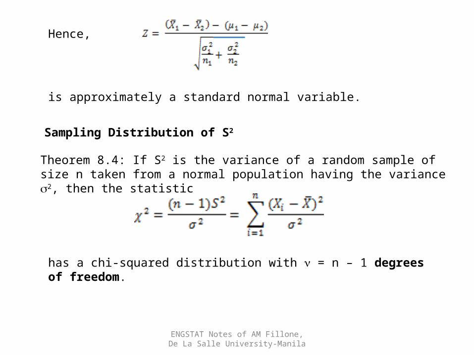
Hence,

is approximately a standard normal variable.

Sampling Distribution of S2

Theorem 8.4: If S2 is the variance of a random sample of size n taken from a normal population having the variance 2, then the statistic

has a chi-squared distribution with = n – 1 degrees of freedom.


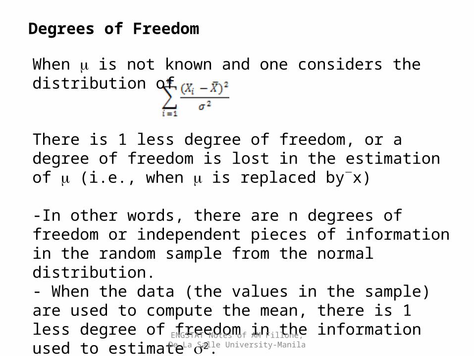
Degrees of Freedom

When is not known and one considers the distribution of

There is 1 less degree of freedom, or a degree of freedom is lost in the estimation of (i.e., when is replaced byx)

-In other words, there are n degrees of freedom or independent pieces of information in the random sample from the normal distribution. - When the data (the values in the sample) are used to compute the mean, there is 1 less degree of freedom in the information used to estimate 2.


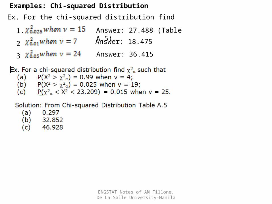
Examples: Chi-squared Distribution

Ex. For the chi-squared distribution find

1.

2.

3.

Answer: 27.488 (Table A.5)

Answer: 18.475

Answer: 36.415


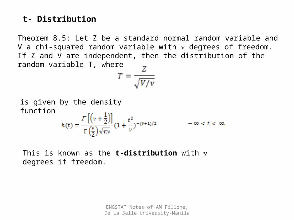
t- Distribution

Theorem 8.5: Let Z be a standard normal random variable and V a chi-squared random variable with degrees of freedom. If Z and V are independent, then the distribution of the random variable T, where

is given by the density function

This is known as the t-distribution with degrees if freedom.


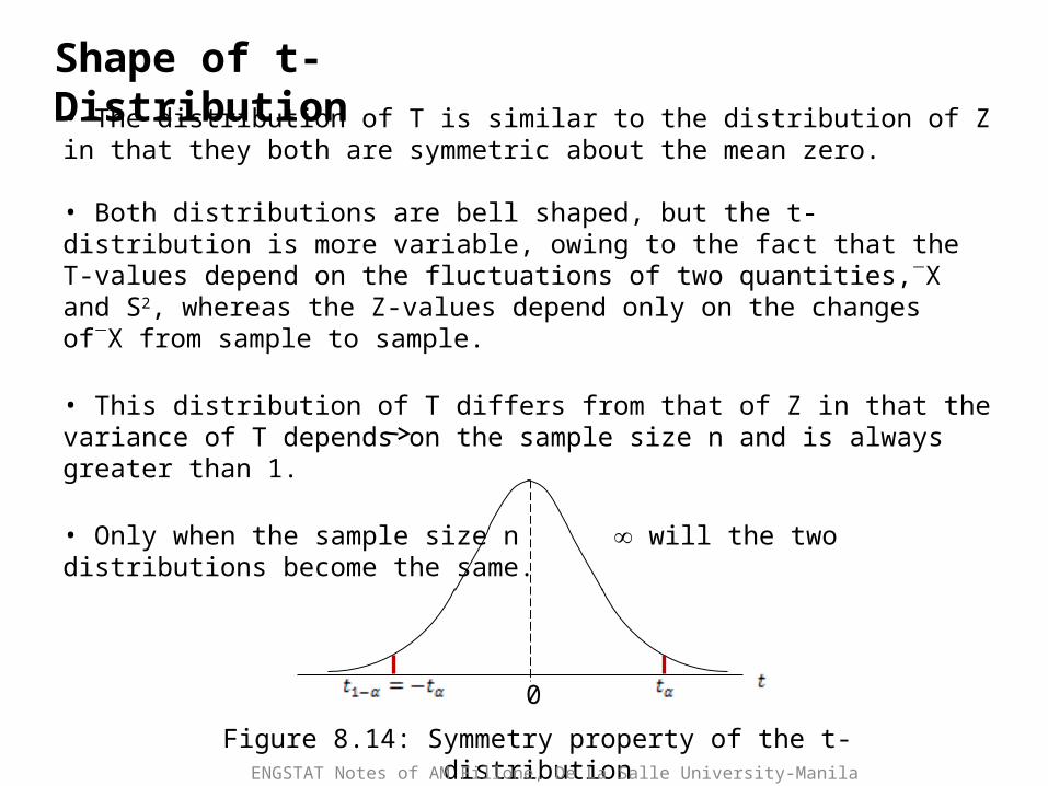
Shape of t-Distribution• The distribution of T is similar to the distribution of Z in that they both are symmetric about the mean zero.

• Both distributions are bell shaped, but the t-distribution is more variable, owing to the fact that the T-values depend on the fluctuations of two quantities,X and S2, whereas the Z-values depend only on the changes ofX from sample to sample.

• This distribution of T differs from that of Z in that the variance of T depends on the sample size n and is always greater than 1.

• Only when the sample size n will the two distributions become the same.

Figure 8.14: Symmetry property of the t-distribution

0


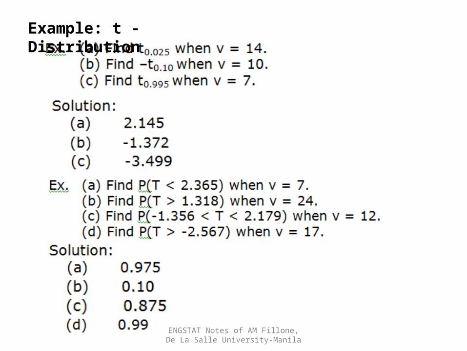
Example: t - Distribution


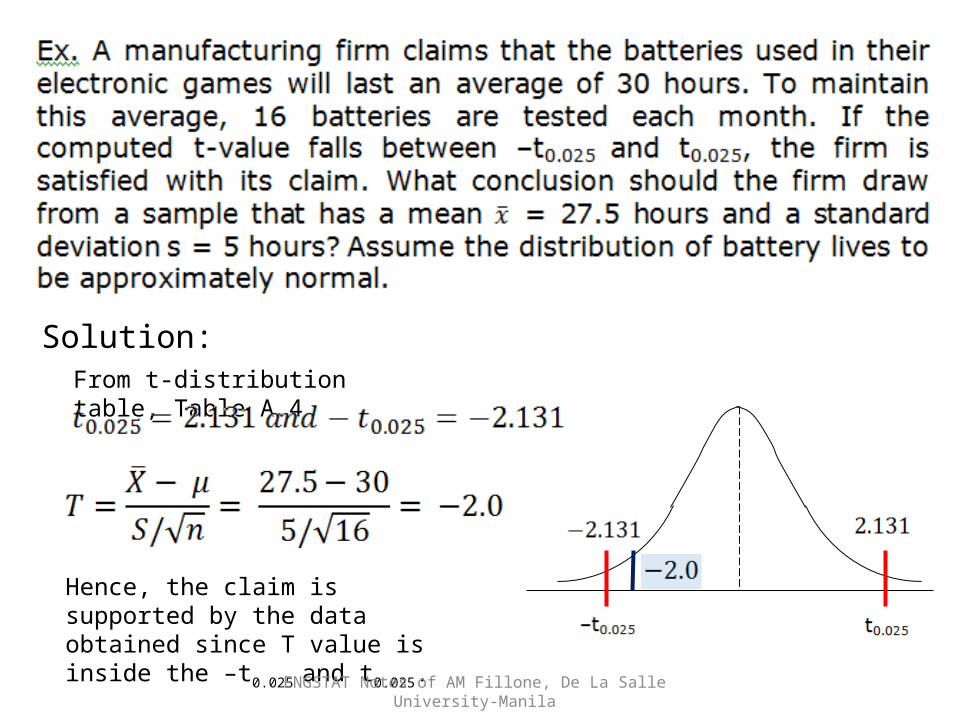
Solution:

Hence, the claim is supported by the data obtained since T value is inside the –t0.025 and t0.025.


From t-distribution table, Table A.4

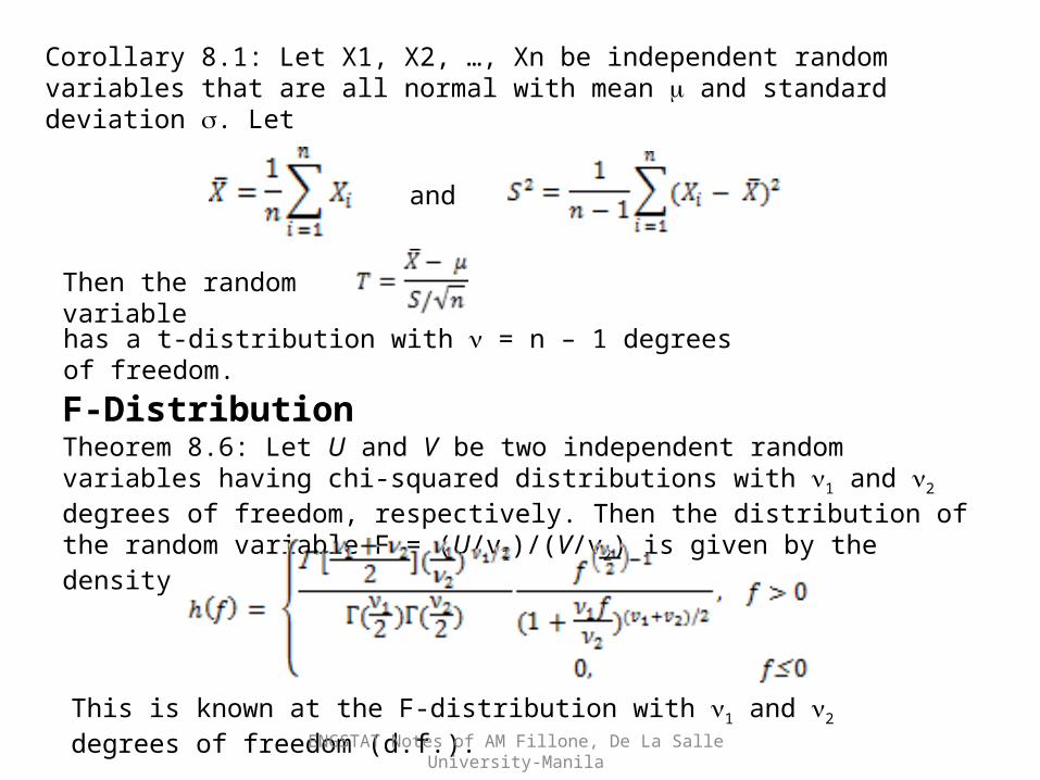
Corollary 8.1: Let X1, X2, …, Xn be independent random variables that are all normal with mean and standard deviation . Let

and

Then the random variable

has a t-distribution with = n – 1 degrees of freedom.

F-DistributionTheorem 8.6: Let U and V be two independent random variables having chi-squared distributions with 1 and 2 degrees of freedom, respectively. Then the distribution of the random variable F = (U/v1)/(V/v2) is given by the density

This is known at the F-distribution with 1 and 2 degrees of freedom (d.f.).


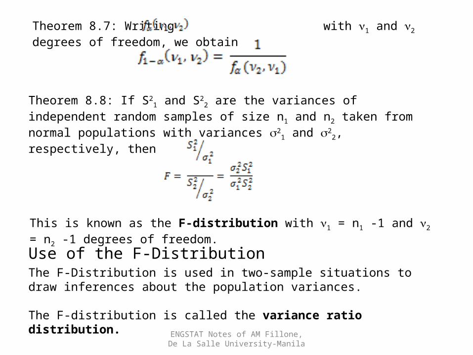
Theorem 8.7: Writing with 1 and 2 degrees of freedom, we obtain

Theorem 8.8: If S21 and S2

2 are the variances of independent random samples of size n1 and n2 taken from normal populations with variances 2

1 and 22,

respectively, then

This is known as the F-distribution with 1 = n1 -1 and 2 = n2 -1 degrees of freedom.

Use of the F-DistributionThe F-Distribution is used in two-sample situations to draw inferences about the population variances.

The F-distribution is called the variance ratio distribution.ENGSTAT Notes of AM Fillone, De La Salle

University-Manila

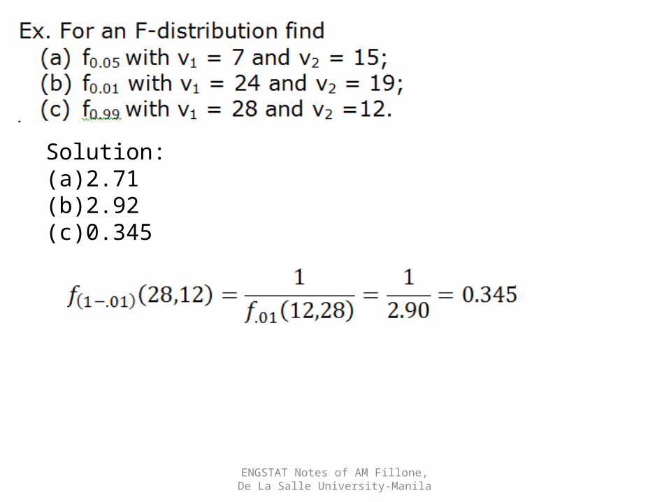
Solution:(a)2.71(b)2.92(c)0.345


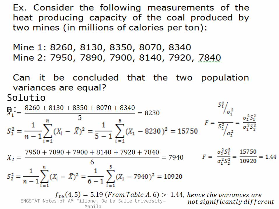
Solution:


Documents

Fundamental Sampling Distributions and Data Descriptions ENGSTAT Notes of AM Fillone, De La Salle University-Manila