Embed Size (px)
Citation preview
Fundamentals of Hypothesis Testing
James H. Steiger
Department of Psychology and Human DevelopmentVanderbilt University
James H. Steiger (Vanderbilt University) 1 / 30
Fundamentals of Hypothesis Testing1 Introduction
2 The Binomial Distribution
Definition and an Example
Derivation of the Binomial Distribution Formula
The Binomial Distribution as a Sampling Distribution
3 Hypothesis Testing
4 One-Tailed vs. Two-Tailed Tests
5 Power of a Statistical Test
6 A General Approach to Power Calculation
Factors Affecting Power: A General Perspective
James H. Steiger (Vanderbilt University) 2 / 30
Introduction
Introduction
In this module, we review the basics of hypothesis testing.
We shall develop the binomial distribution formulas, show how theylead to some important sampling distributions, and then investigatethe key principles of hypothesis testing.
James H. Steiger (Vanderbilt University) 3 / 30
Introduction
Introduction
In this module, we review the basics of hypothesis testing.
We shall develop the binomial distribution formulas, show how theylead to some important sampling distributions, and then investigatethe key principles of hypothesis testing.
James H. Steiger (Vanderbilt University) 3 / 30
The Binomial Distribution Definition and an Example
The Binomial Distribution
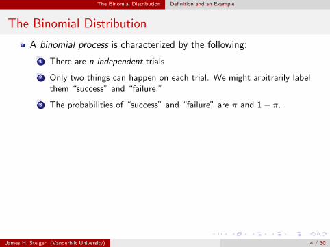
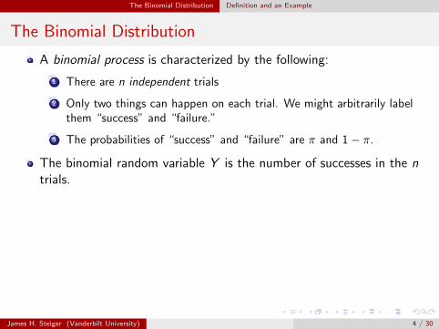
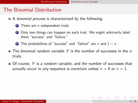
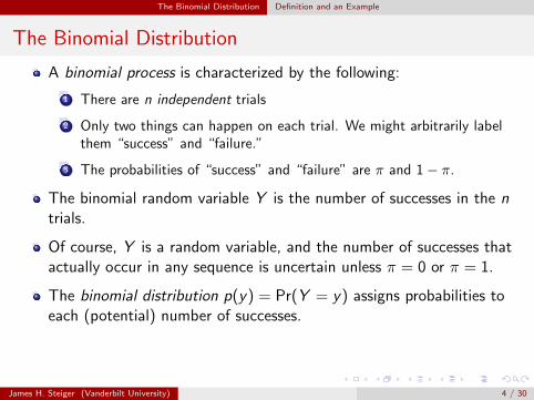
A binomial process is characterized by the following:
1 There are n independent trials
2 Only two things can happen on each trial. We might arbitrarily labelthem “success” and “failure.”
3 The probabilities of “success” and “failure” are π and 1− π.
The binomial random variable Y is the number of successes in the ntrials.
Of course, Y is a random variable, and the number of successes thatactually occur in any sequence is uncertain unless π = 0 or π = 1.
The binomial distribution p(y) = Pr(Y = y) assigns probabilities toeach (potential) number of successes.
James H. Steiger (Vanderbilt University) 4 / 30
The Binomial Distribution Definition and an Example
The Binomial Distribution
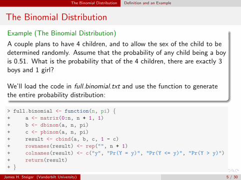
Example (The Binomial Distribution)
A couple plans to have 4 children, and to allow the sex of the child to bedetermined randomly. Assume that the probability of any child being a boyis 0.51. What is the probability that of the 4 children, there are exactly 3boys and 1 girl?
We’ll load the code in full.binomial.txt and use the function to generatethe entire probability distribution:
> full.binomial <- function(n, pi) {+ a <- matrix(0:n, n + 1, 1)
+ b <- dbinom(a, n, pi)
+ c <- pbinom(a, n, pi)
+ result <- cbind(a, b, c, 1 - c)
+ rownames(result) <- rep("", n + 1)
+ colnames(result) <- c("y", "Pr(Y = y)", "Pr(Y <= y)", "Pr(Y > y)")
+ return(result)
+ }James H. Steiger (Vanderbilt University) 5 / 30
The Binomial Distribution Definition and an Example
The Binomial Distribution
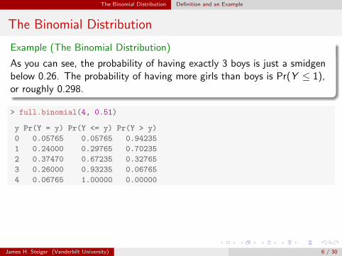
Example (The Binomial Distribution)
As you can see, the probability of having exactly 3 boys is just a smidgenbelow 0.26. The probability of having more girls than boys is Pr(Y ≤ 1),or roughly 0.298.
> full.binomial(4, 0.51)
y Pr(Y = y) Pr(Y <= y) Pr(Y > y)
0 0.05765 0.05765 0.94235
1 0.24000 0.29765 0.70235
2 0.37470 0.67235 0.32765
3 0.26000 0.93235 0.06765
4 0.06765 1.00000 0.00000
James H. Steiger (Vanderbilt University) 6 / 30
The Binomial Distribution Derivation of the Binomial Distribution Formula
Derivation of the Binomial Distribution Formula
We shall develop the binomial distribution formula in terms of thepreceding example.
In this example, there are 4 “trials”, and the probability of “success”is 0.51.
We wish to know Pr(Y = 3).
To begin, we recognize that there are several ways the event Y = 3might occur. For example, the first child might be a girl, and the next3 boys, i.e., the sequence GBBB. What is the probability of thisparticular sequence?
James H. Steiger (Vanderbilt University) 7 / 30
The Binomial Distribution Derivation of the Binomial Distribution Formula
Derivation of the Binomial Distribution Formula
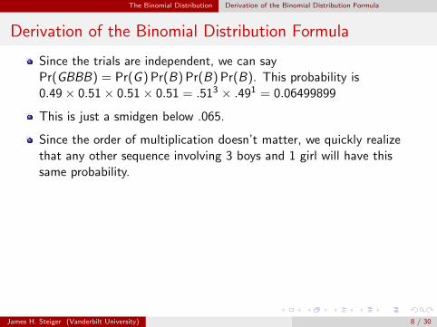
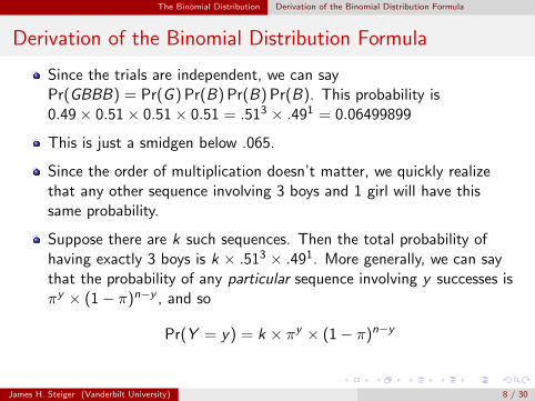
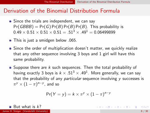
Since the trials are independent, we can sayPr(GBBB) = Pr(G ) Pr(B) Pr(B) Pr(B). This probability is0.49× 0.51× 0.51× 0.51 = .513 × .491 = 0.06499899
This is just a smidgen below .065.
Since the order of multiplication doesn’t matter, we quickly realizethat any other sequence involving 3 boys and 1 girl will have thissame probability.
Suppose there are k such sequences. Then the total probability ofhaving exactly 3 boys is k × .513 × .491. More generally, we can saythat the probability of any particular sequence involving y successes isπy × (1− π)n−y , and so
Pr(Y = y) = k × πy × (1− π)n−y
But what is k?
James H. Steiger (Vanderbilt University) 8 / 30
The Binomial Distribution Derivation of the Binomial Distribution Formula
Derivation of the Binomial Distribution Formula
Since the trials are independent, we can sayPr(GBBB) = Pr(G ) Pr(B) Pr(B) Pr(B). This probability is0.49× 0.51× 0.51× 0.51 = .513 × .491 = 0.06499899
This is just a smidgen below .065.
Since the order of multiplication doesn’t matter, we quickly realizethat any other sequence involving 3 boys and 1 girl will have thissame probability.
Suppose there are k such sequences. Then the total probability ofhaving exactly 3 boys is k × .513 × .491. More generally, we can saythat the probability of any particular sequence involving y successes isπy × (1− π)n−y , and so
Pr(Y = y) = k × πy × (1− π)n−y
But what is k?James H. Steiger (Vanderbilt University) 8 / 30
The Binomial Distribution Derivation of the Binomial Distribution Formula
Derivation of the Binomial Distribution FormulaCombinations
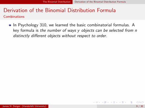
In Psychology 310, we learned the basic combinatorial formulas. Akey formula is the number of ways y objects can be selected from ndistinctly different objects without respect to order.
For example, you have the 4 letters A,B,C,D. How many different setsof size 2 may be selected from these 4 letters?
This is called “the number of combinations of 4 objects taken 2 at atime,” or “4 choose 2.”
James H. Steiger (Vanderbilt University) 9 / 30
The Binomial Distribution Derivation of the Binomial Distribution Formula
Derivation of the Binomial Distribution FormulaCombinations
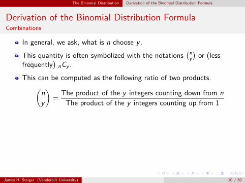
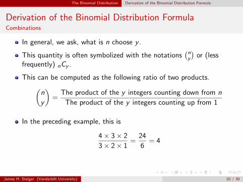
In general, we ask, what is n choose y .
This quantity is often symbolized with the notations(ny
)or (less
frequently) nCy .
This can be computed as the following ratio of two products.(n
y
)=
The product of the y integers counting down from n
The product of the y integers counting up from 1
In the preceding example, this is
4× 3× 2
3× 2× 1=
24
6= 4
James H. Steiger (Vanderbilt University) 10 / 30
The Binomial Distribution Derivation of the Binomial Distribution Formula
Derivation of the Binomial Distribution FormulaCombinations
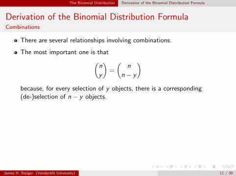
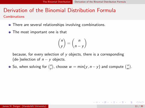
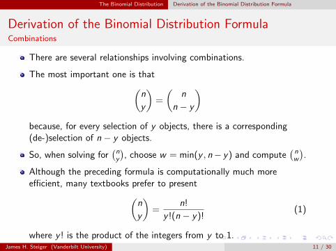
There are several relationships involving combinations.
The most important one is that(n
y
)=
(n
n − y
)because, for every selection of y objects, there is a corresponding(de-)selection of n − y objects.
So, when solving for(ny
), choose w = min(y , n− y) and compute
(nw
).
Although the preceding formula is computationally much moreefficient, many textbooks prefer to present(
n
y
)=
n!
y !(n − y)!(1)
where y ! is the product of the integers from y to 1.
James H. Steiger (Vanderbilt University) 11 / 30
The Binomial Distribution Derivation of the Binomial Distribution Formula
Derivation of the Binomial Distribution FormulaCombinations
There are several relationships involving combinations.
The most important one is that(n
y
)=
(n
n − y
)because, for every selection of y objects, there is a corresponding(de-)selection of n − y objects.
So, when solving for(ny
), choose w = min(y , n− y) and compute
(nw
).
Although the preceding formula is computationally much moreefficient, many textbooks prefer to present(
n
y
)=
n!
y !(n − y)!(1)
where y ! is the product of the integers from y to 1.James H. Steiger (Vanderbilt University) 11 / 30
The Binomial Distribution Derivation of the Binomial Distribution Formula
Derivation of the Binomial Distribution FormulaCombinations
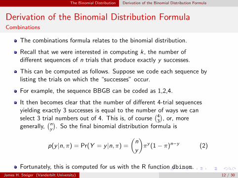
The combinations formula relates to the binomial distribution.
Recall that we were interested in computing k, the number ofdifferent sequences of n trials that produce exactly y successes.
This can be computed as follows. Suppose we code each sequence bylisting the trials on which the “successes” occur.
For example, the sequence BBGB can be coded as 1,2,4.
It then becomes clear that the number of different 4-trial sequencesyielding exactly 3 successes is equal to the number of ways we canselect 3 trial numbers out of 4. This is, of course
(43
), or, more
generally,(ny
). So the final binomial distribution formula is
p(y |n, π) = Pr(Y = y |n, π) =
(n
y
)πy (1− π)n−y (2)
Fortunately, this is computed for us with the R function dbinom.James H. Steiger (Vanderbilt University) 12 / 30
The Binomial Distribution The Binomial Distribution as a Sampling Distribution
The Binomial Distribution as a Sampling Distribution
The binomial distribution gives probabilities for the number ofsuccesses in n binomial trials.
However, since each number of successes yi corresponds to exactlyone sample proportion of successes yi/n,we see that we also havederived, in effect, the distribution of the sample proportion p.
For example, we previously determined that the probability of exactly3 boys out of 4 is roughly 0.26, and this implies that the probabilityof a proportion of 3/4 = .75 is also 0.26.
James H. Steiger (Vanderbilt University) 13 / 30
Hypothesis Testing
Hypothesis TestingParameters, Statistics, Estimators, and Spaces
A parameter, loosely speaking, as a numerical characteristic of astatistical population.
A statistic is any function of the sample.
An estimator of a parameter is a statistic that is used to approximatethe parameter from sample data. The observed value of an estimatoris an estimate of the parameter.
The parameter space is the set of all possible values of the parameter.
The sample space is the set of all possible values of the statisticemployed as an estimator of the parameter.
James H. Steiger (Vanderbilt University) 14 / 30
Hypothesis Testing
Hypothesis TestingNull and Alternative Hypotheses
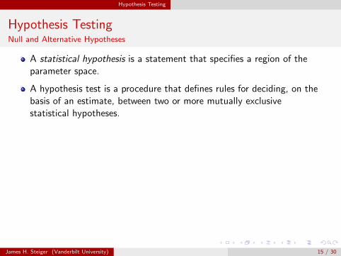
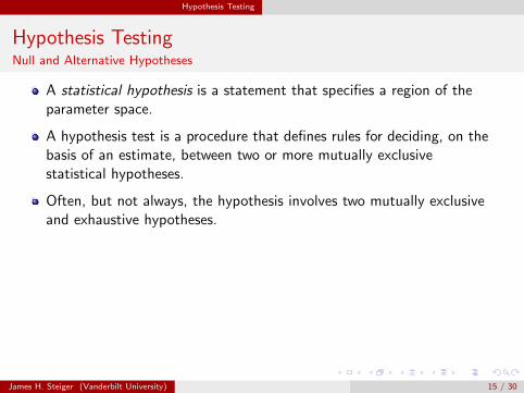
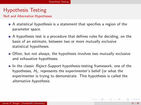
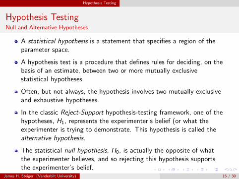
A statistical hypothesis is a statement that specifies a region of theparameter space.
A hypothesis test is a procedure that defines rules for deciding, on thebasis of an estimate, between two or more mutually exclusivestatistical hypotheses.
Often, but not always, the hypothesis involves two mutually exclusiveand exhaustive hypotheses.
In the classic Reject-Support hypothesis-testing framework, one of thehypotheses, H1, represents the experimenter’s belief (or what theexperimenter is trying to demonstrate. This hypothesis is called thealternative hypothesis.
The statistical null hypothesis, H0, is actually the opposite of whatthe experimenter believes, and so rejecting this hypothesis supportsthe experimenter’s belief.
James H. Steiger (Vanderbilt University) 15 / 30
Hypothesis Testing
Hypothesis TestingNull and Alternative Hypotheses
A statistical hypothesis is a statement that specifies a region of theparameter space.
A hypothesis test is a procedure that defines rules for deciding, on thebasis of an estimate, between two or more mutually exclusivestatistical hypotheses.
Often, but not always, the hypothesis involves two mutually exclusiveand exhaustive hypotheses.
In the classic Reject-Support hypothesis-testing framework, one of thehypotheses, H1, represents the experimenter’s belief (or what theexperimenter is trying to demonstrate. This hypothesis is called thealternative hypothesis.
The statistical null hypothesis, H0, is actually the opposite of whatthe experimenter believes, and so rejecting this hypothesis supportsthe experimenter’s belief.
James H. Steiger (Vanderbilt University) 15 / 30
Hypothesis Testing
Hypothesis TestingAn Example
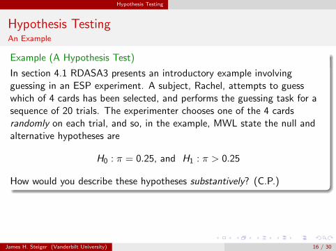
Example (A Hypothesis Test)
In section 4.1 RDASA3 presents an introductory example involvingguessing in an ESP experiment. A subject, Rachel, attempts to guesswhich of 4 cards has been selected, and performs the guessing task for asequence of 20 trials. The experimenter chooses one of the 4 cardsrandomly on each trial, and so, in the example, MWL state the null andalternative hypotheses are
H0 : π = 0.25, and H1 : π > 0.25
How would you describe these hypotheses substantively? (C.P.)
James H. Steiger (Vanderbilt University) 16 / 30
Hypothesis Testing
Hypothesis TestingAn Example
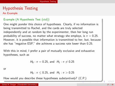
Example (A Hypothesis Test (ctd))
One might ponder this choice of hypotheses. Clearly, if no information isbeing transmitted to Rachel, and the cards are truly selectedindependently and at random by the experimenter, then her long runprobability of success, no matter what strategy she employs, is π = 0.25.However, it is possible that information is transmitted to her, but, becauseshe has “negative ESP,” she achieves a success rate lower than 0.25.
With this in mind, I prefer a pair of mutually exclusive and exhaustivehypotheses, such as
H0 : π = 0.25, and H1 : π 6= 0.25
orH0 : π ≤ 0.25, and H1 : π > 0.25
How would you describe these hypotheses substantively? (C.P.)
James H. Steiger (Vanderbilt University) 17 / 30
Hypothesis Testing
Hypothesis TestingThe Critical Region Approach
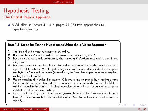
MWL discuss (boxes 4.1–4.2, pages 75–76) two approaches tohypothesis testing.
One approach is the p-value approach, described in Box 4.1.
James H. Steiger (Vanderbilt University) 18 / 30
Hypothesis Testing
Hypothesis TestingThe Critical Region Approach
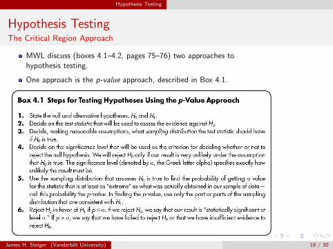
MWL discuss (boxes 4.1–4.2, pages 75–76) two approaches tohypothesis testing.
One approach is the p-value approach, described in Box 4.1.
James H. Steiger (Vanderbilt University) 18 / 30
Hypothesis Testing
Hypothesis TestingThe p-Value Approach
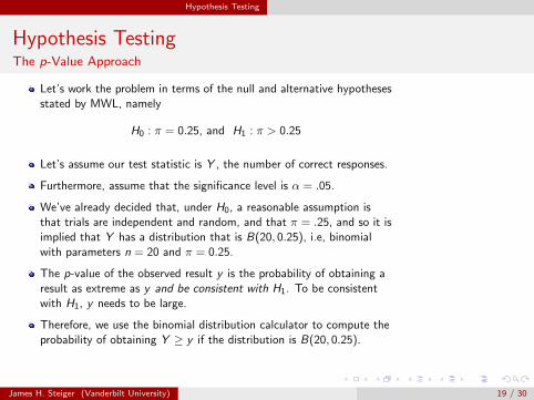
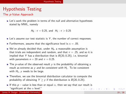
Let’s work the problem in terms of the null and alternative hypothesesstated by MWL, namely
H0 : π = 0.25, and H1 : π > 0.25
Let’s assume our test statistic is Y , the number of correct responses.
Furthermore, assume that the significance level is α = .05.
We’ve already decided that, under H0, a reasonable assumption isthat trials are independent and random, and that π = .25, and so it isimplied that Y has a distribution that is B(20, 0.25), i.e, binomialwith parameters n = 20 and π = 0.25.
The p-value of the observed result y is the probability of obtaining aresult as extreme as y and be consistent with H1. To be consistentwith H1, y needs to be large.
Therefore, we use the binomial distribution calculator to compute theprobability of obtaining Y ≥ y if the distribution is B(20, 0.25).
If this p − value is less than or equal α, then we say that our result is“significant at the α level.”
James H. Steiger (Vanderbilt University) 19 / 30

Hypothesis Testing
Hypothesis TestingThe p-Value Approach
Let’s work the problem in terms of the null and alternative hypothesesstated by MWL, namely
H0 : π = 0.25, and H1 : π > 0.25
Let’s assume our test statistic is Y , the number of correct responses.
Furthermore, assume that the significance level is α = .05.
We’ve already decided that, under H0, a reasonable assumption isthat trials are independent and random, and that π = .25, and so it isimplied that Y has a distribution that is B(20, 0.25), i.e, binomialwith parameters n = 20 and π = 0.25.
The p-value of the observed result y is the probability of obtaining aresult as extreme as y and be consistent with H1. To be consistentwith H1, y needs to be large.
Therefore, we use the binomial distribution calculator to compute theprobability of obtaining Y ≥ y if the distribution is B(20, 0.25).
If this p − value is less than or equal α, then we say that our result is“significant at the α level.”
James H. Steiger (Vanderbilt University) 19 / 30
Hypothesis Testing
Hypothesis TestingThe p-Value Approach
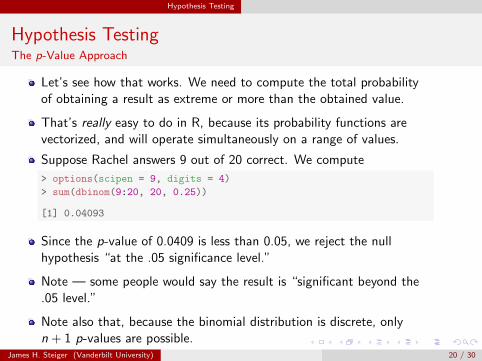
Let’s see how that works. We need to compute the total probabilityof obtaining a result as extreme or more than the obtained value.
That’s really easy to do in R, because its probability functions arevectorized, and will operate simultaneously on a range of values.
Suppose Rachel answers 9 out of 20 correct. We compute
> options(scipen = 9, digits = 4)
> sum(dbinom(9:20, 20, 0.25))
[1] 0.04093
Since the p-value of 0.0409 is less than 0.05, we reject the nullhypothesis “at the .05 significance level.”
Note — some people would say the result is “significant beyond the.05 level.”
Note also that, because the binomial distribution is discrete, onlyn + 1 p-values are possible.
James H. Steiger (Vanderbilt University) 20 / 30
Hypothesis Testing
Hypothesis TestingThe Critical (Rejection) Region Approach
With the Critical Region approach, we specify, in advance, whichvalues of the test statistic will cause us to reject the statistical nullhypothesis.
To have a “significance level” (α) of 0.05, we must control theprobability of incorrectly rejecting a true H0 at or below .05.
When the test statistic distribution is discrete, it is usually impossibleto control the probability of an incorrect rejection at exactly 0.05.
James H. Steiger (Vanderbilt University) 21 / 30
Hypothesis Testing
Hypothesis TestingThe Critical (Rejection) Region Approach
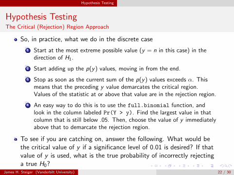
So, in practice, what we do in the discrete case
1 Start at the most extreme possible value (y = n in this case) in thedirection of H1.
2 Start adding up the p(y) values, moving in from the end.
3 Stop as soon as the current sum of the p(y) values exceeds α. Thismeans that the preceding y value demarcates the critical region.Values of the statistic at or above that value are in the rejection region.
4 An easy way to do this is to use the full.binomial function, andlook in the column labeled Pr(Y > y). Find the largest value in thatcolumn that is still below .05. Then, choose the value of y immediatelyabove that to demarcate the rejection region.
To see if you are catching on, answer the following. What would bethe critical value of y if a significance level of 0.01 is desired? If thatvalue of y is used, what is the true probability of incorrectly rejectinga true H0?
James H. Steiger (Vanderbilt University) 22 / 30
Hypothesis Testing
Hypothesis TestingNull and Alternative Hypotheses
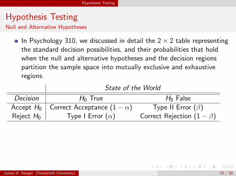
In Psychology 310, we discussed in detail the 2× 2 table representingthe standard decision possibilities, and their probabilities that holdwhen the null and alternative hypotheses and the decision regionspartition the sample space into mutually exclusive and exhaustiveregions.
State of the World
Decision H0 True H0 False
Accept H0 Correct Acceptance (1− α) Type II Error (β)Reject H0 Type I Error (α) Correct Rejection (1− β)
James H. Steiger (Vanderbilt University) 23 / 30
One-Tailed vs. Two-Tailed Tests
One-Tailed vs. Two-Tailed Tests
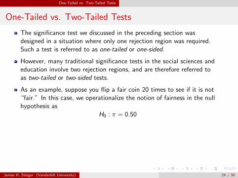
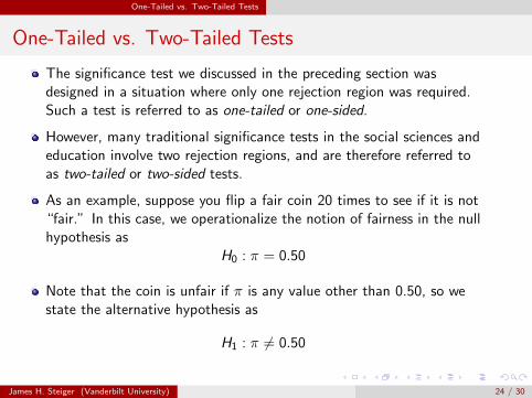
The significance test we discussed in the preceding section wasdesigned in a situation where only one rejection region was required.Such a test is referred to as one-tailed or one-sided.
However, many traditional significance tests in the social sciences andeducation involve two rejection regions, and are therefore referred toas two-tailed or two-sided tests.
As an example, suppose you flip a fair coin 20 times to see if it is not“fair.” In this case, we operationalize the notion of fairness in the nullhypothesis as
H0 : π = 0.50
Note that the coin is unfair if π is any value other than 0.50, so westate the alternative hypothesis as
H1 : π 6= 0.50
James H. Steiger (Vanderbilt University) 24 / 30
One-Tailed vs. Two-Tailed Tests
One-Tailed vs. Two-Tailed Tests
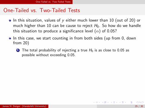
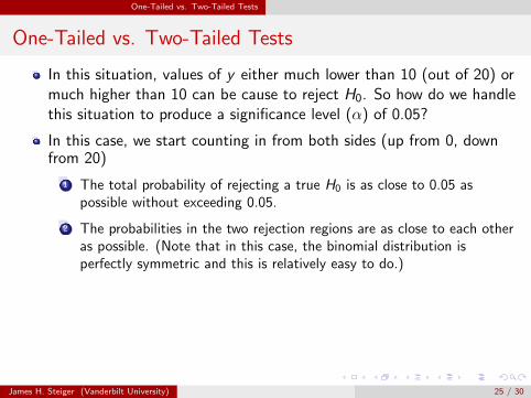
In this situation, values of y either much lower than 10 (out of 20) ormuch higher than 10 can be cause to reject H0. So how do we handlethis situation to produce a significance level (α) of 0.05?
In this case, we start counting in from both sides (up from 0, downfrom 20)
1 The total probability of rejecting a true H0 is as close to 0.05 aspossible without exceeding 0.05.
2 The probabilities in the two rejection regions are as close to each otheras possible. (Note that in this case, the binomial distribution isperfectly symmetric and this is relatively easy to do.)
James H. Steiger (Vanderbilt University) 25 / 30
One-Tailed vs. Two-Tailed Tests
One-Tailed vs. Two-Tailed Tests
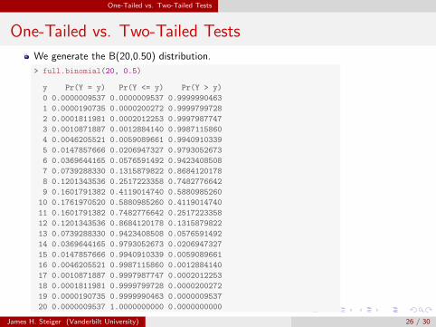
We generate the B(20,0.50) distribution.
> full.binomial(20, 0.5)
y Pr(Y = y) Pr(Y <= y) Pr(Y > y)
0 0.0000009537 0.0000009537 0.9999990463
1 0.0000190735 0.0000200272 0.9999799728
2 0.0001811981 0.0002012253 0.9997987747
3 0.0010871887 0.0012884140 0.9987115860
4 0.0046205521 0.0059089661 0.9940910339
5 0.0147857666 0.0206947327 0.9793052673
6 0.0369644165 0.0576591492 0.9423408508
7 0.0739288330 0.1315879822 0.8684120178
8 0.1201343536 0.2517223358 0.7482776642
9 0.1601791382 0.4119014740 0.5880985260
10 0.1761970520 0.5880985260 0.4119014740
11 0.1601791382 0.7482776642 0.2517223358
12 0.1201343536 0.8684120178 0.1315879822
13 0.0739288330 0.9423408508 0.0576591492
14 0.0369644165 0.9793052673 0.0206947327
15 0.0147857666 0.9940910339 0.0059089661
16 0.0046205521 0.9987115860 0.0012884140
17 0.0010871887 0.9997987747 0.0002012253
18 0.0001811981 0.9999799728 0.0000200272
19 0.0000190735 0.9999990463 0.0000009537
20 0.0000009537 1.0000000000 0.0000000000
James H. Steiger (Vanderbilt University) 26 / 30
One-Tailed vs. Two-Tailed Tests
One-Tailed vs. Two-Tailed Tests
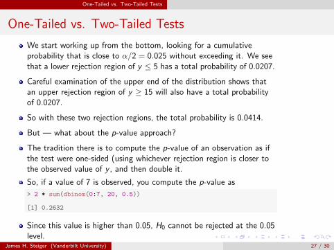
We start working up from the bottom, looking for a cumulativeprobability that is close to α/2 = 0.025 without exceeding it. We seethat a lower rejection region of y ≤ 5 has a total probability of 0.0207.
Careful examination of the upper end of the distribution shows thatan upper rejection region of y ≥ 15 will also have a total probabilityof 0.0207.
So with these two rejection regions, the total probability is 0.0414.
But — what about the p-value approach?
The tradition there is to compute the p-value of an observation as ifthe test were one-sided (using whichever rejection region is closer tothe observed value of y , and then double it.
So, if a value of 7 is observed, you compute the p-value as
> 2 * sum(dbinom(0:7, 20, 0.5))
[1] 0.2632
Since this value is higher than 0.05, H0 cannot be rejected at the 0.05level.
James H. Steiger (Vanderbilt University) 27 / 30
A General Approach to Power Calculation
The Power of a Statistical Test
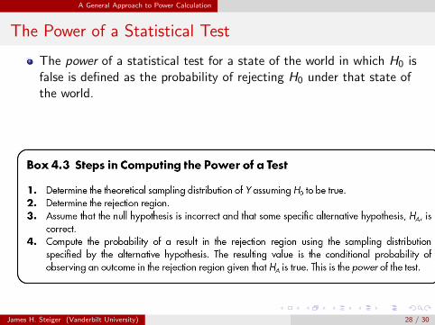
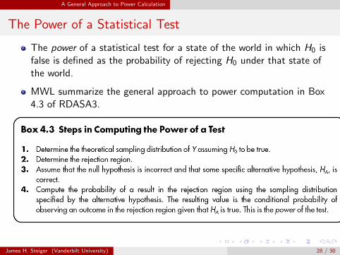
The power of a statistical test for a state of the world in which H0 isfalse is defined as the probability of rejecting H0 under that state ofthe world.
MWL summarize the general approach to power computation in Box4.3 of RDASA3.
James H. Steiger (Vanderbilt University) 28 / 30
A General Approach to Power Calculation
The Power of a Statistical Test
The power of a statistical test for a state of the world in which H0 isfalse is defined as the probability of rejecting H0 under that state ofthe world.
MWL summarize the general approach to power computation in Box4.3 of RDASA3.
James H. Steiger (Vanderbilt University) 28 / 30
A General Approach to Power Calculation
Power CalculationAn Example
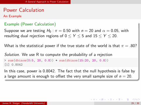
Example (Power Calculation)
Suppose we are testing H0 : π = 0.50 with n = 20 and α = 0.05, withresulting dual rejection regions of 0 ≤ Y ≤ 5 and 15 ≤ Y ≤ 20.
What is the statistical power if the true state of the world is that π = .80?
Solution. We use R to compute the probability of a rejection
> sum(dbinom(0:5, 20, 0.8)) + sum(dbinom(15:20, 20, 0.8))
[1] 0.8042
In this case, power is 0.8042. The fact that the null hypothesis is false bya large amount is enough to offset the very small sample size of n = 20.
James H. Steiger (Vanderbilt University) 29 / 30
A General Approach to Power Calculation Factors Affecting Power: A General Perspective
Factors Affecting PowerA General Perspective
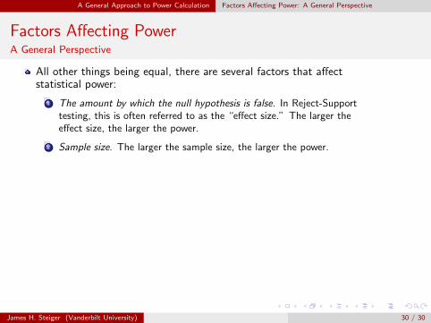
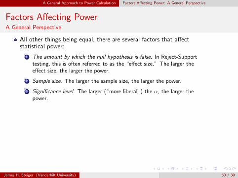
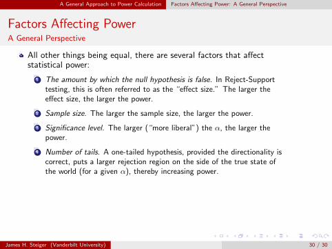
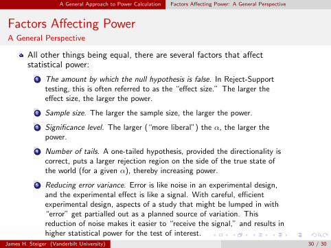
All other things being equal, there are several factors that affectstatistical power:
1 The amount by which the null hypothesis is false. In Reject-Supporttesting, this is often referred to as the “effect size.” The larger theeffect size, the larger the power.
2 Sample size. The larger the sample size, the larger the power.
3 Significance level. The larger (“more liberal”) the α, the larger thepower.
4 Number of tails. A one-tailed hypothesis, provided the directionality iscorrect, puts a larger rejection region on the side of the true state ofthe world (for a given α), thereby increasing power.
5 Reducing error variance. Error is like noise in an experimental design,and the experimental effect is like a signal. With careful, efficientexperimental design, aspects of a study that might be lumped in with“error” get partialled out as a planned source of variation. Thisreduction of noise makes it easier to “receive the signal,” and results inhigher statistical power for the test of interest.
James H. Steiger (Vanderbilt University) 30 / 30

A General Approach to Power Calculation Factors Affecting Power: A General Perspective
Factors Affecting PowerA General Perspective
All other things being equal, there are several factors that affectstatistical power:
1 The amount by which the null hypothesis is false. In Reject-Supporttesting, this is often referred to as the “effect size.” The larger theeffect size, the larger the power.
2 Sample size. The larger the sample size, the larger the power.
3 Significance level. The larger (“more liberal”) the α, the larger thepower.
4 Number of tails. A one-tailed hypothesis, provided the directionality iscorrect, puts a larger rejection region on the side of the true state ofthe world (for a given α), thereby increasing power.
5 Reducing error variance. Error is like noise in an experimental design,and the experimental effect is like a signal. With careful, efficientexperimental design, aspects of a study that might be lumped in with“error” get partialled out as a planned source of variation. Thisreduction of noise makes it easier to “receive the signal,” and results inhigher statistical power for the test of interest.
James H. Steiger (Vanderbilt University) 30 / 30