Gabor Analysis of Auditory Midbrain Receptive Fields ...anqi/journal/escabi_neurophy_2003.pdfGabor Analysis of Auditory Midbrain Receptive Fields: Spectro-Temporal and Binaural Composition

90:456-476, 2003. First published Mar 26, 2003; doi:10.1152/jn.00851.2002 J NeurophysiolAnqi Qiu, Christoph E. Schreiner and Monty A. Escabí Fields: Spectro-Temporal and Binaural Composition Gabor Analysis of Auditory Midbrain Receptive

You might find this additional information useful...

52 articles, 25 of which you can access free at: This article cites http://jn.physiology.org/cgi/content/full/90/1/456#BIBL

5 other HighWire hosted articles: This article has been cited by

[PDF] [Full Text] [Abstract]

, December 17, 2003; 23 (37): 11489-11504. J. Neurosci.M. A. Escabi, L. M. Miller, H. L. Read and C. E. Schreiner

ColliculusNaturalistic Auditory Contrast Improves Spectrotemporal Coding in the Cat Inferior

[PDF] [Full Text] [Abstract], October 1, 2005; 94 (4): 2970-2975. J Neurophysiol

R. Narayan, A. Ergun and K. Sen Delayed Inhibition in Cortical Receptive Fields and the Discrimination of Complex Stimuli


, October 12, 2005; 25 (41): 9524-9534. J. Neurosci.M. A. Escabi, R. Nassiri, L. M. Miller, C. E. Schreiner and H. L. Read

Content, and Information ThroughputThe Contribution of Spike Threshold to Acoustic Feature Selectivity, Spike Information

[PDF] [Full Text] [Abstract], December 1, 2005; 94 (6): 4051-4067. J Neurophysiol

K. N. O'Connor, C. I. Petkov and M. L. Sutter Adaptive Stimulus Optimization for Auditory Cortical Neurons


, December 1, 2005; 94 (6): 4441-4454. J NeurophysiolE. D. Young and B. M. Calhoun

Nonlinear Modeling of Auditory-Nerve Rate Responses to Wideband Stimuli

including high-resolution figures, can be found at: Updated information and services http://jn.physiology.org/cgi/content/full/90/1/456

can be found at: Journal of Neurophysiologyabout Additional material and information http://www.the-aps.org/publications/jn

This information is current as of September 26, 2006 .

http://www.the-aps.org/.American Physiological Society. ISSN: 0022-3077, ESSN: 1522-1598. Visit our website at (monthly) by the American Physiological Society, 9650 Rockville Pike, Bethesda MD 20814-3991. Copyright © 2005 by the

publishes original articles on the function of the nervous system. It is published 12 times a yearJournal of Neurophysiology

on Septem

ber 26, 2006 jn.physiology.org

Dow

nloaded from

http://jn.physiology.org/cgi/content/full/90/1/456#BIBL

http://jn.physiology.org/cgi/content/abstract/94/6/4441

http://jn.physiology.org/cgi/content/full/94/6/4441

http://jn.physiology.org/cgi/reprint/94/6/4441




http://www.jneurosci.org/cgi/content/abstract/25/41/9524

http://www.jneurosci.org/cgi/content/full/25/41/9524

http://www.jneurosci.org/cgi/reprint/25/41/9524




http://www.jneurosci.org/cgi/content/abstract/23/37/11489

http://www.jneurosci.org/cgi/content/full/23/37/11489

http://www.jneurosci.org/cgi/reprint/23/37/11489


http://www.the-aps.org/publications/jn

http://www.the-aps.org/

http://jn.physiology.org

Gabor Analysis of Auditory Midbrain Receptive Fields: Spectro-Temporaland Binaural Composition

Anqi Qiu,1 Christoph E. Schreiner,3 and Monty A. Escabı1,2

1Biomedical Engineering Program and 2Department of Electrical and Computer Engineering, University of Connecticut, Storrs,Connecticut 06269-2157; and 3W. M. Keck Center for Integrative Neuroscience, University of California, San Francisco, California 94143

Submitted 25 September 2002; accepted in final form 3 March 2003

Qiu, Anqi, Christoph E. Schreiner, and Monty A. Escabı. Gaboranalysis of auditory midbrain receptive fields: spectro-temporaland binaural composition. J Neurophysiol 90: 456 – 476, 2003;10.1152/jn.00851.2002. The spectro-temporal receptive field (STRF)is a model representation of the excitatory and inhibitory integrationarea of auditory neurons. Recently it has been used to study spectraland temporal aspects of monaural integration in auditory centers. Herewe report the properties of monaural STRFs and the relationshipbetween ipsi- and contralateral inputs to neurons of the central nucleusof cat inferior colliculus (ICC) of cats. First, we use an optimalsingular-value decomposition method to approximate auditory STRFsas a sum of time-frequency separable Gabor functions. This procedureextracts nine physiologically meaningful parameters. The STRFs of�60% of collicular neurons are well described by a time-frequencyseparable Gabor STRF model, whereas the remaining neurons exhib-ited obliquely oriented or multiple excitatory/inhibitory subfields thatrequire a nonseparable Gabor fitting procedure. Parametric analysisreveals distinct spectro-temporal tradeoffs in receptive field size andmodulation filtering resolution. Comparisons between an identicalmodel used to study spatio-temporal integration areas of visual neu-rons further shows that auditory and visual STRFs share numerousstructural properties. We then use the Gabor STRF model to comparequantitatively receptive field properties of contra- and ipsilateral in-puts to the ICC. We show that most interaural STRF parameters arehighly correlated bilaterally. However, the spectral and temporalphases of ipsi- and contralateral STRFs often differ significantly. Thissuggests that activity originating from each ear share various spectro-temporal response properties such as their temporal delay, bandwidth,and center frequency but have shifted or interleaved patterns ofexcitation and inhibition. These differences in converging monauralreceptive fields expand binaural processing capacity beyond interauraltime and intensity aspects and may enable colliculus neurons to detectdisparities in the spectro-temporal composition of the binaural input.

I N T R O D U C T I O N

Auditory neurons are unique for their ability to processrapidly varying stimuli and track changes in the stimulusspectrum. Neurons in central auditory stations are highly sen-sitive to dynamic variations in the temporal, spectral, intensity,and aural composition of the sensory stimulus (Goldberg andBrown 1969; Irvine and Gago 1990; Krishna and Semple 2000;Kuwada et al. 1997; Langner and Schreiner 1988; Ramachan-dran et al. 1999; Rees and Møller 1983). Although numerousstudies have evaluated the response characteristics to structur-

ally simple stimuli, only a handful of studies have analyzed thejoint spectral, temporal, and/or binaural receptive field arrange-ments responsible for this response diversity (Depireux et al.2001; Miller et al. 2002; Sen et al. 2001).

Auditory receptive fields are typically derived with isolatedpure tones that are presented at varying frequencies and inten-sities or by measuring neural sensitivity to narrowband time-varying stimuli (e.g., Krishna and Semple 2000; Langner andSchreiner 1988; Ramachandran et al. 1999; Rees and Møller1983). Recently, the auditory spectro-temporal receptive field(STRF), a linear model representation of the integration area ofa neuron, has expanded these classical methods. The auditorySTRF has the advantage that it simultaneously describes spec-tral and temporal stimulus attributes that preferentially activatea neuron and can be used to identify the spectral arrangementand temporal dynamics of neural excitation and inhibition of aneuron during dynamic broadband stimulation (Aersten et al.1980; deCharms et al. 1998; Depireux 2001; Escabı and Schre-iner 2002; Klein et al. 2000; Miller et al. 2002; Nelken et al.1997; Sen et al. 2001; Theunissen et al. 2000). In particular, theSTRF technique is useful for predicting neuronal responsepatterns to complex auditory stimuli, including natural sounds(Aersten et al. 1980; Klein et al. 2000; Sen et al. 2001;Theunissen et al. 2000), and can accurately account for spatialselectivity profiles that contribute to sound localization(Schnupp et al. 2001).

In the visual system, the direct counterpart of the auditorySTRF is the spatio-temporal receptive field. Here the spectraldimension (which extends along the primary sensory epithe-lium receptor surface of the cochlea) is replaced by spatialdimensions along the retinal sensory epithelium (Cai et al.1997; DeAngelis et al. 1995; De Valois and Cottaris 1998;Shamma 2001). Visual neurophysiologists have used Gaborand Gamma functions as quantitative descriptors of visualSTRFs (Cai et al. 1997; DeAngelis et al. 1993a, 1999; Jonesand Palmer 1987a,b). Advantages for fitting visual STRFs byquantitative functions include: improved estimates of the spa-tio-temporal structure of visual response areas and the removalof estimation noise. Furthermore, these model STRFs can beused to study the arrangements of excitatory and inhibitoryneural inputs and to extract physiologically meaningful param-eters from neural data (DeAngelis et al. 1993a, 1999). Al-

*Address for reprint requests: M. A. Escabı, University of Connecticut,Electrical and Computer Engineering Dept., 317 Fairfield Rd, Unit 1157,Storrs, CT 06269-2157 (E-mail: [email protected]).

The costs of publication of this article were defrayed in part by the paymentof page charges. The article must therefore be hereby marked ‘‘advertisement’’in accordance with 18 U.S.C. Section 1734 solely to indicate this fact.

J Neurophysiol 90: 456–476, 2003;10.1152/jn.00851.2002.

456 0022-3077/03 $5.00 Copyright © 2003 The American Physiological Society www.jn.org

on Septem


Dow

nloaded from


though it has been suggested that auditory and visual STRFshave remarkably similar time-varying structure (deCharms etal. 1998; Shamma 2001), only a few studies have quantitativelyevaluated the spectro-temporal structure of auditory STRFs(Depireux et al. 2001; Escabı and Schreiner 2002; Miller et al.2002; Sen et al. 2001). However, these studies did not quan-titatively compare the structure of the auditory STRF directlywith their visual counterpart.

In this study, we present a time-frequency Gabor STRFmodel to fit auditory STRFs in the central nucleus of cat’sinferior colliculus (ICC). Spectral and temporal Gabor func-tions are used to model spectral receptive field (SRF) andtemporal receptive field (TRF) profiles of ICC neurons, respec-tively. Each STRF is then fitted by a weighted sum of productsof time-frequency separable Gabor functions. From the defini-tion of a Gabor function, nine physiologically meaningfulparameters are extracted: the center frequency, the best rippledensity, the best temporal modulation frequency, the peaklatency, the bandwidth of the SRF profile, the response dura-tion, the response strength, and the spectral and temporalphases. These parameters are used to quantify spectral, tem-poral, and time-frequency response characteristics to dynamicmoving ripple stimuli (Escabı and Schreiner 2002; Miller et al.2002). This Gabor STRF model is a direct extension of recep-tive field models used to study the structure of visual receptivefields in the primary visual cortex (DeAngelis et al. 1993a,b,1999) and provides a basis for comparing the structure ofauditory and visual STRFs. In particular, we apply this meth-odology to compare STRF properties of contra- and ipsilateralinputs to ICC neurons. We demonstrate specific aural STRFdifferences that suggest binaural filtering mechanisms beyondintra-aural time and level sensitivity.

M A T E R I A L S A N D M E T H O D S

Electrophysiology

Physiological recording methods have been presented in detailelsewhere (Escabı and Schreiner 2002). Briefly, cats (n � 4) wereinitially anesthetized with a mixture of ketamine HCl (10 mg/kg) andacepromazine (0.28 mg/kg im). A surgical state of anesthesia wasinduced with �30 mg/kg pentobarbital sodium (Nembutal) and main-tained throughout the surgery with supplements via an intravenousinfusion line. Body temperature was measured and maintained at�37.5°C. The overlying cerebrum and part of the bony tentorium wasremoved to expose the ICC via a dorsal approach. During the unitrecordings, animals were maintained in an areflexive state via contin-uous infusion of ketamine (2–4 mg � kg�1 � h�1) and diazepam (0.4–1mg � kg�1 � h�1) in lactated Ringer solution (1–4 mg � kg�1 � h�1).The infusion rate was adjusted according to physiologic criteria (heartrate, breathing rate, temperature, and peripheral reflexes). All surgicalmethods and experiment procedures follow National Institutes ofHealth and U.S. Department of Agriculture guidelines.

Neural data was acquired from n � 99 single units in the ICC withparylen-coated tungsten microelectrodes (Microprobe, Potomac, MD;1–3 M� at 1 kHz) that were advanced into the central nucleus with ahydraulic microdrive (David Kopft Instruments, Tujunga, CA). Ac-tion potential traces were recorded onto a digital audio tape (CygnusTechnologies CDAT16; Delaware Water Gap, PA) at a sampling rateof 24.0 kHz (41.7-�s resolution) and spike sorted off-line with aBayesian spike sorting algorithm (Lewicki 1994).

Acoustic stimuli

Dynamic moving ripple (DMR) stimuli (Escabı and Schreiner2002) were presented with the animal in a sound-shielded chamber(IAC, Bronx, NY) with stimuli delivered via a closed, binauralspeaker system (electrostatic diaphragms from Stax). The DynamicMoving Ripple sound is specifically designed to dynamically activatethe primary sensory epithelium and to probe the physiologicallyrelevant range of spectral and temporal stimulus modulations ofneurons in an unbiased fashion. Sounds were presented binaurallywith an independent sound sequence to each ear—from which inde-pendent contra- and ipsi-lateral STRFs were computed via spike-triggered averaging (Escabı and Schreiner 2002).

In three experiments, the DMR stimulus was presented for a periodof 10–20 min (Escabı and Schreiner, 2002). In one experiment, atwo-repeat 4-min sequence of the DMR (8 min total) was presented.In all experiments, stimuli covered the same range of spectral andtemporal parameters and were presented at �30–70 dB above theneurons response threshold.

Gabor STRF model

STRFs were decomposed into a superposition of time-frequencyseparable functions from which we could model and fit each compo-nent by a spectro-temporal Gabor function (product of Gaussian andcosine; Fig. 3). Measured STRFs were first decomposed using asingular value decomposition (SVD) (Depireux et al. 2001; Press et al.1995; Theunissen et al. 2000) into a sum of separable STRF compo-nents (STRFi)

STRF�t, x� � U � S � V* � �i

STRFi�t, x�

S � diag��1, �2, · · ·�i, · · ·�, �1 � �2 � · · ·�i � · · · � 0 (1)

where U and V are unitary orthogonal matrixes containing the tem-poral and spectral receptive field profiles of each STRF component(Fig. 3, B and C; top and right); S is a diagonal matrix with real,non-negative elements, �i, in descending rank order according toenergy; and * denotes the Hermitian transpose. Each STRF compo-nent, STRFi, is obtained by the vector product

STRFi�t, x� � �i � ui � v*i (2)

where �i is the ith singular value of STRF(t, x) and determines theenergy of the ith STRF component. ui and vi are the ith unitaryorthogonal vectors of U and V, respectively. Conceptually, thesecorrespond to the spectral and temporal receptive field profiles of eachcomponent STRF (e.g., shown on the top and right of Fig. 3, B and C).The dominant spectral and temporal receptive field profiles, u1 and v1,account for �80% of the total STRF energy, and we therefore usethese to quantify spectral and temporal response characteristicsthroughout.

According to the SVD procedure, every STRFi component is time-frequency separable (although the entire STRF may be nonseparable).Therefore each component can be modeled by the product of aspectral and a temporal waveform, which we approximate by a Gaborfunction. Thus the fitted STRF model is expressed as a weighted sumof a finite set of N of statistically significant separable Gabor compo-nents (typically, N � 1 or 2)

STRFm�t, x� � �i�1

N

STRFim�t, x� � �i�1

N

sign � Ki � Gi�x� � Hi�t� (3)

where STRFm(t, x) (e.g., in Fig. 3F) is the fitted STRF model.STRFim(t, x) (e.g., in Fig. 3, D and E) is the fitted STRFi component.Ki, Gi(x), and Hi(t) correspond to the response strength, the fitted andnormalized SRF profile, and the fitted and normalized TRF profile ofthe ith STRF component, STRFi. The modeled spectral and temporalprofiles, Gi(x) and Hi(t), assume the form of a Gabor function (see

457GABOR ANALYSIS OF AUDITORY RECEPTIVE FIELDS

J Neurophysiol • VOL 90 • JULY 2003 • www.jn.org

on Septem


Dow

nloaded from


Eqs. 11 and 13, respectively) each with an independent set of spectraland temporal parameters. Finally, the variable sign assumes a value of1 or �1 and is included in the model to designate the type of STRF,which can be dominantly excitatory (�) or inhibitory (�), respec-tively. The optimal parameters of the Gabor-STRF model are deter-mined iteratively by minimizing the mean square error between themodel and the real data (Press et al. 1995).

Level of noise

Auditory STRFs are estimated from real neural data by a spike-triggered average method (Escabı and Schreiner 2002) that is inher-ently noisy. Measurement noise corresponds to random deviationsfrom the expected STRF that would result from an infinite amount ofaveraging. These variations result from unexpected variations in theneural response and from finite data averaging due to the finiteexperiment recording periods (Klein et al. 2000; Theunissen 2000).Therefore to minimize the effects of noise, it is necessary to consideronly those independent time-frequency components of the GaborSTRF model that significantly contribute to the STRF’s energy andstructure.

To determine the maximum number of independent dimensions ofthe STRF that contribute to its structure (N in Eq. 3), it is essential toquantify the STRF noise level. Singular values that exceed the mea-sured noise level typically contribute significantly to the neural re-sponse and should therefore be incorporated into the Gabor STRFmodel; alternately, singular values that fall below the noise levelcontribute largely to the noise and can therefore be ignored. Asignificant noise level (P � 0.01) was determined empirically via abootstrap STRF re-estimation procedure for a random Poisson firingneuron of identical spike rate as the neuron under investigation.Twenty-five randomly constructed STRFs, STRFr (e.g., Fig. 4A),were simulated by correlating a random Poisson spike train of firingrate, �, with the dynamic moving ripple noise stimulus. The firstsingular value (�r1) of each random-STRF, STRFr, was obtaineddirectly by performing a SVD. For each of the 25 trials (shown byvertical red circles in Fig. 4B), the measured level of noise wasrandomly distributed. Therefore the desired threshold noise level fora specific spike rate (solid line in Fig. 4B) was determined as the sumof the mean of �r1 and 2.57 times its SD (P � 0.01). The mean SDof �r1 were calculated from the 25 simulated samples by a bootstrapresampling technique (Efron and Tibshirani 1993). All first-orderSTRFs considered here were above the estimated noise level.

Similarity index

The Gabor STRF model can potentially account for much of thestructure of collicular receptive fields, however, the utility of themodel needs to be quantitatively evaluated. We devised three metricsto validate the goodness of fit of the model. We evaluated thegoodness of fit of SRF and TRF profiles independently and for theentire STRF.

To compare the receptive field structure of the model and data, wedevised the spectral similarity index (SIs), temporal similarity index(SIt) and spectro-temporal similarity index (SI). The spectral SI, SIs,accounts for differences in shape between original and model SRFprofiles; SIt is used to compare the original and model TRF profiles;the spectro-temporal SI, SI, measures shape differences between orig-inal and model STRFs. Individually these metrics correspond to acorrelation analysis performed between the model and original data(DeAngelis et al. 1999; Escabı and Schreiner 2002; Miller et al. 2002)and can be expressed as

SIs �SRF, SRFm�

�SRF� � �SRFm�(4)

SIt �TRF, TRFm�

�TRF� � �TRFm�(5)

SI �STRF, STRFm�

�STRF� � �STRFm�(6)

where ,� corresponds to the vector correlation, and � � � designates thevector norm operator. Because the STRF is formally defined by atwo-dimensional matrix of spectral and temporal samples, Eq. 6 couldnot be evaluated directly since it requires vector inputs. Therefore thestatistically significant samples of the STRF that exceeded a signifi-cance criterion of P � 0.002, were converted into a unidimensionalvector, from which the SI was determined using Eq. 6 (Escabı andSchreiner 2002).

Because all three similarity indices are effectively correlation co-efficients between the real data and model waveforms, they assume avalue of one whenever the waveforms inside their arguments areidentical in shape, zero if the waveforms have nothing in common andnegative one if the waveforms have identical shapes but differ by anegative sign.

Normalized mean square error

A fourth metric was defined that quantifies the relative difference inenergy between the fitted (STRFm) and the measured STRF (STRF).The normalized mean square error (MSE) is defined as the energy ofthe difference STRF normalized by the energy of a measured STRF(DeAngelis et al. 1999)

MSE �

¥s

¥t

�STRFm � STRF�2

¥s

¥t

STRF2 (7)

The MSE assumes values between zero and one, where lower MSEvalues are indicative of a properly fitted STRF.

Temporal asymmetry index

Initial evaluation of the temporal receptive field envelope revealedthat timing profiles of ICC neurons are characterized by sharp tran-sient onset. We therefore quantitatively evaluated the structure of thetemporal response envelope. To evaluate the degree of temporalasymmetry in the TRF profile, we define an asymmetry index (�t) asthe skewness of the temporal envelope (Bliss 1967)

�t �� t � �t�

3 � Et�t� � dt

� �t � �t�2 � Et�t� � dt�3/2 (8)

where �t is the mean or centroid of the temporal envelope, Et(t),measured at the center frequency (x0) of the neuron and normalizedfor unit area. A temporal asymmetry index of zero is observed only forTRF envelopes with perfectly symmetric envelopes about the meanpoint, �t. A �t significantly less than 0 indicates that the TRF profileis skewed to the right; and a �t significantly greater than 0 indicatesthe TRF profile is skewed to the left.

Separability index

An inherent aspect of the Gabor model is that it is composed ofmultiple receptive field components, each of which is a time-fre-quency separable function. If the receptive field contains only onesingular value, the receptive field is time-frequency separable; that is,it can be described by a multiplicative product of a temporal andspectral receptive field profile as in Eq. 2. Hypothetically, such aneuron would encode spectral and temporal information indepen-dently. If, alternately, the receptive field has multiple significantsingular values, the receptive field will exhibit time-frequency insep-arable structure. This can manifest as obliquely oriented STRF fea-tures or multiple asymmetrically aligned excitatory and inhibitoryreceptive field subregions. Neurons with such receptive field arrange-ments most likely prefer sound stimuli with dynamically changing

458 A. QIU, C. E. SCHREINER, AND M. A. ESCABI


on Septem


Dow

nloaded from


frequency components, and, consequently, the spectral and temporaldimensions for such neurons cannot be treated independently of eachother. This effect becomes more pronounced if the higher-order sin-gular values account for a large proportion of the receptive fieldenergy. Thus we can define a separability index by considering theproportion of energy provided by first singular value in relationship tothe cumulative energy of the higher-order singular values. We definethe separability index (�d) as

�d �

�12 � ¥

i�2

N

�i2

�12 ¥

i�2

N

�i2

(9)

where �1 and �i are the first- and higher-order singular values of theSTRF (Eq. 1), and N is the number of statistically significant singularvalues used in the Gabor STRF model. Conceptually, �d is defined asthe normalized energy of the first singular value (relative to the totalenergy of the model STRF) minus the normalized energy of thehigher-order singular values. Separability index values range from 0to 1; where 1 corresponds to a perfectly separable STRF and valuesclose to zero designate a highly inseparable receptive field arrange-ment.

R E S U L T S

We studied in 99 single neurons how dynamic stimuli areencoded in the ICC by identifying structural characteristics ofthe auditory STRF. Our dynamic moving ripple stimulus(DMR) is a broadband sound that efficiently probes spectro-temporal attributes of the acoustic space (Escabı and Schreiner2002). It is characterized by a dynamically changing spectrumwith widespread spectral fluctuations over a broad range ofresolutions (0–4 cycles/octave). Superimposed on this spectralvariability, the DMR exhibits temporal energy fluctuationsover a wide range of modulation frequencies: 0–350 Hz. Itsstatistically unbiased properties makes the stimulus directlyapplicable for the study of auditory receptive fields duringdynamic stimulation. We combined STRF measurement tech-niques with a spectro-temporal Gabor model to study thestructural properties and binaural arrangements of inferior col-liculus STRFs. This model allows us to extract nine physio-logically meaningful STRF parameters. To determine whetherthe Gabor model is well suited for describing auditory STRFs,we first fitted each contralateral STRF to the Gabor model andfound the optimal parameters of each receptive field. Next, weindependently characterized spectral and temporal receptivefield profiles as well as the arrangement of excitation andinhibition of each neuron in order to determine how thesedimensions contribute to the STRF. Finally, we use the GaborSTRF model to characterize and compare ipsi- and contralat-eral receptive field arrangements. By studying the spectral andtemporal parameters of the contralateral and ipsilateral STRFs,we identify how the spectro-temporal arrangement of excita-tion and inhibition contribute to the formation of binauralresponse properties seen in the inferior colliculus.

Structure of the spectral receptive field

The spectral receptive field (SRF) profile is a model repre-sentation of the frequency integration area of auditory neurons(Calhoun and Schreiner 1998; Kowalski et al. 1996; Miller etal. 2002; Schreiner and Calhoun 1994; Versnell and Shamma1998). This descriptor can be used to quantify neuronal re-

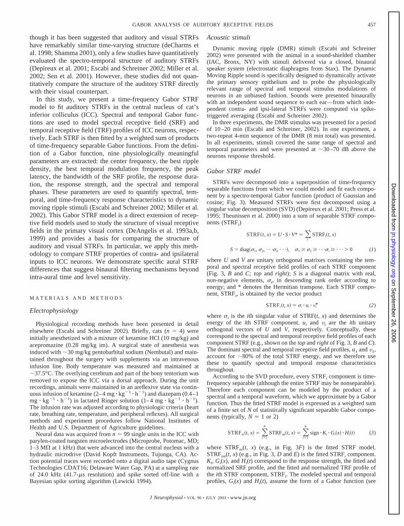
sponses to sounds with complex spectra (such as for formanttransitions in speech and spectral resonances in animal vocal-izations) and to study the receptive field arrangement of exci-tation and inhibition along the cochleotopic dimension of thestimulus. Most studies using this descriptor largely focused onqualitatively identifying general integration properties (such asthe arrangement of spectral excitation and inhibition) and onlyfor stimuli with static temporal characteristics. By slicing theSTRF at a fixed latency (solid lines in Fig. 1, B and C) we canstudy the dynamic behavior of the SRF profile for complexstimuli with time-varying structure. Specifically, we would liketo identify a model representation of the STRF that quantita-tively captures the general characteristics of the SRF profileand its associated dynamics. When the latency is �40 ms, thereis no discernible SRF structure for the STRF shown in Fig. 1A.At shorter latencies, however, SRF profiles can exhibit pureexcitation, inhibition, or an alternating arrangement of excita-tion and inhibition. The phase of SRF profiles changes contin-uously so that the excitatory bandwidths and center frequencieschange with increasing latency. Consequently, there is nodirect analytic equation to model the SRF profile at all laten-cies.

One step toward solving this problem is to break up the SRFprofile into an envelope and a carrier component via the Hilberttransform (Cai et al. 1997; Daugman 1985; DeAngelis et al.1993a, 1999; Jones and Palmer 1987a,b; Marcelja 1980). Theenvelope, Es(x), is computed by the vector sum of the SRFprofile, SRF(x), and its Hilbert transform, H[SRF(x)]

Es�x� � �SRF�x�2 H SRF�x��2 (10)

Example spectral envelopes of a single neuron are shown asdashed lines at two latencies in Fig. 1, B and C. The Hilberttransforms of each envelope, H[SRF(x)] (Fig. 1, B and C), arerepresented by the dotted lines and are obtained by shifting thephase of all frequency components of SRF(x) by 90° (solidlines in Fig. 1, B and C). Conceptually, the Hilbert transformisolates the fine carrier structure from the coarse envelopestructure of the STRF.

Although the SRF profile depends strongly on the latency ofthe STRF, the spectral envelope assumes a nearly invariantstructure at all latencies. The envelopes of the SRF profiles(dashed lines in Fig. 1, B and C) are approximately Gaussianfunctions and can be conveniently defined by their bandwidthand center frequency. The bandwidth of the SRF profile isdefined as the width of the envelope at a response level that is1/e relative to the absolute maximum of the envelope, captur-ing �85% of the energy in a Gaussian the SRF envelope. Thecenter frequency is defined as the peak value of the spectralenvelope. As expected for the SRF profiles of Fig. 1, B and C,the measured bandwidths and center frequencies along theexcitatory and inhibitory cross-sections are in close agreement:bandwidth � 1.00 and 0.89 octaves (octave is defined as log2(f/fr), fr � 500 Hz is a reference frequency), respectively;center frequency � 4.37 and 4.42 octaves.

The spectral receptive field structure was modeled at eachtime point as the product of a Gaussian envelope and a sinu-soidal carrier. Qualitatively, the Gaussian function defines thecenter and extent over which the neuron integrates spectralinformation, whereas the sinusoid carrier component is neces-sary to account for the interleaved patterns of excitation andinhibition. This functional form of the SRF profile, a Gabor



on Septem


Dow

nloaded from


function, is a direct extension of the receptive field modelsused to study spatio-temporal integration in the visual system(Cai et al. 1997; Daugman 1985; DeAngelis et al. 1993a; Jonesand Palmer 1987a,b; Marcelja 1980). The Gabor function cancapture numerous receptive field aspects and can be used toextract physiologically meaningful parameters directly fromthe neuron’s receptive field.

At each time point, the SRF profile was fitted by a Gaborfunction taking the general form

G�x� � K � e� 2�x�x0�/BW�2cos 2 � �0 � �x � x0� P� (11)

where K, x0, BW, �0, and P are free parameters. The parameterK models the strength of the spectral response in unit of spikes �s�1 � dB�1. x0 is the center frequency or the central position ofthe SRF envelope in units of octaves; BW is the bandwidth ofthe SRF which accounts for the spectral extent of the receptivefield; �0 is the best ripple density (units of cycles/octaves) thatmodels the distance between the excitatory and inhibitorylobes; P is the spectral phase of the SRF profile with respect tothe center frequency of the Gaussian envelope. This parameteraccounts for the alignment of excitation and inhibition relativeto the peak of the SRF envelope. The optimal parameters in Eq.11 can be obtained by minimizing the mean square errorbetween the Gabor function and the measured SRF profile(Press et al. 1995). Example SRF profiles (Fig. 1, D and E) andoptimal-fitted results are shown in Fig. 1, D and E at twolatencies of the STRF. Fitted profiles (continuous red lines) andthe measured SRF profiles (continuous black lines) are in closeagreement.

Structure of the temporal receptive field

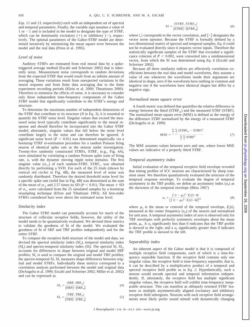
The structure of the temporal receptive field (TRF) profilewas analyzed using a similar functional descriptor as for theSRF profile. The TRF profile obtained by slicing through theSTRF at a particular frequency has an alternating arrangementof excitation and inhibition. The TRF profiles of collicularneurons typically have short excitation (or inhibition) followedby long inhibition (or excitation) (e.g., solid line in Fig. 2B),and their envelopes are, therefore, not symmetric about thepeak point. For example, the envelope of the TRF profileshown by the dashed line in Fig. 2B is not symmetric about thepeak of the temporal envelope (vertical line) because it has a

sharp onset and slower off-response. Because of this temporalasymmetry, the TRF profile is not well described by a sym-metric Gabor function.

The degree of temporal asymmetry was measured for allcontralateral responsive neurons in our ICC sample (n � 93 of99) with an asymmetry index, �t (see METHODS). The TRFprofile in Fig. 2B is skewed to the left and it therefore has apositive asymmetry index (0.935). Figure 2C (blue histogram)illustrates the distribution of asymmetry indices, obtained forthe dynamic moving ripple sound. The population distributionshows a bias toward positive values (mean SD: 1.93 1.64;

A B

C

D

E

FIG. 1. Spectral receptive field (SRF) profile analysis. A typical inferior colliculus spectro-temporal receptive field (STRF) showingobliquely oriented excitatory and inhibitory subregions (A). Two SRF profiles taken along the excitatory (T � 12.7 ms) and inhibitory(T � 26.7 ms) spectral cross-sections (solid lines in B and C, respectively). Their Hilbert transform (H[SRF(x)]) are represented by dottedlines and their spectral envelope, Es(x), by dashed-lines (B and C). The neuron’s center frequency (CF) is determined from the peak ofthe SRF envelope. Typically, the CF is close to the peak of the SRF profile (as in B), although these may differ depending on thearrangement of spectral excitation and inhibition (as in C). The bandwidth of the SRF profile, BW, is measured directly from the spectralenvelope. The range of frequencies covered by the BW account for �85% of the energy of the SRF envelope. Measured SRF profile (redline) and Gabor fitted SRF profile (black line) are typically in close agreement (D and E).

FIG. 2. Asymmetry analysis of the temporal receptive field (TRF) profiles.A: typical STRF showing a short excitatory onset response and a long inhib-itory offset response. The TRF profile is obtained by taking a temporalcross-section about the center frequency (x0) (solid line in B) and its envelopeis extracted with the Hilbert transform (dashed line in B). The envelope showsa strong asymmetry about its peak point, which is designated by the verticalline. C: the distribution of asymmetry index (�s) for our sample of neurons isdisplaced toward positive values (blue histogram). After performing a time-warping transformation, temporal envelopes are nearly symmetric and theasymmetry indices are tightly distributed about 0 (red histogram). D: the TRFprofile of A (black line) was fitted with a skewed Gabor function (red line)which takes into account the temporal asymmetry of the TRF profile.



on Septem


Dow

nloaded from


observed range: 0.30–9.7; t-test, P � 0.001), indicating thatthe temporal envelopes and TRF profiles are skewed towardzero delay. Accordingly, the temporal responses profiles ofmost ICC neurons exhibit a short primary response (excitatoryor inhibitory) followed by a long secondary response of oppo-site sign (inhibitory or excitatory, respectively). Such timingdifferences between the onset and offset of the receptive fieldare consistent with asymmetric preferences to ramped auditorystimuli observed both physiologically (Lu et al. 2001) andpsychoacoustically (Neuhoff 1998; Patterson 1994).

Considering the observed temporal asymmetry, we modifiedthe Gabor model so that it accounts for the observed timingprofiles by incorporating a time-warping factor that skews thetime axis and allows us to model the TRF with a symmetricGabor function (DeAngelis et al. 1999). The time-skewingfunction was defined as

T � 2 � arctan �� t� (12)

where � is the skewing factor (observed range: 0.45–0.68), t isthe uncompressed time-axis, and T is the corrected temporalaxis. The TRF profile is then fitted by a Gabor function of theform

H�t� � K � e� 2�T�T0�/D�2� cos 2 � Fm0

� �T � T0� Q� (13)

where K, T0, D, Fm0, and Q are free parameters. K corresponds

to the strength of the temporal response; T0 is the peak latencyof the TRF profile; D reflects the time-skewed duration of theresponse; the best temporal modulation frequency is describedby Fm0

; and Q is the phase of a sinusoid component about T0.During the fitting procedure, each parameter was adjustediteratively until the optimal parameters in Eqs. 12 and 13 arefound by minimizing the mean square error between the modeland the measured TRF profile (Press et al. 1995). An examplefitted TRF profiles is illustrated in Fig. 2D. The fitted TRFprofile (solid red line) captures the structure of the measuredTRF profile (solid black line). Further analysis of the entirepopulation confirms the validity of the temporal receptive fieldasymmetry and the appropriateness of the time-skewing pa-rameter. We recomputed the asymmetry index of all neuronsusing the time-warped TRF profiles (Fig. 2C; red histogram),which resemble symmetric Gaussian functions (not shown).The time-warped asymmetry indices were near zero (time-warped mean SE � 0.083 0.014) and were significantlysmaller than for the unwarped TRF (time-unwarped, 1.93 0.17; paired t-test, P � 1). Thus the time-warping factoraccurately accounts for the observed temporal receptive fieldasymmetry observed for all ICC neurons.

Gabor-STRF model

The analysis of the TRF and SRF profiles shows that thetemporal and spectral receptive field dimensions of auditoryneurons can in principle be independently approximated bytemporal and spectral Gabor functions. Does this approachgeneralize for the STRF? Can we model the auditory STRF bya product of Gabor TRF and SRF profiles? If so, what condi-tions must be satisfied?

In terms of time and frequency response interactions, audi-tory STRFs can be divided into two fundamental types: sepa-rable and inseparable (Adelson and Bergen 1985; DeAngelis etal. 1995; Depireux et al. 2001; Miller et al. 2002; Reid et al.

1991; Sen et al. 2001). Time-frequency separability of theSTRF occurs whenever the STRF can be described as theproduct of a SRF profile and a TRF profile, in which case theSRF and TRF profiles are independent of each other. If aseparable STRF is taken into the Fourier domain, the rippletransfer function (RTF) is symmetric about the zero temporalmodulation frequency axis (Depireux et al. 2001; Escabı andSchreiner 2002; Miller et al. 2002; Sen et al. 2001). However,inseparable STRFs cannot be broken down into two indepen-dent time and frequency functions. The representations of theseSTRFs in the Fourier domain can therefore show conspicuousasymmetries (Depireux et al. 2001; Escabı and Schreiner 2002;Miller et al. 2002; Sen et al. 2001).

Many auditory STRFs have some inseparable features, in-cluding, time-frequency oriented subregions or multiple asym-metrically aligned excitatory and inhibitory receptive fieldcomponents. Such structural features may be necessary toencode specific structural components in natural signals, suchas consonant-vowel transitions in speech, and to dynamicallytrack changes in the frequency spectrum of complex signals,such as frequency-modulated sweeps.

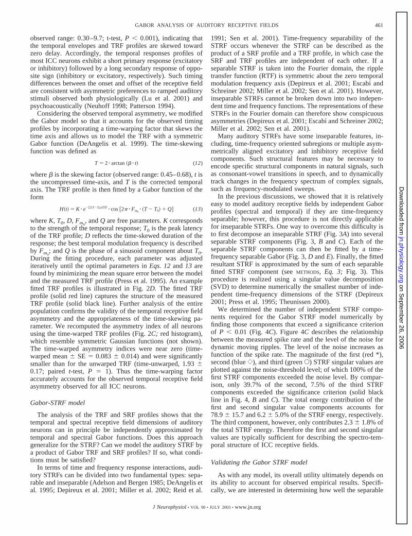
In the previous discussions, we showed that it is relativelyeasy to model auditory receptive fields by independent Gaborprofiles (spectral and temporal) if they are time-frequencyseparable; however, this procedure is not directly applicablefor inseparable STRFs. One way to overcome this difficulty isto first decompose an inseparable STRF (Fig. 3A) into severalseparable STRF components (Fig. 3, B and C). Each of theseparable STRF components can then be fitted by a time-frequency separable Gabor (Fig. 3, D and E). Finally, the fittedresultant STRF is approximated by the sum of each separablefitted STRF component (see METHODS, Eq. 3; Fig. 3). Thisprocedure is realized using a singular value decomposition(SVD) to determine numerically the smallest number of inde-pendent time-frequency dimensions of the STRF (Depireux2001; Press et al. 1995; Theunissen 2000).

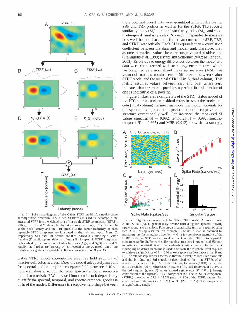
We determined the number of independent STRF compo-nents required for the Gabor STRF model numerically byfinding those components that exceed a significance criterionof P � 0.01 (Fig. 4C). Figure 4C describes the relationshipbetween the measured spike rate and the level of the noise fordynamic moving ripples. The level of the noise increases asfunction of the spike rate. The magnitude of the first (red *),second (blue {), and third (green E) STRF singular values areplotted against the noise-threshold level; of which 100% of thefirst STRF components exceeded the noise level. By compar-ison, only 39.7% of the second, 7.5% of the third STRFcomponents exceeded the significance criterion (solid blackline in Fig. 4, B and C). The total energy contribution of thefirst and second singular value components accounts for78.9 15.7 and 6.2 5.0% of the STRF energy, respectively.The third component, however, only contributes 2.3 1.8% ofthe total STRF energy. Therefore the first and second singularvalues are typically sufficient for describing the spectro-tem-poral structure of ICC receptive fields.

Validating the Gabor STRF model

As with any model, its overall utility ultimately depends onits ability to account for observed empirical results. Specifi-cally, we are interested in determining how well the separable



on Septem


Dow

nloaded from


Gabor STRF model accounts for receptive field structure ofinferior colliculus neurons. Does the model adequately accountfor spectral and/or temporal receptive field structures? If so,how well does it account for joint spectro-temporal receptivefield characteristics? We devised four metrics to independentlyquantify the spectral, temporal, and spectro-temporal goodnessof fit of the model. Differences in receptive field shape between

the model and neural data were quantified individually for theSRF and TRF profiles as well as for the STRF. The spectralsimilarity index (SIs), temporal similarity index (SIt), and spec-tro-temporal similarity index (SI) each independently measurehow well the model accounts for the structure of the SRF, TRF,and STRF, respectively. Each SI is equivalent to a correlationcoefficient between the data and model, and, therefore, theyassume numerical values between negative and positive one(DeAngelis et al. 1999; Escabı and Schreiner 2002; Miller et al.2002). Errors due to energy differences between the model anddata were characterized with an energy error metric—whichwe computed as a normalized mean square error (MSE; seeMETHODS) from the residual errors (difference between GaborSTRF model and the original STRF; Fig. 5, third column). Thismetric assumes values between zero and one, where zeroindicates that the model provides a perfect fit and a value ofone is indicative of a poor fit.

Figure 5 illustrates example fits of the STRF Gabor model offive ICC neurons and the residual errors between the model anddata (third column). In most instances, the model accounts forthe spectral, temporal, and spectro-temporal receptive fieldstructure exceptionally well. For instance, the measured SIvalues (spectral SI � 0.992; temporal SI � 0.992; spectro-temporal SI � 0.967) and MSE (0.043) show that a strongly

FIG. 3. Schematic diagram of the Gabor STRF model. A singular valuedecomposition procedure (SVD; see METHODS) is used to decompose themeasured STRF into a weighted sum of separable STRF components (STRF1,STRF2, . . . ; B and C; shown for the 1st 2 components only). The SRF profileat the peak latency and the TRF profile at the center frequency of eachseparable STRF component are illustrated on the right and top of B and C,respectively. SRF and TRF profiles are then individually fitted by a Gaborfunction (D and E; top and right waveforms). Each separable STRF componentis described by the product of 2 Gabor functions [Gi(x) and Hi(t)] in D and E.Finally, the fitted STRF (STRFm, F) is modeled as the weighted sum of thestatistically significant separable STRF components (from D and E).

A B

C D

FIG. 4. Significance analysis of the Gabor STRF model. A random noiseSTRF, STRFr (A), is generated by reverse-correlating the dynamic movingripple sound and a random, Poisson-distributed spike train at a specific spikerate (� � 3.93 spikes/s for this example). The noise level is obtained bymeasuring the first singular value (�r1 � 0.42 for the shown example) of theSTRFr with the SVD method used to break up the STRF into separablecomponents (Fig. 3). For each spike rate this procedure is resimulated 25 timesto estimate the distribution of noise-levels (vertical red circles in B). Aresampling bootstrap technique is used to estimate the threshold-level requiredto achieve a significance of P � 0.01 at each spike rate (continuous line, B andC). The relationship between the noise-threshold level, the measured spike rateand the 1st, 2nd, and 3rd singular values obtained from the STRFs of allneurons is depicted in (C). All of the 1st-singular values (100%) exceed thenoise threshold (red *), whereas only 39.7% of the 2nd (blue {), and 7.5% ofthe 3rd singular (green E) values exceed significance (P � 0.01). Energycontribution of the separable STRF component (D). The 1st STRF component,(STRF1) accounts for 78.9 15.7% (mean SD) of the STRFs energy. Thecontributions of the 2nd (6.2 5.0%) and 3rd (2.3 1.8%) STRF componentsis significantly smaller.



on Septem


Dow

nloaded from


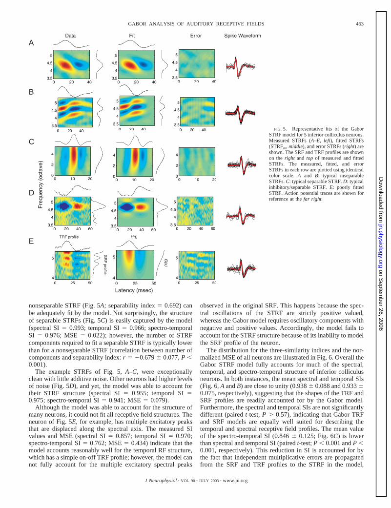
nonseparable STRF (Fig. 5A; separability index � 0.692) canbe adequately fit by the model. Not surprisingly, the structureof separable STRFs (Fig. 5C) is easily captured by the model(spectral SI � 0.993; temporal SI � 0.966; spectro-temporalSI � 0.976; MSE � 0.022); however, the number of STRFcomponents required to fit a separable STRF is typically lowerthan for a nonseparable STRF (correlation between number ofcomponents and separability index: r � �0.679 0.077, P �0.001).

The example STRFs of Fig. 5, A–C, were exceptionallyclean with little additive noise. Other neurons had higher levelsof noise (Fig. 5D), and yet, the model was able to account fortheir STRF structure (spectral SI � 0.955; temporal SI �0.975; spectro-temporal SI � 0.941; MSE � 0.079).

Although the model was able to account for the structure ofmany neurons, it could not fit all receptive field structures. Theneuron of Fig. 5E, for example, has multiple excitatory peaksthat are displaced along the spectral axis. The measured SIvalues and MSE (spectral SI � 0.857; temporal SI � 0.970;spectro-temporal SI � 0.762; MSE � 0.434) indicate that themodel accounts reasonably well for the temporal RF structure,which has a simple on-off TRF profile; however, the model cannot fully account for the multiple excitatory spectral peaks

observed in the original SRF. This happens because the spec-tral oscillations of the STRF are strictly positive valued,whereas the Gabor model requires oscillatory components withnegative and positive values. Accordingly, the model fails toaccount for the STRF structure because of its inability to modelthe SRF profile of the neuron.

The distribution for the three-similarity indices and the nor-malized MSE of all neurons are illustrated in Fig. 6. Overall theGabor STRF model fully accounts for much of the spectral,temporal, and spectro-temporal structure of inferior colliculusneurons. In both instances, the mean spectral and temporal SIs(Fig. 6, A and B) are close to unity (0.938 0.088 and 0.933 0.075, respectively), suggesting that the shapes of the TRF andSRF profiles are readily accounted for by the Gabor model.Furthermore, the spectral and temporal SIs are not significantlydifferent (paired t-test, P � 0.57), indicating that Gabor TRFand SRF models are equally well suited for describing thetemporal and spectral receptive field profiles. The mean valueof the spectro-temporal SI (0.846 0.125; Fig. 6C) is lowerthan spectral and temporal SI (paired t-test; P � 0.001 and P �0.001, respectively). This reduction in SI is accounted for bythe fact that independent multiplicative errors are propagatedfrom the SRF and TRF profiles to the STRF in the model,

C

A

D

E

B

FIG. 5. Representative fits of the GaborSTRF model for 5 inferior colliculus neurons.Measured STRFs (A–E, left), fitted STRFs(STRFm, middle), and error STRFs (right) areshown. The SRF and TRF profiles are shownon the right and top of measured and fittedSTRFs. The measured, fitted, and errorSTRFs in each row are plotted using identicalcolor scale. A and B: typical inseparableSTRFs. C: typical separable STRF. D: typicalinhibitory/separable STRF. E: poorly fittedSTRF. Action potential traces are shown forreference at the far right.



on Septem


Dow

nloaded from


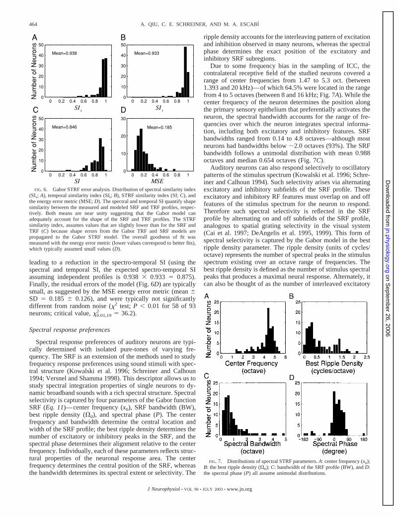
leading to a reduction in the spectro-temporal SI (using thespectral and temporal SI, the expected spectro-temporal SIassuming independent profiles is 0.938 � 0.933 � 0.875).Finally, the residual errors of the model (Fig. 6D) are typicallysmall, as suggested by the MSE energy error metric (mean SD � 0.185 0.126), and were typically not significantlydifferent from random noise (�2 test; P � 0.01 for 58 of 93neurons; critical value, �0.01,19

2 � 36.2).

Spectral response preferences

Spectral response preferences of auditory neurons are typi-cally determined with isolated pure-tones of varying fre-quency. The SRF is an extension of the methods used to studyfrequency response preferences using sound stimuli with spec-tral structure (Kowalski et al. 1996; Schreiner and Calhoun1994; Versnel and Shamma 1998). This descriptor allows us tostudy spectral integration properties of single neurons to dy-namic broadband sounds with a rich spectral structure. Spectralselectivity is captured by four parameters of the Gabor functionSRF (Eq. 11)—center frequency (x0), SRF bandwidth (BW),best ripple density (�0), and spectral phase (P). The centerfrequency and bandwidth determine the central location andwidth of the SRF profile; the best ripple density determines thenumber of excitatory or inhibitory peaks in the SRF, and thespectral phase determines their alignment relative to the centerfrequency. Individually, each of these parameters reflects struc-tural properties of the neuronal response area. The centerfrequency determines the central position of the SRF, whereasthe bandwidth determines its spectral extent or selectivity. The

ripple density accounts for the interleaving pattern of excitationand inhibition observed in many neurons, whereas the spectralphase determines the exact position of the excitatory andinhibitory SRF subregions.

Due to some frequency bias in the sampling of ICC, thecontralateral receptive field of the studied neurons covered arange of center frequencies from 1.47 to 5.3 oct. (between1.393 and 20 kHz)—of which 64.5% were located in the rangefrom 4 to 5 octaves (between 8 and 16 kHz; Fig. 7A). While thecenter frequency of the neuron determines the position alongthe primary sensory epithelium that preferentially activates theneuron, the spectral bandwidth accounts for the range of fre-quencies over which the neuron integrates spectral informa-tion, including both excitatory and inhibitory features. SRFbandwidths ranged from 0.14 to 4.8 octaves—although mostneurons had bandwidths below �2.0 octaves (93%). The SRFbandwidth follows a unimodal distribution with mean 0.988octaves and median 0.654 octaves (Fig. 7C).

Auditory neurons can also respond selectively to oscillatorypatterns of the stimulus spectrum (Kowalski et al. 1996; Schre-iner and Calhoun 1994). Such selectivity arises via alternatingexcitatory and inhibitory subfields of the SRF profile. Theseexcitatory and inhibitory RF features must overlap on and offfeatures of the stimulus spectrum for the neuron to respond.Therefore such spectral selectivity is reflected in the SRFprofile by alternating on and off subfields of the SRF profile,analogous to spatial grating selectivity in the visual system(Cai et al. 1997; DeAngelis et al. 1995, 1999). This form ofspectral selectivity is captured by the Gabor model in the bestripple density parameter. The ripple density (units of cycles/octave) represents the number of spectral peaks in the stimulusspectrum existing over an octave range of frequencies. Thebest ripple density is defined as the number of stimulus spectralpeaks that produces a maximal neural response. Alternately, itcan also be thought of as the number of interleaved excitatory

FIG. 6. Gabor STRF error analysis. Distribution of spectral similarity index(SIs; A), temporal similarity index (SIt; B), STRF similarity index (SI; C), andthe energy error metric (MSE; D). The spectral and temporal SI quantify shapesimilarity between the measured and modeled SRF and TRF profiles, respec-tively. Both means are near unity suggesting that the Gabor model canadequately account for the shape of the SRF and TRF profiles. The STRFsimilarity index, assumes values that are slightly lower than for the SRF andTRF (C) because shape errors from the Gabor TRF and SRF models arepropagated to the Gabor STRF model. The overall goodness of fit wasmeasured with the energy error metric (lower values correspond to better fits),which typically assumed small values (D).

FIG. 7. Distributions of spectral STRF parameters. A: center frequency (x0);B: the best ripple density (�0); C: bandwidth of the SRF profile (BW), and D:the spectral phase (P) all assume unimodal distributions.



on Septem


Dow

nloaded from


and inhibitory subunits of the SRF existing over a single octave(Escabı and Schreiner 2002; Klein et al. 2000; Miller et al.2002; Schreiner and Calhoun 1994). Most neurons in oursample preferred low ripple densities (Fig. 7B; mean � 0.609cycles/octave; median � 0.406 cycles/octave), indicating thatthey preferred broad spectral features of the dynamic movingripple sound. The range of best ripple densities extended fromnearly 0 (0.022 cycles/octave) to 2.113 cycles/octave althoughall neurons were tested up to 4 cycles/octave.

Finally, the spectral phase of the SRF profile determines thealignment of excitatory and inhibitory features relative to thecenter frequency of the neuron. Conceptually, a spectral phaseshift corresponds to a frequency shift of the actual SRF max-imum (not the envelope peak or center frequency). A positivephase value shifts the maximum of the spectral profile to lowerfrequencies; a negative phase shifts the SRF maximum tohigher frequencies. Most of the STRFs (78.5%) have positivespectral phases, indicating that neurons favor lower frequen-cies than the center frequency (Fig. 7D).

The SRF profile allows us to study its arrangement in termsof spectral excitation and inhibition. The behavior of eachneuron can also be interpreted directly in the ripple density orfrequency domain (Kowalski et al. 1996; Miller et al. 2002;Schreiner and Calhoun 1994). To do this, the SRF is convertedinto a spectral modulation transfer function (sMTF). The sMTFmeasures the neurons response (spikes � s�1 � dB�1) as afunction of the applied ripple density. Using the Gabor modelrepresentation of the SRF profile (Eq. 11), the correspondingsMTF is obtained by applying a Fourier transform magnitude(FTM) to the SRF profile

G�x� � K � e� 2�x�x0�/BW�2� cos 2 � �0 � �x � x0� P�s FTM

sMTF�� A � e� �BW��0�/2�2(14)

where all symbols are defined as in Eq. 11. The parameter A,determines the peak magnitude of the MTF or equivalently thegain of the neuron from stimulus to response (units spikes/s/dB). It is related to the magnitude of the SRF through therelationship: A � K � BW � �/4. The sMTF acquires thestructure of a Gaussian function with the center �0 and stan-dard deviation �2//BW. The bandwidth of the sMTF isdefined as the width of the sMTF that accounts for 85% of thetotal energy under the Gaussian curve. This parameter deter-mines the range of spectral oscillations (cycles/octave) in astimulus that can potentially activate the neuron. According tothis criterion, the tail points at the level of 1/e of the GaussiansMTF peak value delineate the bandwidth of the sMTF. Com-pared to the bandwidth of the SRF profile, the bandwidth of thesMTF (4//BW) is inversely proportional to the bandwidth ofthe SRF profile (BW).

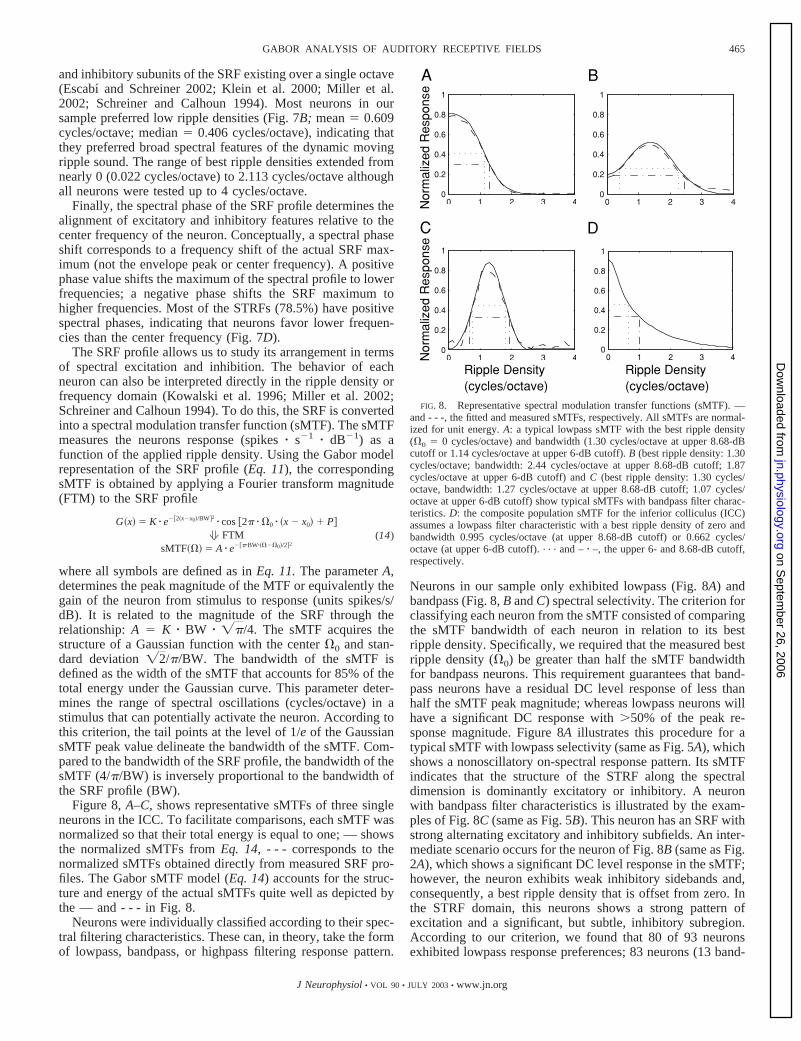
Figure 8, A–C, shows representative sMTFs of three singleneurons in the ICC. To facilitate comparisons, each sMTF wasnormalized so that their total energy is equal to one; — showsthe normalized sMTFs from Eq. 14, - - - corresponds to thenormalized sMTFs obtained directly from measured SRF pro-files. The Gabor sMTF model (Eq. 14) accounts for the struc-ture and energy of the actual sMTFs quite well as depicted bythe — and - - - in Fig. 8.

Neurons were individually classified according to their spec-tral filtering characteristics. These can, in theory, take the formof lowpass, bandpass, or highpass filtering response pattern.

Neurons in our sample only exhibited lowpass (Fig. 8A) andbandpass (Fig. 8, B and C) spectral selectivity. The criterion forclassifying each neuron from the sMTF consisted of comparingthe sMTF bandwidth of each neuron in relation to its bestripple density. Specifically, we required that the measured bestripple density (�0) be greater than half the sMTF bandwidthfor bandpass neurons. This requirement guarantees that band-pass neurons have a residual DC level response of less thanhalf the sMTF peak magnitude; whereas lowpass neurons willhave a significant DC response with �50% of the peak re-sponse magnitude. Figure 8A illustrates this procedure for atypical sMTF with lowpass selectivity (same as Fig. 5A), whichshows a nonoscillatory on-spectral response pattern. Its sMTFindicates that the structure of the STRF along the spectraldimension is dominantly excitatory or inhibitory. A neuronwith bandpass filter characteristics is illustrated by the exam-ples of Fig. 8C (same as Fig. 5B). This neuron has an SRF withstrong alternating excitatory and inhibitory subfields. An inter-mediate scenario occurs for the neuron of Fig. 8B (same as Fig.2A), which shows a significant DC level response in the sMTF;however, the neuron exhibits weak inhibitory sidebands and,consequently, a best ripple density that is offset from zero. Inthe STRF domain, this neurons shows a strong pattern ofexcitation and a significant, but subtle, inhibitory subregion.According to our criterion, we found that 80 of 93 neuronsexhibited lowpass response preferences; 83 neurons (13 band-

FIG. 8. Representative spectral modulation transfer functions (sMTF). —and - - -, the fitted and measured sMTFs, respectively. All sMTFs are normal-ized for unit energy. A: a typical lowpass sMTF with the best ripple density(�0 � 0 cycles/octave) and bandwidth (1.30 cycles/octave at upper 8.68-dBcutoff or 1.14 cycles/octave at upper 6-dB cutoff). B (best ripple density: 1.30cycles/octave; bandwidth: 2.44 cycles/octave at upper 8.68-dB cutoff; 1.87cycles/octave at upper 6-dB cutoff) and C (best ripple density: 1.30 cycles/octave, bandwidth: 1.27 cycles/octave at upper 8.68-dB cutoff; 1.07 cycles/octave at upper 6-dB cutoff) show typical sMTFs with bandpass filter charac-teristics. D: the composite population sMTF for the inferior colliculus (ICC)assumes a lowpass filter characteristic with a best ripple density of zero andbandwidth 0.995 cycles/octave (at upper 8.68-dB cutoff) or 0.662 cycles/octave (at upper 6-dB cutoff). . . . and – � –, the upper 6- and 8.68-dB cutoff,respectively.



on Septem


Dow

nloaded from


pass and 70 lowpass) had best ripple densities offset from zero(as for Fig. 8B) and 69 had best ripple densities �1 cycle/octave. Thirteen neurons exhibited bandpass selectivity, and noneurons had highpass response preferences.

Each individual sMTF tells us about the spectral selectivityof individual neurons and tells us little about the overall spec-tral filtering capabilities of the inferior colliculus. Therefore,we determined the overall spectral selectivity of the inferiorcolliculus by computing a population sMTF. The populationsMTF of the inferior colliculus (Fig. 8D) was obtained byaveraging the amplitude-normalized sMTFs of all single neu-rons. Using the criterion defined for single unit sMTFs, we findthat the spectral selectivity of the ICC (in the sampled fre-quency range) is lowpass with a bandwidth of 0.995 cycles/octave (at upper 8.68 dB cutoff; according to the 1/e bandwidthcriterion) or 0.662 cycles/octave (at upper 6 dB cutoff) andcentered about a best ripple density of zero cycles/octave. Thusthe ICC as a whole has a significant preference for broadbandstimuli.

Temporal response preferences

Neurons in the ICC show a diverse range of response pref-erences to temporally modulated stimuli (e.g., Krishna andSemple 2000; Langner and Schreiner 1988; Ramachandran etal. 1999; Rees and Møller 1983). While numerous studies haveidentified the output-response characteristics of ICC neurons tosimple time-varying stimuli, the receptive field structure lead-ing to these response preferences has previously not beenstudied. Temporal response characteristics of ICC neurons canbe interpreted by four parameters of the temporal Gabor model(Eq. 13)—the best temporal modulation frequency (Fm0

), thepeak latency (T0), the response duration (D), and the temporalphase (Q). Together, the peak latency and response durationdetermine the locality and width of the TRF profile, respec-tively; the best temporal modulation frequency and temporalphase determine the rate and alignment of the temporal oscil-lation of the TRF profile.

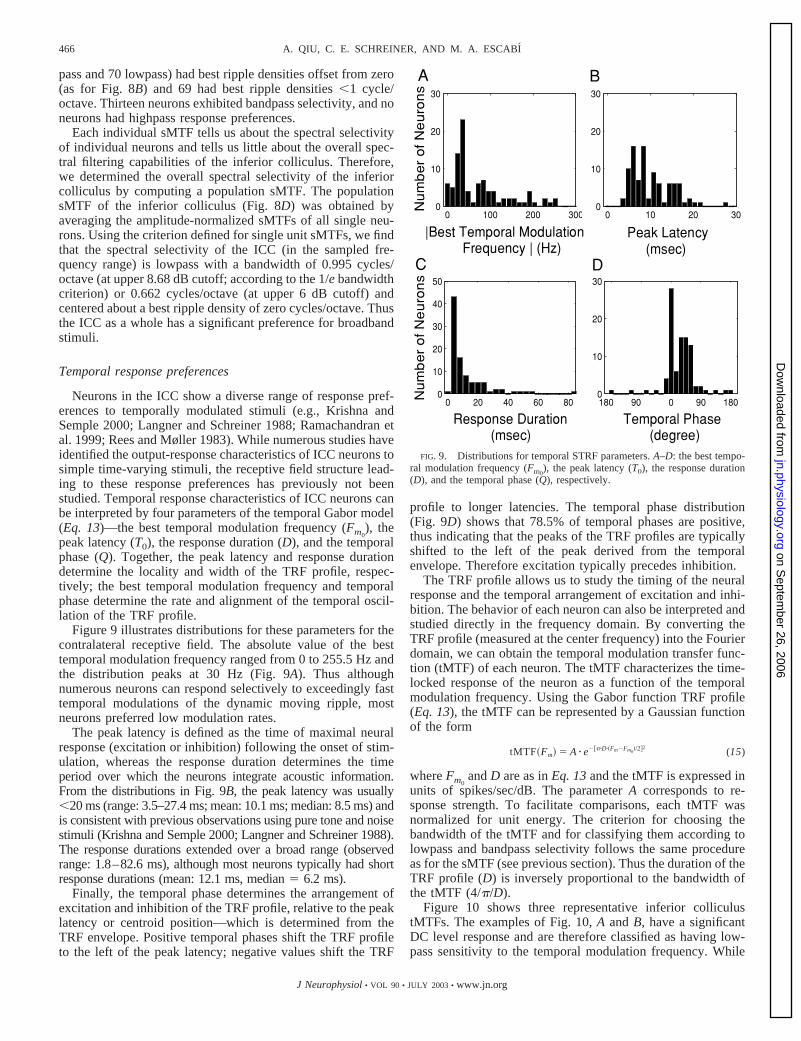
Figure 9 illustrates distributions for these parameters for thecontralateral receptive field. The absolute value of the besttemporal modulation frequency ranged from 0 to 255.5 Hz andthe distribution peaks at 30 Hz (Fig. 9A). Thus althoughnumerous neurons can respond selectively to exceedingly fasttemporal modulations of the dynamic moving ripple, mostneurons preferred low modulation rates.

The peak latency is defined as the time of maximal neuralresponse (excitation or inhibition) following the onset of stim-ulation, whereas the response duration determines the timeperiod over which the neurons integrate acoustic information.From the distributions in Fig. 9B, the peak latency was usually�20 ms (range: 3.5–27.4 ms; mean: 10.1 ms; median: 8.5 ms) andis consistent with previous observations using pure tone and noisestimuli (Krishna and Semple 2000; Langner and Schreiner 1988).The response durations extended over a broad range (observedrange: 1.8–82.6 ms), although most neurons typically had shortresponse durations (mean: 12.1 ms, median � 6.2 ms).

Finally, the temporal phase determines the arrangement ofexcitation and inhibition of the TRF profile, relative to the peaklatency or centroid position—which is determined from theTRF envelope. Positive temporal phases shift the TRF profileto the left of the peak latency; negative values shift the TRF

profile to longer latencies. The temporal phase distribution(Fig. 9D) shows that 78.5% of temporal phases are positive,thus indicating that the peaks of the TRF profiles are typicallyshifted to the left of the peak derived from the temporalenvelope. Therefore excitation typically precedes inhibition.

The TRF profile allows us to study the timing of the neuralresponse and the temporal arrangement of excitation and inhi-bition. The behavior of each neuron can also be interpreted andstudied directly in the frequency domain. By converting theTRF profile (measured at the center frequency) into the Fourierdomain, we can obtain the temporal modulation transfer func-tion (tMTF) of each neuron. The tMTF characterizes the time-locked response of the neuron as a function of the temporalmodulation frequency. Using the Gabor function TRF profile(Eq. 13), the tMTF can be represented by a Gaussian functionof the form

tMTF�Fm� � A � e� �D��Fm�Fm0�/2�2

(15)

where Fm0and D are as in Eq. 13 and the tMTF is expressed in

units of spikes/sec/dB. The parameter A corresponds to re-sponse strength. To facilitate comparisons, each tMTF wasnormalized for unit energy. The criterion for choosing thebandwidth of the tMTF and for classifying them according tolowpass and bandpass selectivity follows the same procedureas for the sMTF (see previous section). Thus the duration of theTRF profile (D) is inversely proportional to the bandwidth ofthe tMTF (4//D).

Figure 10 shows three representative inferior colliculustMTFs. The examples of Fig. 10, A and B, have a significantDC level response and are therefore classified as having low-pass sensitivity to the temporal modulation frequency. While

FIG. 9. Distributions for temporal STRF parameters. A–D: the best tempo-ral modulation frequency (Fm0

), the peak latency (T0), the response duration(D), and the temporal phase (Q), respectively.



on Septem


Dow

nloaded from


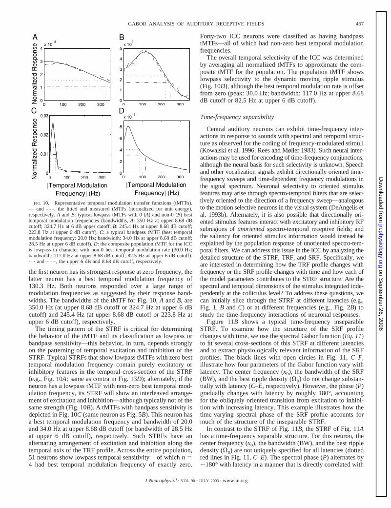
the first neuron has its strongest response at zero frequency, thelatter neuron has a best temporal modulation frequency of130.3 Hz. Both neurons responded over a large range ofmodulation frequencies as suggested by their response band-widths. The bandwidths of the tMTF for Fig. 10, A and B, are350.0 Hz (at upper 8.68 dB cutoff or 324.7 Hz at upper 6 dBcutoff) and 245.4 Hz (at upper 8.68 dB cutoff or 223.8 Hz atupper 6 dB cutoff), respectively.

The timing pattern of the STRF is critical for determiningthe behavior of the tMTF and its classification as lowpass orbandpass sensitivity—this behavior, in turn, depends stronglyon the patterning of temporal excitation and inhibition of theSTRF. Typical STRFs that show lowpass tMTFs with zero besttemporal modulation frequency contain purely excitatory orinhibitory features in the temporal cross-section of the STRF(e.g., Fig. 10A; same as contra in Fig. 13D); alternately, if theneuron has a lowpass tMTF with non-zero best temporal mod-ulation frequency, its STRF will show an interleaved arrange-ment of excitation and inhibition—although typically not of thesame strength (Fig. 10B). A tMTFs with bandpass sensitivity isdepicted in Fig. 10C (same neuron as Fig. 5B). This neuron hasa best temporal modulation frequency and bandwidth of 20.0and 34.0 Hz at upper 8.68 dB cutoff (or bandwidth of 28.5 Hzat upper 6 dB cutoff), respectively. Such STRFs have analternating arrangement of excitation and inhibition along thetemporal axis of the TRF profile. Across the entire population,51 neurons show lowpass temporal sensitivity—of which n �4 had best temporal modulation frequency of exactly zero.

Forty-two ICC neurons were classified as having bandpasstMTFs—all of which had non-zero best temporal modulationfrequencies.

The overall temporal selectivity of the ICC was determinedby averaging all normalized tMTFs to approximate the com-posite tMTF for the population. The population tMTF showslowpass selectivity to the dynamic moving ripple stimulus(Fig. 10D), although the best temporal modulation rate is offsetfrom zero (peak: 30.0 Hz; bandwidth: 117.0 Hz at upper 8.68dB cutoff or 82.5 Hz at upper 6 dB cutoff).

Time-frequency separability

Central auditory neurons can exhibit time-frequency inter-actions in response to sounds with spectral and temporal struc-ture as observed for the coding of frequency-modulated stimuli(Kowalski et al. 1996; Rees and Møller 1983). Such neural inter-actions may be used for encoding of time-frequency conjunctions,although the neural basis for such selectivity is unknown. Speechand other vocalization signals exhibit directionally oriented time-frequency sweeps and time-dependent frequency modulations inthe signal spectrum. Neuronal selectivity to oriented stimulusfeatures may arise through spectro-temporal filters that are selec-tively oriented to the direction of a frequency sweep—analogousto the motion selective neurons in the visual system (DeAngelis etal. 1993b). Alternately, it is also possible that directionally ori-ented stimulus features interact with excitatory and inhibitory RFsubregions of unoriented spectro-temporal receptive fields; andthe saliency for oriented stimulus information would instead beexplained by the population response of unoriented spectro-tem-poral filters. We can address this issue in the ICC by analyzing thedetailed structure of the STRF, TRF, and SRF. Specifically, weare interested in determining how the TRF profile changes withfrequency or the SRF profile changes with time and how each ofthe model parameters contributes to the STRF structure. Are thespectral and temporal dimensions of the stimulus integrated inde-pendently at the colliculus level? To address these questions, wecan initially slice through the STRF at different latencies (e.g.,Fig. 1, B and C) or at different frequencies (e.g., Fig. 2B) tostudy the time-frequency interactions of neuronal responses.

Figure 11B shows a typical time-frequency inseparableSTRF. To examine how the structure of the SRF profilechanges with time, we use the spectral Gabor function (Eq. 11)to fit several cross-sections of this STRF at different latenciesand to extract physiologically relevant information of the SRFprofiles. The black lines with open circles in Fig. 11, C–F,illustrate how four parameters of the Gabor function vary withlatency. The center frequency (x0), the bandwidth of the SRF(BW), and the best ripple density (�0) do not change substan-tially with latency (C–E, respectively). However, the phase (P)gradually changes with latency by roughly 180°, accountingfor the obliquely oriented transition from excitation to inhibi-tion with increasing latency. This example illustrates how thetime-varying spectral phase of the SRF profile accounts formuch of the structure of the inseparable STRF.

In contrast to the STRF of Fig. 11B, the STRF of Fig. 11Ahas a time-frequency separable structure. For this neuron, thecenter frequency (x0), the bandwidth (BW), and the best rippledensity (�0) are not uniquely specified for all latencies (dottedred lines in Fig. 11, C–E). The spectral phase (P) alternates by�180° with latency in a manner that is directly correlated with

FIG. 10. Representative temporal modulation transfer functions (tMTFs).— and - - -, the fitted and measured tMTFs (normalized for unit energy),respectively. A and B: typical lowpass tMTFs with 0 (A) and non-0 (B) besttemporal modulation frequencies (bandwidths, A: 350 Hz at upper 8.68 dBcutoff; 324.7 Hz at 6 dB upper cutoff; B: 245.4 Hz at upper 8.68 dB cutoff;223.8 Hz at upper 6 dB cutoff). C: a typical bandpass tMTF (best temporalmodulation frequency: 20.0 Hz; bandwidth: 34.0 Hz at upper 8.68 dB cutoff;28.5 Hz at upper 6 dB cutoff). D: the composite population tMTF for the ICCis lowpass in character with non-0 best temporal modulation rate (30.0 Hz;bandwidth: 117.0 Hz at upper 8.68 dB cutoff; 82.5 Hz at upper 6 dB cutoff).. . . and – � –, the upper 6 dB and 8.68 dB cutoff, respectively.



on Septem


Dow

nloaded from


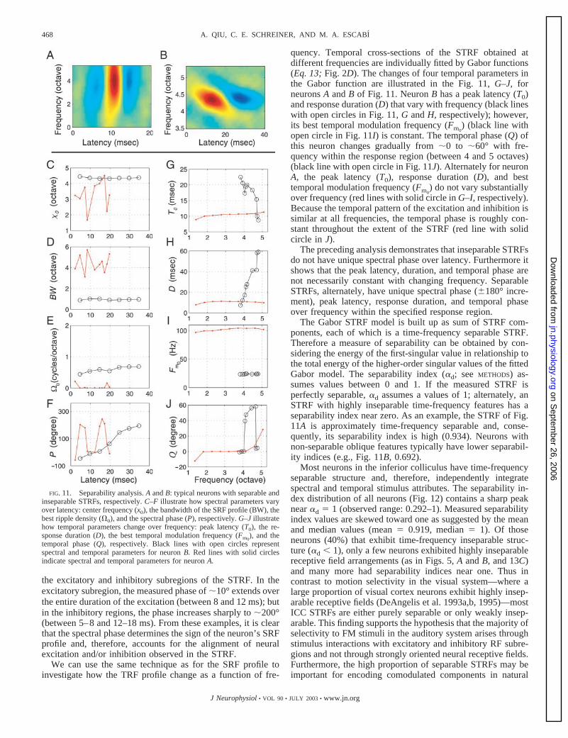
the excitatory and inhibitory subregions of the STRF. In theexcitatory subregion, the measured phase of �10° extends overthe entire duration of the excitation (between 8 and 12 ms); butin the inhibitory regions, the phase increases sharply to �200°(between 5–8 and 12–18 ms). From these examples, it is clearthat the spectral phase determines the sign of the neuron’s SRFprofile and, therefore, accounts for the alignment of neuralexcitation and/or inhibition observed in the STRF.

We can use the same technique as for the SRF profile toinvestigate how the TRF profile change as a function of fre-

quency. Temporal cross-sections of the STRF obtained atdifferent frequencies are individually fitted by Gabor functions(Eq. 13; Fig. 2D). The changes of four temporal parameters inthe Gabor function are illustrated in the Fig. 11, G–J, forneurons A and B of Fig. 11. Neuron B has a peak latency (T0)and response duration (D) that vary with frequency (black lineswith open circles in Fig. 11, G and H, respectively); however,its best temporal modulation frequency (Fm0

) (black line withopen circle in Fig. 11I) is constant. The temporal phase (Q) ofthis neuron changes gradually from �0 to �60° with fre-quency within the response region (between 4 and 5 octaves)(black line with open circle in Fig. 11J). Alternately for neuronA, the peak latency (T0), response duration (D), and besttemporal modulation frequency (Fm0

) do not vary substantiallyover frequency (red lines with solid circle in G–I, respectively).Because the temporal pattern of the excitation and inhibition issimilar at all frequencies, the temporal phase is roughly con-stant throughout the extent of the STRF (red line with solidcircle in J).

The preceding analysis demonstrates that inseparable STRFsdo not have unique spectral phase over latency. Furthermore itshows that the peak latency, duration, and temporal phase arenot necessarily constant with changing frequency. SeparableSTRFs, alternately, have unique spectral phase (180° incre-ment), peak latency, response duration, and temporal phaseover frequency within the specified response region.

The Gabor STRF model is built up as sum of STRF com-ponents, each of which is a time-frequency separable STRF.Therefore a measure of separability can be obtained by con-sidering the energy of the first-singular value in relationship tothe total energy of the higher-order singular values of the fittedGabor model. The separability index (�d; see METHODS) as-sumes values between 0 and 1. If the measured STRF isperfectly separable, �d assumes a values of 1; alternately, anSTRF with highly inseparable time-frequency features has aseparability index near zero. As an example, the STRF of Fig.11A is approximately time-frequency separable and, conse-quently, its separability index is high (0.934). Neurons withnon-separable oblique features typically have lower separabil-ity indices (e.g., Fig. 11B, 0.692).

Most neurons in the inferior colliculus have time-frequencyseparable structure and, therefore, independently integratespectral and temporal stimulus attributes. The separability in-dex distribution of all neurons (Fig. 12) contains a sharp peaknear �d � 1 (observed range: 0.292–1). Measured separabilityindex values are skewed toward one as suggested by the meanand median values (mean � 0.919, median � 1). Of thoseneurons (40%) that exhibit time-frequency inseparable struc-ture (�d � 1), only a few neurons exhibited highly inseparablereceptive field arrangements (as in Figs. 5, A and B, and 13C)and many more had separability indices near one. Thus incontrast to motion selectivity in the visual system—where alarge proportion of visual cortex neurons exhibit highly insep-arable receptive fields (DeAngelis et al. 1993a,b, 1995)—mostICC STRFs are either purely separable or only weakly insep-arable. This finding supports the hypothesis that the majority ofselectivity to FM stimuli in the auditory system arises throughstimulus interactions with excitatory and inhibitory RF subre-gions and not through strongly oriented neural receptive fields.Furthermore, the high proportion of separable STRFs may beimportant for encoding comodulated components in natural

FIG. 11. Separability analysis. A and B: typical neurons with separable andinseparable STRFs, respectively. C–F illustrate how spectral parameters varyover latency: center frequency (x0), the bandwidth of the SRF profile (BW), thebest ripple density (�0), and the spectral phase (P), respectively. G–J illustratehow temporal parameters change over frequency: peak latency (T0), the re-sponse duration (D), the best temporal modulation frequency (Fm0

), and thetemporal phase (Q), respectively. Black lines with open circles representspectral and temporal parameters for neuron B. Red lines with solid circlesindicate spectral and temporal parameters for neuron A.



on Septem


Dow

nloaded from


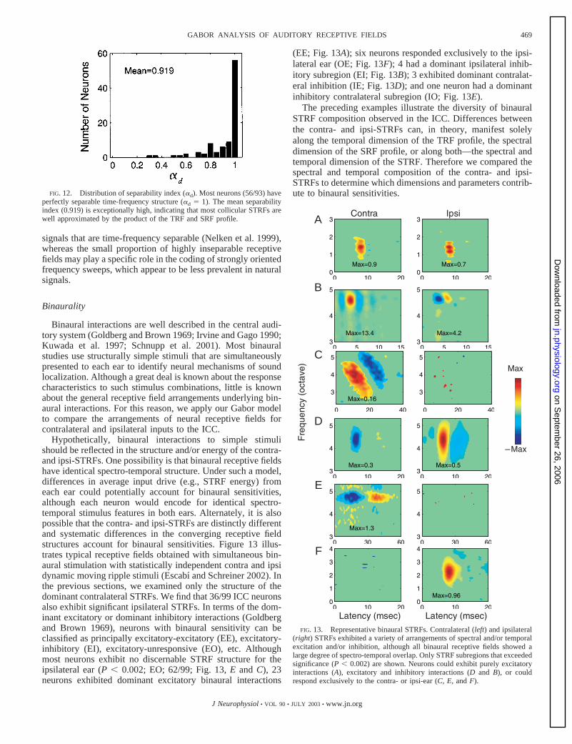
signals that are time-frequency separable (Nelken et al. 1999),whereas the small proportion of highly inseparable receptivefields may play a specific role in the coding of strongly orientedfrequency sweeps, which appear to be less prevalent in naturalsignals.

Binaurality

Binaural interactions are well described in the central audi-tory system (Goldberg and Brown 1969; Irvine and Gago 1990;Kuwada et al. 1997; Schnupp et al. 2001). Most binauralstudies use structurally simple stimuli that are simultaneouslypresented to each ear to identify neural mechanisms of soundlocalization. Although a great deal is known about the responsecharacteristics to such stimulus combinations, little is knownabout the general receptive field arrangements underlying bin-aural interactions. For this reason, we apply our Gabor modelto compare the arrangements of neural receptive fields forcontralateral and ipsilateral inputs to the ICC.

Hypothetically, binaural interactions to simple stimulishould be reflected in the structure and/or energy of the contra-and ipsi-STRFs. One possibility is that binaural receptive fieldshave identical spectro-temporal structure. Under such a model,differences in average input drive (e.g., STRF energy) fromeach ear could potentially account for binaural sensitivities,although each neuron would encode for identical spectro-temporal stimulus features in both ears. Alternately, it is alsopossible that the contra- and ipsi-STRFs are distinctly differentand systematic differences in the converging receptive fieldstructures account for binaural sensitivities. Figure 13 illus-trates typical receptive fields obtained with simultaneous bin-aural stimulation with statistically independent contra and ipsidynamic moving ripple stimuli (Escabı and Schreiner 2002). Inthe previous sections, we examined only the structure of thedominant contralateral STRFs. We find that 36/99 ICC neuronsalso exhibit significant ipsilateral STRFs. In terms of the dom-inant excitatory or dominant inhibitory interactions (Goldbergand Brown 1969), neurons with binaural sensitivity can beclassified as principally excitatory-excitatory (EE), excitatory-inhibitory (EI), excitatory-unresponsive (EO), etc. Althoughmost neurons exhibit no discernable STRF structure for theipsilateral ear (P � 0.002; EO; 62/99; Fig. 13, E and C), 23neurons exhibited dominant excitatory binaural interactions

(EE; Fig. 13A); six neurons responded exclusively to the ipsi-lateral ear (OE; Fig. 13F); 4 had a dominant ipsilateral inhib-itory subregion (EI; Fig. 13B); 3 exhibited dominant contralat-eral inhibition (IE; Fig. 13D); and one neuron had a dominantinhibitory contralateral subregion (IO; Fig. 13E).

The preceding examples illustrate the diversity of binauralSTRF composition observed in the ICC. Differences betweenthe contra- and ipsi-STRFs can, in theory, manifest solelyalong the temporal dimension of the TRF profile, the spectraldimension of the SRF profile, or along both—the spectral andtemporal dimension of the STRF. Therefore we compared thespectral and temporal composition of the contra- and ipsi-STRFs to determine which dimensions and parameters contrib-ute to binaural sensitivities.FIG. 12. Distribution of separability index (�d). Most neurons (56/93) have

perfectly separable time-frequency structure (�d � 1). The mean separabilityindex (0.919) is exceptionally high, indicating that most collicular STRFs arewell approximated by the product of the TRF and SRF profile. A

B

C

D

E

F

–

FIG. 13. Representative binaural STRFs. Contralateral (left) and ipsilateral(right) STRFs exhibited a variety of arrangements of spectral and/or temporalexcitation and/or inhibition, although all binaural receptive fields showed alarge degree of spectro-temporal overlap. Only STRF subregions that exceededsignificance (P � 0.002) are shown. Neurons could exhibit purely excitatoryinteractions (A), excitatory and inhibitory interactions (D and B), or couldrespond exclusively to the contra- or ipsi-ear (C, E, and F).



on Septem


Dow

nloaded from


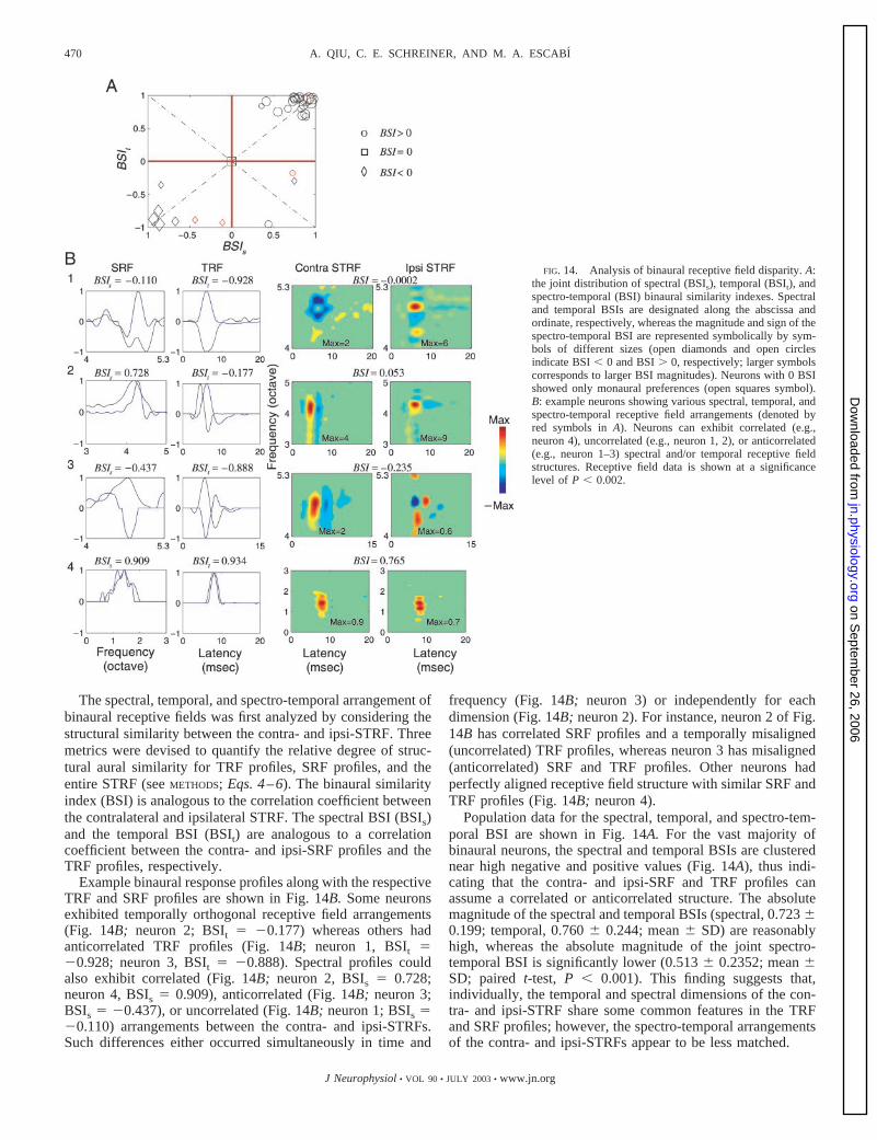
The spectral, temporal, and spectro-temporal arrangement ofbinaural receptive fields was first analyzed by considering thestructural similarity between the contra- and ipsi-STRF. Threemetrics were devised to quantify the relative degree of struc-tural aural similarity for TRF profiles, SRF profiles, and theentire STRF (see METHODS; Eqs. 4–6). The binaural similarityindex (BSI) is analogous to the correlation coefficient betweenthe contralateral and ipsilateral STRF. The spectral BSI (BSIs)and the temporal BSI (BSIt) are analogous to a correlationcoefficient between the contra- and ipsi-SRF profiles and theTRF profiles, respectively.

Example binaural response profiles along with the respectiveTRF and SRF profiles are shown in Fig. 14B. Some neuronsexhibited temporally orthogonal receptive field arrangements(Fig. 14B; neuron 2; BSIt � �0.177) whereas others hadanticorrelated TRF profiles (Fig. 14B; neuron 1, BSIt ��0.928; neuron 3, BSIt � �0.888). Spectral profiles couldalso exhibit correlated (Fig. 14B; neuron 2, BSIs � 0.728;neuron 4, BSIs � 0.909), anticorrelated (Fig. 14B; neuron 3;BSIs � �0.437), or uncorrelated (Fig. 14B; neuron 1; BSIs ��0.110) arrangements between the contra- and ipsi-STRFs.Such differences either occurred simultaneously in time and

frequency (Fig. 14B; neuron 3) or independently for eachdimension (Fig. 14B; neuron 2). For instance, neuron 2 of Fig.14B has correlated SRF profiles and a temporally misaligned(uncorrelated) TRF profiles, whereas neuron 3 has misaligned(anticorrelated) SRF and TRF profiles. Other neurons hadperfectly aligned receptive field structure with similar SRF andTRF profiles (Fig. 14B; neuron 4).

Population data for the spectral, temporal, and spectro-tem-poral BSI are shown in Fig. 14A. For the vast majority ofbinaural neurons, the spectral and temporal BSIs are clusterednear high negative and positive values (Fig. 14A), thus indi-cating that the contra- and ipsi-SRF and TRF profiles canassume a correlated or anticorrelated structure. The absolutemagnitude of the spectral and temporal BSIs (spectral, 0.723 0.199; temporal, 0.760 0.244; mean SD) are reasonablyhigh, whereas the absolute magnitude of the joint spectro-temporal BSI is significantly lower (0.513 0.2352; mean SD; paired t-test, P � 0.001). This finding suggests that,individually, the temporal and spectral dimensions of the con-tra- and ipsi-STRF share some common features in the TRFand SRF profiles; however, the spectro-temporal arrangementsof the contra- and ipsi-STRFs appear to be less matched.

FIG. 14. Analysis of binaural receptive field disparity. A:the joint distribution of spectral (BSIs), temporal (BSIt), andspectro-temporal (BSI) binaural similarity indexes. Spectraland temporal BSIs are designated along the abscissa andordinate, respectively, whereas the magnitude and sign of thespectro-temporal BSI are represented symbolically by sym-bols of different sizes (open diamonds and open circlesindicate BSI � 0 and BSI � 0, respectively; larger symbolscorresponds to larger BSI magnitudes). Neurons with 0 BSIshowed only monaural preferences (open squares symbol).B: example neurons showing various spectral, temporal, andspectro-temporal receptive field arrangements (denoted byred symbols in A). Neurons can exhibit correlated (e.g.,neuron 4), uncorrelated (e.g., neuron 1, 2), or anticorrelated(e.g., neuron 1–3) spectral and/or temporal receptive fieldstructures. Receptive field data is shown at a significancelevel of P � 0.002.



on Septem


Dow

nloaded from


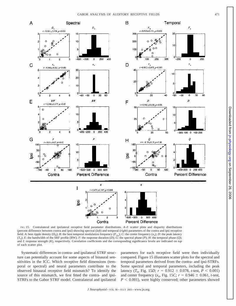
Systematic differences in contra- and ipsilateral STRF struc-ture can potentially account for some aspects of binaural sen-sitivities in the ICC. Which receptive field dimensions (tem-poral or spectral) and neural parameters contribute to theobserved binaural receptive field mismatch? To identify thesource of this mismatch, we first fitted the contra- and ipsi-STRFs to the Gabor STRF model. Contralateral and ipsilateral

parameters for each receptive field were then individuallycompared. Figure 15 illustrates scatter plots for the spectral andtemporal parameters derived from the contra- and ipsi-STRFs.Some spectral and temporal parameters, including the peaklatency (T0, Fig. 15D; r � 0.912 0.078, t-test, P � 0.001)and center frequency (x0, Fig. 15C; r � 0.946 0.061, t-test,P � 0.001), were highly conserved; other parameters showed

FIG. 15. Contralateral and ipsilateral receptive field parameter distributions. A–I: scatter plots and disparity distributions(percent difference between contra and ipsi) showing spectral (left) and temporal (right) parameters of the contra and ipsi receptivefield: A: best ripple density (�0); B: the best temporal modulation frequency (Fm0

); C: the center frequency (x0); D: the peak latency(T0); E: the bandwidth of the SRF profile (BW); F: the response duration (D); G: the spectral phase (P); H: the temporal phase (Q);and I: response strength (K), respectively. Correlation coefficients and the corresponding significance levels are indicated on topof each scatter plot.



on Septem


Dow

nloaded from


lower correlation values although statistically significant.Comparing temporal (Fm0

, D) and spectral parameters (�0,BW), we find that the temporal receptive field dimensions aremore highly matched for the two inputs (Fm0

: r � 0.810 0.111, t-test, P � 0.001; D: r � 0.542 0.158, t-test, P �0.001; �0: r � 0.561 0.156, t-test, P � 0.001; BW: r �0.356 0.177, t-test, P � 0.03). All spectral and temporalparameters were statistically correlated, with the exception ofthe spectral and temporal phases (circular correlation analysis;P: r � 0.01 0.07, bootstrap, P � 0.92; Q: r � �0.10 0.10,bootstrap, P � 0.26). Thus although numerous STRF param-eters collectively contributed to the mismatch of ipsi- andcontra-receptive fields, the spectral and temporal phases con-tributed the most to the binaural receptive field misalignments.Together, this suggests that the overall extent and centers of thespectral and temporal receptive field integration area are typi-cally closely matched binaurally. However, the degree of bin-aural alignment of excitation and inhibition can vary widelyamong neurons, thus providing a currently little appreciatedbinaural integration condition beyond intra-aural time and leveldifferences.

As proposed in the visual system, systematic differences inthe binocular receptive field properties may be used to detectthe depth of a visual object. In the studies by Anzai et al.(1999), visual cortex neurons show systematic differences reti-notopic position and spatial phase between the left and rightinputs that are consistent with models of binocular depth per-ception. Similarly, our analysis of the binaural composition ofthe auditory STRF suggests that differences in the binauralalignment of excitatory and inhibitory RF features may providea mechanism for encoding differences in the converging bin-aural spectrum; which, in turn, can be used to determine theposition of a sound source in space. Unlike visual RFs, we findthat the central position of colliculus STRFs is conservedbinaurally, and therefore positional cues do not appear tocontribute to binaural detection as for the visual system. Sig-nificant disparities in the spectro-temporal phase, however,lead to interleaved patterns of excitation and inhibition binau-rally. Such aural differences may be important for analyzingspectral notches in the spectrum of a sound source, which varysignificantly as a function of spatial position (Hartmann andWitternberg 1996; Kulkarini and Colburn 1998).

D I S C U S S I O N

We have studied the monaural and binaural spectro-temporalreceptive field structure of 99 phase-locking neurons in the catICC (Escabı and Schreiner 2002). A time-frequency GaborSTRF model is presented that allows us to quantify the recep-tive field structure of auditory STRFs. This model can be usedto remove measurement noise in the STRF and to extractphysiologically meaningful information of the receptive fieldstructure. Our results provide the following new insights: 1 theGabor function is an adequate descriptor of the SRF and TRFprofile (Figs. 1 and 2). Using the described singular valuedecomposition method, we can extend the fitting procedure tothe entire STRF. The STRF can be described by the weightedsum of independent separable STRF components, which arethe product of a spectral waveform and a temporal waveform(Figs. 3 and 5). These can in turn be fitted with the time-frequency Gabor STRF model. 2 From the analysis of the

contralateral sMTF and tMTF, ICC neurons exhibited lowpassand/or bandpass spectral and temporal selectivity. 3 The sep-arability index (�d) measures the degree of time-frequencyseparability of the STRF. Most neurons (60.2%) exhibitedtime-frequency separable receptive field structure and, there-fore, independently process spectral and temporal stimulusattributes. 4 Finally, we used the model to study differences inthe converging ipsi- and contralateral receptive field structure.Our results indicate that for neurons exhibiting binaural con-vergence most STRF properties for the two inputs are highlycorrelated. However, subtle spectro-temporal differences in thealignment of excitation and inhibition contribute significantlyto binaural processing in the ICC. Together, the model pro-vides a uniform description of the receptive field structure thatallows us to jointly evaluate spectral, temporal, spectro-tem-poral, and binaural aspects of the stimulus-response relation-ship.

Gabor STRF model

The STRF is an approximation of the neural receptive fieldobtained by the spike-triggered average method using finiteexperimental data (Miller et al. 2002; Escabı and Schreiner2002). A time-frequency Gabor model was used to removemeasurement noise and to quantitatively evaluate the receptivefield structure of ICC neurons. Both the spectral RF andtemporal RF profiles are equally well described by a unidimen-sional Gabor function, as indicated by the high temporal(mean � 0.933) and spectral (mean � 0.938) similarity indicesof the fits to the raw data. The structure of the entire STRFshowed a subtle reduction in the spectro-temporal SI (mean �0.846) that can be accounted for by multiplicative errors thatare propagated independently when the STRF is built up as aproduct of SRF and TRF profiles. Differences in the entireSTRF structure were evaluated by measuring the normalizedMSE between the model and measured STRF. Most neuronshad low MSE values (mean SD � 0.185 0.126; Fig. 6D),indicating that the receptive field structures were well ac-counted for both in shape and energy.

By analyzing the statistical structure of the receptive fieldmeasurement noise (Fig. 4), we were able to determine thenumber of independent receptive field dimensions required toproperly fit collicular STRFs. Typically, we find that one ortwo STRF components are sufficient to capture the structure ofinferior colliculus receptive fields. Only 39.7 and 7.5% of theneurons had significant second and third components eachaccounting, respectively, for only 6.2 5.0 and 2.3 1.8% ofthe total receptive field energy. Because each Gabor functionrequires 9 independent parameters, ICC STRFs therefore typ-ically require 9 or 18 independent parameters to fully accountfor the entire receptive field structure.

Spectro-temporal receptive field structure

The spectral modulation transfer function (sMTF) was usedto quantify the spectral selectivity of the SRF profile. Most ICCneurons exhibited lowpass sMTF (86%, n � 80; 14% band-pass, n � 13) although in most of those cases (70 of 83 lowpassneurons), a non-zero best ripple density (a peak in the filterfunction) could be identified (ranging from 0.022 to 2.113cycles/octave). By comparing the distribution of best ripple



on Septem


Dow

nloaded from


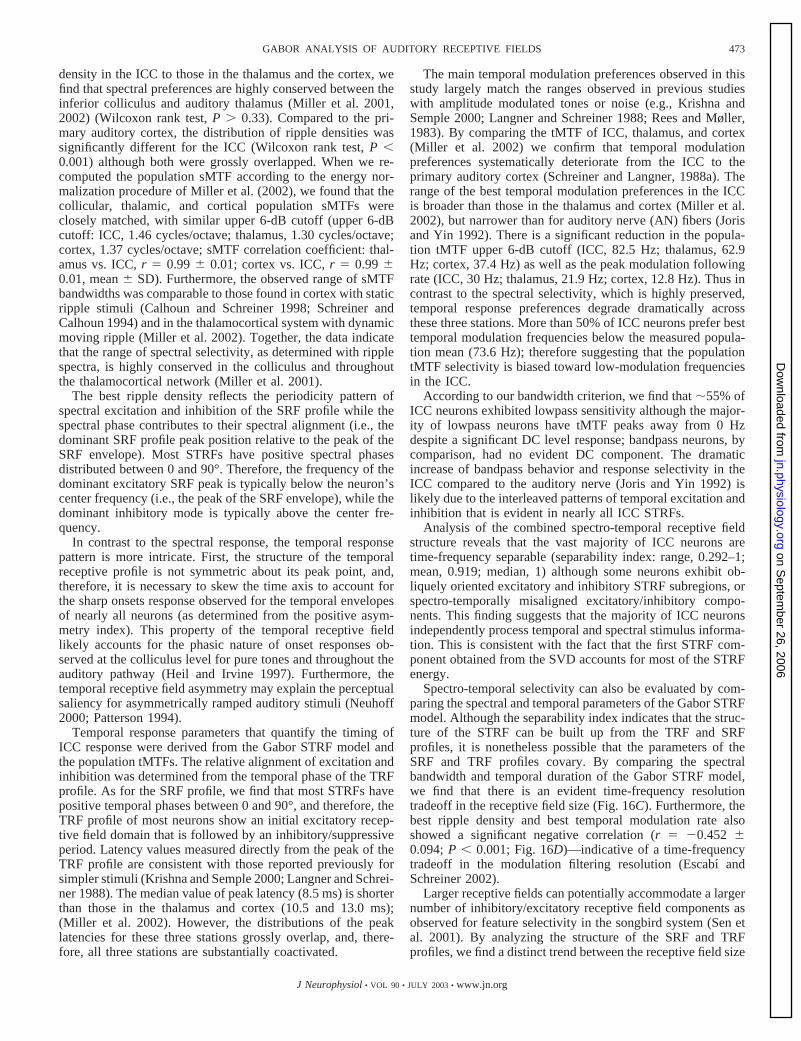
density in the ICC to those in the thalamus and the cortex, wefind that spectral preferences are highly conserved between theinferior colliculus and auditory thalamus (Miller et al. 2001,2002) (Wilcoxon rank test, P � 0.33). Compared to the pri-mary auditory cortex, the distribution of ripple densities wassignificantly different for the ICC (Wilcoxon rank test, P �0.001) although both were grossly overlapped. When we re-computed the population sMTF according to the energy nor-malization procedure of Miller et al. (2002), we found that thecollicular, thalamic, and cortical population sMTFs wereclosely matched, with similar upper 6-dB cutoff (upper 6-dBcutoff: ICC, 1.46 cycles/octave; thalamus, 1.30 cycles/octave;cortex, 1.37 cycles/octave; sMTF correlation coefficient: thal-amus vs. ICC, r � 0.99 0.01; cortex vs. ICC, r � 0.99 0.01, mean SD). Furthermore, the observed range of sMTFbandwidths was comparable to those found in cortex with staticripple stimuli (Calhoun and Schreiner 1998; Schreiner andCalhoun 1994) and in the thalamocortical system with dynamicmoving ripple (Miller et al. 2002). Together, the data indicatethat the range of spectral selectivity, as determined with ripplespectra, is highly conserved in the colliculus and throughoutthe thalamocortical network (Miller et al. 2001).

The best ripple density reflects the periodicity pattern ofspectral excitation and inhibition of the SRF profile while thespectral phase contributes to their spectral alignment (i.e., thedominant SRF profile peak position relative to the peak of theSRF envelope). Most STRFs have positive spectral phasesdistributed between 0 and 90°. Therefore, the frequency of thedominant excitatory SRF peak is typically below the neuron’scenter frequency (i.e., the peak of the SRF envelope), while thedominant inhibitory mode is typically above the center fre-quency.

In contrast to the spectral response, the temporal responsepattern is more intricate. First, the structure of the temporalreceptive profile is not symmetric about its peak point, and,therefore, it is necessary to skew the time axis to account forthe sharp onsets response observed for the temporal envelopesof nearly all neurons (as determined from the positive asym-metry index). This property of the temporal receptive fieldlikely accounts for the phasic nature of onset responses ob-served at the colliculus level for pure tones and throughout theauditory pathway (Heil and Irvine 1997). Furthermore, thetemporal receptive field asymmetry may explain the perceptualsaliency for asymmetrically ramped auditory stimuli (Neuhoff2000; Patterson 1994).

Temporal response parameters that quantify the timing ofICC response were derived from the Gabor STRF model andthe population tMTFs. The relative alignment of excitation andinhibition was determined from the temporal phase of the TRFprofile. As for the SRF profile, we find that most STRFs havepositive temporal phases between 0 and 90°, and therefore, theTRF profile of most neurons show an initial excitatory recep-tive field domain that is followed by an inhibitory/suppressiveperiod. Latency values measured directly from the peak of theTRF profile are consistent with those reported previously forsimpler stimuli (Krishna and Semple 2000; Langner and Schrei-ner 1988). The median value of peak latency (8.5 ms) is shorterthan those in the thalamus and cortex (10.5 and 13.0 ms);(Miller et al. 2002). However, the distributions of the peaklatencies for these three stations grossly overlap, and, there-fore, all three stations are substantially coactivated.

The main temporal modulation preferences observed in thisstudy largely match the ranges observed in previous studieswith amplitude modulated tones or noise (e.g., Krishna andSemple 2000; Langner and Schreiner 1988; Rees and Møller,1983). By comparing the tMTF of ICC, thalamus, and cortex(Miller et al. 2002) we confirm that temporal modulationpreferences systematically deteriorate from the ICC to theprimary auditory cortex (Schreiner and Langner, 1988a). Therange of the best temporal modulation preferences in the ICCis broader than those in the thalamus and cortex (Miller et al.2002), but narrower than for auditory nerve (AN) fibers (Jorisand Yin 1992). There is a significant reduction in the popula-tion tMTF upper 6-dB cutoff (ICC, 82.5 Hz; thalamus, 62.9Hz; cortex, 37.4 Hz) as well as the peak modulation followingrate (ICC, 30 Hz; thalamus, 21.9 Hz; cortex, 12.8 Hz). Thus incontrast to the spectral selectivity, which is highly preserved,temporal response preferences degrade dramatically acrossthese three stations. More than 50% of ICC neurons prefer besttemporal modulation frequencies below the measured popula-tion mean (73.6 Hz); therefore suggesting that the populationtMTF selectivity is biased toward low-modulation frequenciesin the ICC.

According to our bandwidth criterion, we find that �55% ofICC neurons exhibited lowpass sensitivity although the major-ity of lowpass neurons have tMTF peaks away from 0 Hzdespite a significant DC level response; bandpass neurons, bycomparison, had no evident DC component. The dramaticincrease of bandpass behavior and response selectivity in theICC compared to the auditory nerve (Joris and Yin 1992) islikely due to the interleaved patterns of temporal excitation andinhibition that is evident in nearly all ICC STRFs.

Analysis of the combined spectro-temporal receptive fieldstructure reveals that the vast majority of ICC neurons aretime-frequency separable (separability index: range, 0.292–1;mean, 0.919; median, 1) although some neurons exhibit ob-liquely oriented excitatory and inhibitory STRF subregions, orspectro-temporally misaligned excitatory/inhibitory compo-nents. This finding suggests that the majority of ICC neuronsindependently process temporal and spectral stimulus informa-tion. This is consistent with the fact that the first STRF com-ponent obtained from the SVD accounts for most of the STRFenergy.

Spectro-temporal selectivity can also be evaluated by com-paring the spectral and temporal parameters of the Gabor STRFmodel. Although the separability index indicates that the struc-ture of the STRF can be built up from the TRF and SRFprofiles, it is nonetheless possible that the parameters of theSRF and TRF profiles covary. By comparing the spectralbandwidth and temporal duration of the Gabor STRF model,we find that there is an evident time-frequency resolutiontradeoff in the receptive field size (Fig. 16C). Furthermore, thebest ripple density and best temporal modulation rate alsoshowed a significant negative correlation (r � �0.452 0.094; P � 0.001; Fig. 16D)—indicative of a time-frequencytradeoff in the modulation filtering resolution (Escabı andSchreiner 2002).

Larger receptive fields can potentially accommodate a largernumber of inhibitory/excitatory receptive field components asobserved for feature selectivity in the songbird system (Sen etal. 2001). By analyzing the structure of the SRF and TRFprofiles, we find a distinct trend between the receptive field size



on Septem


Dow

nloaded from


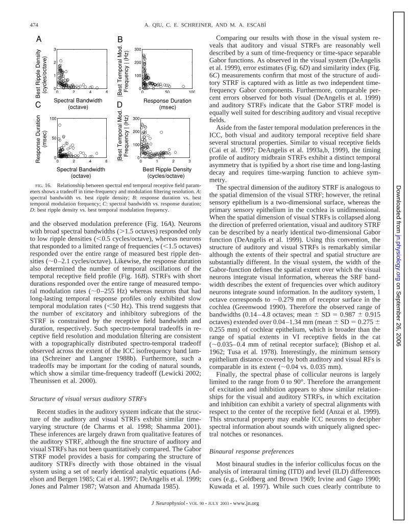
and the observed modulation preference (Fig. 16A). Neuronswith broad spectral bandwidths (�1.5 octaves) responded onlyto low ripple densities (�0.5 cycles/octave), whereas neuronsthat responded to a limited range of frequencies (�1.5 octaves)responded over the entire range of measured best ripple den-sities (�0–2.1 cycles/octave). Likewise, the response durationalso determined the number of temporal oscillations of thetemporal receptive field profile (Fig. 16B). STRFs with shortdurations responded over the entire range of measured tempo-ral modulation rates (�0–255 Hz) whereas neurons that hadlong-lasting temporal response profiles only exhibited slowtemporal modulation rates (�50 Hz). This trend suggests thatthe number of excitatory and inhibitory subregions of theSTRF is constrained by the receptive field bandwidth andduration, respectively. Such spectro-temporal tradeoffs in re-ceptive field resolution and modulation filtering are consistentwith a topographically distributed spectro-temporal tradeoffobserved across the extent of the ICC isofrequency band lam-ina (Schreiner and Langner 1988b). Furthermore, such atradeoffs may be important for the coding of natural sounds,which show a similar time-frequency tradeoff (Lewicki 2002;Theunissen et al. 2000).

Structure of visual versus auditory STRFs

Recent studies in the auditory system indicate that the struc-ture of the auditory and visual STRFs exhibit similar time-varying structure (de Charms et al. 1998; Shamma 2001).These inferences are largely drawn from qualitative features ofthe auditory STRF, although the fine structure of auditory andvisual STRFs has not been quantitatively compared. The GaborSTRF model provides a basis for comparing the structure ofauditory STRFs directly with those obtained in the visualsystem using a set of nearly identical analytic equations (Ad-elson and Bergen 1985; Cai et al. 1997; DeAngelis et al. 1999;Jones and Palmer 1987; Watson and Ahumada 1985).

Comparing our results with those in the visual system re-veals that auditory and visual STRFs are reasonably welldescribed by a sum of time-frequency or time-space separableGabor functions. As observed in the visual system (DeAngeliset al. 1999), error estimates (Fig. 6D) and similarity index (Fig.6C) measurements confirm that most of the structure of audi-tory STRF is captured with as little as two independent time-frequency Gabor components. Furthermore, comparable per-cent errors observed for both visual (DeAngelis et al. 1999)and auditory STRFs indicate that the Gabor STRF model isequally well suited for describing auditory and visual receptivefields.

Aside from the faster temporal modulation preferences in theICC, both visual and auditory temporal receptive field shareseveral structural properties. Similar to visual receptive fields(Cai et al. 1997; DeAngelis et al. 1993a,b, 1999), the timingprofile of auditory midbrain STRFs exhibit a distinct temporalasymmetry that is typified by a short rise time and long-lastingdecay and requires time-warping function to achieve sym-metry.

The spectral dimension of the auditory STRF is analogous tothe spatial dimension of the visual STRF; however, the retinalsensory epithelium is a two-dimensional surface, whereas theprimary sensory epithelium in the cochlea is unidimensional.When the spatial dimension of visual STRFs is collapsed alongthe direction of preferred orientation, visual and auditory STRFcan be described by a nearly identical two-dimensional Gaborfunction (DeAngelis et al. 1999). Using this convention, thestructure of auditory and visual STRFs is remarkably similaralthough the extents of their spectral and spatial structure aresubstantially different. In the visual system, the width of theGabor-function defines the spatial extent over which the visualneurons integrate visual information, whereas the SRF band-width describes the extent of frequencies over which auditoryneurons integrate sound information. In the auditory system, 1octave corresponds to �0.279 mm of receptor surface in thecochlea (Greenwood 1990). Therefore the observed range ofbandwidths (0.14–4.8 octaves; mean SD � 0.987 0.915octaves) extended over 0.04–1.34 mm (mean SD � 0.275 0.255 mm) of cochlear epithelium, which is broader than therange of spatial extents in VI receptive fields in the cat(�0.035–0.4 mm of retinal receptor surface); (Bishop et al.1962; Tusa et al. 1978). Interestingly, the minimum sensoryepithelium distance covered by both auditory and visual RFs iscomparable in its extent (�0.04 vs. 0.035 mm).

Finally, the spectral phase of collicular neurons is largelylimited to the range from 0 to 90°. Therefore the arrangementof excitation and inhibition appears to show similar relation-ships for the visual and auditory STRFs, in which excitationand inhibition can exhibit a variety of spectral alignments withrespect to the center of the receptive field (Anzai et al. 1999).This structural property may enable ICC neurons to decipherspectral information about sounds with uniquely aligned spec-tral notches or resonances.

Binaural response preferences

Most binaural studies in the inferior colliculus focus on theanalysis of interaural timing (ITD) and level (ILD) differencescues (e.g., Goldberg and Brown 1969; Irvine and Gago 1990;Kuwada et al. 1997). While such cues clearly contribute to

FIG. 16. Relationship between spectral end temporal receptive field param-eters shows a tradeoff in time-frequency and modulation filtering resolution. A:spectral bandwidth vs. best ripple density; B: response duration vs. besttemporal modulation frequency; C: spectral bandwidth vs. response duration;D: best ripple density vs. best temporal modulation frequency.



on Septem


Dow

nloaded from


binaural phenomena, little is known about the convergingspectro-temporal receptive field arrangements that contributeto binaural response integration and sound localization in theICC.

By comparing the ipsilateral and contralateral receptivefields derived from simultaneously presented but statisticallyindependent DMR stimuli to the two ears, we were able tocharacterize the structural properties of the converging spectro-temporal information. In � 1⁄3 of the recorded neurons, STRFsfor both ears could be obtained. Individually, the magnitude ofthe spectral and temporal similarity indices can be quite high(mean, 0.738 and 0.816, respectively), whereas the magnitudeof the combined spectro-temporal binaural similarity index istypically much lower (mean � 0.513; paired t-test, P � 0.001).This disparity is partly accounted for by subtle spectral andtemporal phase differences between the SRF or TRF profiles,thus resulting in STRF structures where the contra and ipsiexcitatory and inhibitory subfields are spectro-temporally mis-matched. Although, some of the reduction in the BSI is alsocaused by other STRF parameters that only showed a weakcorrelation (e.g., spectral bandwidth and response duration),the spectral and temporal phases likely provide the greatestcontribution to this reduction (statistically uncorrelated aurally,P � 0.92 and P � 0.26, respectively). Other receptive fieldparameters, including the center frequency, peak latency, bestripple density, and the temporal modulation rate are signifi-cantly correlated. Thus although excitatory and inhibitory in-puts to the ICC are aurally mismatched, their receptive fieldsare centrally overlapped with similar modulation preferences.

Although the magnitude of the spectral and temporal BSIdetermine the correspondence in shape of the contra- andipsi-TRF and -SRF profiles, the sign of the BSI determines therelative alignment of excitation and inhibition. BSI values areclustered for negative and positive values, indicating that SRFand TRF profiles either exhibited a partly correlated or anti-correlated arrangement. The sign of the spectral, temporal, andspectro-temporal BSIs was conserved across all three metrics(Fig. 14A), and therefore, the specific relationship observed forthe STRF (correlated/anticorrelated) was mutually preservedfor the SRF and TRF profiles (spectral vs. spectro-temporal:r � 0.915 0.076, P � 0.001; temporal vs. spectro-temporal:r � 0.853 0.099, P � 0.001). In contrast, the magnitude ofthe spectral and temporal BSIs show no specific correlation(spectral vs. temporal: r � �0.089 0.188; P � 0.5), al-though the magnitude of the spectral and temporal BSIs indi-vidually contributed to the spectro-temporal BSI (spectral vs.spectro-temporal: r � 0.670 0.140, P � 0.001; temporal vs.spectro-temporal: r � 0.531 0.160, P � 0.003).

The binaural receptive field structure should, in theory,account for binaural response preferences of auditory neurons;however, the exact role of the binaural STRF needs to be morefully investigated. Specifically, how does the binaural receptivefield structure contribute to sound localization and binauralphenomena? Because of the slow time course of the TRFprofile (Fig. 9C), it is unlikely that STRF arrangements con-tribute to ITD sensitivities in the ICC (usually in the hun-dredths of microseconds range). Instead, the described recep-tive field arrangements likely contribute to ILD sensitivitiesand location-specific spectral filtering of broadband sound. Thediversity and complexity of observed binaural STRF arrange-ments (e.g., Fig. 13) indicate that simple classification schemes

based on the dominant excitatory or inhibitory receptive fieldcontribution (Goldberg and Brown 1969) are too simplistic tofully account for the binaural preferences to dynamic broad-band stimuli. Differences in the phase, bandwidth, and rippledensity of the SRF structure could potentially be used tolocalize broadband sound sources that are highly susceptible todifferentially filtered spectrum (Hartmann and Witternberg1996; Kulkarini and Colburn 1998). Thus it is possible thatinteraural receptive field disparities are integrated at the col-liculus and beyond to compute the spatial position of a soundsource, analogous to the integration of binocular disparities inthe primary visual cortex (Anzai et al. 1999).

As observed for visual cortex neurons we find that ICCSTRFs share similar structural parameters binaurally althoughtheir spectral and temporal phases appear to be misaligned(Anzai et al. 1999); however, unlike visual receptive fields, wefind no disparities in the central position of the STRF. Therelevance of this finding for sound localization can be under-stood by noting that the binaural detection problem is funda-mentally different from binocular fusion. In the visual system,external visual stimuli can project onto different spatial posi-tions of the retinal epithelium. Deciphering the distance to avisual object requires that visual neurons analyze positionalshifts in the contra and ipsi projecting images and subtle phasedisparities in the local image structure. Sound localization,however, arises via differential filtering of the incoming signalspectrum by the listener’s head and pinnae (Hartmann andWitternberg 1996; Kulkarini and Colburn 1998). This differ-ential filtering modifies the frequency content of the incomingsound by superimposing binaurally misaligned spectral notch-es; yet, unlike the visual system, the sound’s spectral content isnever displaced along the cochlear epithelium. Binaural cuesare, in this manner, interwoven with the frequency spectrum ofthe sound, which is relevant for determining the sound sourcecontent. Thus the observed similarities in the contra and ipsiSTRFs (e.g., center frequency, ripple density, duration etc.)may be important for extracting information about the soundsource content, whereas the misaligned receptive field phasesmay be necessary to decipher interaural disparities arising fromthe sound source position.

Recent studies have demonstrated that binaural STRFs ac-count for much of the structure in spatial selectivity profiles ofcortical neurons (Schnupp et al. 2001), and it is likely that theproposed interaural filtering mechanisms account for the ob-served spatial preferences. The wide assortments of binauralreceptive field arrangements in the colliculus, thalamus, andprimary auditory cortex (Miller et al. 2002) may therefore benecessary for the brain to efficiently compute and decipherdifferences in the incident spectrum, which arise through headshadowing and pinnae filtering and which depend on the soundsource position. Furthermore, temporal differences in the con-tra- and ipsi-STRF structure may be necessary to dynamicallytrack changes in the spectrum of a moving sound source. Suchinteraural filtering, along with the observed receptive fieldarrangements, may provide a basis for encoding binaural dis-parities in the source spectrum independently of contextualinformation in complex environmental stimuli.

We thank Drs. Heather Read and Jose-Manuel Alonso for insightful com-ments.

This work was supported by National Institute of Deafness and Other



on Septem


Dow

nloaded from


Communication Disorders Grant DC-002260 to C. E. Schreiner and a grantfrom the University of Connecticut Research Foundation to M. A. Escabı.

REFERENCES

Adelson EH and Bergen JR. Spatiotemporal energy models for the percep-tion of motion. J Opt Soc Am 2: 284–299, 1985.

Aersten AMHJ, Olders JHJ, and Johannesma PIM. Spectro-temporal re-ceptive fields in auditory neurons in the grass frog: analysis of the stimulus-event relation for tonal stimulus. Biol Cybern 38: 235–248, 1980.

Anzai A, Ohzawa I, and Freeman RD. Neural mechanisms for encodingbinocular disparity: receptive field position versus phase. J Neurophysiol 82:874–890, 1999.

Bishop PO, Kozak W, and Vakkur GJ. Some quantitative aspects of thecat’s eye: axis and plane of reference, visual field co-ordinates and optics.J Physiol 163: 466–502, 1962.

Bliss CI. Statistics in Biology New York: McGraw Hill, 1967.Cai DQ, DeAngelis GC, and Freeman RD. Spatiotemporal receptive field

organization in the lateral geniculate nucleus of cats and kittens. J Neuro-physiol 78: 1045–1061, 1997.

Calhoun B and Schreiner CE. Spectral envelope coding in cat primaryauditory cortex: linear and non-linear effects of stimulus characteristics.J Euro Neurosci 10: 926–940, 1998.

Daugman JG. Uncertainty relation for resolution in space, spatial frequency,and orientation optimized by two-dimensional visual cortical filters. J OptSoc Am A 2: 1160–1169, 1985.

DeAngelis GC, Ghose GM, Ohzawa I, and Freeman RD. Functional micro-organization of primary visual cortex: receptive field analysis of nearbyneurons. J Neurosci 19: 4046–4064, 1999.

DeAngelis GC, Ohzawa I, and Freeman RD. Spatiotemporal organization ofsimple-cell receptive fields in the cat’s striate cortex. I. General character-istics and postnatal development. J Neurophysiol 69: 1091–1117, 1993a.

DeAngelis GC, Ohzawa I, and Freeman RD. Spatiotemporal organization ofsimple-cell receptive fields in the cat’s striate cortex. II. Linearity of tem-poral and spatial summation. J Neurophysiol 69: 1118–1135, 1993b.

DeAngelis GC, Ohzawa I, and Freeman RD. Receptive-field dynamics in thecentral visual pathways. Trends Neurosci 18: 451–458, 1995.

deCharms RC, Blake DT, and Merzenich MM. Optimizing sound featuresfor cortical neurons. Science 280: 1439–1443, 1998.

Depireux DA, Simon JZ, Klein DJ, and Shamma SA. Spectro-temporalresponse field characterization with dynamic ripples in ferret primary audi-tory cortex. J Neurophysiol 85: 1220–1234, 2001.

De Valois RL and Cottaris NP. Inputs to directionally selective simple cellsin macaque striate cortex. Proc Natl Acad Sci USA 95: 14488–14493, 1998.

Efron B and Tibshirani RJ. An Introduction to the Bootstrap. New York:Chapman & Hall, 1993.

Escabı MA and Schreiner CE. Nonlinear spectrotemporal sound analysis byneurons in the auditory midbrain. J Neurosci 22: 4114–4131, 2002.

Goldberg JM and Brown PB. Response of binaural neurons of dog superiorolivary complex to dichotic tonal stimuli: some physiological mechanismsof sound localization. J Neurophysiol 32: 613–636, 1969.

Greenwood D. A cochlear frequency-position function for several spe-cies—29 years later. J Acoust Soc Am 87: 2592–2605, 1990.

Hartmann WM and Wittenberg A. On the externalization of sound images.J Acoust Soc Am 99: 3678–3688, 1996.

Heil P and Irvine DRF. First-spike timing of auditory-nerve fibers andcomparison with auditory cortex. J Neurophysiol 78: 2438–2454, 1997.

Irvine DRF and Gago G. Binaural interaction in high-frequency neurons inthe inferior colliculus of the cat. Effects of variations in sound pressure levelon sensitivity to interaural intensity differences. J Neurophysiol 63: 570–591, 1990.

Jones JP and Palmer LA. An evaluation of the two-dimensional Gabor filtermodel of simple receptive fields in cat striate cortex. J Neurophysiol 58:1233–1258, 1987a.

Jones JP and Palmer LA. The two-dimensional spatial structure of simplereceptive fields in cat striate cortex. J Neurophysiol 58: 1187–1211, 1987b.

Jones JP, Stepnoski A, and Palmer LA. The two-dimensional spectralstructure of simple receptive fields in cat striate cortex. J Neurophysiol 59:1212–1232, 1987.

Joris PX and Yin TCT. Response to amplitude-modulated tones in theauditory nerve. J Acoust Soc Am 91: 215–232, 1992.

Klein DJ, Depireux DA, Simon JZ, and Shamma SA. Robust spectro-temporal reverse correlation for the auditory system: optimizing stimulusdesign. J Comp Neurosci 9: 85–111, 2000.

Kowalski N, Depireux DA, and Shamma SA. Analysis of dynamic spectra inferret primary auditory cortex. I. Characteristics of single-unit responses tomoving ripple spectra. J Neurophysiol 76: 3503–3523, 1996.

Krishna BS and Semple MN. Auditory temporal processing: responses tosinusoidally amplitude-modulated tones in the inferior colliculus. J Neuro-physiol 84: 255–273, 2000.

Kulkarni A and Colburn HS. Role of spectral detail in sound-source local-ization. Nature 396: 747–749, 1998.

Kuwada S, Batra R, Yin TCT, Oliver DL, Haberly LB, and Stanford TR.Intracellular recordings in response to monaural and binaural stimulation of

neurons in the inferior colliculus of the cat. J Neurosci 17: 1565–7581, 1997.Langner G and Schreiner CE. Periodicity coding in the inferior colliculus of

the cat. I. Neuronal mechanisms. J Neurophysiol 60: 1799–1822, 1988.Lewicki MS. Bayesian modeling and classification of neural signals. Neural

Comput 6: 1005–1029, 1994.Lewicki MS. Efficient coding of natural sounds. Nat Neurosci 5: 356–363,

2002.Lu T, Liang L, and Wang X. Neural representation of temporally asymmetric

stimuli in the auditory cortex of awake primates. J Neurophysiol 85: 2364–2380, 2001.

Marcelja S. Mathematical description of the response of simple cortical cells.J Opt Soc Am A 70: 1297–1300, 1980.

Miller LM, Escabı MA, Read HL, and Schreiner CE. Functional conver-gence of response properties in the auditory thalamocortical system. Neuron32: 151–160, 2001.

Miller LM, Escabı MA, Read HL, and Schreiner CE. Spectrotemporalreceptive fields in the lemniscal auditory thalamus and cortex. J Neuro-physiol 87: 516–527, 2002.

Nelken I, Kim PJ, and Young ED. Linear and nonlinear spectral integrationin type IV neurons in the dorsal cochlear nucleus. II. Predicting responseswith the use of nonlinear models. J Neurophysiol 78: 800–811, 1997.

Nelken I, Rotman Y, and Yosef OB. Responses of auditory-cortex neurons tostructural features of natural sounds. Nature 37: 154–157, 1999.

Neuhoff JG. Perceptual bias for rising tones. Nature 395: 123–124, 1998.Patternson RD. The sound of a sinusoid: spectral models. J Acoust Soc Am

96: 1409–1418, 1994.Press WH, Teukolsky SA, Vetterling WT, and Flannery BP. Numerical

Recipes in C (2nd ed.). Cambridge, UK: Cambridge University Press, 1995.Ramachandran R, Davis KA, and May BJ. Single-unit responses in the

inferior colliculus of decerebrate cats. I. Classification based on frequencyresponse maps. J Neurophysiol 82: 152–163, 1999.

Rees A and Møller AR. Responses of neurons in the inferior colliculus of therat to AM and FM tones. Hear Res 10: 301–330, 1983.

Reid RC, Soodak RE, and Shapley RM. Directional selectivity and spatio-temporal structure of receptive fields of simple cells in cat striate cortex.J Neurophysiol 66: 505–529, 1991.

Sen K, Theunissen FE, and Doupe AJ. Feature analysis of natural sounds inthe songbird auditory forebrain. J Neurophysiol 86: 1445–1458, 2001.

Shamma S. On the role of space and time in auditory processing. Trends CognSci 5: 340–348, 2001.

Schnupp JWH, Mrsic-Flogel TD, and King AJ. Linear processing of spatialcues in primary auditory cortex. Nature 414: 200–204, 2001.

Schreiner CE and Calhoun BM. Spectral envelope coding in cat primaryauditory cortex. Aud Neurosci 1: 39–61, 1994.

Schreiner CE and Langner G. Coding of temporal patterns in the centralauditory system. In: Auditory Function: Neurobiological Bases of Hearing.New York: Wiley, 337–362, 1988a.

Schreiner CE and Langner G. Periodicity coding in the inferior colliculus ofthe cat. II. Topographical organization. J Neurophysiol 60: 1823–1840,1988b.

Theunissen FE, Sen K, and Doupe AJ. Spectral-temporal receptive fields ofnonlinear auditory neurons obtained using natural sounds. J Neurosci 20:2315–2331, 2000.

Tusa RJ, Palmer LA, and Rosenquist AC. The retinotopic organization ofArea 17 (striate cortex) in the cat. J Comp Neurol 177: 213–236, 1978.

Versnel H and Shamma SA. Spectral-ripple representation of steady-statevowels in primary auditory cortex. J Acoust Soc Am 103: 2502–2514, 1998.

Watson AB and Ahumada AJ. Model of human visual-motion sensing. J OptSoc Am A 2: 322–342, 1985.



on Septem


Dow

nloaded from


Documents

Gabor Analysis of Auditory Midbrain Receptive Fields ...anqi/journal/escabi_neurophy_2003.pdfGabor Analysis of Auditory Midbrain Receptive Fields: Spectro-Temporal and Binaural Composition