Embed Size (px)
Citation preview
Journal of© Grace Scientific Publishing Statistical Theory and Practice
Volume 2, No.2, June 2008
Gambler’s Ruin with Catastrophes and Windfalls
B. Hunter, Department of Mathematics, University of California,Davis, CA 95616, U.S.A. Email: [email protected]
A.C. Krinik, Department of Mathematics and Statistics,California State Polytechnic University, Pomona, CA 91768,
U.S.A. Email: [email protected]
C. Nguyen, Department of Mathematics and Statistics,California State Polytechnic University, Pomona,
CA 91768, U.S.A. Email: [email protected]
J.M. Switkes, Department of Mathematics and Statistics,California State Polytechnic University, Pomona, CA 91768,
U.S.A. Email: [email protected]
H.F. von Bremen, Department of Mathematics and Statistics,California State Polytechnic University, Pomona, CA 91768,
U.S.A. Email: [email protected]
Received: Sept. 15, 2006 Revised: Feb. 1, 2007
Abstract
We compute ruin probabilities, in both infinite-time and finite-time, for a Gambler’s Ruin prob-lem with both catastrophes and windfalls in addition to the customary win/loss probabilities. Forconstant transition probabilities, the infinite-time ruinprobabilities are derived using difference equa-tions. Finite-time ruin probabilities of a system having constant win/loss probabilities and vari-able catastrophe/windfall probabilities are determined using lattice path combinatorics. Formulaefor expected time till ruin and the expected duration of gambling are also developed. The ruinprobabilities (in infinite-time) for a system having variable win/loss/catastrophe probabilities but nowindfall probability are found. Finally, the infinite-timeruin probabilities of a system with variablewin/loss/catastrophe/windfall probabilities are determined.
AMS Subject Classification: 60J10
Key-words: Gambler’s Ruin, Catastrophe, Birth-Death Process.
1. Introduction
The Gambler’s Ruin problem is over 350 years old and has been traced back to letters be-tween Blaise Pascal and Pierre Fermat; see, for example, Edwards (1983). In the traditional∗1559-8608/08-2/$5 + $1pp – see inside front cover
© Grace Scientific Publishing, LLC
200 B. Hunter, A.C. Krinik, C. Nguyen, J.M. Switkes & H.F. von Bremen
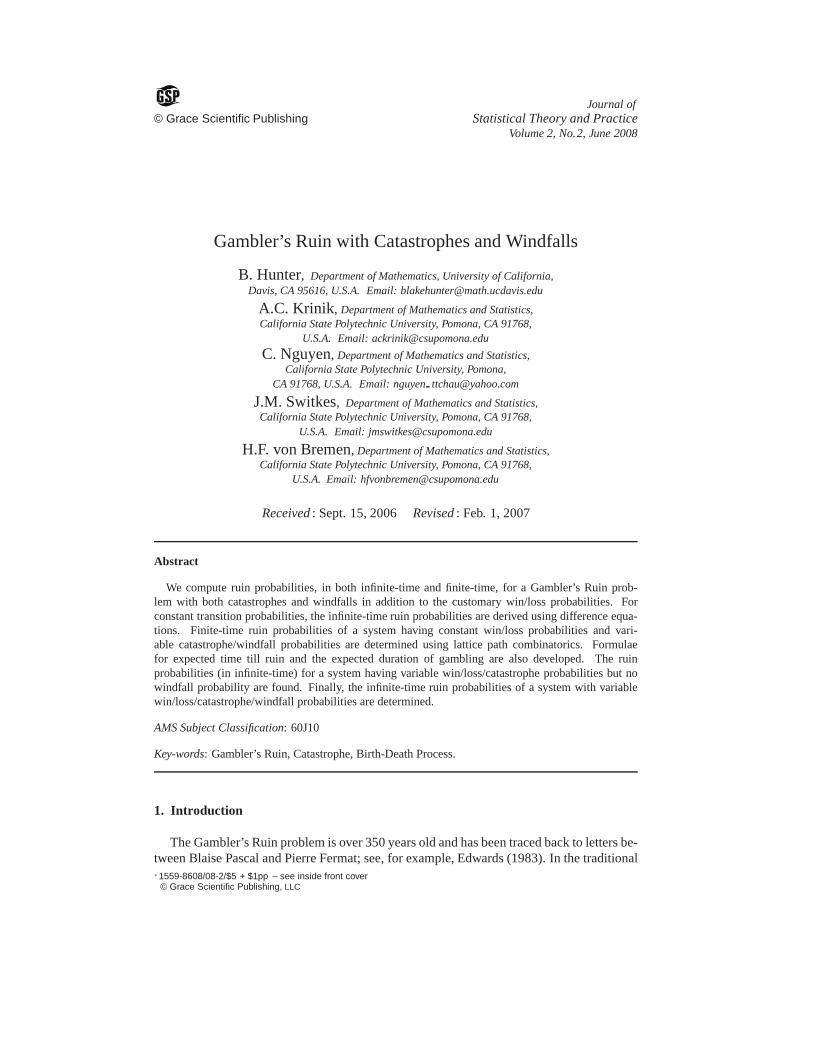
Gambler’s Ruin problem, with two playersP andQ having a total ofH dollars betweenthem, playerP starts with j-dollars, 1≤ j ≤ H −1, and makes a series of independent onedollar bets each having probabilityp of winning a dollar and probabilityq of losing a dollar.PlayerP’s fortune at any point in time may be visualized as a state in the Markov chaindiagram in Figure 1.
j0 1 … … H-1 H
q q q q q
p p p p p 1
1
Figure 1. The state diagram of the traditional Gambler’s Ruin problem
The game ends when playerP loses all of his money or when he reaches his goal ofwinning H dollars. The objective is to determineP’s ruin probability, that is, the chanceof reaching state 0 assuming playerP begins with j-dollars. The most well-known versionof this problem allows play to continue indefinitely until player P reaches state 0 orH.A related problem asks for the ruin probabilities allowing only, at most, a specified, finitenumber of bets. Solutions to both versions of the gambler’s ruin problem date back at least tothe late 1600’s. In addition to Pascal and Fermat, solutionswere obtained by C. Huygens, J.Bernoulli, A. de Moivre, P. de Montmort and N. Bernoulli; see, for example, Edwards (1983)and Takacs (1969). Nicely presented discussions of Gambler’s Ruin problems may also befound in the books by Ash (1970), Feller (1968), and Hoel, Port, and Stone (1987). Aninteresting article by Harper and Ross (2005) reports some recent extensions of gambler’sruin probabilities to different state transition diagrams.
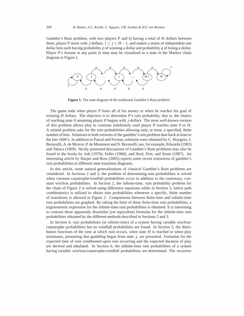
In this article, some natural generalizations of classicalGambler’s Ruin problems areconsidered. In Sections 2 and 3, the problem of determining ruin probabilities is solvedwhen constant catastrophe/windfall probabilities occur in addition to the customary, con-stant win/loss probabilities. In Section 2, the infinite-time, ruin probability problem forthe chain of Figure 2 is solved using difference equations while in Section 3, lattice pathcombinatorics is utilized to obtain ruin probabilities whenever a specific, finite numberof transitions is allowed in Figure 2. Comparisons between finite-time and infinite-timeruin probabilities are graphed. By taking the limit of thesefinite-time ruin probabilities, atrigonometric expression for the infinite-time ruin probabilities is obtained. It is interestingto contrast these apparently dissimilar (yet equivalent) formulae for the infinite-time ruinprobabilities obtained by the different methods describedin Sections 2 and 3.
In Section 4, ruin probabilities (in infinite-time) of a system having variable win/loss/catastrophe probabilities but no windfall probabilities are found. In Section 5, the distri-bution functions of the time at which ruin occurs, when stateH is reached or when playterminates, presuming that gambling began from statej, are presented. Formulae for theexpected time of ruin conditioned upon ruin occurring and the expected duration of playare derived and tabulated. In Section 6, the infinite-time ruin probabilities of a systemhaving variable win/loss/catastrophe/windfall probabilities are determined. The recursive
Gambler’s Ruin with Catastrophes and Windfalls 201
q+c
0 1 j… … HH-1
q q q q
p p p p p+w
11
c
w w w w
ccc
Figure 2. Transition state diagram of Gambler’s Ruin with constant catastropheand windfall probabilities
approaches in Sections 4 and 6 generalize the known ruin probability formula in Hoel, Port,and Stone (1987) for general birth-death chains. If the systems described in Sections 2, 4and 6 are changed to include return transition probabilities (loops), then the same recursivemethods, suitably modified, still produce formulae for computing ruin probabilities. Thisresult and some related problems and directions for furtherstudy are mentioned in Section 7.
2. Infinite-time Gambler’s ruin probabilities with catastr ophes and windfalls
Suppose that in each round of a Gambler’s Ruin game playerP wins with probabilityp, loses with probabilityq, experiences a catastrophe taking him or her to state 0 withprobabilityc, and gains a windfall taking him or her to stateH with probabilityw, wherep+q+c+w= 1, as shown in the Markov chain state diagram in Figure 2.
Let infinite-time ruin probabilities be given by
rk = Prob(P is eventually ruined| P is initially at statek).
Suppose that playerP currently hask dollars, where 1≤ k ≤ H − 1. Conditioning on thenext round of play, with probabilityc playerP will go directly to state 0 and be ruined; withprobabilityq playerP will go to statek−1, from which he or she has probabilityrk−1 ofeventual ruin; with probabilityp playerP will go to statek+ 1, from which he or she hasprobabilityrk+1 of eventual ruin; and with probabilityw playerP will go directly to stateH,from which he or she has no chance of being ruined.
202 B. Hunter, A.C. Krinik, C. Nguyen, J.M. Switkes & H.F. von Bremen
Thus, for 1≤ k≤ H −1,
rk = cr0 +qrk−1 + prk+1+wrH
= c+qrk−1+ prk+1,
where we have used the fact thatr0 = 1 (since the player is already ruined in this case) andrH = 0 (since upon reaching stateH the player stops playing the game). That is,
r0 = 1
r1 = c+qr0+ pr2
r2 = c+qr1+ pr3
...
rk = c+qrk−1+ prk+1 (2.1)...
rH−1 = c+qrH−2+ prH
rH = 0.
This is a set of linear constant-coefficient difference equations with “boundary values”r0 = 1 andrH = 0. In other words, we are looking for the solution of
prk+1− rk +qrk−1 = −c (2.2)
subject to the “boundary values”r0 = 1 andrH = 0. The general solution of (2.2) may befound as a sum of the general solution of the associated homogeneous equation
prk+1− rk +qrk−1 = 0 (2.3)
and a particular solution of the non-homogeneous equation (2.2), see Goldberg (1986) andMarcus (1998).
To find a particular solution of (2.2), we will assumerk = A whereA is a constant. Thensubstituting into (2.2),
pA−A+qA= −c
and we obtainrk = cc+w, for all k.
For the homogeneous equation (2.3), the characteristic polynomial is px2− x+ q. Theroots of the characteristic polynomial are(1±√
1−4pq)/(2p). Thus, forpq 6= 1/4, thegeneral solution of the non-homogeneous equation (2.2) is
rk = C1
[
1+√
1−4pq2p
]k
+C2
[
1−√1−4pq2p
]k
+c
c+w. (2.4)
Applying the initial conditions,r0 = 1 andrH = 0, we have that the ruin probabilities (forpq 6= 1
4) are given by
rk =c
c+w+
[
− c(2p)H +w(1−√1−4pq)H
(c+w)[(1+√
1−4pq)H − (1−√1−4pq)H ]
]
·[
1+√
1−4pq2p
]k
Gambler’s Ruin with Catastrophes and Windfalls 203
+
[
1− cc+w
+c(2p)H +w(1−√
1−4pq)H
(c+w)[(1+√
1−4pq)H − (1−√1−4pq)H ]
]
·[
1−√1−4pq2p
]k
. (2.5)
In the special case of catastrophes but no windfalls (w = 0), again assumingpq 6= 14, this
result reduces to
rk = 1−
[
1+√
1−4pq2p
]k
−[
1−√1−4pq2p
]k
[
1+√
1−4pq2p
]H
−[
1−√1−4pq2p
]H , for w = 0. (2.6)
We can use the Binomial Theorem to re-write thisw = 0 result without using radicals:
(
1+√
x)k
=k
∑i=0
(
ki
)
(√x)i
(
1−√
x)k
=k
∑i=0
(−1)i(
ki
)
(√x)i
(
1+√
x)k−
(
1−√
x)k
= 2k
∑i=1i odd
(
ki
)
(√x)i
= 2√
x⌊ k−1
2 ⌋
∑j=0
(
k2 j +1
)
x j
where⌊y⌋ denotes the greatest integer≤ y. The resulting alternative form for the ruin prob-abilities withw = 0 (and still assumingpq 6= 1/4) is
rk = 1−
(2p)H−k ·
⌊ k−12 ⌋
∑j=0
(
k2 j +1
)
(1−4pq) j
⌊H−12 ⌋
∑j=0
(
H2 j +1
)
(1−4pq) j
, for w = 0, pq 6= 1/4. (2.7)
In the special case of no catastrophes or windfalls (c = w = 0), for the moment stillassumingpq 6= 1
4, the result in (2.6) reduces even further. The roots of the characteristicpolynomial becomeqp and 1, and we obtain ruin probabilities
rk =
(
qp
)H−(
qp
)k
(
qp
)H−1
, for c = w = 0, pq 6= 14. (2.8)
Finally, in the special case in whichp= q= 12, the characteristic polynomial has a double
root of 1. In this case, the general solution has the form
rk = C1 +C2k. (2.9)
204 B. Hunter, A.C. Krinik, C. Nguyen, J.M. Switkes & H.F. von Bremen
0
0.1
0.2
0.3
0.4
0.5
0.6
0.7
0.8
0.9
1
1 2 3 4 5 6 7 8 9 10 11 12 13 14 15 16
p=0.4, q=0.6
p=0.5, q=0.5
p=0.45, q=0.45,
w=0.1
p=0.4, q=0.4,
c=0.1, w=0.1
rk
k
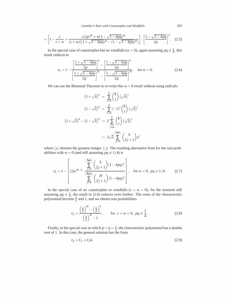
Figure 3. Infinite-time ruin probabilities withH = 16 for several sets ofp,q, c, w values withp+q+c+w = 1
Applying the initial conditions, we obtain ruin probabilities
rk = 1− kH
, for p = q =12. (2.10)
We have thus fully characterized the ruin probabilities in infinite time with constant-ratecatastrophes and windfalls.
In Figure 3, we illustrate infinite-time ruin probabilitieswith H = 16 for several sets ofp, q, c, w values withp+ q+ c+ w = 1. Note the effects of loss of symmetry as shownin the uppermost and lowest curves, as well as the effects of introducing catastrophes andwindfalls in a symmetric manner as shown in the middle non-linear curve. We turn next toruin probabilities in finite time.
3. Finite-time ruin probabilities with catastrophes and windfalls
Let finite-step ruin probabilities be given by
r(n)k = Prob(P is ruined in firstn steps| P is initially at statek).
In this section, we continue to assume thatp+q+c+w= 1.
Let
L(n)k, j = number of paths from statek to statej in n steps,
where 1≤ j ≤H−1 and 1≤ k≤H−1 and the paths are restricted from hitting the absorbingstates at 0 andH. It is shown in Mohanty (1979) and Narayana (1979) that
L(n)k, j =
H+1
∑i=1
[(
nn− j+k
2 − i(H +1)
)
−(
nn+ j+k−2
2 + i(H +1)+1
)]
(3.1a)
Gambler’s Ruin with Catastrophes and Windfalls 205
and in Kriniket al. (2005) and Takacs (1969) that
L(n)k, j =
2H
H
∑u=1
sin
(
uπ jH
)
sin
(
uπkH
)
[
2cos(uπ
H
)]n. (3.1b)
We use the convention that binomial coefficients(a
b
)
are defined to be 0 ifb > a or b < 0 orif neithera norb is integer-valued.
While it is not even obvious that (3.1b) is integer-valued, it does in fact count the numberof paths.
Let
P(n)k, j = Prob(P is at statej at nth step| P is initially at statek).
Assuming 1≤ j ≤ H −1 and 1≤ k≤ H −1,
P(n)k, j = L(n)
k, j p(n+ j−k)/2q(n− j+k)/2, (3.2)
where the exponents onp andq ensure thatn steps are taken in such a way that the netchange in position isj − k. That is,(n+ j − k)/2+(n− j + k)/2 = n and(n+ j − k)/2−(n− j +k)/2= j −k. Substituting (3.1b) into (3.2),
P(n)k, j =
2H
p( j−k)/2q(k− j)/2H
∑u=1
sin
(
uπ jH
)
sin
(
uπkH
)
[
2√
pqcos(uπ
H
)]n(3.3)
for 1≤ j ≤ H −1 and 1≤ k≤ H −1.
Now, for n > 0,
r(n)k =
n−1
∑i=0
P(i)k,1 ·q+
n−1
∑i=0
H−1
∑j=1
P(i)k, j ·c. (3.4)
This follows from the fact that in order to reach state 0, either a) after some number ofsteps we reached state 1 and then took an immediate step down to state 0, or b) after somenumber of steps we reached statej and then experienced a catastrophe taking us to state 0;see Hunter (2005) for more details. Using (3.3) in (3.4) we obtain, for 1≤ k ≤ H −1, thefinite-time ruin probabilities
r(n)k =
n−1
∑i=0
2H
p(i−k+1)/2q(i+k−1)/2H
∑u=1
sin(uπ
H
)
sin
(
uπkH
)
[
2cos(uπ
H
)]i·q
+n−1
∑i=0
H−1
∑j=1
2H
p(i+ j−k)/2q(i+k− j)/2H
∑u=1
sin
(
uπ jH
)
sin
(
uπkH
)
[
2cos(uπ
H
)]i·c (3.5)
For completeness we may also give the trivial resultsr(n)0 = 1 andr(n)
H = 0.
In the limit asn→ ∞, the result in (3.5) should reduce to the result in (2.5). While thisappears difficult to prove analytically, in what follows we derive one form for (3.5) in thelimit as n → ∞. We assumepq 6= 1
4 (that is, pq< 14 sincep+ q+ c+ w= 1) as this was
assumed in (2.5).
206 B. Hunter, A.C. Krinik, C. Nguyen, J.M. Switkes & H.F. von Bremen
As a first step, we change the order of summations and rearrange factors in (3.5):
r(n)k =
2√
pq
H
(√
qp
)k
·H
∑u=1
sin(uπ
H
)
sin
(
uπkH
)n−1
∑i=0
[
2√
pqcos(uπ
H
)]i
+2cH
(√
qp
)k
·H−1
∑j=1
(√
pq
)j H
∑u=1
sin
(
uπ jH
)
sin
(
uπkH
)n−1
∑i=0
[
2√
pqcos(uπ
H
)]i(3.6)
Now, in the limit asn → ∞, the summation with respect toi is a convergent geometricseries since 2
√pqcos
(
uπH
)
< 1 for pq 6= 14. Thus, we obtain a new form for the infinite-time
ruin probabilities for 1≤ k≤ H −1 with pq 6= 14:
rk = limn→∞
r(n)k
=2√
pq
H
(√
qp
)k
·H
∑u=1
sin(
uπH
)
sin(
uπkH
)
1−2√
pqcos(
uπH
) (3.7)
+2cH
(√
qp
)k
·H−1
∑j=1
(√
pq
) j H
∑u=1
sin(
uπ jH
)
sin(
uπkH
)
1−2√
pqcos(
uπH
)
We have confirmed numerically that (3.7) is equivalent to (2.5).
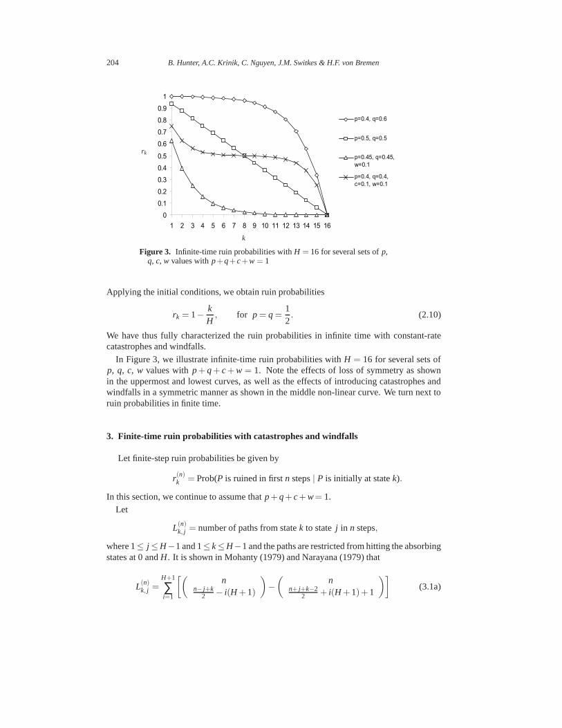
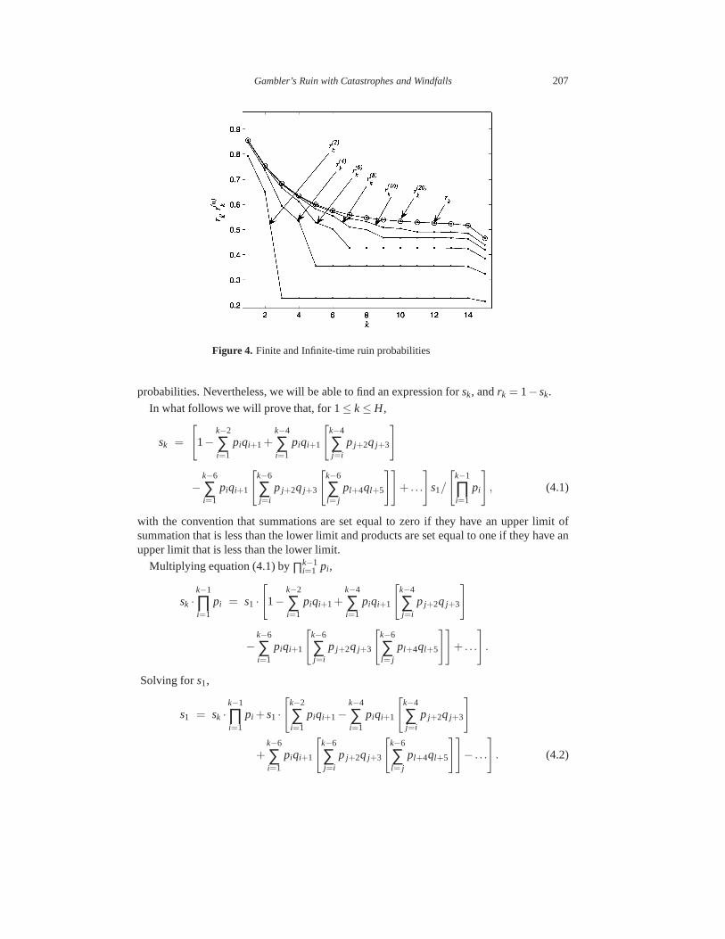
In the example illustrated in Figure 4, we see that the finite-time ruin probabilities withcatastrophes and windfalls (equation (3.5)) converge to the infinite-time ruin probabilities(equation (2.5)) as the number of steps,n, is increased. In the example we letp = 0.1,q = 0.65,c = 0.13,w = 0.12 andH = 16. Figure 4 shows the computed finite and infinite-time ruin probabilities for the above-mentioned parameters. The finite ruin probabilitiesare shown for number of steps of 2,4,6,8,10 and 20. As the number of steps increases,the finite-time ruin probabilities converge to the infinite-time ruin probabilities. Within the
resolution of the graph,r(20)k andrk are indistinguishable.
4. Infinite-time Gambler’s ruin probabilities with variabl e win/loss/catastropheprobabilities and no windfalls
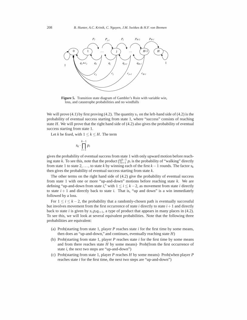
Suppose now that the transition probabilities are state-dependent withpk, qk, ck, andwk
representing probabilities associated with statek. Suppose also that there are no windfalls(wk = 0 for all k) so that for 1≤ k ≤ H −1, pk + qk + ck = 1. The corresponding Markovchain diagram is shown in Figure 5.
As before, let infinite-time ruin probabilities be given by
rk = Prob(P is eventually ruined| P is initially at statek).
Also define “success” probabilities by
sk = Prob(P is eventually absorbed at stateH | P is initially at statek) = 1− rk.
The difference equations corresponding tork or sk no longer involve constant transition
Gambler’s Ruin with Catastrophes and Windfalls 207
Figure 4. Finite and Infinite-time ruin probabilities
probabilities. Nevertheless, we will be able to find an expression forsk, andrk = 1−sk.
In what follows we will prove that, for 1≤ k≤ H,
sk =
[
1−k−2
∑i=1
piqi+1 +k−4
∑i=1
piqi+1
[
k−4
∑j=i
p j+2q j+3
]
−k−6
∑i=1
piqi+1
[
k−6
∑j=i
p j+2q j+3
[
k−6
∑l= j
pl+4ql+5
]]
+ . . .
]
s1/
[
k−1
∏i=1
pi
]
, (4.1)
with the convention that summations are set equal to zero if they have an upper limit ofsummation that is less than the lower limit and products are set equal to one if they have anupper limit that is less than the lower limit.
Multiplying equation (4.1) by∏k−1i=1 pi ,
sk ·k−1
∏i=1
pi = s1 ·[
1−k−2
∑i=1
piqi+1+k−4
∑i=1
piqi+1
[
k−4
∑j=i
p j+2q j+3
]
−k−6
∑i=1
piqi+1
[
k−6
∑j=i
p j+2q j+3
[
k−6
∑l= j
pl+4ql+5
]]
+ . . .
]
.
Solving fors1,
s1 = sk ·k−1
∏i=1
pi +s1 ·[
k−2
∑i=1
piqi+1−k−4
∑i=1
piqi+1
[
k−4
∑j=i
p j+2q j+3
]
+k−6
∑i=1
piqi+1
[
k−6
∑j=i
p j+2q j+3
[
k−6
∑l= j
pl+4ql+5
]]
− . . .
]
. (4.2)
208 B. Hunter, A.C. Krinik, C. Nguyen, J.M. Switkes & H.F. von Bremen
q1+c1
0 1 j… … HH-1
q2 qj qj+1 qH-1
p1
11
cH-1cj+1cjc2
Pj-1pj pH-2 pH-1
Figure 5. Transition state diagram of Gambler’s Ruin with variable win,loss, and catastrophe probabilities and no windfalls
We will prove (4.1) by first proving (4.2). The quantitys1 on the left-hand side of (4.2) is theprobability of eventual success starting from state 1, where “success” consists of reachingstateH. We will prove that the right hand side of (4.2) also gives theprobability of eventualsuccess starting from state 1.
Let k be fixed, with 1≤ k≤ H. The term
sk ·k−1
∏i=1
pi
gives the probability of eventual success from state 1 with only upward motion before reach-ing statek. To see this, note that the product∏k−1
i=1 pi is the probability of “walking” directlyfrom state 1 to state 2, . . . , to statek by winning each of the firstk−1 rounds. The factorsk
then gives the probability of eventual success starting from statek.
The other terms on the right hand side of (4.2) give the probability of eventual successfrom state 1 with one or more “up-and-down” motions before reaching statek. We aredefining “up-and-down from statei,” with 1 ≤ i ≤ k−2, as movement from statei directlyto statei + 1 and directly back to statei. That is, “up and down” is a win immediatelyfollowed by a loss.
For 1≤ i ≤ k− 2, the probability that a randomly-chosen path is eventually successfulbut involves movement from the first occurrence of statei directly to statei +1 and directlyback to statei is given bys1piqi+1, a type of product that appears in many places in (4.2).To see this, we will look at several equivalent probabilities. Note that the following threeprobabilities are equivalent:
(a) Prob(starting from state 1, playerP reaches statei for the first time by some means,then does an “up-and-down,” and continues, eventually reaching stateH)
(b) Prob(starting from state 1, playerP reaches statei for the first time by some meansand from there reaches stateH by some means)· Prob(from the first occurrence ofstatei, the next two steps are “up-and-down”)
(c) Prob(starting from state 1, playerP reachesH by some means)· Prob(when playerPreaches statei for the first time, the next two steps are “up-and-down”)
Gambler’s Ruin with Catastrophes and Windfalls 209
Note that (a), (b), and (c) are all equal tos1piqi+1 sinces1 is the probability of eventualsuccessful movement to stateH from initial state 1 andpiqi+1 is the probability that fromthe first occurrence of statei the next two steps are “up-and-down.”
Now the sum multiplyings1 on the right-hand side of (4.2),
k−2
∑i=1
piqi+1−k−4
∑i=1
piqi+1
[
k−4
∑j=i
p j+2q j+3
]
+k−6
∑i=1
piqi+1
[
k−6
∑j=i
p j+2q j+3
[
k−6
∑l= j
pl+4ql+5
]]
− . . . ,
is simply an application of the Inclusion/Exclusion Principle giving the probability of even-tual success from state 1 with some “up-and-down” motion before reaching statek, wherekis fixed with 1≤ k≤ H. The first summation in this sum,
k−2
∑i=1
piqi+1,
gives the sum of the probabilities that from statei, the next two steps are “up-and-down,” forstatesi from 1 tok−2. (If we let i reachk−1, the “up-and-down” would take us to statekon its “up,” resulting in this “up-and-down” not being completed before the first occurrenceof statek.) However, for non-adjacent statesi, j, it is possible for a path to success to havean “up-and-down” motion at the first occurrence of both statei and statej. The doublesummation
k−4
∑i=1
piqi+1
[
k−4
∑j=i
p j+2q j+3
]
is subtracted, since it is the sum of probabilities of “up-and-down” motions at the first oc-currences of two different (non-adjacent) states. The upper limit of summation has beendecreased tok−4 to allow “space” for both “up-and-downs” to occur at states≤ k−2. Thetriple summation
k−6
∑i=1
piqi+1
[
k−6
∑j=i
p j+2q j+3
[
k−6
∑l= j
pl+4ql+5
]]
then is added back, since it is the sum of probabilities of “up-and-downs” occurring at thefirst occurrences of three different (pairwise non-adjacent) states. This Inclusion/Exclusionis continued in order to compute correctly a quantity that, when multiplied bys1, givesthe probability of eventual success from state 1 with some “up-and-down” motions beforereaching statek for the first time. Adding the first term on the right hand side of (4.2), weobtain the total probability of success from initial state 1, with or without “up-and-down”motions before reaching statek for the first time, as given on the left-hand side of (4.2). Thiscompletes the proof of (4.2), and thus also of (4.1).
210 B. Hunter, A.C. Krinik, C. Nguyen, J.M. Switkes & H.F. von Bremen
Now, settingk = H in (4.1) and recalling thatsH = 1,
sH =
[
1−H−2
∑i=1
piqi+1 +H−4
∑i=1
piqi+1
[
H−4
∑j=i
p j+2q j+3
]
−H−6
∑i=1
piqi+1
[
H−6
∑j=i
p j+2q j+3
[
H−6
∑l= j
pl+4ql+5
]]
+ . . .
]
s1/
[
H−1
∏i=1
pi
]
= 1.
This allows us to solve fors1, obtaining
s1 =
[
H−1
∏i=1
pi
]
/
[
1−H−2
∑i=1
piqi+1 +H−4
∑i=1
piqi+1
[
H−4
∑j=i
p j+2q j+3
]
−H−6
∑i=1
piqi+1
[
H−6
∑j=i
p j+2q j+3
[
H−6
∑l= j
pl+4ql+5
]]
+ . . .
]
.
Finally, this in turn implies by (4.1) that
sk =
1−k−2∑
i=1piqi+1 +
k−4∑
i=1piqi+1
[
k−4∑j=i
p j+2q j+3
]
− . . .
1−H−2∑
i=1piqi+1 +
H−4∑
i=1piqi+1
[
H−4∑j=i
p j+2q j+3
]
− . . .
·H−1
∏i=k
pi .
The ruin probabilities, for 1≤ k≤ H, are therefore given by
rk = 1−
1−k−2∑
i=1piqi+1 +
k−4∑
i=1piqi+1
[
k−4∑j=i
p j+2q j+3
]
− . . .
1−H−2∑
i=1piqi+1 +
H−4∑
i=1piqi+1
[
H−4∑j=i
p j+2q j+3
]
− . . .
·H−1
∏i=k
pi .
We turn next to questions of duration of play.
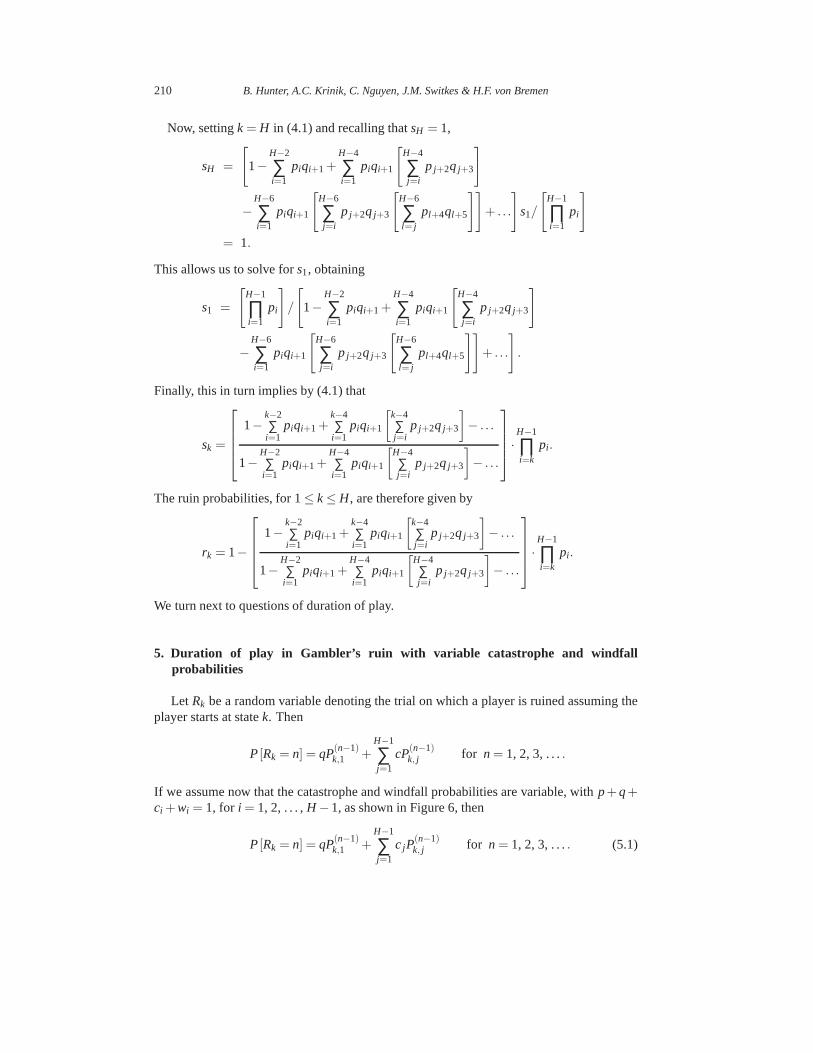
5. Duration of play in Gambler’s ruin with variable catastro phe and windfallprobabilities
Let Rk be a random variable denoting the trial on which a player is ruined assuming theplayer starts at statek. Then
P[Rk = n] = qP(n−1)k,1 +
H−1
∑j=1
cP(n−1)k, j for n = 1, 2, 3, . . ..
If we assume now that the catastrophe and windfall probabilities are variable, withp+q+ci +wi = 1, for i = 1, 2, . . . ,H −1, as shown in Figure 6, then
P[Rk = n] = qP(n−1)k,1 +
H−1
∑j=1
c jP(n−1)k, j for n = 1, 2, 3, . . .. (5.1)
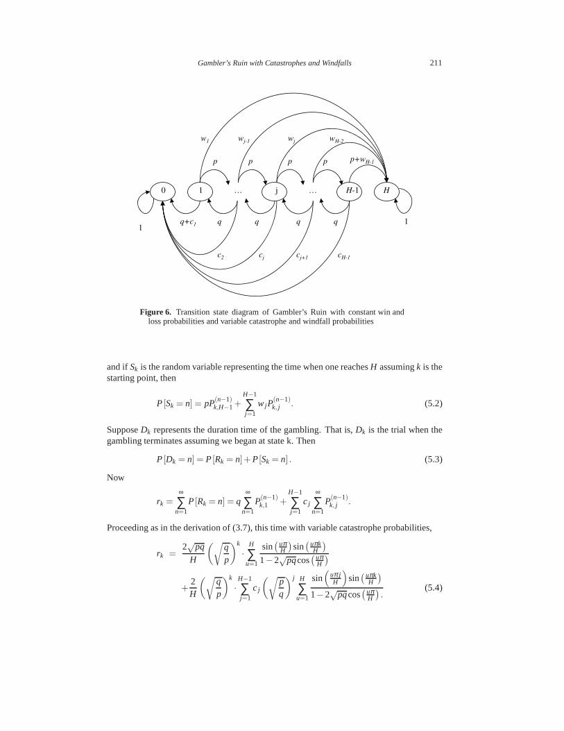
Gambler’s Ruin with Catastrophes and Windfalls 211
q+c1
0 1 j… … HH-1
q q q q
p p p p
11
w1 wj-1 wj wH-2
p+wH-1
c2 cj cj+1 cH-1
Figure 6. Transition state diagram of Gambler’s Ruin with constant win andloss probabilities and variable catastrophe and windfall probabilities
and ifSk is the random variable representing the time when one reachesH assumingk is thestarting point, then
P[Sk = n] = pP(n−1)k,H−1 +
H−1
∑j=1
wj P(n−1)k, j . (5.2)
SupposeDk represents the duration time of the gambling. That is,Dk is the trial when thegambling terminates assuming we began at state k. Then
P[Dk = n] = P[Rk = n]+P[Sk = n] . (5.3)
Now
rk =∞
∑n=1
P[Rk = n] = q∞
∑n=1
P(n−1)k,1 +
H−1
∑j=1
c j
∞
∑n=1
P(n−1)k, j .
Proceeding as in the derivation of (3.7), this time with variable catastrophe probabilities,
rk =2√
pq
H
(√
qp
)k
·H
∑u=1
sin(
uπH
)
sin(
uπkH
)
1−2√
pqcos(
uπH
)
+2H
(√
qp
)k
·H−1
∑j=1
c j
(√
pq
) j H
∑u=1
sin(
uπ jH
)
sin(
uπkH
)
1−2√
pqcos(
uπH
)
.(5.4)
212 B. Hunter, A.C. Krinik, C. Nguyen, J.M. Switkes & H.F. von Bremen
Note that (5.4) still applies ifp = q = 1/2.
Similarly,
sk =∞
∑n=1
P[Sk = n]
= p∞
∑n=1
P(n−1)k,H−1 +
H−1
∑j=1
wj
∞
∑n=1
P(n−1)k, j .
After a derivation similar to that used in obtaining (3.7), we find
sk =2√
pq
H
(√
qp
)k
·(√
pq
)H
·H
∑u=1
sin(
uπ(H−1)H
)
sin(
uπkH
)
1−2√
pqcos(
uπH
)
+2H
(√
qp
)k
·H−1
∑j=1
wj
(√
pq
) j H
∑u=1
sin(
uπ jH
)
sin(
uπkH
)
1−2√
pqcos(
uπH
) . (5.5)
Note that if p+ q+ ci + wi = 1 for i = 1, 2, . . . ,H −1, then 1− rk = sk. However, equa-tions (5.1), (5.2), (5.3), (5.4), (5.5) still hold in Figure6 whenp+q+ci +wi < 1 for i = 1,2, . . . , H − 1. We note again that whenci = c andwi = w for i = 1, 2, . . . ,H − 1, andp+q+c+w= 1, equation (5.4) provides an alternative expression forrk found (in Section2) by the difference equation approach leading to equation (2.5).
An interesting question concerns the expected time of ruin assuming a gambler is goingto be ruined eventually. This conditional expectation may be computed as follows:
E [Rk|eventual ruin] =∞
∑n=1
nP[Rk = n|eventual ruin]
=∞
∑n=1
nP[Rk = n]
rk
=1rk
∞
∑n=1
n
[
qP(n−1)k,1 +
H−1
∑j=1
c jP(n−1)k, j
]
where we have used equation (5.1). Continuing in a manner similar to that used in thederivation of equations (3.7) and (5.4),
E [Rk|eventual ruin] =2√
pq
H
(√
qp
)k
· 1rk
·H
∑u=1
sin(uπ
H
)
sin
(
uπkH
)
·∞
∑n=1
n[
2√
pqcos(uπ
H
)]n−1
+2H
(√
qp
)k
· 1rk
·H−1
∑j=1
c j
(√
pq
) j H
∑u=1
sin
(
uπ jH
)
sin
(
uπkH
)
·∞
∑n=1
n[
2√
pqcos(uπ
H
)]n−1.
Gambler’s Ruin with Catastrophes and Windfalls 213
But 11−x =
∞∑
n=1xn implies 1
(1−x)2 =∞∑
n=1nxn−1 for |x| < 1. Thus,
E [Rk|eventual ruin]
=2√
pq
H
(√
qp
)k
· 1rk
·H
∑u=1
sin(
uπH
)
sin(
uπkH
)
(
1−2√
pqcos(
uπH
))2
+2H
(√
qp
)k
· 1rk
·H−1
∑j=1
c j
(√
pq
) j H
∑u=1
sin(
uπ jH
)
sin(
uπkH
)
(
1−2√
pqcos(
uπH
))2 . (5.6)
A similar formula may be derived forE[Sk|eventual success] and conditional variancesmay also be computed. The average durationE[Dk] may now be calculated as
E[Dk] =∞
∑n=1
nP[Dk = n]
=∞
∑n=1
n(P[Rk = n]+P[Sk = n])
=∞
∑n=1
n
(
qP(n−1)k,1 +
H−1
∑j=1
c jP(n−1)k, j
)
+∞
∑n=1
n
(
pP(n−1)k,H−1 +
H−1
∑j=1
wj P(n−1)k, j
)
where we have used equation (5.3). After a derivation similar to that used to obtain (5.6),we find that
E [Dk] =2√
pq
H
(√
qp
)k
·H
∑u=1
sin(
uπH
)
sin(
uπkH
)
(
1−2√
pqcos(
uπH
))2
+2√
pq
H
(√
qp
)k
·(√
pq
)H
·H
∑u=1
sin(
uπ(H−1)H
)
sin(
uπkH
)
(
1−2√
pqcos(
uπH
))2
+2H
(√
qp
)k
·H−1
∑j=1
(c j +wj) ·(√
pq
) j
·H
∑u=1
sin(
uπ jH
)
sin(
uπkH
)
(
1−2√
pqcos(
uπH
))2 . (5.7)
The preceding calculation assumes thatp+q+ci +wi = 1 for i = 1, 2, . . . ,H−1. In thiscase,c j +wj in equation (5.7) may be replaced by(1− p−q). This makes sense as, for thesake of computing the expected duration of the game, the states 0 andH may be combinedinto a single state.
Note that ifp+q+ci +wi < 1 for somei then the conditional expected duration of playassuming play comes to an end isE[Dk]
rk+skgiven by equations (5.4), (5.5), and (5.7).
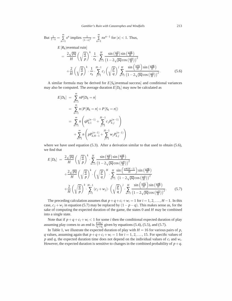
In Table 1, we illustrate the expected duration of play withH = 16 for various pairs ofp,q values, assuming again thatp+q+ci +wi = 1 for i = 1, 2, . . . , 15. For specific values ofp andq, the expected duration time does not depend on the individual values ofci andwi .However, the expected duration is sensitive to changes in the combined probability ofp+q.
214 B. Hunter, A.C. Krinik, C. Nguyen, J.M. Switkes & H.F. von Bremen
Table 1. Expected duration of playDk with H = 16 for several pairs ofp, q valueswith p+q+ci +wi = 1 for i = 1, 2, . . . , 15. For fixedp andq, the expected durationtime does not depend on the individual values ofci andwi
k p=0.5, q=0.5 p=0.45, q=0.45 p=0.3, q=0.6 p=0.2, q=0.4
0 0 0 0 0
1 15 3.73 2.152 1.4039
2 28 6.06 3.842 2.0194
3 39 7.52 5.167 2.2893
4 48 8.42 6.207 2.4076
5 55 8.97 7.024 2.4595
6 60 9.30 7.664 2.4822
7 63 9.47 8.165 2.4922
8 64 9.52 8.556 2.4966
9 63 9.47 8.857 2.4984
10 60 9.30 9.079 2.4991
11 55 8.97 9.214 2.4984
12 48 8.42 9.222 2.4941
13 39 7.52 8.980 2.4736
14 28 6.06 8.156 2.3798
15 15 3.73 5.894 1.9519
16 0 0 0 0
6. Infinite-time ruin probabilities with all probabilities variable
Assume now that all probabilities are state-dependent as inFigure 7, withpi +qi +ci +wi = 1, for i = 1, 2, . . . ,H −1. The system of difference equations in (2.1) now looks like
r0 = 1r1 = c1 +q1r0 + p1r2
r2 = c2 +q2r1 + p2r3...
rk = ck +qkrk−1 + pkrk+1 (6.1)...
rH−1 = cH−1 +qH−1rH−2 + pH−1rH
rH = 0.
Sincec1 andq1 are both probabilities from state 1 to state 0, we will without loss of gener-ality setq1 = 0. That is, in what follows one may replacec1 with c1 + q1 if one wishes toexhibit explicitly both these probabilities. Solving forrk, k = 2, 3, . . . ,H−1, in terms ofr1,the first few results are
r2 =1p1
[r1−c1]
r3 =1
p1p2[(1− p1q2) r1− (c1 + p1c2)]
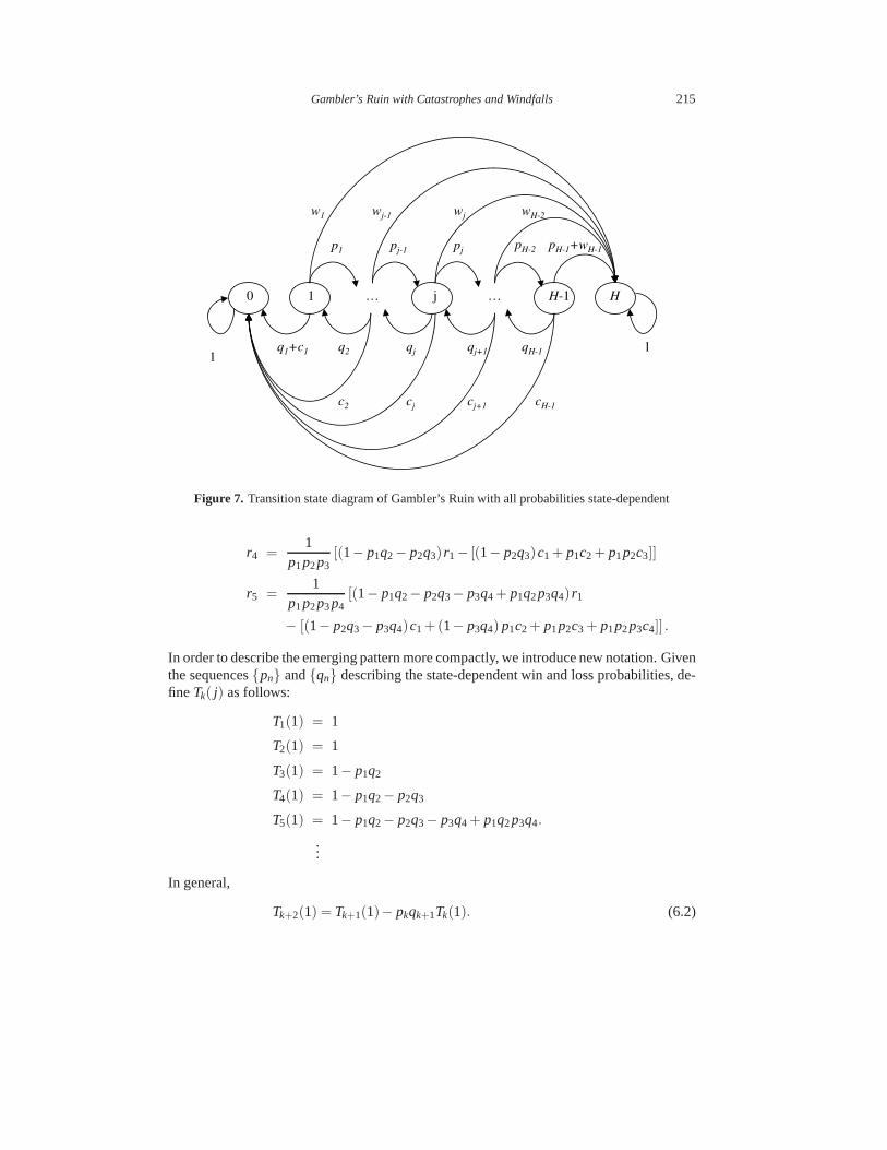
Gambler’s Ruin with Catastrophes and Windfalls 215
q1+c1
0 1 j… … HH-1
q2
p1
11
w1 wj-1 wj wH-2
pH-1+wH-1
c2 cj cj+1 cH-1
pj-1 pj
qj qj+1 qH-1
pH-2
Figure 7. Transition state diagram of Gambler’s Ruin with all probabilities state-dependent
r4 =1
p1p2p3[(1− p1q2− p2q3) r1− [(1− p2q3)c1 + p1c2 + p1p2c3]]
r5 =1
p1p2p3p4[(1− p1q2− p2q3− p3q4 + p1q2p3q4) r1
− [(1− p2q3− p3q4)c1 +(1− p3q4) p1c2 + p1p2c3 + p1p2p3c4]] .
In order to describe the emerging pattern more compactly, weintroduce new notation. Giventhe sequences{pn} and{qn} describing the state-dependent win and loss probabilities, de-fine Tk( j) as follows:
T1(1) = 1
T2(1) = 1
T3(1) = 1− p1q2
T4(1) = 1− p1q2− p2q3
T5(1) = 1− p1q2− p2q3− p3q4 + p1q2p3q4.
...
In general,
Tk+2(1) = Tk+1(1)− pkqk+1Tk(1). (6.2)
216 B. Hunter, A.C. Krinik, C. Nguyen, J.M. Switkes & H.F. von Bremen
The argumentj of Tk( j) will describe the starting subscript in the win probabilities appear-ing in Tk( j), k > 2. That is, fork = 3,
T3(1) = 1− p1q2
T3(2) = 1− p2q3
T3(3) = 1− p3q4
...
T3( j) = 1− p jq j+1.
The recursion relation (6.2) becomes
Tk+2( j) = Tk+1( j)− pk+ j−1qk+ jTk( j).
with
T1( j) = T2( j) = 1, for all j > 0.
With this notation,
rk =1
p1p2 · · · pk−1
[
Tk(1)r1−k−1
∑i=1
Ti(k− i +1)p0p1p2 · · · pk−(i+1)ck−i
]
(6.3)
follows inductively where we definep0 = 1 for notational convenience.
From (6.1), usingrH = 0,
rH−1 = cH−1 +qH−1rH−2. (6.4)
Using (6.3) to substitute into (6.4) forrH−1 andrH−2, and solving forr1, we obtain
r1 =
[
H−2∑
i=1Ti(H − i)p0p1 · · · pH−i−2cH−i−1
]
+ p1p2 · · · pH−2cH−1
TH−1(1)− pH−2qH−1TH−2(1)
−
[
qH−1pH−2
H−3∑
i=1Ti(H − i −1)p0p1 · · · pH−i−3cH−i−2
]
TH−1(1)− pH−2qH−1TH−2(1)(6.5)
=
H−3∑
i=1[Ti+1(H − i −1)− pH−2qH−1Ti(H − i −1)] · [p0p1 · · · pH−i−3cH−i−2]
TH(1)
+p1p2 · · · pH−3 [pH−2cH−1 +cH−2]
TH(1)(6.6)
where we again recall that for notational convenience we have combined the effects ofc1
andq1 by assumingq1 = 0; c1 can be replaced byc1 + q1 in order to keep the two effectsseparate. Substituting this formula into (6.3) gives an expression forrk, k = 1, 2, . . . ,H−1.
Gambler’s Ruin with Catastrophes and Windfalls 217
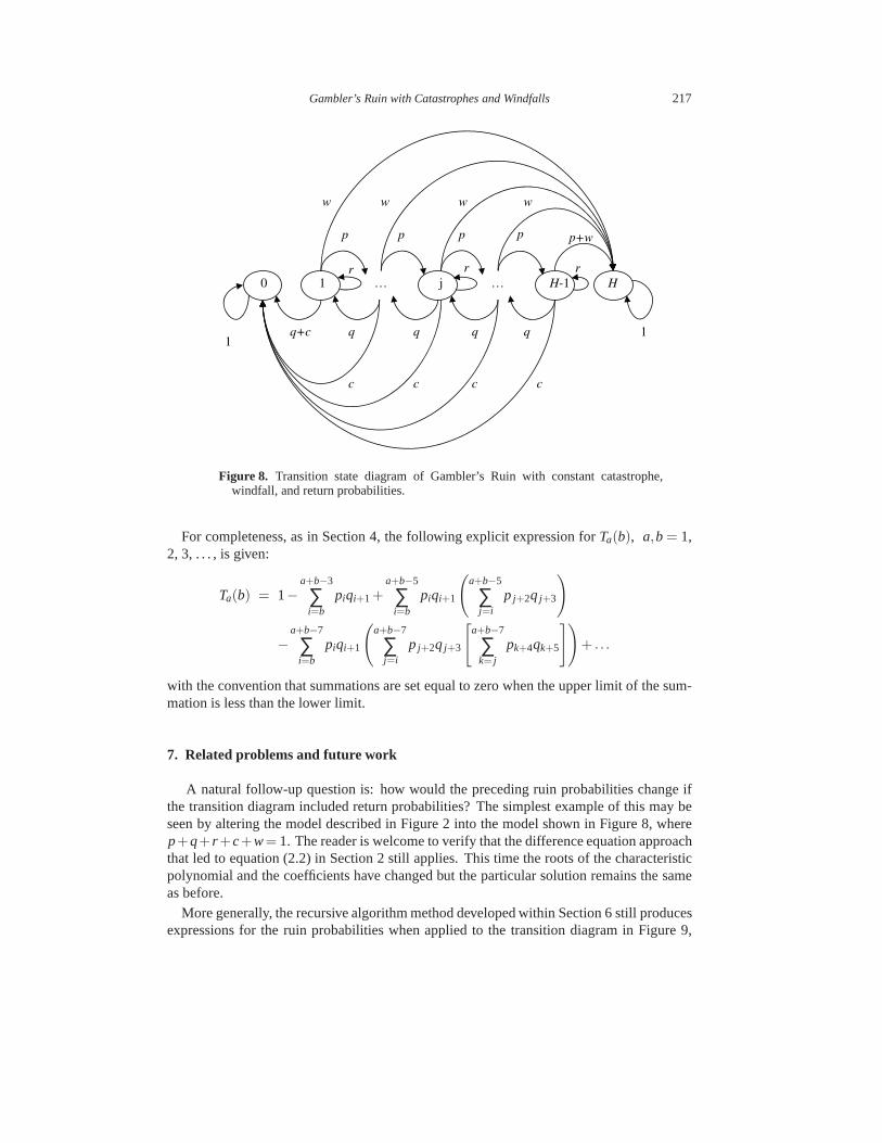
q+c
0 1 j… … HH-1
q
p
11
w w w w
p+w
c c c c
p p
q q q
p
rrr
Figure 8. Transition state diagram of Gambler’s Ruin with constant catastrophe,windfall, and return probabilities.
For completeness, as in Section 4, the following explicit expression forTa(b), a,b = 1,2, 3, . . . , is given:
Ta(b) = 1−a+b−3
∑i=b
piqi+1+a+b−5
∑i=b
piqi+1
(
a+b−5
∑j=i
p j+2q j+3
)
−a+b−7
∑i=b
piqi+1
(
a+b−7
∑j=i
p j+2q j+3
[
a+b−7
∑k= j
pk+4qk+5
])
+ . . .
with the convention that summations are set equal to zero when the upper limit of the sum-mation is less than the lower limit.
7. Related problems and future work
A natural follow-up question is: how would the preceding ruin probabilities change ifthe transition diagram included return probabilities? Thesimplest example of this may beseen by altering the model described in Figure 2 into the model shown in Figure 8, wherep+q+ r +c+w= 1. The reader is welcome to verify that the difference equation approachthat led to equation (2.2) in Section 2 still applies. This time the roots of the characteristicpolynomial and the coefficients have changed but the particular solution remains the sameas before.
More generally, the recursive algorithm method developed within Section 6 still producesexpressions for the ruin probabilities when applied to the transition diagram in Figure 9,
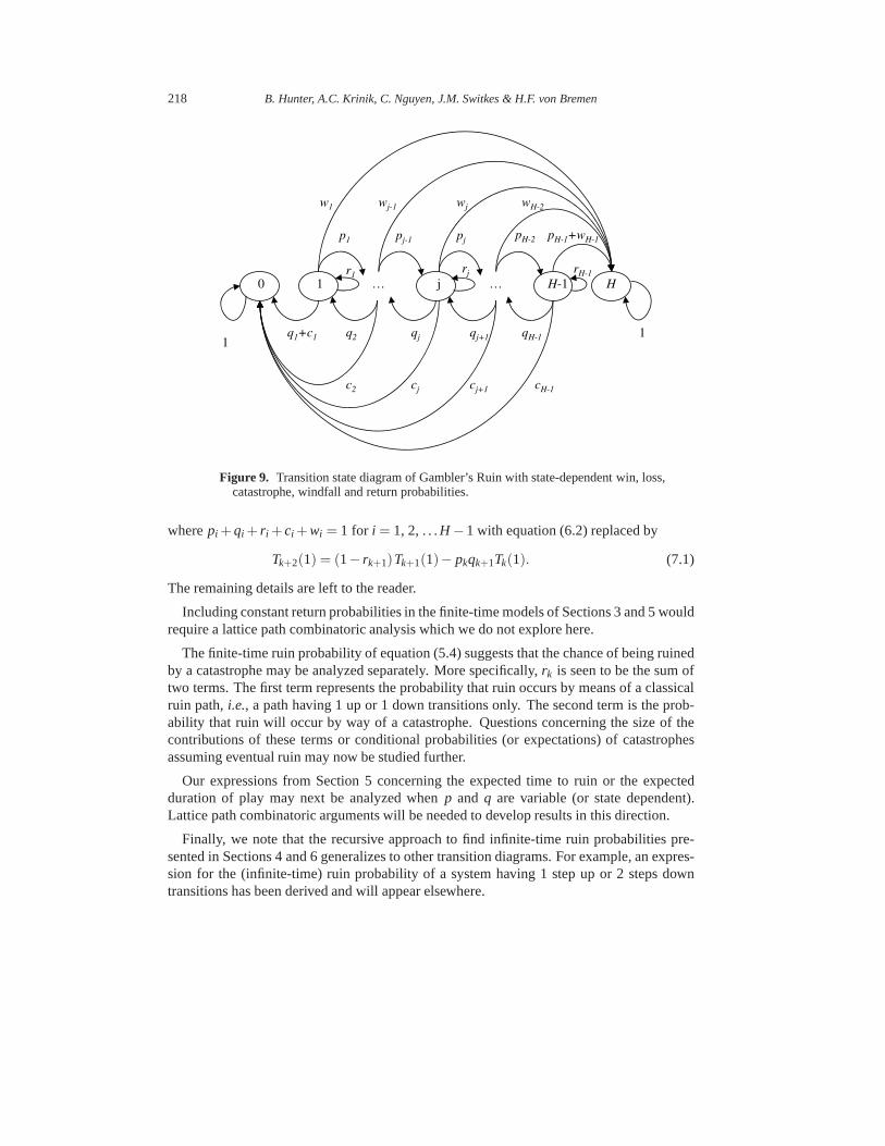
218 B. Hunter, A.C. Krinik, C. Nguyen, J.M. Switkes & H.F. von Bremen
q1+c1
0 1 j… … HH-1
q2
p1
11
w1 wj-1 wj wH-2
pH-1+wH-1
c2 cj cj+1 cH-1
pj-1 pj
qj qj+1 qH-1
pH-2
rH-1rjr1
Figure 9. Transition state diagram of Gambler’s Ruin with state-dependent win, loss,catastrophe, windfall and return probabilities.
wherepi +qi + r i +ci +wi = 1 for i = 1, 2, . . .H −1 with equation (6.2) replaced by
Tk+2(1) = (1− rk+1)Tk+1(1)− pkqk+1Tk(1). (7.1)
The remaining details are left to the reader.
Including constant return probabilities in the finite-timemodels of Sections 3 and 5 wouldrequire a lattice path combinatoric analysis which we do notexplore here.
The finite-time ruin probability of equation (5.4) suggeststhat the chance of being ruinedby a catastrophe may be analyzed separately. More specifically, rk is seen to be the sum oftwo terms. The first term represents the probability that ruin occurs by means of a classicalruin path,i.e., a path having 1 up or 1 down transitions only. The second termis the prob-ability that ruin will occur by way of a catastrophe. Questions concerning the size of thecontributions of these terms or conditional probabilities(or expectations) of catastrophesassuming eventual ruin may now be studied further.
Our expressions from Section 5 concerning the expected timeto ruin or the expectedduration of play may next be analyzed whenp and q are variable (or state dependent).Lattice path combinatoric arguments will be needed to develop results in this direction.
Finally, we note that the recursive approach to find infinite-time ruin probabilities pre-sented in Sections 4 and 6 generalizes to other transition diagrams. For example, an expres-sion for the (infinite-time) ruin probability of a system having 1 step up or 2 steps downtransitions has been derived and will appear elsewhere.
Gambler’s Ruin with Catastrophes and Windfalls 219
8. Conclusion
The main results in this article consist of recursive approaches to compute ruin probabil-ities in a variety of Gambler’s Ruin problems which have beengeneralized to include catas-trophe and windfall probabilities as well as the traditional win and loss probabilities. Ruinprobabilities of these systems, in both infinite-time and finite-time, have been obtained usingdifferent methods of solution including difference equations, lattice path combinatorics andpattern recognition. Numerical examples illustrating these ruin probabilities are presented.Solutions to questions concerning the expected duration ofplay and the expected time toruin (conditioned upon the assumption that ruin will occur)have been developed along theway. Some of the recursive methods are robust and provide ruin probability solutions foreven more generalized types of transition diagrams.
References
Ash, R. B., 1970.Basic Probability Theory, John Wiley and Sons, Inc., New York.Edwards, A. W. F., 1983. Pascal’s problem: the “Gambler’s Ruin”. International Statistical Review, 73–79.Feller, W., 1968.An Introduction to Probability Theory and its Applications, Volume 1, 3rd edition, John
Wiley and Sons, Inc., New York.Goldberg, S., 1986.Introduction to Difference Equations, with Illustrative Examples from Economics, Psy-
chology, and Sociology, Dover Publications, Inc., New York.Harper, J. D., Ross, K. A., 2005. Stopping strategies and Gambler’s ruin.Mathematics Magazine, 255–268.Hoel, P., Port, S., Stone, C., 1987.Introduction to Stochastic Processes, Waveland Press Inc.Hunter, B., 2005.Gambler’s Ruin and the Three State Process, Master’s Thesis, California State Polytechnic
University, Pomona.Krinik, A., Rubino, G., Marcus, D., Swift, R., Kasfy, H., Lam, H., 2005. Dual processes to solve single
serve systems.Journal of Statistical Planning and Inference Special Issue on Lattice Path Combinatoricsand Discrete Distributions135, 121–147.
Marcus, D., 1998.Combinatorics: A Problem Oriented Approach, The Mathematical Association of Amer-ica, Washington.
Mohanty, S. G., 1979.Lattice Path Counting and Applications, Academic Press.Narayana, T. V., 1979.Lattice Path Combinatorics With Statistical Applications, University of Toronto
Press, Toronto.Takacs, L., 1969. On the Classical Ruin Problems.American Statistical Association Journal64, 889–906.


![Gambler’s Ruin Bandit Problem · A. Gambler’s Ruin Problem If action F is removed from the GRBP, it becomes the Gambler’s Ruin Problem. In the model of Hunter et al. [10] of](https://img.pdfslide.net/doc/110x75/5f0c18f57e708231d433ba74/gambleras-ruin-bandit-problem-a-gambleras-ruin-problem-if-action-f-is-removed.jpg)