Gas Price Spikes.1

8/7/2019 Gas Price Spikes.1

http://slidepdf.com/reader/full/gas-price-spikes1 1/28

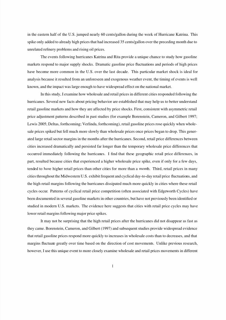
Temporary Wholesale Gasoline Price Spikes have Long-lastingRetail Effects: The Aftermath of Hurricane Rita

Matthew S. Lewis The Ohio State University

Abstract

I study U.S. gasoline prices following Hurricane Rita to show that short-lived geographical differences

in the severity of wholesale gasoline price spikes are associated with long-lasting geographical differ-

ences in retail prices. In most U.S. cities, wholesale prices spiked significantly for roughly two weeks

following the hurricane. However, in cities where this spike was particularly large, retail margins re-

mained higher than in other cities for nearly two months. High retail margins dissipated more quickly

after the hurricane in cities where competition between stations tends to generate cyclical retail price

fluctuations independent of wholesale cost movements. I discuss why prices may have fallen faster in

cities exhibiting retail price cycles and present additional results identifying differences in market char-

acteristics between cities with and without price cycles. I find that cycling cities tend to have higher

population density and have independent (non-refinery brand) stations that are more highly concentrated

into large retail chains.

1. Introduction

The summer of 2005 was a particularly bad hurricane season for the Gulf of Mexico region. Two

severely destructive hurricanes, Katrina and Rita, hit within one month of each other in August and Septem-

ber. Though the heaviest losses occurred in the Gulf region, one of the most immediate and well publicized

impacts of the hurricanes on the rest of the U.S. was their effect on gasoline prices and other energy mar-

kets. Most of the oil extraction, transportation and refining facilities concentrated in the Gulf region were

either damaged or temporarily closed during the storms, causing major disruption in the nation’s supply of

petroleum products.1 Much of the South, East Coast, and Midwest are dependent on both crude oil and

refined gasoline produced in or imported through the Gulf region. As a result, average retail gasoline prices

I am grateful to Sam Peltzman, an anonymous coeditor, and an anonymous referee for detailed comments and suggestions.I also benefited greatly from the comments of Severin Borenstein, Trevon Logan, Preston McAfee, Erich Muehlegger and of

seminar participants at The Ohio State University, Kent State University, the Federal Trade Commission, the 2008 International

Industrial Organization Conference, and the University of California’s Center for the Study of Energy Markets’ Oil and Gasoline

Research Conference.1Nearly all of the oil production and refining in the Gulf region stopped for one to two weeks during Hurricane Rita. Half of

the refining capacity and two-thirds of the oil production capacity in the area remained down for over a month. The Gulf region

accounts for over 50% of domestic crude oil production capacity and around 33% of domestic refining capacity. See Hibbard

(2006).

Forthcoming in The Journal of Law and Economics, Volume 52 Draft date: June 2008



in the eastern half of the U.S. jumped nearly 60 cents/gallon during the week of Hurricane Katrina. This

spike only added to already high prices that had increased 35 cents/gallon over the preceding month due to

unrelated refinery problems and rising oil prices.

The events following hurricanes Katrina and Rita provide a unique chance to study how gasoline

markets respond to major supply shocks. Dramatic gasoline price fluctuations and periods of high prices

have become more common in the U.S. over the last decade. This particular market shock is ideal for

analysis because it resulted from an unforeseen and exogenous weather event, the timing of events is well

known, and the impact was large enough to have widespread effect on the national market.

In this study, I examine how wholesale and retail prices in different cities responded following the

hurricanes. Several new facts about pricing behavior are established that may help us to better understand

retail gasoline markets and how they are affected by price shocks. First, consistent with asymmetric retail

price adjustment patterns described in past studies (for example Borenstein, Cameron, and Gilbert 1997;

Lewis 2005; Deltas, forthcoming; Verlinda, forthcoming), retail gasoline prices rose quickly when whole-

sale prices spiked but fell much more slowly than wholesale prices once prices began to drop. This gener-

ated large retail sector margins in the months after the hurricanes. Second, retail price differences between

cities increased dramatically and persisted far longer than the temporary wholesale price differences that

occurred immediately following the hurricanes. I find that these geographic retail price differences, in

part, resulted because cities that experienced a higher wholesale price spike, even if only for a few days,

tended to have higher retail prices than other cities for more than a month. Third, retail prices in many

cities throughout the Midwestern U.S. exhibit frequent and cyclical day-to-day retail price fluctuations, and

the high retail margins following the hurricanes dissipated much more quickly in cities where these retail

cycles occur. Patterns of cyclical retail price competition (often associated with Edgeworth Cycles) have

been documented in several gasoline markets in other countries, but have not previously been identified or

studied in modern U.S. markets. The evidence here suggests that cities with retail price cycles may have

lower retail margins following major price spikes.

It may not be surprising that the high retail prices after the hurricanes did not disappear as fast as

they came. Borenstein, Cameron, and Gilbert (1997) and subsequent studies provide widespread evidence

that retail gasoline prices respond more quickly to increases in wholesale costs than to decreases, and that

margins fluctuate greatly over time based on the direction of cost movements. Unlike previous research,

however, I use this unique event to more closely examine wholesale and retail prices movements in different

1



cities following a large price spike. Relatively little is known about why geographic differences in retail

gasoline margins arise and how they fluctuate over time. The patterns uncovered here reveal several market

factors that help to explain how differences in margins arise in association with large market shocks.

The identification of cyclical retail price competition in some Midwestern U.S. cities is also signifi-

cant. Though the fairly recent availability of daily price data has made the discovery and study of these high

frequency cyclical pricing patterns possible, anecdotal sources suggest that these price cycles have occurred

in the region for many years. I use the hurricanes to compare how retail margins respond to market shocks

in cities with and without cyclical price competition. Large and significant differences in margins arise

between cycling and non-cycling cities after the hurricanes, representing a major source of the increased

geographic variation in margins observed during the period.

Very little is know about what generates cyclical retail price competition in some gasoline markets

but not others. As a result, I attempt to identify differences in market characteristics between cycling and

non-cycling cities in my sample. Using information on brand market shares within each city, I find that

cities in which independent (non-refinery brand) stations are concentrated into larger retail brands or chains

(such as QuikTrip, Speedway, or Kroger) are more likely to exhibit retail price cycles than cities where

independent stations tend to be run on a smaller scale. This new finding suggests that the presence of

large independent retail operations may influence the tendency for aggressive price cutting or the ability to

coordinate market wide price increases, which are necessary for cycles to occur.

Understanding regional variation in retail margins, particularly surrounding large price spikes, is

of considerable interest given the heightened sensitivity of the public and of policymakers toward potential

signs of anticompetitive behavior. Large differences in margins also suggest the possibility of efficiency

losses due to imperfect competition or market frictions. Following a Congressional mandate, the Federal

Trade Commission investigated the effects of the hurricanes on gasoline prices and of the possibility for

price manipulation.2 The FTC report describes geographic differences in the size of the resulting price

spikes, and concludes that most of the retail price differences were driven by wholesale prices. However, the

report does not analyze the geographic differences in retail margins and the speed with which retail prices

fell over the following months, or how this may have been related to the local competitive environment.

The properties of regional variation in margins that I present here should help in beginning to construct a

more complete picture of overall retail gasoline market performance and the appropriateness of potential

2U.S. Federal Trade Commission (2006) is a written account of the results of this investigation.

2



government action. Furthermore, since very little is known about the relative competitiveness of markets

exhibiting retail price cycles, comparisons of market outcomes and market characteristics between cycling

and non-cycling markets provide an important initial contribution to inform future research.

In the next two sections of the paper I describe the data being used and discuss geographic differ-

ences in retail and wholesale gasoline prices following Hurricanes Katrina and Rita. Section 3 also includes

several illustrative examples comparing price movements in cities with and without retail price cycles, and

in cities that differ in the severity of their hurricane related wholesale price spike. Section 4 presents the for-

mal empirical investigation of how post-Rita retail prices relate to the severity of wholesale shock and the

presence of retail cycles. Given the large differences in post-hurricane pricing between cycling and non-

cycling cities, Section 5 adds some exploratory analysis identifying differences in market characteristics

and competitive structure between cities with and without cycles. Section 6 concludes.

2. Data

Daily retail and wholesale gasoline prices are observed for 85 cities throughout the Midwest, Mid-

Atlantic, and Southern states. The sample was chosen to represent a relatively complete collection of major

cities within this contiguous geographic area.3 Retail and wholesale price data are provided by Oil Price

Information Service (OPIS). Retail prices are average prices from samples of stations within each city and

are reported with all relevant taxes removed.4 Wholesale prices are observed at local distribution racks.

These are facilities located near the city where gasoline is drawn out of a pipeline and loaded onto tanker-

trucks for transport to local gas stations. The rack price for unbranded gasoline is used as the wholesale

price for each city because it represents the true local marginal cost of the homogeneous commodity coming

off the pipeline. This unbranded gasoline is then sold by local unbranded stations, or is combined with the

additives of a major gasoline brand (such as BP, Shell, or Chevron) and marked up for sale to that company’s

own branded station operators.

3. Geographic Differences in Response to Market Shocks

Figure 1 shows the daily average retail and wholesale prices across the 85 cities observed during

3Daily wholesale and retail price surveys were collected by Oil Price Information Service and are observed for all of 2004 and

2005. States with cities in the sample include: AL, AR, GA, IA, IL, IN, KS, KY, MI, MN, MO, NC, NE, NY, OH, OK, PA, TN,

TX, WI, WV.4The price collected from each station is for unleaded 87-octane gasoline.

3



$1.40

$1.60

$1.80

$2.00

$2.20

$2.40

$2.60

$2.80Average Wholesale Price

Average Retial Price

$-

$0.04

$0.08

$0.12

$0.16

$0.20

2 2 - J u n

- 0 5

6 - J u l - 0

5

2 0 - J u l -

0 5

3 - A u

g - 0 5

1 7 - A u g

- 0 5

3 1 - A u g

- 0 5

1 4 - S e p

- 0 5

2 8 - S e p

- 0 5

1 2 - O c t -

0 5

2 6 - O c t -

0 5

9 - N o

v - 0 5

2 3 - N o v - 0 5

7 - D e

c - 0 5

2 1 - D e c

- 0 5

Standard Deviation of Wholesale

Standard Deviation of Retail

HurricaneKatrina

HurricaneRita$/Gallon

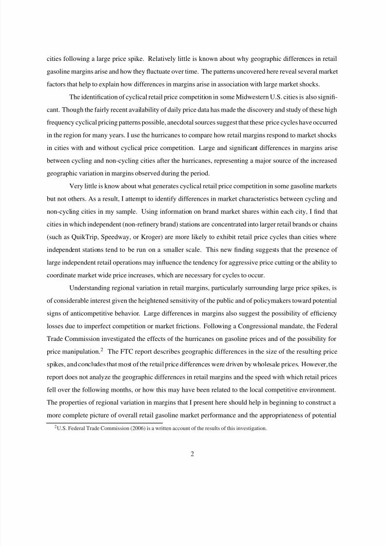
Figure 1. Means and Standard Deviations of Daily Gasoline Prices Across Cities.

the time period surrounding the hurricanes. It also shows the standard deviation in the observed prices

across cities in the sample. The average retail and wholesale price series reveal the large price increases

that occurred in response to the two hurricanes, as well as the gradual increase in prices in July and August

resulting from rising oil prices and a number of unrelated U.S. refinery outages. However, after the hurri-

canes, wholesale prices increased much more in some cities than in others. Spikes in the standard deviation

of wholesale prices in Figure 1 reveal large geographic differences immediately following the hurricanes.

For example, after Hurricane Rita wholesale gasoline prices topped out at $2.92 per gallon in Charlotte, NC

(the highest in the sample) and $2.27 per gallon in Syracuse, NY (the lowest in the sample). These price

differences arose because certain regions are more dependant on gasoline produced at Gulf Coast refineries

or on crude oil and gasoline transported using pipelines or ports affected by the hurricanes. 5 In the days

following each disruption, adjustments were made within the supply network to mitigate the regional price

differences, and the standard deviation of wholesale prices decreases fairly quickly towards more normal

levels. Interestingly, regional differences in retail prices grew larger well after regional wholesale price

differences had returned to normal.

5Regions such as the Upper Midwest and Northeast have some refining capacity of their own and have access to imported oil

and/or refined products from Canada or elsewhere (through marine terminals in the Great Lakes and New England). Price spikes

in these areas tended to be smaller.

4



$1.20

$1.40

$1.60

$1.80

$2.00

$2.20

$2.40

$2.60

$2.80

$3.00

1 1 - S e p

- 0 5

1 8 - S e p

- 0 5

2 5 - S e p

- 0 5

2 - O c t - 0 5

9 - O c t - 0 5

1 6 - O c t - 0 5

2 3 - O c t - 0 5

3 0 - O c t - 0 5

6 - N o

v - 0 5

1 3 - N o v - 0 5

2 0 - N o v - 0 5

2 7 - N o v - 0 5

4 - D e

c - 0 5

1 1 - D e c

- 0 5

1 8 - D e c

- 0 5

2 5 - D e c

- 0 5

Pittsburgh Retail

Pittsburgh Wholesale

Nashville Retail

Nashville Wholesale

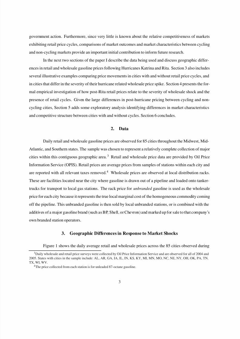
Figure 2. Prices in Nashville and Pittsburgh Before and After Hurricane Rita.

3.1. Importance of the Local Peak Wholesale Prices

Geographic differences in the severity of the local wholesale shock appear to be a contributing

factor in persistent dispersion of retail prices following the spike. In cities that faced relatively high whole-

sale prices during the disruption, retail prices and retail margins remained much higher than in other areas

for several months. An example is illustrated in Figure 2. Retail prices in Nashville increased more than

in Pittsburgh because Nashville experienced a larger wholesale price spike (roughly 43 cents per gallon

higher) following the hurricane. However, retail prices (and margins) remained higher in Nashville long

after the wholesale price had fallen close to the levels seen in Pittsburgh. The persistent difference in retail

margins appears to be economically significant. One month after Rita, wholesale prices in Pittsburgh and

Nashville were fluctuating within a few cents of each other while retail prices in Nashville were still 30

cents higher. The empirical analysis in Section 4 attempts to more systematically examine whether tempo-

rary geographic differences in wholesale prices between cities are associated with large and fairly persistent

geographic differences in retail prices.

3.2. Importance of the Local Competitive Environment

Geographic retail price dispersion may have also arisen due to differences in the way that gas

stations compete within each city. Retail prices fell more quickly after the hurricanes in regions that exhibit

5



$1.00

$1.10

$1.20

$1.30

$1.40

$1.50

$1.60

$1.70

$1.80

1 0 - M a y

- 0 4

2 4 - M a y

- 0 4

7 - J u n - 0 4

2 1 - J u n - 0 4

5 - J u l - 0

4

1 9 - J u l - 0

4

2 - A u

g - 0 4

1 6 - A u g

- 0 4

3 0 - A u g

- 0 4

1 3 - S e p

- 0 4

2 7 - S e p

- 0 4

Pittsburgh Retail

Pittsburgh Wholesale

Columbus Retail

Columbus Wholesale

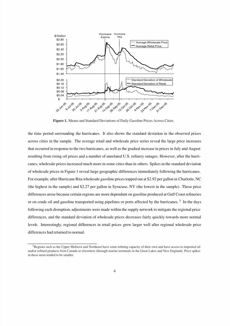
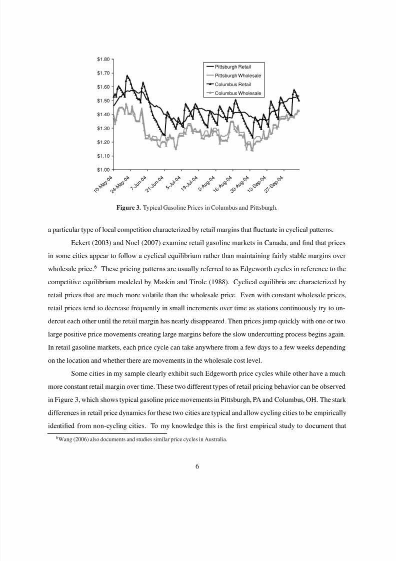
Figure 3. Typical Gasoline Prices in Columbus and Pittsburgh.

a particular type of local competition characterized by retail margins that fluctuate in cyclical patterns.

Eckert (2003) and Noel (2007) examine retail gasoline markets in Canada, and find that prices

in some cities appear to follow a cyclical equilibrium rather than maintaining fairly stable margins over

wholesale price.6 These pricing patterns are usually referred to as Edgeworth cycles in reference to the

competitive equilibrium modeled by Maskin and Tirole (1988). Cyclical equilibria are characterized by

retail prices that are much more volatile than the wholesale price. Even with constant wholesale prices,

retail prices tend to decrease frequently in small increments over time as stations continuously try to un-

dercut each other until the retail margin has nearly disappeared. Then prices jump quickly with one or two

large positive price movements creating large margins before the slow undercutting process begins again.

In retail gasoline markets, each price cycle can take anywhere from a few days to a few weeks depending

on the location and whether there are movements in the wholesale cost level.

Some cities in my sample clearly exhibit such Edgeworth price cycles while other have a much

more constant retail margin over time. These two different types of retail pricing behavior can be observed

in Figure 3, which shows typical gasoline price movements in Pittsburgh, PA and Columbus, OH. The stark

differences in retail price dynamics for these two cities are typical and allow cycling cities to be empirically

identified from non-cycling cities. To my knowledge this is the first empirical study to document that

6Wang (2006) also documents and studies similar price cycles in Australia.

6



$1.20

$1.40

$1.60

$1.80

$2.00

$2.20

$2.40

$2.60

2 9 - S e p

- 0 5

0 6 - O c t -

0 5

1 3 - O c t -

0 5

2 0 - O c t -

0 5

2 7 - O c t -

0 5

0 3 - N o v - 0 5

1 0 - N o v - 0 5

1 7 - N o v - 0 5

2 4 - N o v - 0 5

0 1 - D e c

- 0 5

0 8 - D e c

- 0 5

1 5 - D e c

- 0 5

2 2 - D e c

- 0 5

2 9 - D e c

- 0 5

Philadelphia Retail

Philadelphia Wholesale

Columbus Retail

Columbus Wholesale

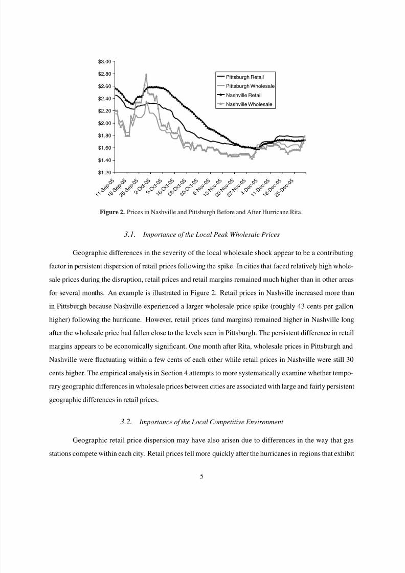
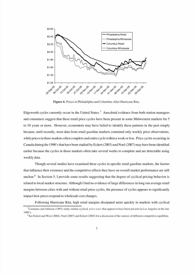
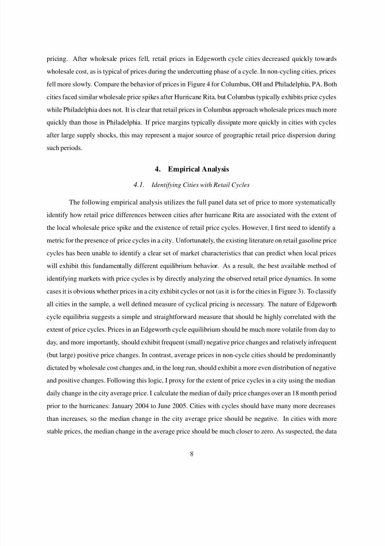
Figure 4. Prices in Philadelphia and Columbus After Hurricane Rita.

Edgeworth cycles currently occur in the United States.7 Anecdotal evidence from both station managers

and consumers suggest that these retail price cycles have been present in some Midwestern markets for 5

to 10 years or more. However, economists may have failed to identify these patterns in the past simply

because, until recently, most data from retail gasoline markets contained only weekly price observations,

while prices in these markets often complete and entire cycle within a week or less. Price cycles occurring in

Canada during the 1990’s that have been studied by Eckert (2003) and Noel (2007) may have been identified

earlier because the cycles in those markets often take several weeks to complete and are detectable using

weekly data.

Though several studies have examined these cycles in specific retail gasoline markets, the factors

that influence their existence and the competitive effects they have on overall market performance are still

unclear.8 In Section 5, I provide some results suggesting that the degree of cyclical pricing behavior is

related to local market structure. Although I find no evidence of large differences in long run average retail

margins between cities with and without retail price cycles, the presence of cycles appears to significantly

impact how prices respond to wholesale cost changes.

Following Hurricane Rita, high retail margins dissipated more quickly in markets with cyclical

7Castanias and Johnson (1993) study similar cyclical price wars that appear to have been present in Los Angeles in the late

1960’s.8See Eckert and West (2004), Noel (2007) and Eckert (2003) for a discussion of the sources of different competitive equilibria.

7



pricing. After wholesale prices fell, retail prices in Edgeworth cycle cities decreased quickly towards

wholesale cost, as is typical of prices during the undercutting phase of a cycle. In non-cycling cities, prices

fell more slowly. Compare the behavior of prices in Figure 4 for Columbus, OH and Philadelphia, PA. Both

cities faced similar wholesale price spikes after Hurricane Rita, but Columbus typically exhibits price cycles

while Philadelphia does not. It is clear that retail prices in Columbus approach wholesale prices much more

quickly than those in Philadelphia. If price margins typically dissipate more quickly in cities with cycles

after large supply shocks, this may represent a major source of geographic retail price dispersion during

such periods.

4. Empirical Analysis

4.1. Identifying Cities with Retail Cycles

The following empirical analysis utilizes the full panel data set of price to more systematically

identify how retail price differences between cities after hurricane Rita are associated with the extent of

the local wholesale price spike and the existence of retail price cycles. However, I first need to identify a

metric for the presence of price cycles in a city. Unfortunately, the existing literature on retail gasoline price

cycles has been unable to identify a clear set of market characteristics that can predict when local prices

will exhibit this fundamentally different equilibrium behavior. As a result, the best available method of

identifying markets with price cycles is by directly analyzing the observed retail price dynamics. In some

cases it is obvious whether prices in a city exhibit cycles or not (as it is for the cities in Figure 3). To classify

all cities in the sample, a well defined measure of cyclical pricing is necessary. The nature of Edgeworth

cycle equilibria suggests a simple and straightforward measure that should be highly correlated with the

extent of price cycles. Prices in an Edgeworth cycle equilibrium should be much more volatile from day to

day, and more importantly, should exhibit frequent (small) negative price changes and relatively infrequent

(but large) positive price changes. In contrast, average prices in non-cycle cities should be predominantly

dictated by wholesale cost changes and, in the long run, should exhibit a more even distribution of negative

and positive changes. Following this logic, I proxy for the extent of price cycles in a city using the mediandaily change in the city average price. I calculate the median of daily price changes over an 18 month period

prior to the hurricanes: January 2004 to June 2005. Cities with cycles should have many more decreases

than increases, so the median change in the city average price should be negative. In cities with more

stable prices, the median change in the average price should be much closer to zero. As suspected, the data

8



reveal two types of cities: those with median price changes massed around zero and those with negative

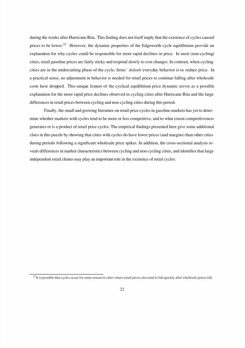
and sizable median price changes. More specifically, 45% of observed cities have a median price change

between -.1 and .1 cents per gallon (the maximum for the sample), while 55% have median price changes

from -.1 to -1.5 cents per gallon. Appendix Figure A1 shows a kernel density plot of the distribution of

median price changes for the cities observed.

While a negative median price change measure should identify cities with cyclical pricing behavior,

one might also be concerned that this measure may simply be capturing non-cycling cities that exhibit

highly asymmetric price adjustment or cities that simply have more wholesale price volatility. If retail prices

in a city tend to respond very quickly when wholesale prices increase and very slowly when wholesale

prices decrease, this will most likely cause the median daily price change to be more negative. Similarly, if

wholesale costs are less volatile in some cities, the median price change may be closer to zero in these cities

because prices are not (asymmetrically) adjusting to as many cost changes. I argue, however, that highly

asymmetric adjustment to cost changes has a much smaller effect on the median price change measure than

would the existence of retail price cycles.

Cities with cycles tend to have more retail price movements in general and more frequent positive

price jumps since prices often jump even without a significant increase in wholesale cost. To confirm my

interpretation of the median price change measure I compare the number of significant jumps in retail price

and wholesale cost across cities during the pre-hurricane period. I define a price (or cost) jump as an event

in which prices increase by 4 cents per gallon or more in one day or over two consecutive days.9 Wholesale

costs across cities usually move together, so it is not surprising that 90% of cities in the sample have between

71 and 97 wholesale price jumps from January 2004 to June 2005. Cities with lagged and asymmetric price

response would only see prices jump when costs jump, and in many cases the price response would be slow

enough to not be classified as a price jump. On the other hand, cities with retail cycles should have frequent

price jumps that often occur even in the absence of a cost increase. If both types of cities exist in the sample,

one would suspect much more variation across cities in the number of retail price jumps observed. In fact,

this is the case. Even after excluding extreme cities, the number of price jumps observed from the middle

90% of cities in the sample ranges from 13 to 157 over the 18 month period. Of the 85 cities in the sample,

35 exhibit more retail price jumps than wholesale cost jumps. Most importantly, this alternative indicator

of the presence of retail cycles is highly consistent with the median price change measure. The number

9If prices also increase in days surrounding the jump, the total price increase is still only counted as one price jump event.

9



of price jumps in the city and the median price change measure have a correlation coefficient of -.92. It

appears that there is a fundamental difference in pricing behavior across cities, that can not be explained by

varying degrees of lagged and asymmetric response to cost changes.

For the remaining empirical analysis I use the median price change measure as a metric of the

presence and severity of retail price cycling activity. While this measure is continuous, I am often interested

in discussing differences in the behavior of prices between cycling and non-cycling cities. For purposes of

interpretation, I will focus on cities with a median price change of less than -.3 cents per gallon as cycling

cities because they appear to be distinctly different from the large group of cities with a median price change

of zero (or very close to zero).10 Among the 29 cities in which the median price change is less than -.3,

the average (and median) value is roughly -.9. Therefore, when interpreting differences in the behavior of

cycling and non-cycling cities I typically compare a cycling city with a typical median price change value

of -.9 cents to a non-cycling city with a zero median price change. It is also important to note that the

presence of price cycling behavior appears to be highly persistent. There is no evidence of cycles appearing

and disappearing within a particular city during two year sample period. Furthermore, there is no indication

from more recent external data sources of any changes in the presence of cycles in the cities studied.

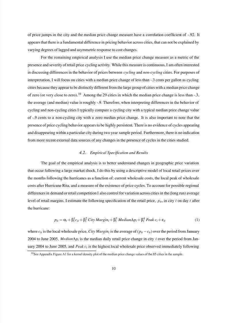
4.2. Empirical Specification and Results

The goal of the empirical analysis is to better understand changes in geographic price variation

that occur following a large market shock. I do this by using a descriptive model of local retail prices over

the months following the hurricanes as a function of: current wholesale costs, the local peak of wholesale

costs after Hurricane Rita, and a measure of the existence of price cycles. To account for possible regional

differences in demand or retail competition I also control for variation across cities in the (long run) average

level of retail margins. I estimate the following specification of the retail price, pit , in city i on day t after

the hurricane:

pit = αt +β1t cit +β2

t City Margini +β3t Median∆ pi +β4

t Peak ci + εit (1)

where cit is the local wholesale price, City Margini is the average of ( pit −cit ) over the period from January

2004 to June 2005, Median∆ pi is the median daily retail price change in city i over the period from Jan-

uary 2004 to June 2005, and Peak ci is the highest local wholesale price observed immediately following

10See Appendix Figure A1 for a kernel density plot of the median price change values of the 85 cities in the sample.

10



Hurricane Rita.11 The model is intended to describe the extent to which retail prices on a particular day

following the hurricane are correlated with the peak wholesale price or the existence of retail cycles. By al-

lowing separate coefficient values for each day I estimate how these relationships evolve over time without

the limitations of a particular functional form. The econometric model is not derived from a particular the-

ory of pricing behavior, though I discuss several possible conclusions that could be drawn from the patterns

identified. Note that since gasoline prices are highly serially correlated, the coefficients, particularly that

for Peak ci, represent the accumulated relationship between that explanatory variable and pit , including any

possible effects that feed indirectly through the retail price in previous periods.

Daily price observations are often highly serially correlated. Over short sample periods these data

can, in some cases, resemble a nonstationary process. In this case, there is a concern that the error term may

also exhibit high serial correlation causing standard error estimates to be biased downward and increasing

the possibility of a spurious regression. Since I have panel data and the model allows coefficient values

to vary across days, I take a rather conservative approach to correcting the serial correlation problem.

I effectively eliminate the time dimension by separately estimating a cross-sectional regression for each

day. While this method is possibly less efficient, it also requires no knowledge or assumptions about the

structure of correlation in prices (and errors) over time.12 The error terms (εit s) in each day’s cross-sectional

regression are certainly still correlated with those from other days, but now this correlation does not effect

the estimated standard errors for coefficient within each cross-sectional regression.13

According to the preliminary evidence from the previous section, cities experiencing larger whole-

sale price spikes during Hurricane Rita tended to have higher retail prices in the days following the hurri-

cane, and cities with retail price cycles tended to have lower retail prices following the hurricane (suggesting

that β4t > 0 & β3

t < 0). Notice that cit accounts for the contemporaneous effect of the current wholesale price

11Since the intent of the Peak ci is to measure the magnitude of the local wholesale price spike, I also consider using an

alternative measure of this magnitude: the peak wholesale price minus an historical average of the local wholesale price (from

January 2004 and June 2005) to net out any long-run geographic differences. Using this new measure instead of Peak c generates

nearly identical results to those presented below. This is not surprising given that the these two measures of the magnitude of the

local price spike have a correlation coefficient of .988. Long-run differences in average wholesale cost across cities do not appear

to significantly affect the coefficients of Equation 1.12

Several alternative procedures were performed that jointly estimate daily values of each coefficient in Equation 1 by interactingeach coefficient with a dummy variable for each day. Newey-West standard errors calculated to control for first order serial

correlation within each city were similar to, or just slightly smaller than, those reported from the daily regressions. In addition, a

Prais-Winsten regression estimating the coefficients under the assumption of an AR(1) error process resulted in very similar point

estimates and slightly smaller standard errors than those reported from the daily regressions. The alternative estimation procedures

suggest that the daily regressions are relatively efficient in this case due to a high level of serial correlation.13Correlation in error terms across daily regressions would only become important if, for example, one were to test the equality

of coefficients from different regressions.

11



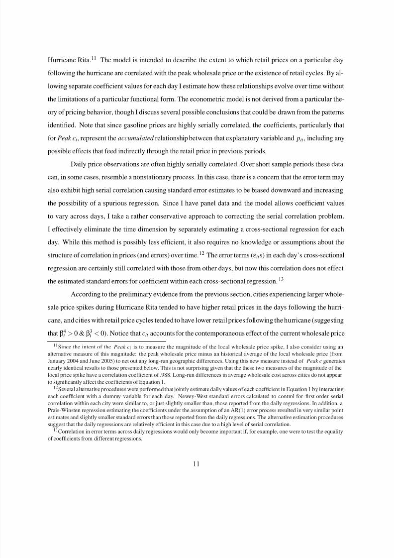
Table 1

Coefficient Estimates of Selected Daily Price Regressions from Equation 1

Date Wholesale Cost City Margin Peak c 1 Median ∆ pi constant R-squared

10/1/2005 0.165 (0.086) 1.120 (0.199) 0.337 (0.081) 1.42 (1.24) 110.4 (12.9) 0.6410/6/2005 -0.066 (0.096) 0.947 (0.173) 0.517 (0.081) 4.58 (1.53) 115.1 (14.2) 0.71

10/11/2005 0.149 (0.182) 1.173 (0.179) 0.525 (0.076) 4.38 (1.50) 56.5 (28.2) 0.69

10/16/2005 0.361 (0.163) 1.385 (0.254) 0.444 (0.063) 5.77 (1.69) 23.4 (27.1) 0.65

10/21/2005 0.241 (0.108) 1.388 (0.257) 0.433 (0.055) 8.48 (1.72) 41.7 (22.0) 0.61

10/26/2005 0.333 (0.118) 1.485 (0.286) 0.359 (0.061) 10.29 (1.71) 32.9 (23.0) 0.59

10/31/2005 0.393 (0.149) 1.554 (0.312) 0.269 (0.068) 10.26 (1.57) 38.2 (23.8) 0.55

11/5/2005 0.425 (0.156) 1.680 (0.321) 0.195 (0.067) 11.02 (1.28) 43.6 (24.6) 0.54

11/10/2005 0.451 (0.156) 1.642 (0.197) 0.101 (0.056) 2.98 (0.97) 60.9 (23.3) 0.56

11/15/2005 0.521 (0.156) 1.427 (0.219) 0.034 (0.054) 7.57 (1.00) 66.3 (23.1) 0.55

11/20/2005 0.737 (0.170) 1.274 (0.238) 0.011 (0.045) 8.79 (0.96) 38.7 (24.2) 0.61

11/25/2005 0.717 (0.188) 1.139 (0.229) -0.061 (0.039) 4.95 (1.19) 57.2 (26.5) 0.56

11/30/2005 0.965 (0.153) 1.150 (0.147) -0.014 (0.031) 0.16 (0.85) 11.9 (21.8) 0.62

Note. Regression results only reported for every fifth day. Standard errors in parenthesis.

1 Peak wholesale prices following Hurricane Rita occurred on September 29th , 2005.

on the current retail price. Therefore, the coefficient on Peak ci describes the additional correlation between

past wholesale prices and retail prices after controlling for current wholesale conditions.

14

It is interestingto note that the presence of cycles in a city appears to be completely uncorrelated with the magnitude of the

local peak wholesale price. The correlation coefficient between Peak c and Cycle is .013.

Equation 1 is estimated separately for each day using the 85 observed cities. Regression results

are displayed in Table 1, though, for brevity, only the coefficient estimates for every fifth day following

Hurricane Rita are reported. Estimation results are consistent with the preliminary analysis. Coefficient

estimates on Peak ci are positive and significant for more than a month after the price spike, with the largest

values of just over .5 coming around 10 days after the spike. This coefficient value reveals how many

cents per gallon higher the daily retail price tends to be, all else equal, for cities in which the peak of the

wholesale price spike was one cent higher. The regression controls for the current wholesale price in each

14Since retail prices tend to respond to wholesale prices with a delay, I estimate an alternative specification of the model that

includes the current wholesale price as well as several lagged wholesale price changes. This ensures that current wholesale

conditions are effectively controlled for. The results are similar to those from Equation 1 and are discussed in more detail at the

end of this section.

12



-$0.05

$0.00

$0.05

$0.10

$0.15

$0.20

$0.25

3 0 - S e p

- 0 5

7 - O c t -

0 5

1 4 - O c t

- 0 5

2 1 - O c t

- 0 5

2 8 - O c t

- 0 5

4 - N o

v - 0 5

1 1 - N o v - 0 5

1 8 - N o v - 0 5

90% Confidence Interval

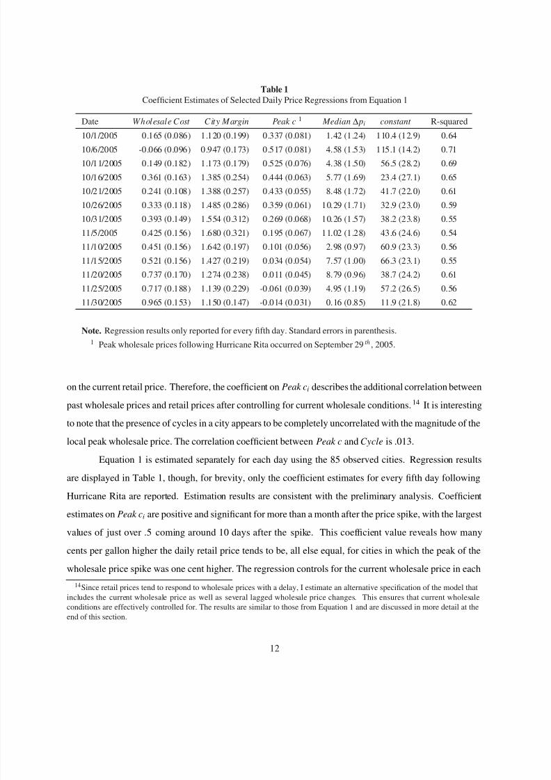
Figure 5. Predicted differences in retail margins between cities with high and low wholesale price spikes afterHurricane Rita. Wholesale prices peaked on September 29, 2005 in all cities.

-$0.05

$0.00

$0.05

$0.10

$0.15

3 0 - S e p

- 0 5

7 - O c t -

0 5

1 4 - O c t - 0 5

2 1 - O c t - 0 5

2 8 - O c t - 0 5

4 - N o

v - 0 5

1 1 - N o v - 0 5

1 8 - N o v - 0 5


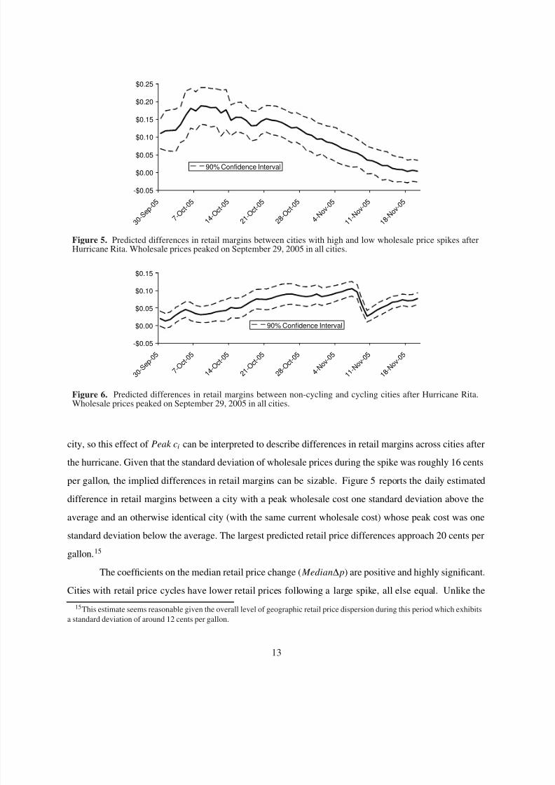
Figure 6. Predicted differences in retail margins between non-cycling and cycling cities after Hurricane Rita.Wholesale prices peaked on September 29, 2005 in all cities.

city, so this effect of Peak ci can be interpreted to describe differences in retail margins across cities after

the hurricane. Given that the standard deviation of wholesale prices during the spike was roughly 16 cents

per gallon, the implied differences in retail margins can be sizable. Figure 5 reports the daily estimated

difference in retail margins between a city with a peak wholesale cost one standard deviation above the

average and an otherwise identical city (with the same current wholesale cost) whose peak cost was one

standard deviation below the average. The largest predicted retail price differences approach 20 cents per

gallon.15

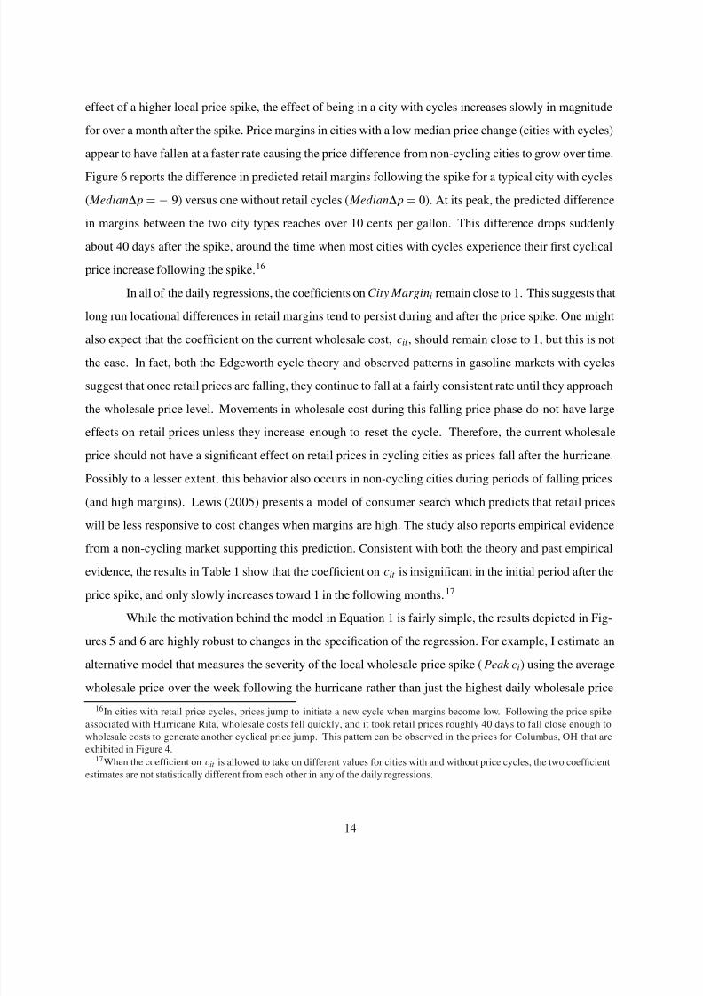
The coefficients on the median retail price change ( Median∆ p) are positive and highly significant.

Cities with retail price cycles have lower retail prices following a large spike, all else equal. Unlike the

15This estimate seems reasonable given the overall level of geographic retail price dispersion during this period which exhibits

a standard deviation of around 12 cents per gallon.

13



effect of a higher local price spike, the effect of being in a city with cycles increases slowly in magnitude

for over a month after the spike. Price margins in cities with a low median price change (cities with cycles)

appear to have fallen at a faster rate causing the price difference from non-cycling cities to grow over time.

Figure 6 reports the difference in predicted retail margins following the spike for a typical city with cycles

( Median∆ p = −.9) versus one without retail cycles ( Median∆ p = 0). At its peak, the predicted difference

in margins between the two city types reaches over 10 cents per gallon. This difference drops suddenly

about 40 days after the spike, around the time when most cities with cycles experience their first cyclical

price increase following the spike.16

In all of the daily regressions, the coefficients on City Margini remain close to 1. This suggests that

long run locational differences in retail margins tend to persist during and after the price spike. One might

also expect that the coefficient on the current wholesale cost, cit , should remain close to 1, but this is not

the case. In fact, both the Edgeworth cycle theory and observed patterns in gasoline markets with cycles

suggest that once retail prices are falling, they continue to fall at a fairly consistent rate until they approach

the wholesale price level. Movements in wholesale cost during this falling price phase do not have large

effects on retail prices unless they increase enough to reset the cycle. Therefore, the current wholesale

price should not have a significant effect on retail prices in cycling cities as prices fall after the hurricane.

Possibly to a lesser extent, this behavior also occurs in non-cycling cities during periods of falling prices

(and high margins). Lewis (2005) presents a model of consumer search which predicts that retail prices

will be less responsive to cost changes when margins are high. The study also reports empirical evidence

from a non-cycling market supporting this prediction. Consistent with both the theory and past empirical

evidence, the results in Table 1 show that the coefficient on cit is insignificant in the initial period after the

price spike, and only slowly increases toward 1 in the following months.17

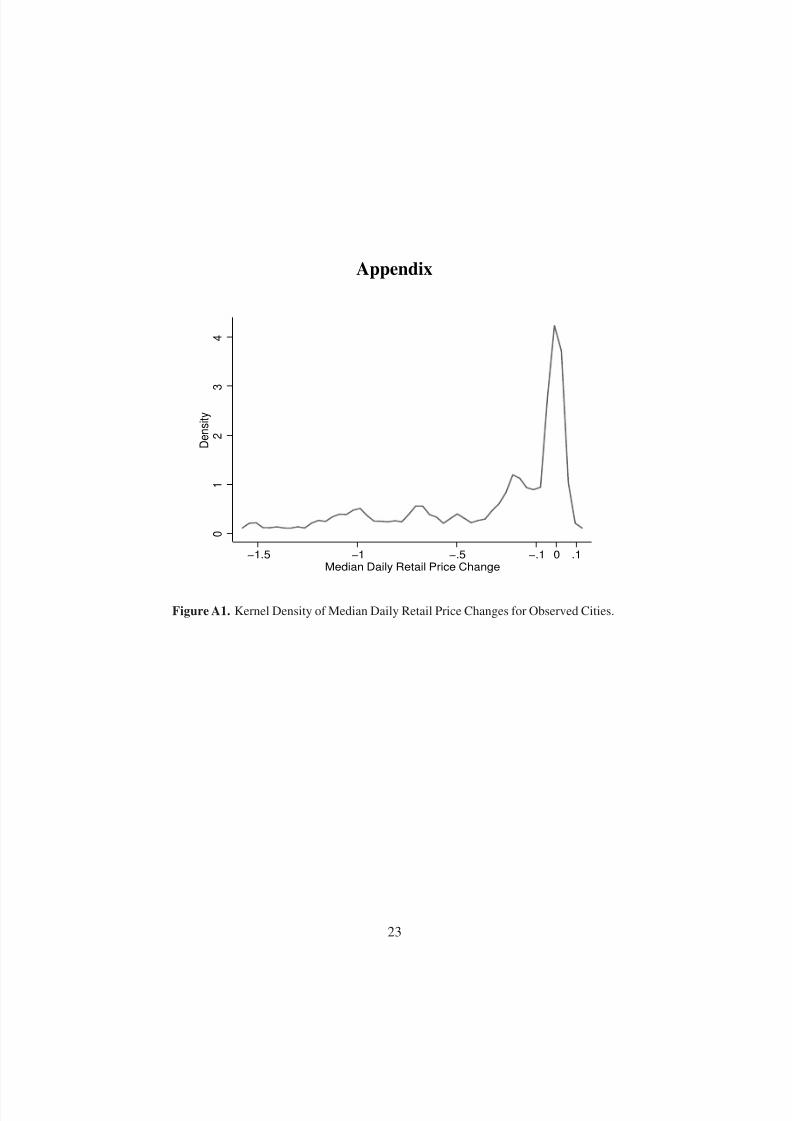
While the motivation behind the model in Equation 1 is fairly simple, the results depicted in Fig-

ures 5 and 6 are highly robust to changes in the specification of the regression. For example, I estimate an

alternative model that measures the severity of the local wholesale price spike ( Peak ci) using the average

wholesale price over the week following the hurricane rather than just the highest daily wholesale price

16In cities with retail price cycles, prices jump to initiate a new cycle when margins become low. Following the price spike

associated with Hurricane Rita, wholesale costs fell quickly, and it took retail prices roughly 40 days to fall close enough to

wholesale costs to generate another cyclical price jump. This pattern can be observed in the prices for Columbus, OH that are

exhibited in Figure 4.17When the coefficient on cit is allowed to take on different values for cities with and without price cycles, the two coefficient

estimates are not statistically different from each other in any of the daily regressions.

14



observed. The results of this estimation are very similar to those presented above. The estimated impacts

of cycles and peak wholesale prices on the observed retail prices using these alternative specifications are

presented in Appendix Figures A2 and A3 in a format comparable to that in Figures 5 and 6. In addition,

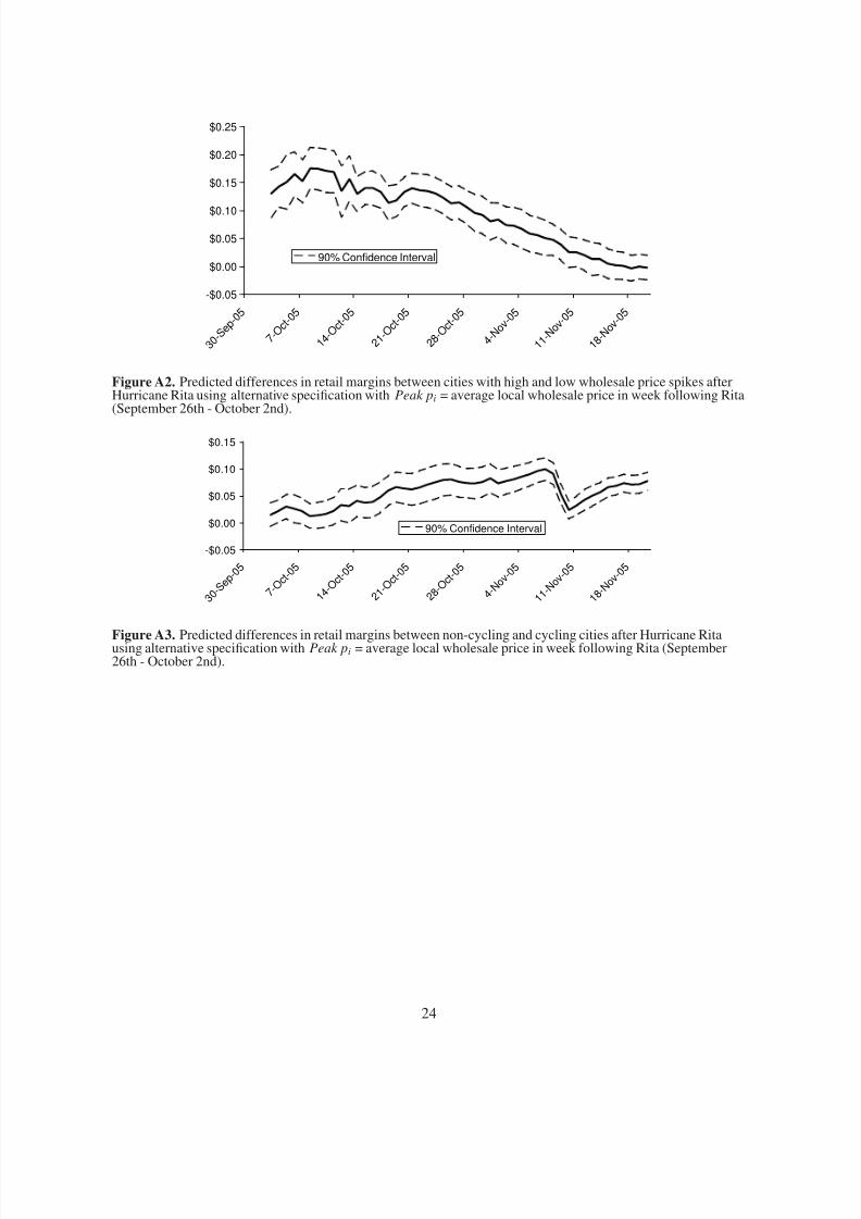
given that retailers may not experience a change in cost from their suppliers instantaneously after local

distribution rack prices change, I also consider controlling for the impact of lagged cost changes as well as

the current wholesale cost. I account for these by adding daily changes in wholesale cost over the previous

5 days as explanatory variables in Equation 1. Similar patterns are observed using this specification as

well. However, the estimates are a bit noisier, and the predicted impact of a higher peak wholesale price is

slightly smaller. The results from this specification are presented in Appendix Figures A4 and A5.

4.3. Impact on Consumers

Consumers paid higher retail prices following the hurricanes, not only because higher wholesale

costs were passed through, but also because retail margins increased. This appears to have been more

extreme in cities with larger wholesale price spikes. The estimation results imply that, over the six weeks

following Hurricane Rita, a city in which the wholesale price spiked 16 cents higher (2 standard deviations)

would have paid retail margins of 12.6 cents more on average than in an otherwise identical city. In addition

to higher wholesale costs being passed through, the higher retail margins alone would have caused a 15

gallon-per-week consumer to pay $11.33 (or over 6%) more for gasoline in this city over this period.

Following the price spike, consumers in cities without retail price cycles also paid higher retail margins

than consumers in otherwise identical cities with retail cycles. Over the eight weeks following Hurricane

Rita, consumers paid an average of 6.4 cents more in cities without retail price cycles, costing a 15 gallon-

per-week consumer an additional $7.64 over this period.

5. Where Do Retail Price Cycles Occur?

The empirical evidence suggests that retail prices and margins tend to differ significantly between

cities with and without retail price cycles following large wholesale market shocks. The importance of thepresence of cycles highlights the largely unanswered question of why cycles exist in some markets and not

others. The relatively large sample of cites in my data set is well suited for some further investigation into

this question.

The theory of Maskin and Tirole (1988) identifies a cyclical price equilibrium, but does not address

15



when this equilibrium might occur instead of a more stable equilibrium. Eckert (2003) introduces the idea

of heterogeneous firm size by assuming that when the two firms in the Maskin and Tirole model charge the

same price they receive an asymmetric split of the market. He shows that if one firm is assumed to receive

a sufficiently small share of the market when prices are equal, their incentive to undercut is strong enough

so that only the cyclical equilibrium exists. Noel (2007) compares retail gasoline pricing behavior in 19

Canadian cities (during the 1990’s) to test the predictions of Eckert (2003). Noel confirms that cities with

greater penetration of small independent sellers are more likely to exhibit price cycles.

The predictions from Eckert’s stylized model of equilibrium with different sized firms are roughly

borne out in the data. Aside from this, however, there is little theoretical guidance on how other more

complex factors in the retail gasoline market will affect price cycling behavior. For example, the ability to

coordinate price movements could be influenced by the presence of firms that own many stations and make

joint pricing decisions among multiple stations.18 Alternatively, heterogeneous tastes for gasoline from

different sellers (such as branded vs unbranded) could affect stations’ residual demand elasticities and cause

some to have greater incentives to match or undercut their competitors. Differences in consumer search

costs could have similar effects on the perceived residual demand elasticity. Noel (2007) suggests that a

higher density of potential consumers might increase the payoff from undercutting. He also suggests that

consumers might be better informed about prices (or have lower search costs) when the density of stations

is greater, which would also increase the potential payoff from undercutting. Confirming his intuition, Noel

(2007) finds empirical evidence that cities with greater population density per outlet and greater station

density are more likely to exhibit retail price cycles and that those cycles are likely to be more pronounced.

Using my measure of price cycling and my large cross-section of cities, I am able to estimate some

auxiliary regressions that help indicate which market characteristics are associated with the prominence of

cycles. I collect information on the share of independent stations, the density of stations, and the population

per station similar to the measures used in Noel (2007), plus a number of additional market characteristics.

Demographic information including population, land area, median income, median home value, average

number of cars per household, and average commute times are gathered from the 2000 U.S. Decennial

Census for the metropolitan statistical areas (MSAs) that appear in my price sample. I also obtain total

retail gasoline station counts for each MSA from the 2002 U.S. Economic Census. While the Economic

18It is important to note that pricing decisions at stations that are owned by the same company may not be jointly determined.

Stations owned by integrated refining companies are often leased to a dealer who operates the station and chooses the price at

which it resells the company’s branded gasoline.

16



Census does not provide information on the type or brand of stations, station counts of each brand are

available for the stations from which OPIS collects retail price information.19 While the OPIS sample

does not include all stations in a given MSA, it typically includes roughly 80% of stations in the area.

The OPIS data is used to calculate each brand’s market share within each city. These include integrated

refining company brands (such as BP and Shell), independent gasoline marketing chain brands (such as

Speedway and QuikTrip), and other retailers with a large gasoline marketing presence (such as Wal-Mart

and Kroger).20

In order to identify the market characteristics that are significantly associated with price cycles I

estimate a number of cross-sectional regressions of a city’s median price change on various market charac-

teristics. I analyze 83 cities for which I have both retail pricing data and comparable demographic infor-

mation.21 The base specification includes regressors found by Noel (2007) to be significantly associated

with the presence of retail cycles: the share of independent stations in the city, the average population per

station, and the average number of stations per square mile. In addition, I add several other demographic

variables that could be potentially related to consumers’ search or travel costs, or consumers’ willingness to

switch between brands or stations. These additional variables are median household income, median home

value, mean number of vehicles per household, and mean commuting time.

I present the results of the baseline specification in Table 2, Column 1. The median price change is

significantly lower (meaning cycles are more likely to occur) in cities with a higher population per station

or a higher share of independent stations. The baseline specification suggests that a city with a population

per station of one standard deviation above the mean has a median price change of .31 cents per gallon

lower than a city with a population per station of one standard deviation below the mean. In other words,

cities with greater population per station are more likely to have price cycles, or the price cycles in such

cities are likely to be more pronounced. Similarly, cities in which the market share of independent stations

19Station counts for each brand are collected from the OPIS Rack-To-Retail Margin Report from October 6, 2005. This report

is based on the same retail price data from which my daily city average prices are calculated.20Speedway is actually a wholly owned subsidiary of Marathon Petroleum. Despite this, the Speedway division operates its

retail stations independently of Marathon’s stations. They are not required to sell Marathon gasoline, and they behave very much

like an independent chain, so I consider them as such.21For this analysis I use 3 cities not used in the earlier price regressions because of a lack of wholesale price information

(Birmingham, AL, Moline-Rock Island, IL, and Peoria, IL), and I do not use 4 cities that were used in the price regressions

because they are not contained in proper MSAs, and therefore do not have comparable demographic information to the remaining

cities (Muskegon, MI, Traverse City, MI, Quincy, IL, and South Bend, IN). Chicago is also excluded from these regressions

because its population per station represents an extreme outlier. The highest population per station of any city (excluding Chicago)

is roughly 3 standard deviations above the mean population per city in the sample. Chicago’s value would be over 12 standard

deviations above the mean.

17



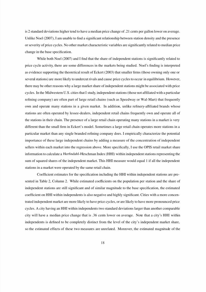
is 2 standard deviations higher tend to have a median price change of .21 cents per gallon lower on average.

Unlike Noel (2007), I am unable to find a significant relationship between station density and the presence

or severity of price cycles. No other market characteristic variables are significantly related to median price

change in the base specification.

While both Noel (2007) and I find that the share of independent stations is significantly related to

price cycle activity, there are some differences in the markets being studied. Noel’s finding is interpreted

as evidence supporting the theoretical result of Eckert (2003) that smaller firms (those owning only one or

several stations) are more likely to undercut rivals and cause price cycles to occur in equilibrium. However,

there may be other reasons why a large market share of independent stations might be associated with price

cycles. In the Midwestern U.S. cities that I study, independent stations (those not affiliated with a particular

refining company) are often part of large retail chains (such as Speedway or Wal-Mart) that frequently

own and operate many stations in a given market. In addition, unlike refinery-affiliated brands whose

stations are often operated by lessee-dealers, independent retail chains frequently own and operate all of

the stations in their chain. The presence of a large retail chain operating many stations in a market is very

different than the small firm in Eckert’s model. Sometimes a large retail chain operates more stations in a

particular market than any single branded refining company does. I empirically characterize the potential

importance of these large independent chains by adding a measure of the concentration of independent

sellers within each market into the regression above. More specifically, I use the OPIS retail market share

information to calculate a Herfindahl-Hirschman Index (HHI) within independent stations representing the

sum of squared shares of the independent market. This HHI measure would equal 1 if all the independent

stations in a market were operated by the same retail chain.

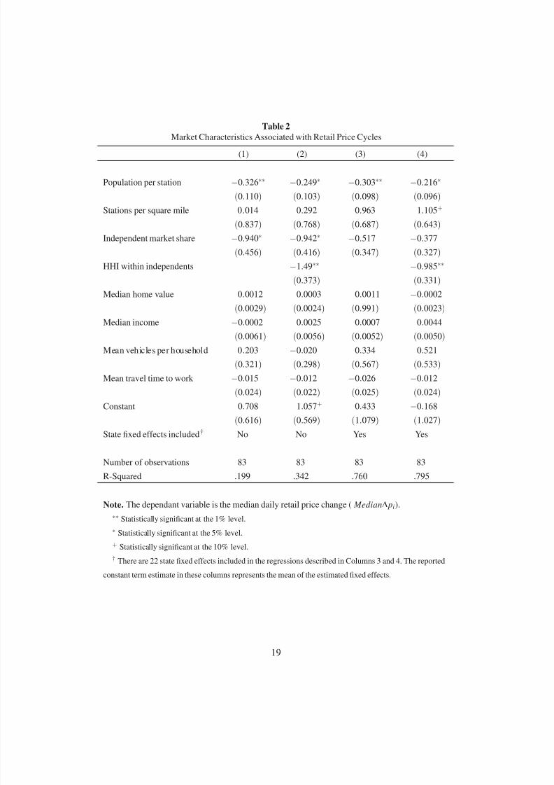
Coefficient estimates for the specification including the HHI within independent stations are pre-

sented in Table 2, Column 2. While estimated coefficients on the population per station and the share of

independent stations are still significant and of similar magnitude to the base specification, the estimated

coefficient on HHI within independents is also negative and highly significant. Cities with a more concen-

trated independent market are more likely to have price cycles, or are likely to have more pronounced price

cycles. A city having an HHI within independents two standard deviations larger than another comparable

city will have a median price change that is .36 cents lower on average. Note that a city’s HHI within

independents is defined to be completely distinct from the level of the city’s independent market share,

so the estimated effects of these two measures are unrelated. Moreover, the estimated magnitude of the

18



Table 2

Market Characteristics Associated with Retail Price Cycles

(1) (2) (3) (4)

Population per station −0.326∗∗ −0.249∗ −0.303∗∗ −0.216∗

(0.110) (0.103) (0.098) (0.096)

Stations per square mile 0.014 0.292 0.963 1.105+

(0.837) (0.768) (0.687) (0.643)

Independent market share −0.940∗ −0.942∗ −0.517 −0.377

(0.456) (0.416) (0.347) (0.327)

HHI within independents −1.49∗∗ −0.985∗∗

(0.373) (0.331)

Median home value 0.0012 0.0003 0.0011 −0.0002

(0.0029) (0.0024) (0.991) (0.0023)

Median income −0.0002 0.0025 0.0007 0.0044

(0.0061) (0.0056) (0.0052) (0.0050)

Mean vehicles per household 0.203 −0.020 0.334 0.521

(0.321) (0.298) (0.567) (0.533)

Mean travel time to work −0.015 −0.012 −0.026 −0.012

(0.024) (0.022) (0.025) (0.024)

Constant 0.708 1.057+ 0.433 −0.168

(0.616) (0.569) (1.079) (1.027)

State fixed effects included† No No Yes Yes

Number of observations 83 83 83 83

R-Squared .199 .342 .760 .795

Note. The dependant variable is the median daily retail price change ( Median∆ pi).

∗∗ Statistically significant at the 1% level.

∗ Statistically significant at the 5% level.

+

Statistically significant at the 10% level.† There are 22 state fixed effects included in the regressions described in Columns 3 and 4. The reported

constant term estimate in these columns represents the mean of the estimated fixed effects.

19



effect of having a higher HHI within independents suggests that the concentration of a city’s independent

stations is a stronger indicator of price cycle activity than the overall share of independents in the market.

The relationship between price cycles and the concentration of independent stations has not been previously

studied, and suggests that independent stations may play an important role in the market that is not captured

in the Eckert (2003) model of Edgeworth cycles and firm size.

The results above give some indication of the types of cities that are more likely to exhibit cyclical

retail pricing. However, much of the geographic variation in the extent of cyclical pricing behavior is not

captured by the observed variables. Casual observation suggests that the presence of price cycles may

be geographically correlated, as cycles tend to appear in one part of the Midwestern U.S. but not in the

rest of the country. Many unobservable geographic market factors could produce this correlation, such as,

regional differences in consumers’ demand or level of price information, or regional differences in the types

or identities of firms competing in the retail market. Regardless of the source, it may be informative to study

whether the differences in market characteristics that have been generally identified between cycling and

non-cycling regions are also present between cycling and non-cycling cities within the same geographic

region. I therefore re-estimate the two specifications above while including state fixed effects to identify

differences in market characteristics within a particular state that are associated with differences in the

presence or intensity of price cycles occurring in cities within the state.

The results of the state fixed effects regressions are reported in Table 2, Columns 3 and 4, and are

analogous to the specifications in Columns 1 and 2 respectively. As expected, the state fixed effects capture

a large share of the geographic variation in cyclical pricing behavior. The coefficient estimates of how

market characteristics relate to the remaining within-state variation in cyclical pricing are largely consistent

with those estimated overall in Columns 1 and 2. The most notable difference is that independent market

share is not a significant predictor of cyclical pricing activity, whereas the HHI within independent stations

remains a highly significant predictor of differences in price cycles within a state. 22

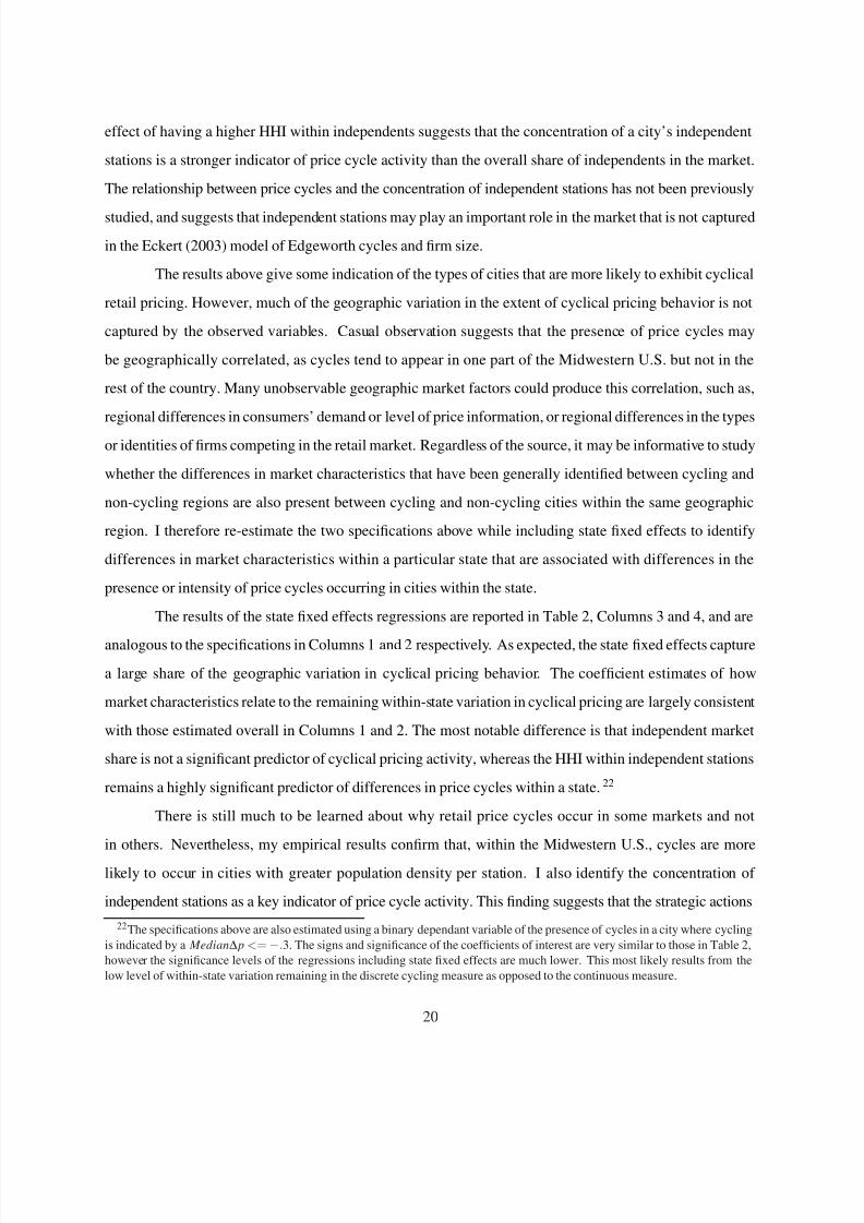
There is still much to be learned about why retail price cycles occur in some markets and not

in others. Nevertheless, my empirical results confirm that, within the Midwestern U.S., cycles are more

likely to occur in cities with greater population density per station. I also identify the concentration of

independent stations as a key indicator of price cycle activity. This finding suggests that the strategic actions

22The specifications above are also estimated using a binary dependant variable of the presence of cycles in a city where cycling

is indicated by a Median∆ p <=−.3. The signs and significance of the coefficients of interest are very similar to those in Table 2,

however the significance levels of the regressions including state fixed effects are much lower. This most likely results from the

low level of within-state variation remaining in the discrete cycling measure as opposed to the continuous measure.

20



of large independent retail chains may contribute to the formation of cyclical price equilibria, and that

further research into the roles of multi-station firms and the conditions of cyclical equilibria are necessary.

6. Conclusions

Retail prices remained significantly higher after Hurricane Rita in cities experiencing a larger ini-

tial wholesale price spike and in cities that are not known to exhibit retail price cycles. Due to the descrip-

tive nature of the empirical analysis, the source of these relationships is not empirically identified here.

Nonetheless, these patterns are valuable in understanding what factors may be related to existence of large

temporary geographic differences in retail prices (and margins). This is particularly true given the relative

lack of understanding of the market attributes that generate Edgeworth price cycles and of the impact of

Edgeworth cycles on competition and market power. Interpreting these empirical results in the context of the existing economic theory and the institutions of gasoline markets yields several additional conclusions.

The asymmetric retail gasoline price response literature extensively documents patterns of higher

margins and delayed response to wholesale price declines. The first set of empirical results from this

study expand on this literature by highlighting how asymmetric retail price response can cause a temporary

wholesale price spike to have long-lasting impacts on retail prices. If the severity of the temporary whole-

sale price spikes varies geographically, this can generate persistent geographic dispersion in retail prices.

In addition, large differences between cities in the speed with which retail prices fall after a temporary

price spike can also generate significant geographic dispersion in retail prices even if the magnitude of the

wholesale spike was relatively uniform across cities.

Persistent retail price effects from temporary price spikes suggest interesting implications regarding

the ability and/or incentive for large refining companies to exercise market power during periods when

refining capacity is tight. Generally, the incentives for refiners to exercise market power in the wholesale

gasoline market increase when capacity is scarce and prices are already high (see Borenstein, Bushnell, and

Lewis (2004)). Many of these large refiners also capture retail margins by selling through their own stations

or by selling to their branded dealer stations at prices well above the unbranded wholesale price observedin this study. Integrated refiners may have even more incentive to temporarily exercise wholesale market

power during price spikes if it also increases profits from future retail margins.

The second set of empirical results from this study focus on the importance of retail price cycles.

I show that cities with retail price cycles had lower prices (and margins) than otherwise comparable cities

21



during the weeks after Hurricane Rita. This finding does not itself imply that the existence of cycles caused

prices to be lower.23 However, the dynamic properties of the Edgeworth cycle equilibrium provide an

explanation for why cycles could be responsible for more rapid declines in price. In most (non-cycling)

cities, retail gasoline prices are fairly sticky and respond slowly to cost changes. In contrast, when cycling

cities are in the undercutting phase of the cycle, firms’ default everyday behavior is to reduce price. In

a practical sense, no adjustment in behavior is needed for retail prices to continue falling after wholesale

costs have dropped. This unique feature of the cyclical equilibrium price dynamic serves as a possible

explanation for the more rapid price declines observed in cycling cities after Hurricane Rita and the large

differences in retail prices between cycling and non-cycling cities during this period.

Finally, the small and growing literature on retail price cycles in gasoline markets has yet to deter-

mine whether markets with cycles tend to be more or less competitive, and to what extent competitiveness

generates or is a product of retail price cycles. The empirical findings presented here give some additional

clues in this puzzle by showing that cities with cycles do have lower prices (and margins) than other cities

during periods following a significant wholesale price spikes. In addition, the cross-sectional analysis re-

veals differences in market characteristics between cycling and non-cycling cities, and identifies that large

independent retail chains may play an important role in the existence of retail cycles.

23It is possible that cycles occur for some reason in cities where retail prices also tend to fall quickly after wholesale prices fall.

22



Appendix

0

1

2

3

4

D e n s i t y

−1.5 −1 −.5 −.1 0 .1Median Daily Retail Price Change

Figure A1. Kernel Density of Median Daily Retail Price Changes for Observed Cities.

23



-$0.05

$0.00

$0.05

$0.10

$0.15

$0.20

$0.25

3 0 - S e p

- 0 5

7 - O c t

- 0 5

1 4 - O c t

- 0 5

2 1 - O c t

- 0 5

2 8 - O c t

- 0 5

4 - N o

v - 0 5

1 1 - N o v - 0 5

1 8 - N o v - 0 5


Figure A2. Predicted differences in retail margins between cities with high and low wholesale price spikes afterHurricane Rita using alternative specification with Peak pi = average local wholesale price in week following Rita(September 26th - October 2nd).

-$0.05

$0.00

$0.05

$0.10

$0.15

3 0 - S e p

- 0 5

7 - O c t - 0 5

1 4 - O c t -

0 5

2 1 - O c t -

0 5

2 8 - O c t -

0 5

4 - N o

v - 0 5

1 1 - N o v - 0 5

1 8 - N o v - 0 5


Figure A3. Predicted differences in retail margins between non-cycling and cycling cities after Hurricane Ritausing alternative specification with Peak pi = average local wholesale price in week following Rita (September26th - October 2nd).

24



-$0.05

$0.00

$0.05

$0.10

$0.15

$0.20

$0.25

3 0 - S e p

- 0 5

7 - O c t

- 0 5

1 4 - O c t -

0 5

2 1 - O c t -

0 5

2 8 - O c t -

0 5

4 - N o

v - 0 5

1 1 - N o v - 0 5

1 8 - N o v - 0 5


Figure A4. Predicted differences in retail margins between cities with high and low wholesale price spikes afterHurricane Rita using alternate specification with 5 days of lagged wholesale cost changes included in controls.

-$0.05

$0.00

$0.05

$0.10

$0.15

3 0 - S e p

- 0 5

7 - O c t - 0 5

1 4 - O c t - 0 5

2 1 - O c t - 0 5

2 8 - O c t - 0 5

4 - N o

v - 0 5

1 1 - N o v - 0 5

1 8 - N o v - 0 5


Figure A5. Predicted differences in retail margins between non-cycling and cycling cities after Hurricane Rita

using alternate specification with 5 days of lagged wholesale cost changes included in controls.

25



References

Borenstein, Severin, James Bushnell, and Matthew Lewis. 2004. “Market Power in California’s Gasoline

Market.” Center for the Study of Energy Markets Working Paper #132, The University of California

Energy Institute.

Borenstein, Severin, Colin Cameron, and Richard Gilbert. 1997. “Do Gasoline Prices Respond Asymmet-

rically to Crude Oil Price Changes?” The Quarterly Journal of Economics 112:306–339.

Castanias, Rick and Herb Johnson. 1993. “Gas Wars: Retail Gasoline Price Fluctuations.” Review of

Economics and Statistics 75:171–174.

Deltas, George. Forthcoming. “Retail Gasoline Price Dynamics and Local Market Power.” Journal of

Industrial Economics .

Eckert, Andrew. 2003. “Retail Price Cycles and the Presence of Small Firms.” International Journal of

Industrial Organization 21:151–170.

Eckert, Andrew and Douglas West. 2004. “A Tale of Two Cities: Price Uniformity and Price Volatility in

Gasoline Retailing.” The Annals of Regional Science 38:25–46.

Hibbard, Paul J. 2006. “US Energy Infrastructure Vulnerability: Lessons From the Gulf Coast Hurricanes.”

Analysis Group Report.

Lewis, Matthew. 2005. “Asymmetric Price Adjustment and Consumer Search: An Examination of the

Retail Gasoline Market.” Working paper. The Ohio State University, Columbus, OH.

Maskin, Eric and Jean Tirole. 1988. “A Theory of Dynamic Oligopoly II: Price Competition, Kinked

Demand Curves, and Edgeworth Cycles.” Econometrica 56:571–599.

Noel, Michael. 2007. “Edgeworth Price Cycles: Cost Based Pricing and Sticky Pricing in Retail Gasoline

Markets.” Review of Economics and Statistics 89:324–334.

U.S. Federal Trade Commission. 2006. “Investigation of Gasoline Price Manipulation and Post-Katrina

Gasoline Price Increases.” Washington, D.C.

Verlinda, Jeremy A. Forthcoming. “Do Rockets Rise Faster and Feathers Fall Slower in an Atmosphere of

Local Market Power? Evidence from the Retail Gasoline Market.” Journal of Industrial Economics .

26



Wang, Zhongmin. 2006. “Cartel Communication and Price Coordination: A Case Study.” Working Paper.

Northeastern University, Boston, MA.

27

Documents

Gas Price Spikes.1