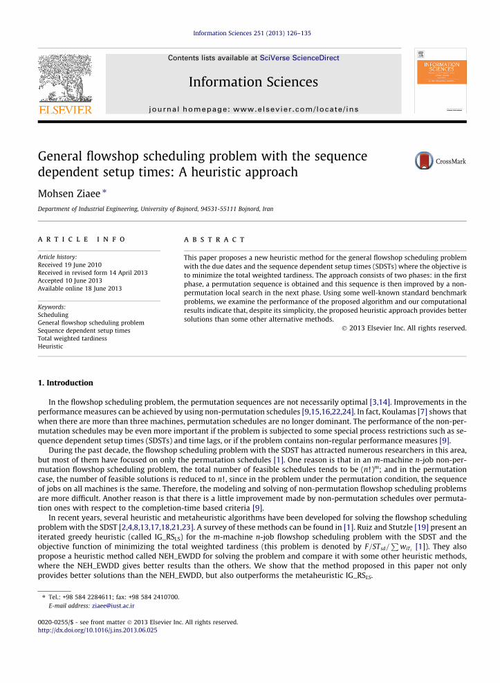
Information Sciences 251 (2013) 126–135

Contents lists available at SciVerse ScienceDirect

Information Sciences

journal homepage: www.elsevier .com/locate / ins

General flowshop scheduling problem with the sequencedependent setup times: A heuristic approach

0020-0255/$ - see front matter � 2013 Elsevier Inc. All rights reserved.http://dx.doi.org/10.1016/j.ins.2013.06.025

⇑ Tel.: +98 584 2284611; fax: +98 584 2410700.E-mail address: ziaee@iust.ac.ir

Mohsen Ziaee ⇑Department of Industrial Engineering, University of Bojnord, 94531-55111 Bojnord, Iran

a r t i c l e i n f o

Article history:Received 19 June 2010Received in revised form 14 April 2013Accepted 10 June 2013Available online 18 June 2013

Keywords:SchedulingGeneral flowshop scheduling problemSequence dependent setup timesTotal weighted tardinessHeuristic

a b s t r a c t

This paper proposes a new heuristic method for the general flowshop scheduling problemwith the due dates and the sequence dependent setup times (SDSTs) where the objective isto minimize the total weighted tardiness. The approach consists of two phases: in the firstphase, a permutation sequence is obtained and this sequence is then improved by a non-permutation local search in the next phase. Using some well-known standard benchmarkproblems, we examine the performance of the proposed algorithm and our computationalresults indicate that, despite its simplicity, the proposed heuristic approach provides bettersolutions than some other alternative methods.

� 2013 Elsevier Inc. All rights reserved.

1. Introduction

In the flowshop scheduling problem, the permutation sequences are not necessarily optimal [3,14]. Improvements in theperformance measures can be achieved by using non-permutation schedules [9,15,16,22,24]. In fact, Koulamas [7] shows thatwhen there are more than three machines, permutation schedules are no longer dominant. The performance of the non-per-mutation schedules may be even more important if the problem is subjected to some special process restrictions such as se-quence dependent setup times (SDSTs) and time lags, or if the problem contains non-regular performance measures [9].

During the past decade, the flowshop scheduling problem with the SDST has attracted numerous researchers in this area,but most of them have focused on only the permutation schedules [1]. One reason is that in an m-machine n-job non-per-mutation flowshop scheduling problem, the total number of feasible schedules tends to be (n!)m; and in the permutationcase, the number of feasible solutions is reduced to n!, since in the problem under the permutation condition, the sequenceof jobs on all machines is the same. Therefore, the modeling and solving of non-permutation flowshop scheduling problemsare more difficult. Another reason is that there is a little improvement made by non-permutation schedules over permuta-tion ones with respect to the completion-time based criteria [9].

In recent years, several heuristic and metaheuristic algorithms have been developed for solving the flowshop schedulingproblem with the SDST [2,4,8,13,17,18,21,23]. A survey of these methods can be found in [1]. Ruiz and Stutzle [19] present aniterated greedy heuristic (called IG_RSLS) for the m-machine n-job flowshop scheduling problem with the SDST and theobjective function of minimizing the total weighted tardiness (this problem is denoted by F=STsd=

PwiTi

[1]). They alsopropose a heuristic method called NEH_EWDD for solving the problem and compare it with some other heuristic methods,where the NEH_EWDD gives better results than the others. We show that the method proposed in this paper not onlyprovides better solutions than the NEH_EWDD, but also outperforms the metaheuristic IG_RSLS.

M. Ziaee / Information Sciences 251 (2013) 126–135 127

In this paper, the problem F=STsd=P

wiTiis considered and a two-phase heuristic method is presented to solve the prob-

lem (Section 2), where the main purpose is to produce suboptimal schedules, very quickly. It can further be used for improv-ing the quality of the initial feasible solution of metaheuristics applied to solve the problem. It should be noted that thechoice of a good-initial solution plays an important role in the performance of algorithms in terms of solution quality andcomputational time [3,5,10,14]. In the heuristic algorithm proposed in this paper, the effect of changing the permutationschedules into the non-permutation ones over the improvement of the objective function value is studied. In the first phaseof the algorithm, a permutation sequence is obtained. This sequence is then improved by a non-permutation local search inthe next phase. Therefore, the final solution produced by the method may be a non-permutation schedule. Then, in order toevaluate the performance of the heuristic approach, the author performs computational experiments by using well-knownbenchmark problems provided by Taillard [20] and augmented by Ruiz and Stutzle [19] to include the SDST (Section 3).

The notations used in the paper are as follows:

n

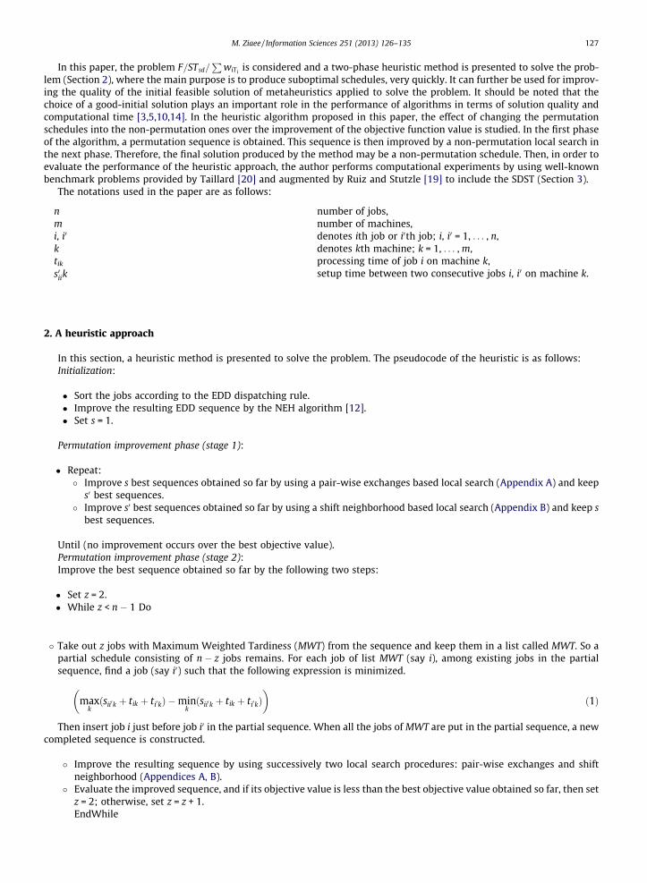
number of jobs, m number of machines, i, i0 denotes ith job or i0th job; i, i0 = 1, . . . , n, k denotes kth machine; k = 1, . . . , m, tik processing time of job i on machine k, s0iik setup time between two consecutive jobs i, i0 on machine k.

2. A heuristic approach

In this section, a heuristic method is presented to solve the problem. The pseudocode of the heuristic is as follows:Initialization:

� Sort the jobs according to the EDD dispatching rule.� Improve the resulting EDD sequence by the NEH algorithm [12].� Set s = 1.

Permutation improvement phase (stage 1):

� Repeat:� Improve s best sequences obtained so far by using a pair-wise exchanges based local search (Appendix A) and keep

s0 best sequences.� Improve s0 best sequences obtained so far by using a shift neighborhood based local search (Appendix B) and keep s

best sequences.

Until (no improvement occurs over the best objective value).Permutation improvement phase (stage 2):Improve the best sequence obtained so far by the following two steps:

� Set z = 2.� While z < n � 1 Do

� Take out z jobs with Maximum Weighted Tardiness (MWT) from the sequence and keep them in a list called MWT. So apartial schedule consisting of n � z jobs remains. For each job of list MWT (say i), among existing jobs in the partialsequence, find a job (say i0) such that the following expression is minimized.

maxkðsii0k þ tik þ ti0kÞ �min

kðsii0k þ tik þ ti0kÞ

� �ð1Þ

Then insert job i just before job i0 in the partial sequence. When all the jobs of MWT are put in the partial sequence, a newcompleted sequence is constructed.

� Improve the resulting sequence by using successively two local search procedures: pair-wise exchanges and shiftneighborhood (Appendices A, B).

� Evaluate the improved sequence, and if its objective value is less than the best objective value obtained so far, then setz = 2; otherwise, set z = z + 1.EndWhile

128 M. Ziaee / Information Sciences 251 (2013) 126–135

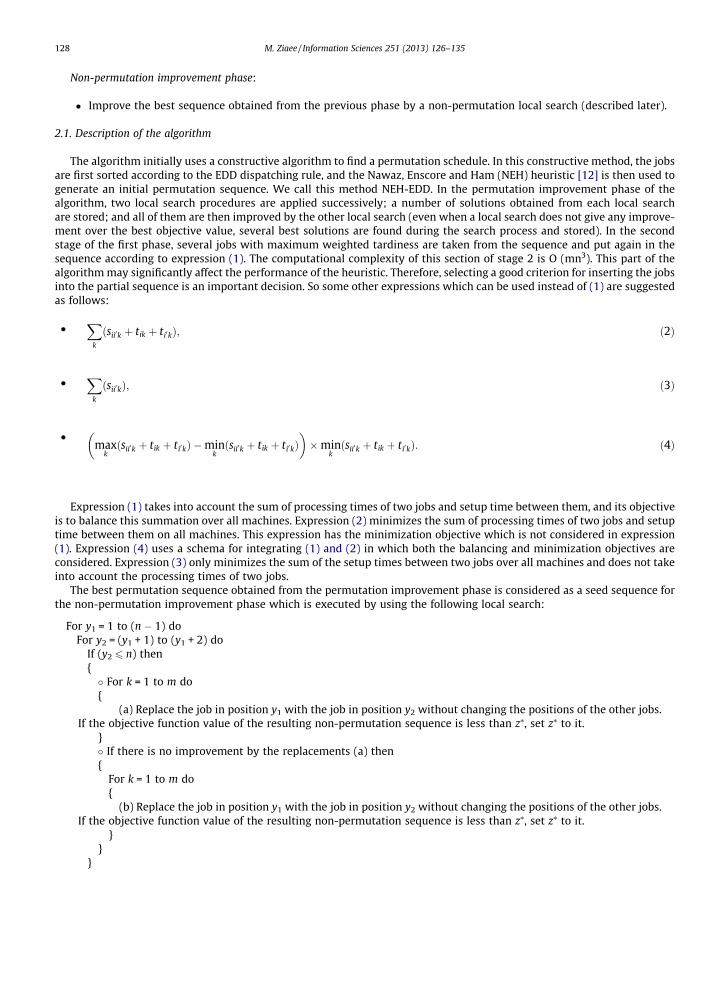
Non-permutation improvement phase:

� Improve the best sequence obtained from the previous phase by a non-permutation local search (described later).

2.1. Description of the algorithm

The algorithm initially uses a constructive algorithm to find a permutation schedule. In this constructive method, the jobsare first sorted according to the EDD dispatching rule, and the Nawaz, Enscore and Ham (NEH) heuristic [12] is then used togenerate an initial permutation sequence. We call this method NEH-EDD. In the permutation improvement phase of thealgorithm, two local search procedures are applied successively; a number of solutions obtained from each local searchare stored; and all of them are then improved by the other local search (even when a local search does not give any improve-ment over the best objective value, several best solutions are found during the search process and stored). In the secondstage of the first phase, several jobs with maximum weighted tardiness are taken from the sequence and put again in thesequence according to expression (1). The computational complexity of this section of stage 2 is O (mn3). This part of thealgorithm may significantly affect the performance of the heuristic. Therefore, selecting a good criterion for inserting the jobsinto the partial sequence is an important decision. So some other expressions which can be used instead of (1) are suggestedas follows:

� Xðsii0k þ tik þ ti0kÞ; ð2Þ

k

� Xðsii0kÞ; ð3Þ

k

� � �

max

kðsii0k þ tik þ ti0kÞ �min

kðsii0k þ tik þ ti0kÞ �min

kðsii0k þ tik þ ti0kÞ: ð4Þ

Expression (1) takes into account the sum of processing times of two jobs and setup time between them, and its objectiveis to balance this summation over all machines. Expression (2) minimizes the sum of processing times of two jobs and setuptime between them on all machines. This expression has the minimization objective which is not considered in expression(1). Expression (4) uses a schema for integrating (1) and (2) in which both the balancing and minimization objectives areconsidered. Expression (3) only minimizes the sum of the setup times between two jobs over all machines and does not takeinto account the processing times of two jobs.

The best permutation sequence obtained from the permutation improvement phase is considered as a seed sequence forthe non-permutation improvement phase which is executed by using the following local search:

For y1 = 1 to (n � 1) doFor y2 = (y1 + 1) to (y1 + 2) do

If (y2 6 n) then{� For k = 1 to m do{

(a) Replace the job in position y1 with the job in position y2 without changing the positions of the other jobs.If the objective function value of the resulting non-permutation sequence is less than z⁄, set z⁄ to it.

}� If there is no improvement by the replacements (a) then{

For k = 1 to m do{

(b) Replace the job in position y1 with the job in position y2 without changing the positions of the other jobs.If the objective function value of the resulting non-permutation sequence is less than z⁄, set z⁄ to it.

}}

}

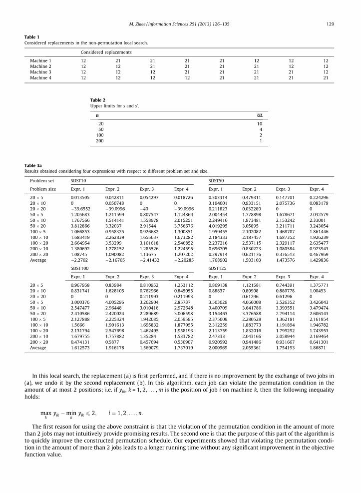
Table 1Considered replacements in the non-permutation local search.

Considered replacements

Machine 1 12 21 21 21 21 12 12 12Machine 2 12 12 21 21 21 21 12 12Machine 3 12 12 12 21 21 21 21 12Machine 4 12 12 12 12 21 21 21 21

Table 2Upper limits for s and s0 .

n UL

20 1050 4

100 2200 1

Table 3aResults obtained considering four expressions with respect to different problem set and size.

Problem set SDST10 SDST50

Problem size Expr. 1 Expr. 2 Expr. 3 Expr. 4 Expr. 1 Expr. 2 Expr. 3 Expr. 4

20 � 5 0.013505 0.042811 0.054297 0.018726 0.303314 0.479311 0.147701 0.22429620 � 10 0 0.050748 0 0 3.194001 0.933151 2.075736 0.08317920 � 20 �39.6552 �39.0996 �40 �39.0996 0.211823 0.032289 0 050 � 5 1.205683 1.211599 0.807547 1.124864 2.004454 1.778898 1.678671 2.03257950 � 10 1.767566 1.514141 1.558978 2.015251 2.249416 1.973481 2.153242 2.3300150 � 20 3.812866 3.32037 2.91544 3.756676 4.019295 3.05895 3.211711 3.243054100 � 5 1.066853 0.958325 0.926682 1.300851 1.959455 2.102082 1.468707 1.861446100 � 10 1.683419 2.262839 1.655637 1.673282 2.184333 2.187457 1.687352 1.926239100 � 20 2.664954 3.53299 3.101618 2.546852 2.237216 2.537115 2.329117 2.635477200 � 10 1.380692 1.278152 1.285526 1.224595 0.696705 0.830223 1.080584 0.923943200 � 20 1.08745 1.090082 1.13675 1.207202 0.397914 0.621176 0.376513 0.467969Average �2.2702 �2.16705 �2.41432 �2.20285 1.768902 1.503103 1.473576 1.429836

SDST100 SDST125

Expr. 1 Expr. 2 Expr. 3 Expr. 4 Expr. 1 Expr. 2 Expr. 3 Expr. 4

20 � 5 0.967958 0.83984 0.810952 1.253112 0.869138 1.121581 0.744391 1.37577120 � 10 0.831741 1.828105 0.762966 0.845055 0.88837 0.80908 0.880778 1.0049320 � 20 0 0 0.211993 0.211993 0 0.61296 0.61296 050 � 5 3.000376 4.005296 3.262904 2.85737 3.503029 4.066008 3.526352 3.42604350 � 10 2.547477 2.96448 3.010416 2.972648 3.400709 3.641786 3.393551 3.47947450 � 20 2.410586 2.420024 2.289689 3.006598 3.154463 3.376588 2.794114 2.606143100 � 5 2.127888 2.225324 1.942085 2.059595 2.375009 2.280528 1.362181 2.161954100 � 10 1.5666 1.901613 1.695832 1.877955 2.312259 1.883773 1.191894 1.946782100 � 20 2.131794 2.547698 1.462495 1.958193 2.113759 1.832016 1.799292 1.743953200 � 10 1.679755 1.757882 1.35284 1.533782 2.47333 2.043166 2.058944 2.169464200 � 20 0.474131 0.5877 0.457694 0.530907 0.920592 0.941486 0.931667 0.641301Average 1.612573 1.916178 1.569079 1.737019 2.000969 2.055361 1.754193 1.86871

M. Ziaee / Information Sciences 251 (2013) 126–135 129

In this local search, the replacement (a) is first performed, and if there is no improvement by the exchange of two jobs in(a), we undo it by the second replacement (b). In this algorithm, each job can violate the permutation condition in theamount of at most 2 positions; i.e. if yik, k = 1, 2, . . . , m is the position of job i on machine k, then the following inequalityholds:

maxk

yik �mink

yik 6 2; i ¼ 1;2; . . . ; n:

The first reason for using the above constraint is that the violation of the permutation condition in the amount of morethan 2 jobs may not intuitively provide promising results. The second one is that the purpose of this part of the algorithm isto quickly improve the constructed permutation schedule. Our experiments showed that violating the permutation condi-tion in the amount of more than 2 jobs leads to a longer running time without any significant improvement in the objectivefunction value.

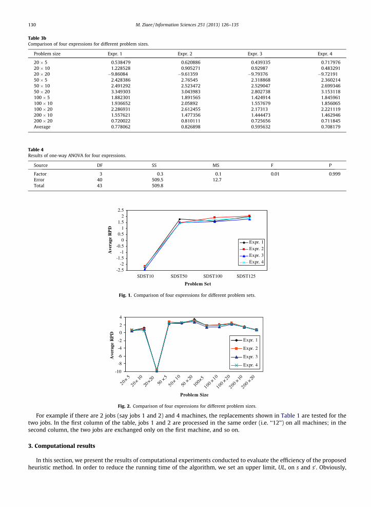
Table 3bComparison of four expressions for different problem sizes.

Problem size Expr. 1 Expr. 2 Expr. 3 Expr. 4

20 � 5 0.538479 0.620886 0.439335 0.71797620 � 10 1.228528 0.905271 0.92987 0.48329120 � 20 �9.86084 �9.61359 �9.79376 �9.7219150 � 5 2.428386 2.76545 2.318868 2.36021450 � 10 2.491292 2.523472 2.529047 2.69934650 � 20 3.349303 3.043983 2.802738 3.153118100 � 5 1.882301 1.891565 1.424914 1.845961100 � 10 1.936652 2.05892 1.557679 1.856065100 � 20 2.286931 2.612455 2.17313 2.221119200 � 10 1.557621 1.477356 1.444473 1.462946200 � 20 0.720022 0.810111 0.725656 0.711845Average 0.778062 0.826898 0.595632 0.708179

Table 4Results of one-way ANOVA for four expressions.

Source DF SS MS F P

Factor 3 0.3 0.1 0.01 0.999Error 40 509.5 12.7Total 43 509.8

-2.5-2

-1.5-1

-0.50

0.51

1.52

2.5

SDST10 SDST50 SDST100 SDST125

Problem Set

Ave

rage

RP

D

Expr. 1Expr. 2Expr. 3Expr. 4

Fig. 1. Comparison of four expressions for different problem sets.

-10

-8

-6

-4

-2

0

2

4

20×5

20×10

20×20

50×5

50×10

50×20

100×5

100 ×10

100 ×20

200 ×10

200 ×20

Problem Size

Ave

rage

RP

D

Expr. 1

Expr. 2

Expr. 3

Expr. 4

Fig. 2. Comparison of four expressions for different problem sizes.

130 M. Ziaee / Information Sciences 251 (2013) 126–135

For example if there are 2 jobs (say jobs 1 and 2) and 4 machines, the replacements shown in Table 1 are tested for thetwo jobs. In the first column of the table, jobs 1 and 2 are processed in the same order (i.e. ‘‘12’’) on all machines; in thesecond column, the two jobs are exchanged only on the first machine, and so on.

3. Computational results

In this section, we present the results of computational experiments conducted to evaluate the efficiency of the proposedheuristic method. In order to reduce the running time of the algorithm, we set an upper limit, UL, on s and s0. Obviously,

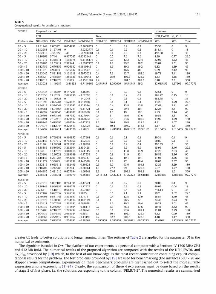
Table 5Computational results for benchmark instances.

SDST10 Proposed method Literature

RPD Time NEH_EWDD IG_RSLS

Problem size NEH-EDD PRMUT-1 PRMUT-2 NONPRMUT NEH-EDD PRMUT-1 PRMUT-2 NONPRMUT RPD RPD Time

20 � 5 28.91248 2.00327 0.054297 �2.2600277 0 0 0.2 0.2 25.53 0 920 � 10 52.42988 3.157408 0 �5.9252777 0.1 0.1 0.2 0.2 218.41 0 1820 � 20 9.552419 �38.8271 �40 �61.968981 0.1 0.1 0.3 0.3 492.98 0 3650 � 5 14.16962 3.744 0.807547 0.3292444 0 0.5 7.6 7.6 8.99 0.77 22.550 � 10 27.21213 8.338611 1.558978 �0.1126178 0 0.6 12.2 12.4 22.02 1.22 4550 � 20 80.39405 13.53217 2.91544 �5.9977775 0.1 1.1 29.2 30.2 93.04 1.51 90100 � 5 9.812759 2.676855 0.926682 0.4840846 0 1.6 19.2 19.2 6.82 1.39 45100 � 10 12.4137 4.92853 1.655637 0.678577 0.5 3 46.6 48 9.89 2.12 90100 � 20 23.35045 7.891188 3.101618 0.5975021 0.4 7.3 92.7 102.6 19.78 3.41 180200 � 10 7.65682 2.478384 1.285526 0.4790643 1.4 25.9 102.3 122.2 4.83 1.35 180200 � 20 8.218013 2.718879 1.13675 �0.1581887 2.4 51 201.5 308.3 6.48 2.3 360Average 24.92021 1.149287 �2.41432 �6.7140362 0.454545 8.290909 46.54545 59.2 82.615455 1.279091 97.77273

SDST5020 � 5 27.63834 3.136394 0.147701 �2.36899 0 0 0.2 0.2 22.51 0 920 � 10 185.2856 17.8289 2.075736 �3.02593 0 0.1 0.2 0.2 169.72 0.15 1820 � 20 75.14971 1.126528 0 �14.2048 0 0 0.3 0.4 483.75 0 3650 � 5 15.81598 7.825284 1.678671 0.713988 0 0.1 6.1 6.1 13.29 1.79 22.550 � 10 19.34813 8.584049 2.153242 0.928584 0.1 0.4 13.8 13.8 17.48 2.41 4550 � 20 34.89781 11.04568 3.211711 �0.11721 0.1 0.7 29.4 30.1 32.26 2.8 90100 � 5 10.76592 5.638545 1.468707 0.680906 0.1 1.5 19 19.1 8.93 2.14 45100 � 10 12.09708 6.073495 1.687352 0.127044 0.4 3 46.6 47.6 10.56 2.51 90100 � 20 18.04491 7.122418 2.329117 0.362662 0.3 6.5 93.6 100.9 13.92 3.29 180200 � 10 6.079243 2.479595 1.080584 �0.47828 1.3 30.4 99.8 118.5 4.91 1.07 180200 � 20 5.704974 1.812944 0.376513 �1.42028 2.2 59.4 206.7 316.3 5.37 1.61 360Average 37.34797 6.606711 1.473576 �1.7093 0.409091 9.281818 46.88182 59.38182 71.15455 1.615455 97.77273

SDST10020 � 5 32.63405 9.769331 0.810952 �0.97608 0.1 0.1 0.1 0.1 20.34 0.4 920 � 10 71.33145 6.757317 0.762966 �4.92635 0 0.1 0.3 0.3 60.89 0.1 1820 � 20 48.9186 11.38601 0.211993 �5.28992 0 0.1 0.4 0.4 396.33 0 3650 � 5 18.88886 8.586562 3.262904 2.150428 0 0.1 6.9 6.9 15.95 3.46 22.550 � 10 19.043 10.17673 3.010416 1.721145 0.1 0.3 11.8 11.9 17.29 2.93 4550 � 20 28.55204 10.96528 2.289689 �0.37533 0 0.8 31.9 32.1 26.83 2.36 90100 � 5 12.18146 6.261284 1.942085 0.895347 0.1 1.3 19.1 19.1 11.04 2.76 45100 � 10 11.71274 5.53643 1.695832 0.149588 0.2 2.9 47 48.4 10.63 2.57 90100 � 20 13.32316 6.055613 1.462495 �0.30521 0.5 6.7 93.6 101.1 12.25 3.29 180200 � 10 6.718703 3.242285 1.35284 �0.88261 1.3 27.7 99 120.3 5.07 1.27 180200 � 20 6.034385 2.421616 0.457694 �1.66348 2.3 63.6 209.9 304.2 4.89 1.6 360Average 24.48531 7.378041 1.569079 �0.86386 0.418182 9.427273 47.27273 58.61818 52.86455 1.885455 97.77273

SDST12520 � 5 27.27318 5.067105 0.744391 �0.47721 0.1 0.1 0.2 0.2 20.08 0.4 920 � 10 38.86149 8.946857 0.880778 �1.77479 0 0.1 0.3 0.3 40.09 0.04 1820 � 20 292.631 14.18819 0.61296 �2.97388 0 0 0.4 0.4 741.14 0 3650 � 5 21.27462 9.692852 3.526352 1.8855 0 0.5 7.1 7.1 19.2 3.62 22.550 � 10 22.70405 9.561443 3.393551 1.37774 0.1 0.4 12.8 12.9 18.54 3.79 4550 � 20 27.67573 10.30583 2.794114 0.188139 0.1 1 26.5 27 24.43 2.74 90100 � 5 12.43411 7.507682 1.362181 0.062678 0 1.3 19.2 19.4 10.21 2.01 45100 � 10 11.45037 6.286564 1.191894 �0.48118 0.2 3.3 46.3 47.6 10.43 2.52 90100 � 20 12.65706 6.718325 1.799292 �0.26946 0.5 6.1 92.6 101.1 11.81 2.79 180200 � 10 7.904739 3.874457 2.058944 �0.6591 1.1 30.1 102.4 124.4 6.52 0.99 180200 � 20 5.460565 2.279412 0.931667 �1.13193 2.2 52.7 202.5 322.6 4.18 1.17 360Average 43.66608 7.675337 1.754193 �0.38668 0.390909 8.690909 46.39091 60.27273 82.42091 1.824545 97.77273

M. Ziaee / Information Sciences 251 (2013) 126–135 131

greater UL leads to better solutions and longer running times. The settings of Table 2 are applied for the parameter UL in thenumerical experiments.

The algorithm is coded in C++. The platform of our experiments is a personal computer with a Pentium-IV 1700 MHz CPUand 512 MB RAM. The numerical results of the proposed algorithm are compared with the results of the NEH_EWDD andIG_RSLS developed by [19] which, to the best of our knowledge, is the most recent contribution containing explicit compu-tational results for the problem. The test problems provided by [19] are used for benchmarking (the instances 500 � 20 areskipped). Some computational experiments on these benchmark problems are first carried out to select the most suitableexpression among expressions (1)–(4). Clearly, the comparison of these 4 expressions must be done based on the resultsof stage 2 of first phase, i.e. the solutions corresponding to the column ‘‘PRMUT-2’’. The numerical results are summarized

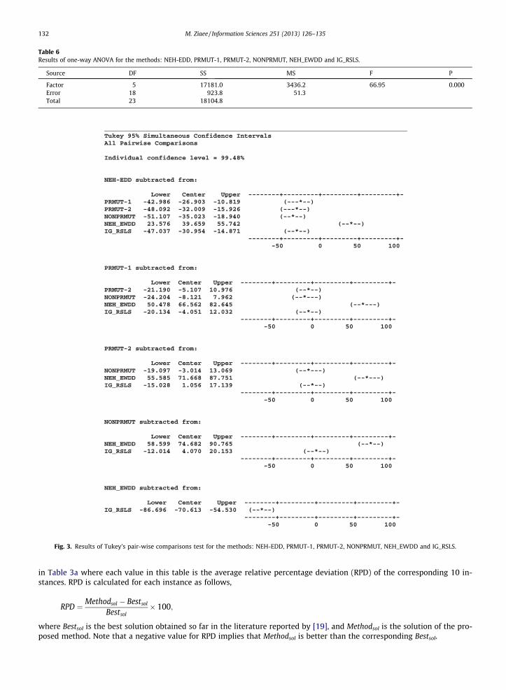
Table 6Results of one-way ANOVA for the methods: NEH-EDD, PRMUT-1, PRMUT-2, NONPRMUT, NEH_EWDD and IG_RSLS.

Source DF SS MS F P

Factor 5 17181.0 3436.2 66.95 0.000Error 18 923.8 51.3Total 23 18104.8

Fig. 3. Results of Tukey’s pair-wise comparisons test for the methods: NEH-EDD, PRMUT-1, PRMUT-2, NONPRMUT, NEH_EWDD and IG_RSLS.

132 M. Ziaee / Information Sciences 251 (2013) 126–135

in Table 3a where each value in this table is the average relative percentage deviation (RPD) of the corresponding 10 in-stances. RPD is calculated for each instance as follows,

RPD ¼ Methodsol � Bestsol

Bestsol� 100;

where Bestsol is the best solution obtained so far in the literature reported by [19], and Methodsol is the solution of the pro-posed method. Note that a negative value for RPD implies that Methodsol is better than the corresponding Bestsol.

-100

102030405060708090

SDST10 SDST50 SDST100 SDST125

Problem Set

Ave

rage

RP

D

NEH-EDD

PRMUT-1

PRMUT-2

NONPRMUT

NEH_EWDD

IG_RSLS

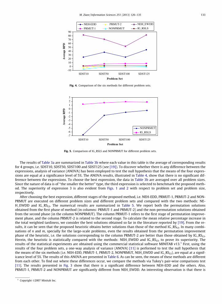
Fig. 4. Comparison of the six methods for different problem sets.

-7-6-5-4-3-2-10123

SDST10 SDST50 SDST100 SDST125

Problem Set

Ave

rage

RP

D

NONPRMUT

IG_RSLS

Fig. 5. Comparison of IG_RSLS and NONPRMUT for different problem sets.

M. Ziaee / Information Sciences 251 (2013) 126–135 133

The results of Table 3a are summarized in Table 3b where each value in this table is the average of corresponding resultsfor 4 groups, i.e. SDST10, SDST50, SDST100 and SDST125 (see [19]). To discover whether there is any difference between theexpressions, analysis of variance (ANOVA) has been employed to test the null hypothesis that the means of the four expres-sions are equal at a significance level of 5%. The ANOVA results, illustrated in Table 4, show that there is no significant dif-ference between the expressions. To choose the best expression, the data in Table 3b are averaged over all problem sizes.Since the nature of data is of ‘‘the smaller the better’’ type, the third expression is selected to benchmark the proposed meth-od. The superiority of expression 3 is also evident from Figs. 1 and 2 with respect to problem set and problem size,respectively.

After choosing the best expression, different stages of the proposed method, i.e. NEH-EDD, PRMUT-1, PRMUT-2 and NON-PRMUT are executed on different problem sizes and different problem sets and compared with the two methods: NE-H_EWDD and IG_RSLS. The numerical results are summarized in Table 5. We report both the permutation solutionsobtained from the first phase of method (in columns: PRMUT-1 and PRMUT-2) and the non-permutation solutions obtainedfrom the second phase (in the column NONPRMUT). The column PRMUT-1 refers to the first stage of permutation improve-ment phase, and the column PRMUT-2 is related to the second stage. To calculate the mean relative percentage increase inthe total weighted tardiness, we consider the best solutions obtained so far in the literature reported by [19]. From the re-sults, it can be seen that the proposed heuristic obtains better solutions than those of the method IG_RSLS. In many combi-nations of n and m, specially for the large-scale problems, even the results obtained from the permutation improvementphase of the heuristic, i.e. the solutions corresponding to the column PRMUT-2 are better than those obtained by IG_RSLS.Herein, the heuristic is statistically compared with the methods: NEH_EWDD and IG_RSLS, to prove its superiority. Theresults of the statistical experiments are obtained using the commercial statistical software MINITAB v13.1 First, using theresults of the four problem sets, a one-way analysis of variance (ANOVA) [11] is performed to test the null hypothesis thatthe means of the six methods (i.e. NEH-EDD, PRMUT-1, PRMUT-2, NONPRMUT, NEH_EWDD and IG_RSLS), are equal at a signif-icance level of 5%. The results of this ANOVA are presented in Table 6. As can be seen, the means of these methods are differentfrom each other. To find out where these differences occur, we compare the methods via Tukey’s pair-wise comparisons test[11]. The results presented in Fig. 3 show that there is a significant difference between NEH-EDD and the others. Also,PRMUT-1, PRMUT-2 and NONPRMUT are significantly different from NEH_EWDD. An interesting observation is that there is

1 Copyright �2007 Minitab Inc.

134 M. Ziaee / Information Sciences 251 (2013) 126–135

no significant difference between the means of NONPRMUT and IG_RSLS. To see the differences between the six algorithms, weinvestigate them graphically. Fig. 4 shows a graphical comparison of the average RPD of the six methods for different problemsets. The figure shows that NONPRMUT outperforms the others. Specially, NONPRMUT is significantly superior to NEH_EWDD.To clearly observe the difference between NONPRMUT and IG_RSLS, these two methods are illustrated separately in Fig. 5. As itcan be seen, in all the problem sets, NONPRMUT is better than IG_RSLS. It must be noted that Ruiz and Stutzle [19] have madeuse of a PC/AT computer with an Athlon XP 1600 + processor (1400 MHz) and 512 MBytes of main memory, while we have useda PC with a Pentium-IV 1700 MHz CPU and 512 MB RAM. Differences in the computers used for running the algorithms makethe direct comparison of computational times difficult. However, even accounting for possible relative differences in speed be-tween the processors involved, the heuristic is faster than the IG_RSLS.

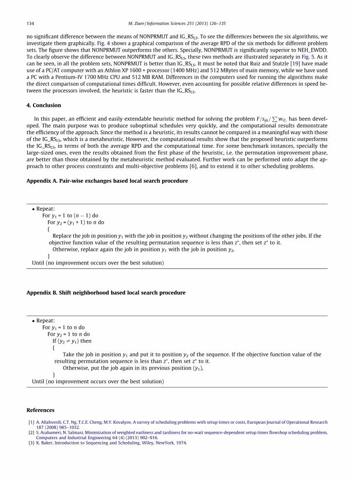
4. Conclusion

In this paper, an efficient and easily extendable heuristic method for solving the problem F=sijk=P

wiTihas been devel-

oped. The main purpose was to produce suboptimal schedules very quickly, and the computational results demonstratethe efficiency of the approach. Since the method is a heuristic, its results cannot be compared in a meaningful way with thoseof the IG_RSLS, which is a metaheuristic. However, the computational results show that the proposed heuristic outperformsthe IG_RSLS, in terms of both the average RPD and the computational time. For some benchmark instances, specially thelarge-sized ones, even the results obtained from the first phase of the heuristic, i.e. the permutation improvement phase,are better than those obtained by the metaheuristic method evaluated. Further work can be performed onto adapt the ap-proach to other process constraints and multi-objective problems [6], and to extend it to other scheduling problems.

Appendix A. Pair-wise exchanges based local search procedure

� Repeat:For y1 = 1 to (n � 1) do

For y2 = (y1 + 1) to n do{

Replace the job in position y1 with the job in position y2 without changing the positions of the other jobs. If theobjective function value of the resulting permutation sequence is less than z⁄, then set z⁄ to it.

Otherwise, replace again the job in position y1 with the job in position y2.}

Until (no improvement occurs over the best solution)

Appendix B. Shift neighborhood based local search procedure

� Repeat:For y1 = 1 to n do

For y2 = 1 to n doIf (y2 – y1) then{

Take the job in position y1 and put it to position y2 of the sequence. If the objective function value of theresulting permutation sequence is less than z⁄, then set z⁄ to it.

Otherwise, put the job again in its previous position (y1),}

Until (no improvement occurs over the best solution)

References

[1] A. Allahverdi, C.T. Ng, T.C.E. Cheng, M.Y. Kovalyov, A survey of scheduling problems with setup times or costs, European Journal of Operational Research187 (2008) 985–1032.

[2] S. Arabameri, N. Salmasi, Minimization of weighted earliness and tardiness for no-wait sequence-dependent setup times flowshop scheduling problem,Computers and Industrial Engineering 64 (4) (2013) 902–916.

[3] K. Baker, Introduction to Sequencing and Scheduling, Wiley, NewYork, 1974.

M. Ziaee / Information Sciences 251 (2013) 126–135 135

[4] T. Eren, A bicriteria m-machine flowshop scheduling with sequence-dependent setup times, Applied Mathematical Modelling 34 (2) (2010) 284–293.[5] T. Ghosh, S. Sengupta, M. Chattopadhyay, P.K. Dan, Meta-heuristics in cellular manufacturing: a state-of-the-art review, International Journal of

Industrial Engineering Computations 2 (2011) 87–122.[6] T. Khodadadzadeh, S.J. Sadjadi, A state-of-art review on supplier selection problem, Decision Science Letters 2 (2013) 59–70.[7] C. Koulamas, A new constructive heuristic for the flowshop scheduling problem, European Journal of Operational Research 105 (1998) 66–71.[8] W.-H. Kuo, C.-J. Hsu, D.-L. Yang, Worst-case and numerical analysis of heuristic algorithms for flowshop scheduling problems with a time-dependent

learning effect, Information Sciences 184 (2012) 282–297.[9] C.J. Liao, L.M. Liao, C.T. Tseng, A performance evaluation of permutation vs. non-permutation schedules in a flowshop, International Journal of

Production Research 44 (20) (2006) 4297–4309.[10] H. Matsuo, C. Suh, R. Sullivan, A controlled search simulated annealing method for the general job-shop scheduling problem, Tech. Rep. 03-04-88, Dept.

of Management, The University of Texas, Austin, 1988.[11] D.C. Montgomery, Design and Analysis of Experiments, fifth ed., John Wiley & Sons, NewYork, 2000.[12] M. Nawaz, E.E. Enscore Jr., I. Ham, A heuristic algorithm for the m-machine, n-job flowshop sequencing problem, Omega 11 (1983) 91–95.[13] Q.-K. Pan, R. Ruiz, An estimation of distribution algorithm for lot-streaming flow shop problems with setup times, Omega 40 (2) (2012) 166–180.[14] M. Pinedo, Scheduling: Theory, Algorithms and Systems, Prentice-Hall, Englewood Cliffs, NJ, 2002.[15] C.N. Potts, D.B. Shmoys, D.P. Williamson, Permutation vs. non-permutation flowshop schedules, Operations Research Letters 10 (1991) 281–284.[16] S. Pugazhendhi, S. Thiagarajan, C. Rajendran, N. Anantharaman, Performance enhancement by using non-permutation schedules in flowline-based

manufacturing systems, Computers and Industrial Engineering 44 (2002) 133–157.[17] R.Z. Rios-Mercado, J.F. Bard, Heuristics for the flow line problem with setup costs, European Journal of Operational Research 110 (1998) 76–98.[18] R. Ruiz, C. Maroto, J. Alcaraz, Solving the flowshop scheduling problem with sequence dependent setup times using advanced metaheuristics, European

Journal of Operational Research 165 (2005) 34–54.[19] R. Ruiz, T. Stutzle, An Iterated Greedy heuristic for the sequence dependent setup times flowshop problem with makespan and weighted tardiness

objectives, European Journal of Operational Research 187 (2008) 1143–1159.[20] E. Taillard, Benchmarks for basic scheduling problems, European Journal of Operational Research 64 (1993) 278–285.[21] H.A. Tahmasbi, R. Tavakkoli-Moghaddam, Solving a bi-objective flowshop scheduling problem by a multi-objective immune system and comparing

with SPEA2+ and SPGA, Advances in Engineering Software 42 (10) (2011) 772–779.[22] M. Tandon, P.T. Cummings, M.D. LeVan, Flowshop sequencing with non-permutation schedules, Computers and Chemical Engineering 15 (1991) 601–

607.[23] F.T. Tseng, J.N.D. Gupta, E.F. Stafford, A penalty-based heuristic algorithm for the permutation flowshop scheduling problem with sequence-dependent

set-up times, Journal of the Operational Research Society 57 (2006) 541–551.[24] K.-C. Ying, Solving non-permutation flowshop scheduling problems by an effective iterated greedy heuristic, International Journal of Advanced

Manufacturing Technology 38 (2008) 348–354.