Embed Size (px)
Citation preview
General Linear ModelsGeneralized Linear Models
Hal Whitehead
BIOL40625062
bull Transformations
bull Analysis of Covariance
bull General Linear Models
bull Generalized Linear Models
bull Non-Linear Models
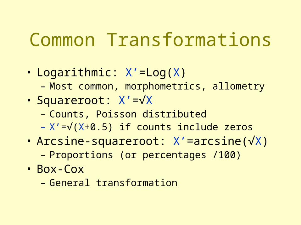
Common Transformations
bull Logarithmic Xrsquo=Log(X)ndash Most common morphometrics allometry
bull Squareroot Xrsquo=radicXndash Counts Poisson distributedndash Xrsquo=radic(X+05) if counts include zeros
bull Arcsine-squareroot Xrsquo=arcsine(radicX)ndash Proportions (or percentages 100)
bull Box-Coxndash General transformation
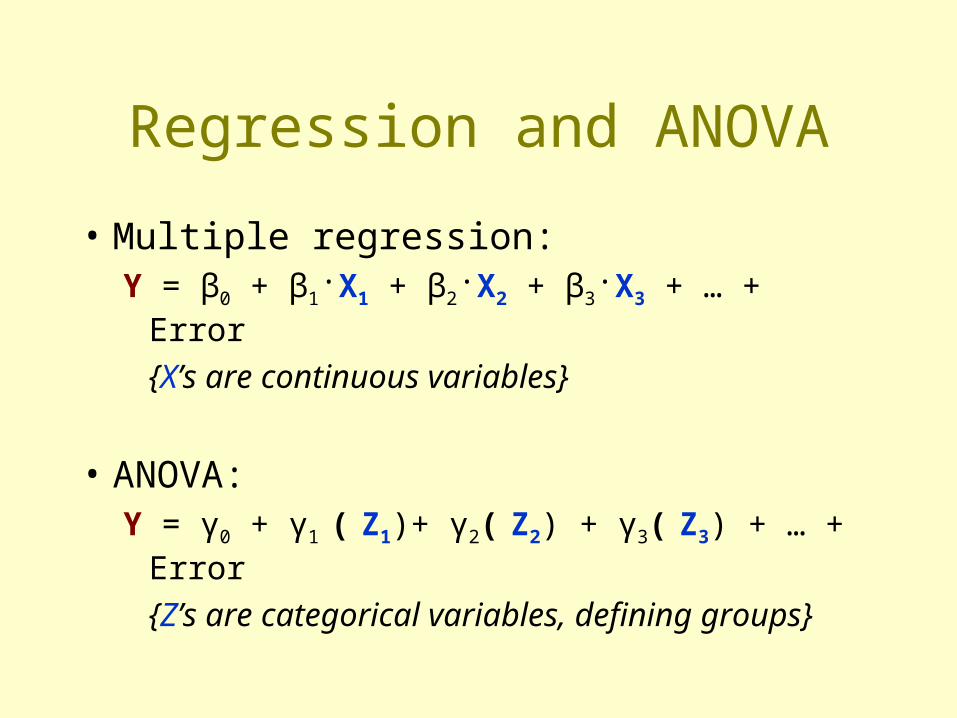
Regression and ANOVA
bull Multiple regressionY = β0 + β1X1 + β2X2 + β3X3 + hellip + Error
Xrsquos are continuous variables
bull ANOVAY = γ0 + γ1 ( Z1)+ γ2( Z2) + γ3( Z3) + hellip + Error
Zrsquos are categorical variables defining groups
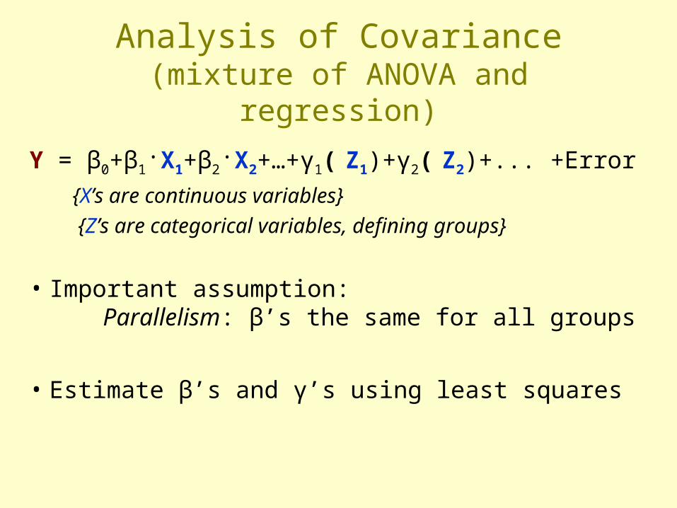
Analysis of Covariance(mixture of ANOVA and regression)
Y = β0+β1X1+β2X2+hellip+γ1( Z1)+γ2( Z2)+ +Error
Xrsquos are continuous variables
Zrsquos are categorical variables defining groups
bull Important assumptionParallelism βrsquos the same for all groups
bull Estimate βrsquos and γrsquos using least squares
Analysis of Covariance
bull Datandash Catch rates of sperm whales (per whaling day) by
Yankee whalers from logbooks of Yankee whalers off Galapagos Islands 1830-1850
bull Questionsndash Was there a significant change in catch rate over this
period
ndash Was there a significant seasonal pattern
Analysis of Covariance
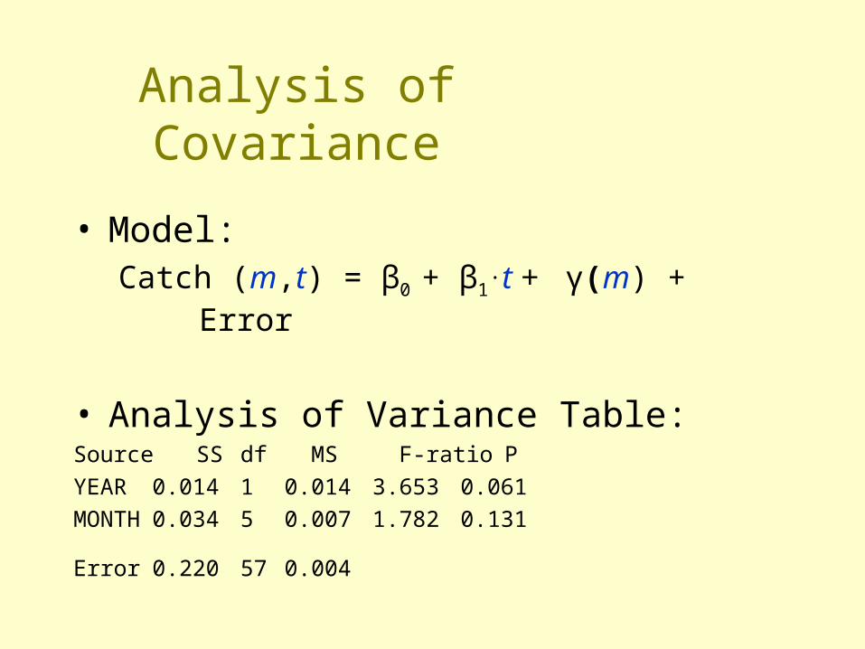
bull ModelCatch (mt) = β0 + β1t + γ(m) + Error
t =1830-1850 [continuous]
m = Jan-Feb Mar-Apr hellip Nov-Dec
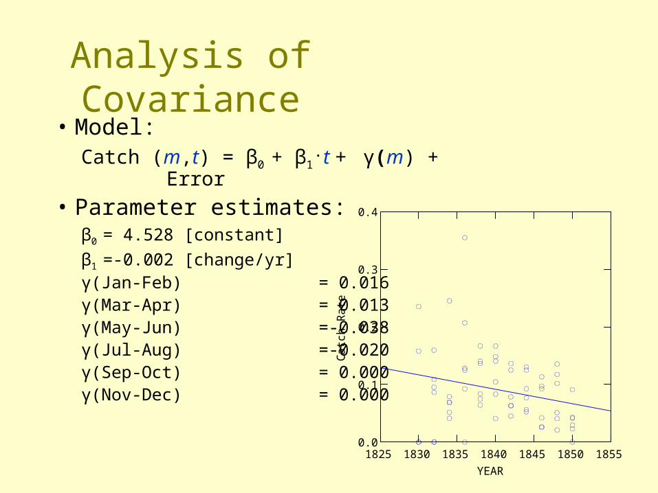
Analysis of Covariancebull Model
Catch (mt) = β0 + β1t + γ(m) + Error
bull Parameter estimatesβ0 = 4528 [constant]
β1 =-0002 [changeyr]γ(Jan-Feb) = 0016γ(Mar-Apr) = 0013γ(May-Jun) =-0038γ(Jul-Aug) =-0020γ(Sep-Oct) = 0000γ(Nov-Dec) = 0000
1825 1830 1835 1840 1845 1850 1855YEAR
00
01
02
03
04
Ca
tch
Ra
te
Analysis of Covariance
bull ModelCatch (mt) = β0 + β1t + γ(m) + Error
bull Analysis of Variance TableSource SS df MS F-ratio P
YEAR 0014 1 0014 3653 0061
MONTH 0034 5 0007 1782 0131
Error 0220 57 0004
Analysis of Covariance
Plot of Residuals against Predicted Values
006 007 008 009 010 011 012 013Estimated Catch Rate
-02
-01
00
01
02
03
RE
SID
UA
L
Durbin-Watson D Statistic 1923First Order Autocorrelation 0034
General Linear ModelAnalysis of Covariance plus Interactions
Y = β0 + β1X1 + β2X2 + hellip
+ γ1 ( Z1) + γ2 ( Z2) + hellip
+ β12X1X2 + hellip
+ γ12 ( Z1 Z2) + hellip
+ α12 ( Z1)X1 + hellip
+ ErrorXrsquos are continuous variables
Zrsquos are categorical variables defining groups
Characteristics of General Linear Models
bull The response Y has a normal distribution with vector mean μ and SD σ2
bull A coefficient vector (b=[βrsquos γrsquos αrsquos]) defines a linear combination of the predictors (Xrsquos)
bull The model equates the two as
μ = Xb
General Linear Models
bull Coefficients (βrsquos γrsquos αrsquos) and fit of model (σsup2 or rsup2) estimated using least squares
bull Subsets of predictor variables may be selected using stepwise methods etc
bull Bewarendash Collinearityndash Empty or nearly-empty cells (combinations of
categorical variables with few units)
General Linear Model
bull Datandash Movements of sperm whales (displacement per
12-hr) off Galapagos Islands with year clan and shit rate
bull Questionsndash Are movements of sperm whales affected by year
clan shit rate or combinations of them
General Linear Model
Potential X variablesYear (Categorical 1987 and 1989)Clan (Categorical lsquoPlus-onersquo and lsquoRegularrsquo)Shit-rate (Continuous Arcsine-Squareroot transform)YearClanYearShit-rateClanShit-rate
General Linear Model
X variables selected by stepwise selection (P-to-enter = 015 P-to-remove = 015)
Backward ForwardYear Year
Clan Clan
Shit-rate Shit-rate
YearClan YearClan
YearShit-rate YearShit-rate
ClanShit-rate ClanShit-rate
General Linear Model
bull BackwardY =c + Clan + YearClan
bull ForwardY =c + Shit-rateClan
1987 1989YEAR
0
10
20
30
40
50
60
12-h
r D
ispl
acem
ent (
km)
Reg+1
CL
01 02 03 04 05 06 07 08 09Shit rate (transformed)
0
10
20
30
40
50
60
12-h
r D
ispl
acem
ent (
km)
Reg+1
CL
General Linear Model
Why two ldquobest modelsrdquo
bull BackwardY =c + Clan + YearClan
bull ForwardY =c + Shit-rateClan
1987 1989YEAR
0
10
20
30
40
50
60
12-h
r D
ispl
acem
ent (
km)
Reg+1
CL
01 02 03 04 05 06 07 08 09Shit rate (transformed)
0
10
20
30
40
50
60
12-h
r D
ispl
acem
ent (
km)
Reg+1
CL
1987 1989
General Linear Model
Which is ldquobestrdquo
bull BackwardY =c + Clan + YearClan
bull ForwardY =c + Shit-rateClan
1987 1989YEAR
0
10
20
30
40
50
60
12-h
r D
ispl
acem
ent (
km)
Reg+1
CL
01 02 03 04 05 06 07 08 09Shit rate (transformed)
0
10
20
30
40
50
60
12-h
r D
ispl
acem
ent (
km)
Reg+1
CL
1987 1989
rsup2=02642 df
rsup2=03471 df
General Linear Models
bull The response Y has a normal distribution with vector mean μ and SD σ2
bull A coefficient vector (b=[βrsquos γrsquos αrsquos]) defines a linear combination of the predictors (Xrsquos)
bull The model equates the two as
μ = Xb
Generalized Linear Modelsbull The response Y has a distribution that may be
normal binomial Poisson gamma or inverse Gaussian with parameters including a mean micro
bull A coefficient vector (b=[βrsquos γrsquos αrsquos]) defines a linear combination of the predictors (Xrsquos)
bull A link function f defines the link between the two as
f(μ) = Xb
Generalized linear models
bull Examine assumptions using residuals
bull Examine fit using ldquodeviancerdquondash a generalization of the residual sum of squaresndash twice difference of log-likelihoods of model in
question and full modelndash fits of different models can be compared ndash Related to AIC
-1 0 1 20
05
1Logistic function
90 91 92 93 94 95 96 97 98 991000
10
20
30
40Binomial distribution
05 1 15 205
1
15
2Reciprocal function
0 1 2 3 4 5 6 7 8 9 100
10
20
30Poisson distribution
Generalized Linear Modelscan fit non-linear relationships using
lsquolink functionsrsquo and can consider non-normal errors
MATLAB glmdemo
Proportion of sexually-mature animals at different weights
2000 2500 3000 3500 4000 45000
01
02
03
04
05
06
07
08
09
1
Weight
Pro
port
ion
MATLAB glmdemo
Two problems with linear regression1) probabilities lt0 and gt1
2) clearly non-linear
2000 2500 3000 3500 4000 4500-02
0
02
04
06
08
1
12
Weight
Pro
port
ion
MATLAB glmdemo
Polynomial Regression better but also
1) probabilities lt0 and gt1
2) inflections are not real
2000 2500 3000 3500 4000 4500-02
0
02
04
06
08
1
12
Weight
Pro
port
ion
MATLAB glmdemo
Instead fit ldquologistic regressionrdquousing generalized linear model and
binomial distribution
MATLAB glmdemo
2000 2500 3000 3500 4000 45000
01
02
03
04
05
06
07
08
09
1
Weight
Pro
port
ion
sexu
ally
mat
ure
Y= 1(1+e β0+β1X)
2000 2500 3000 3500 4000 45000
01
02
03
04
05
06
07
08
09
1
Weight
Pro
port
ion
sexu
ally
mat
ure
Compare two generalized linear models
MATLAB glmdemo
Y= 1(1+e β0+β1X)
Y= 1(1+e β0+β1X +β2XX)
Difference in deviance =070 P=040
Examine assumptions using residuals
-1 -05 0 05 1
005
010
025
050
075
090
095
Data
Pro
babi
lity
Normal Probability Plot
MATLAB glmdemo
Making predictions
2400 2600 2800 3000 3200 3400 3600 3800 4000 42000
10
20
30
40
50
60
70
80
90
100
Weight
Pro
babi
lity
sexu
ally
mat
ure
MATLAB glmdemo
Non-linear models eg
Y = c + EXP(szlig0 + szlig1X) + E
Y = szlig0 + szlig1X[XgtXK] + Ebull More general than generalized linear
models
bull But harder to fitndash iterative processndash may not convergendash non-unique solutionndash harder to compare
SummaryMethods with One Dependent
Variable Simple Linear Regression One-way ANOVA
Multiple Linear Regression Multi-way ANOVA
Analysis of Covariance
General Linear Model
Generalized Linear Model
Non-Linear Model
IncreasingComplexity
bull Transformations
bull Analysis of Covariance
bull General Linear Models
bull Generalized Linear Models
bull Non-Linear Models
Common Transformations
bull Logarithmic Xrsquo=Log(X)ndash Most common morphometrics allometry
bull Squareroot Xrsquo=radicXndash Counts Poisson distributedndash Xrsquo=radic(X+05) if counts include zeros
bull Arcsine-squareroot Xrsquo=arcsine(radicX)ndash Proportions (or percentages 100)
bull Box-Coxndash General transformation
Regression and ANOVA
bull Multiple regressionY = β0 + β1X1 + β2X2 + β3X3 + hellip + Error
Xrsquos are continuous variables
bull ANOVAY = γ0 + γ1 ( Z1)+ γ2( Z2) + γ3( Z3) + hellip + Error
Zrsquos are categorical variables defining groups
Analysis of Covariance(mixture of ANOVA and regression)
Y = β0+β1X1+β2X2+hellip+γ1( Z1)+γ2( Z2)+ +Error
Xrsquos are continuous variables
Zrsquos are categorical variables defining groups
bull Important assumptionParallelism βrsquos the same for all groups
bull Estimate βrsquos and γrsquos using least squares
Analysis of Covariance
bull Datandash Catch rates of sperm whales (per whaling day) by
Yankee whalers from logbooks of Yankee whalers off Galapagos Islands 1830-1850
bull Questionsndash Was there a significant change in catch rate over this
period
ndash Was there a significant seasonal pattern
Analysis of Covariance
bull ModelCatch (mt) = β0 + β1t + γ(m) + Error
t =1830-1850 [continuous]
m = Jan-Feb Mar-Apr hellip Nov-Dec
Analysis of Covariancebull Model
Catch (mt) = β0 + β1t + γ(m) + Error
bull Parameter estimatesβ0 = 4528 [constant]
β1 =-0002 [changeyr]γ(Jan-Feb) = 0016γ(Mar-Apr) = 0013γ(May-Jun) =-0038γ(Jul-Aug) =-0020γ(Sep-Oct) = 0000γ(Nov-Dec) = 0000
1825 1830 1835 1840 1845 1850 1855YEAR
00
01
02
03
04
Ca
tch
Ra
te
Analysis of Covariance
bull ModelCatch (mt) = β0 + β1t + γ(m) + Error
bull Analysis of Variance TableSource SS df MS F-ratio P
YEAR 0014 1 0014 3653 0061
MONTH 0034 5 0007 1782 0131
Error 0220 57 0004
Analysis of Covariance
Plot of Residuals against Predicted Values
006 007 008 009 010 011 012 013Estimated Catch Rate
-02
-01
00
01
02
03
RE
SID
UA
L
Durbin-Watson D Statistic 1923First Order Autocorrelation 0034
General Linear ModelAnalysis of Covariance plus Interactions
Y = β0 + β1X1 + β2X2 + hellip
+ γ1 ( Z1) + γ2 ( Z2) + hellip
+ β12X1X2 + hellip
+ γ12 ( Z1 Z2) + hellip
+ α12 ( Z1)X1 + hellip
+ ErrorXrsquos are continuous variables
Zrsquos are categorical variables defining groups
Characteristics of General Linear Models
bull The response Y has a normal distribution with vector mean μ and SD σ2
bull A coefficient vector (b=[βrsquos γrsquos αrsquos]) defines a linear combination of the predictors (Xrsquos)
bull The model equates the two as
μ = Xb
General Linear Models
bull Coefficients (βrsquos γrsquos αrsquos) and fit of model (σsup2 or rsup2) estimated using least squares
bull Subsets of predictor variables may be selected using stepwise methods etc
bull Bewarendash Collinearityndash Empty or nearly-empty cells (combinations of
categorical variables with few units)
General Linear Model
bull Datandash Movements of sperm whales (displacement per
12-hr) off Galapagos Islands with year clan and shit rate
bull Questionsndash Are movements of sperm whales affected by year
clan shit rate or combinations of them
General Linear Model
Potential X variablesYear (Categorical 1987 and 1989)Clan (Categorical lsquoPlus-onersquo and lsquoRegularrsquo)Shit-rate (Continuous Arcsine-Squareroot transform)YearClanYearShit-rateClanShit-rate
General Linear Model
X variables selected by stepwise selection (P-to-enter = 015 P-to-remove = 015)
Backward ForwardYear Year
Clan Clan
Shit-rate Shit-rate
YearClan YearClan
YearShit-rate YearShit-rate
ClanShit-rate ClanShit-rate
General Linear Model
bull BackwardY =c + Clan + YearClan
bull ForwardY =c + Shit-rateClan
1987 1989YEAR
0
10
20
30
40
50
60
12-h
r D
ispl
acem
ent (
km)
Reg+1
CL
01 02 03 04 05 06 07 08 09Shit rate (transformed)
0
10
20
30
40
50
60
12-h
r D
ispl
acem
ent (
km)
Reg+1
CL
General Linear Model
Why two ldquobest modelsrdquo
bull BackwardY =c + Clan + YearClan
bull ForwardY =c + Shit-rateClan
1987 1989YEAR
0
10
20
30
40
50
60
12-h
r D
ispl
acem
ent (
km)
Reg+1
CL
01 02 03 04 05 06 07 08 09Shit rate (transformed)
0
10
20
30
40
50
60
12-h
r D
ispl
acem
ent (
km)
Reg+1
CL
1987 1989
General Linear Model
Which is ldquobestrdquo
bull BackwardY =c + Clan + YearClan
bull ForwardY =c + Shit-rateClan
1987 1989YEAR
0
10
20
30
40
50
60
12-h
r D
ispl
acem
ent (
km)
Reg+1
CL
01 02 03 04 05 06 07 08 09Shit rate (transformed)
0
10
20
30
40
50
60
12-h
r D
ispl
acem
ent (
km)
Reg+1
CL
1987 1989
rsup2=02642 df
rsup2=03471 df
General Linear Models
bull The response Y has a normal distribution with vector mean μ and SD σ2
bull A coefficient vector (b=[βrsquos γrsquos αrsquos]) defines a linear combination of the predictors (Xrsquos)
bull The model equates the two as
μ = Xb
Generalized Linear Modelsbull The response Y has a distribution that may be
normal binomial Poisson gamma or inverse Gaussian with parameters including a mean micro
bull A coefficient vector (b=[βrsquos γrsquos αrsquos]) defines a linear combination of the predictors (Xrsquos)
bull A link function f defines the link between the two as
f(μ) = Xb
Generalized linear models
bull Examine assumptions using residuals
bull Examine fit using ldquodeviancerdquondash a generalization of the residual sum of squaresndash twice difference of log-likelihoods of model in
question and full modelndash fits of different models can be compared ndash Related to AIC
-1 0 1 20
05
1Logistic function
90 91 92 93 94 95 96 97 98 991000
10
20
30
40Binomial distribution
05 1 15 205
1
15
2Reciprocal function
0 1 2 3 4 5 6 7 8 9 100
10
20
30Poisson distribution
Generalized Linear Modelscan fit non-linear relationships using
lsquolink functionsrsquo and can consider non-normal errors
MATLAB glmdemo
Proportion of sexually-mature animals at different weights
2000 2500 3000 3500 4000 45000
01
02
03
04
05
06
07
08
09
1
Weight
Pro
port
ion
MATLAB glmdemo
Two problems with linear regression1) probabilities lt0 and gt1
2) clearly non-linear
2000 2500 3000 3500 4000 4500-02
0
02
04
06
08
1
12
Weight
Pro
port
ion
MATLAB glmdemo
Polynomial Regression better but also
1) probabilities lt0 and gt1
2) inflections are not real
2000 2500 3000 3500 4000 4500-02
0
02
04
06
08
1
12
Weight
Pro
port
ion
MATLAB glmdemo
Instead fit ldquologistic regressionrdquousing generalized linear model and
binomial distribution
MATLAB glmdemo
2000 2500 3000 3500 4000 45000
01
02
03
04
05
06
07
08
09
1
Weight
Pro
port
ion
sexu
ally
mat
ure
Y= 1(1+e β0+β1X)
2000 2500 3000 3500 4000 45000
01
02
03
04
05
06
07
08
09
1
Weight
Pro
port
ion
sexu
ally
mat
ure
Compare two generalized linear models
MATLAB glmdemo
Y= 1(1+e β0+β1X)
Y= 1(1+e β0+β1X +β2XX)
Difference in deviance =070 P=040
Examine assumptions using residuals
-1 -05 0 05 1
005
010
025
050
075
090
095
Data
Pro
babi
lity
Normal Probability Plot
MATLAB glmdemo
Making predictions
2400 2600 2800 3000 3200 3400 3600 3800 4000 42000
10
20
30
40
50
60
70
80
90
100
Weight
Pro
babi
lity
sexu
ally
mat
ure
MATLAB glmdemo
Non-linear models eg
Y = c + EXP(szlig0 + szlig1X) + E
Y = szlig0 + szlig1X[XgtXK] + Ebull More general than generalized linear
models
bull But harder to fitndash iterative processndash may not convergendash non-unique solutionndash harder to compare
SummaryMethods with One Dependent
Variable Simple Linear Regression One-way ANOVA
Multiple Linear Regression Multi-way ANOVA
Analysis of Covariance
General Linear Model
Generalized Linear Model
Non-Linear Model
IncreasingComplexity
Analysis of Covariance
bull ModelCatch (mt) = β0 + β1t + γ(m) + Error
t =1830-1850 [continuous]
m = Jan-Feb Mar-Apr hellip Nov-Dec
Analysis of Covariancebull Model
Catch (mt) = β0 + β1t + γ(m) + Error
bull Parameter estimatesβ0 = 4528 [constant]
β1 =-0002 [changeyr]γ(Jan-Feb) = 0016γ(Mar-Apr) = 0013γ(May-Jun) =-0038γ(Jul-Aug) =-0020γ(Sep-Oct) = 0000γ(Nov-Dec) = 0000
1825 1830 1835 1840 1845 1850 1855YEAR
00
01
02
03
04
Ca
tch
Ra
te
Analysis of Covariance
bull ModelCatch (mt) = β0 + β1t + γ(m) + Error
bull Analysis of Variance TableSource SS df MS F-ratio P
YEAR 0014 1 0014 3653 0061
MONTH 0034 5 0007 1782 0131
Error 0220 57 0004
Analysis of Covariance
Plot of Residuals against Predicted Values
006 007 008 009 010 011 012 013Estimated Catch Rate
-02
-01
00
01
02
03
RE
SID
UA
L
Durbin-Watson D Statistic 1923First Order Autocorrelation 0034
General Linear ModelAnalysis of Covariance plus Interactions
Y = β0 + β1X1 + β2X2 + hellip
+ γ1 ( Z1) + γ2 ( Z2) + hellip
+ β12X1X2 + hellip
+ γ12 ( Z1 Z2) + hellip
+ α12 ( Z1)X1 + hellip
+ ErrorXrsquos are continuous variables
Zrsquos are categorical variables defining groups
Characteristics of General Linear Models
bull The response Y has a normal distribution with vector mean μ and SD σ2
bull A coefficient vector (b=[βrsquos γrsquos αrsquos]) defines a linear combination of the predictors (Xrsquos)
bull The model equates the two as
μ = Xb
General Linear Models
bull Coefficients (βrsquos γrsquos αrsquos) and fit of model (σsup2 or rsup2) estimated using least squares
bull Subsets of predictor variables may be selected using stepwise methods etc
bull Bewarendash Collinearityndash Empty or nearly-empty cells (combinations of
categorical variables with few units)
General Linear Model
bull Datandash Movements of sperm whales (displacement per
12-hr) off Galapagos Islands with year clan and shit rate
bull Questionsndash Are movements of sperm whales affected by year
clan shit rate or combinations of them
General Linear Model
Potential X variablesYear (Categorical 1987 and 1989)Clan (Categorical lsquoPlus-onersquo and lsquoRegularrsquo)Shit-rate (Continuous Arcsine-Squareroot transform)YearClanYearShit-rateClanShit-rate
General Linear Model
X variables selected by stepwise selection (P-to-enter = 015 P-to-remove = 015)
Backward ForwardYear Year
Clan Clan
Shit-rate Shit-rate
YearClan YearClan
YearShit-rate YearShit-rate
ClanShit-rate ClanShit-rate
General Linear Model
bull BackwardY =c + Clan + YearClan
bull ForwardY =c + Shit-rateClan
1987 1989YEAR
0
10
20
30
40
50
60
12-h
r D
ispl
acem
ent (
km)
Reg+1
CL
01 02 03 04 05 06 07 08 09Shit rate (transformed)
0
10
20
30
40
50
60
12-h
r D
ispl
acem
ent (
km)
Reg+1
CL
General Linear Model
Why two ldquobest modelsrdquo
bull BackwardY =c + Clan + YearClan
bull ForwardY =c + Shit-rateClan
1987 1989YEAR
0
10
20
30
40
50
60
12-h
r D
ispl
acem
ent (
km)
Reg+1
CL
01 02 03 04 05 06 07 08 09Shit rate (transformed)
0
10
20
30
40
50
60
12-h
r D
ispl
acem
ent (
km)
Reg+1
CL
1987 1989
General Linear Model
Which is ldquobestrdquo
bull BackwardY =c + Clan + YearClan
bull ForwardY =c + Shit-rateClan
1987 1989YEAR
0
10
20
30
40
50
60
12-h
r D
ispl
acem
ent (
km)
Reg+1
CL
01 02 03 04 05 06 07 08 09Shit rate (transformed)
0
10
20
30
40
50
60
12-h
r D
ispl
acem
ent (
km)
Reg+1
CL
1987 1989
rsup2=02642 df
rsup2=03471 df
General Linear Models
bull The response Y has a normal distribution with vector mean μ and SD σ2
bull A coefficient vector (b=[βrsquos γrsquos αrsquos]) defines a linear combination of the predictors (Xrsquos)
bull The model equates the two as
μ = Xb
Generalized Linear Modelsbull The response Y has a distribution that may be
normal binomial Poisson gamma or inverse Gaussian with parameters including a mean micro
bull A coefficient vector (b=[βrsquos γrsquos αrsquos]) defines a linear combination of the predictors (Xrsquos)
bull A link function f defines the link between the two as
f(μ) = Xb
Generalized linear models
bull Examine assumptions using residuals
bull Examine fit using ldquodeviancerdquondash a generalization of the residual sum of squaresndash twice difference of log-likelihoods of model in
question and full modelndash fits of different models can be compared ndash Related to AIC
-1 0 1 20
05
1Logistic function
90 91 92 93 94 95 96 97 98 991000
10
20
30
40Binomial distribution
05 1 15 205
1
15
2Reciprocal function
0 1 2 3 4 5 6 7 8 9 100
10
20
30Poisson distribution
Generalized Linear Modelscan fit non-linear relationships using
lsquolink functionsrsquo and can consider non-normal errors
MATLAB glmdemo
Proportion of sexually-mature animals at different weights
2000 2500 3000 3500 4000 45000
01
02
03
04
05
06
07
08
09
1
Weight
Pro
port
ion
MATLAB glmdemo
Two problems with linear regression1) probabilities lt0 and gt1
2) clearly non-linear
2000 2500 3000 3500 4000 4500-02
0
02
04
06
08
1
12
Weight
Pro
port
ion
MATLAB glmdemo
Polynomial Regression better but also
1) probabilities lt0 and gt1
2) inflections are not real
2000 2500 3000 3500 4000 4500-02
0
02
04
06
08
1
12
Weight
Pro
port
ion
MATLAB glmdemo
Instead fit ldquologistic regressionrdquousing generalized linear model and
binomial distribution
MATLAB glmdemo
2000 2500 3000 3500 4000 45000
01
02
03
04
05
06
07
08
09
1
Weight
Pro
port
ion
sexu
ally
mat
ure
Y= 1(1+e β0+β1X)
2000 2500 3000 3500 4000 45000
01
02
03
04
05
06
07
08
09
1
Weight
Pro
port
ion
sexu
ally
mat
ure
Compare two generalized linear models
MATLAB glmdemo
Y= 1(1+e β0+β1X)
Y= 1(1+e β0+β1X +β2XX)
Difference in deviance =070 P=040
Examine assumptions using residuals
-1 -05 0 05 1
005
010
025
050
075
090
095
Data
Pro
babi
lity
Normal Probability Plot
MATLAB glmdemo
Making predictions
2400 2600 2800 3000 3200 3400 3600 3800 4000 42000
10
20
30
40
50
60
70
80
90
100
Weight
Pro
babi
lity
sexu
ally
mat
ure
MATLAB glmdemo
Non-linear models eg
Y = c + EXP(szlig0 + szlig1X) + E
Y = szlig0 + szlig1X[XgtXK] + Ebull More general than generalized linear
models
bull But harder to fitndash iterative processndash may not convergendash non-unique solutionndash harder to compare
SummaryMethods with One Dependent
Variable Simple Linear Regression One-way ANOVA
Multiple Linear Regression Multi-way ANOVA
Analysis of Covariance
General Linear Model
Generalized Linear Model
Non-Linear Model
IncreasingComplexity
Analysis of Covariance
bull ModelCatch (mt) = β0 + β1t + γ(m) + Error
bull Analysis of Variance TableSource SS df MS F-ratio P
YEAR 0014 1 0014 3653 0061
MONTH 0034 5 0007 1782 0131
Error 0220 57 0004
Analysis of Covariance
Plot of Residuals against Predicted Values
006 007 008 009 010 011 012 013Estimated Catch Rate
-02
-01
00
01
02
03
RE
SID
UA
L
Durbin-Watson D Statistic 1923First Order Autocorrelation 0034
General Linear ModelAnalysis of Covariance plus Interactions
Y = β0 + β1X1 + β2X2 + hellip
+ γ1 ( Z1) + γ2 ( Z2) + hellip
+ β12X1X2 + hellip
+ γ12 ( Z1 Z2) + hellip
+ α12 ( Z1)X1 + hellip
+ ErrorXrsquos are continuous variables
Zrsquos are categorical variables defining groups
Characteristics of General Linear Models
bull The response Y has a normal distribution with vector mean μ and SD σ2
bull A coefficient vector (b=[βrsquos γrsquos αrsquos]) defines a linear combination of the predictors (Xrsquos)
bull The model equates the two as
μ = Xb
General Linear Models
bull Coefficients (βrsquos γrsquos αrsquos) and fit of model (σsup2 or rsup2) estimated using least squares
bull Subsets of predictor variables may be selected using stepwise methods etc
bull Bewarendash Collinearityndash Empty or nearly-empty cells (combinations of
categorical variables with few units)
General Linear Model
bull Datandash Movements of sperm whales (displacement per
12-hr) off Galapagos Islands with year clan and shit rate
bull Questionsndash Are movements of sperm whales affected by year
clan shit rate or combinations of them
General Linear Model
Potential X variablesYear (Categorical 1987 and 1989)Clan (Categorical lsquoPlus-onersquo and lsquoRegularrsquo)Shit-rate (Continuous Arcsine-Squareroot transform)YearClanYearShit-rateClanShit-rate
General Linear Model
X variables selected by stepwise selection (P-to-enter = 015 P-to-remove = 015)
Backward ForwardYear Year
Clan Clan
Shit-rate Shit-rate
YearClan YearClan
YearShit-rate YearShit-rate
ClanShit-rate ClanShit-rate
General Linear Model
bull BackwardY =c + Clan + YearClan
bull ForwardY =c + Shit-rateClan
1987 1989YEAR
0
10
20
30
40
50
60
12-h
r D
ispl
acem
ent (
km)
Reg+1
CL
01 02 03 04 05 06 07 08 09Shit rate (transformed)
0
10
20
30
40
50
60
12-h
r D
ispl
acem
ent (
km)
Reg+1
CL
General Linear Model
Why two ldquobest modelsrdquo
bull BackwardY =c + Clan + YearClan
bull ForwardY =c + Shit-rateClan
1987 1989YEAR
0
10
20
30
40
50
60
12-h
r D
ispl
acem
ent (
km)
Reg+1
CL
01 02 03 04 05 06 07 08 09Shit rate (transformed)
0
10
20
30
40
50
60
12-h
r D
ispl
acem
ent (
km)
Reg+1
CL
1987 1989
General Linear Model
Which is ldquobestrdquo
bull BackwardY =c + Clan + YearClan
bull ForwardY =c + Shit-rateClan
1987 1989YEAR
0
10
20
30
40
50
60
12-h
r D
ispl
acem
ent (
km)
Reg+1
CL
01 02 03 04 05 06 07 08 09Shit rate (transformed)
0
10
20
30
40
50
60
12-h
r D
ispl
acem
ent (
km)
Reg+1
CL
1987 1989
rsup2=02642 df
rsup2=03471 df
General Linear Models
bull The response Y has a normal distribution with vector mean μ and SD σ2
bull A coefficient vector (b=[βrsquos γrsquos αrsquos]) defines a linear combination of the predictors (Xrsquos)
bull The model equates the two as
μ = Xb
Generalized Linear Modelsbull The response Y has a distribution that may be
normal binomial Poisson gamma or inverse Gaussian with parameters including a mean micro
bull A coefficient vector (b=[βrsquos γrsquos αrsquos]) defines a linear combination of the predictors (Xrsquos)
bull A link function f defines the link between the two as
f(μ) = Xb
Generalized linear models
bull Examine assumptions using residuals
bull Examine fit using ldquodeviancerdquondash a generalization of the residual sum of squaresndash twice difference of log-likelihoods of model in
question and full modelndash fits of different models can be compared ndash Related to AIC
-1 0 1 20
05
1Logistic function
90 91 92 93 94 95 96 97 98 991000
10
20
30
40Binomial distribution
05 1 15 205
1
15
2Reciprocal function
0 1 2 3 4 5 6 7 8 9 100
10
20
30Poisson distribution
Generalized Linear Modelscan fit non-linear relationships using
lsquolink functionsrsquo and can consider non-normal errors
MATLAB glmdemo
Proportion of sexually-mature animals at different weights
2000 2500 3000 3500 4000 45000
01
02
03
04
05
06
07
08
09
1
Weight
Pro
port
ion
MATLAB glmdemo
Two problems with linear regression1) probabilities lt0 and gt1
2) clearly non-linear
2000 2500 3000 3500 4000 4500-02
0
02
04
06
08
1
12
Weight
Pro
port
ion
MATLAB glmdemo
Polynomial Regression better but also
1) probabilities lt0 and gt1
2) inflections are not real
2000 2500 3000 3500 4000 4500-02
0
02
04
06
08
1
12
Weight
Pro
port
ion
MATLAB glmdemo
Instead fit ldquologistic regressionrdquousing generalized linear model and
binomial distribution
MATLAB glmdemo
2000 2500 3000 3500 4000 45000
01
02
03
04
05
06
07
08
09
1
Weight
Pro
port
ion
sexu
ally
mat
ure
Y= 1(1+e β0+β1X)
2000 2500 3000 3500 4000 45000
01
02
03
04
05
06
07
08
09
1
Weight
Pro
port
ion
sexu
ally
mat
ure
Compare two generalized linear models
MATLAB glmdemo
Y= 1(1+e β0+β1X)
Y= 1(1+e β0+β1X +β2XX)
Difference in deviance =070 P=040
Examine assumptions using residuals
-1 -05 0 05 1
005
010
025
050
075
090
095
Data
Pro
babi
lity
Normal Probability Plot
MATLAB glmdemo
Making predictions
2400 2600 2800 3000 3200 3400 3600 3800 4000 42000
10
20
30
40
50
60
70
80
90
100
Weight
Pro
babi
lity
sexu
ally
mat
ure
MATLAB glmdemo
Non-linear models eg
Y = c + EXP(szlig0 + szlig1X) + E
Y = szlig0 + szlig1X[XgtXK] + Ebull More general than generalized linear
models
bull But harder to fitndash iterative processndash may not convergendash non-unique solutionndash harder to compare
SummaryMethods with One Dependent
Variable Simple Linear Regression One-way ANOVA
Multiple Linear Regression Multi-way ANOVA
Analysis of Covariance
General Linear Model
Generalized Linear Model
Non-Linear Model
IncreasingComplexity
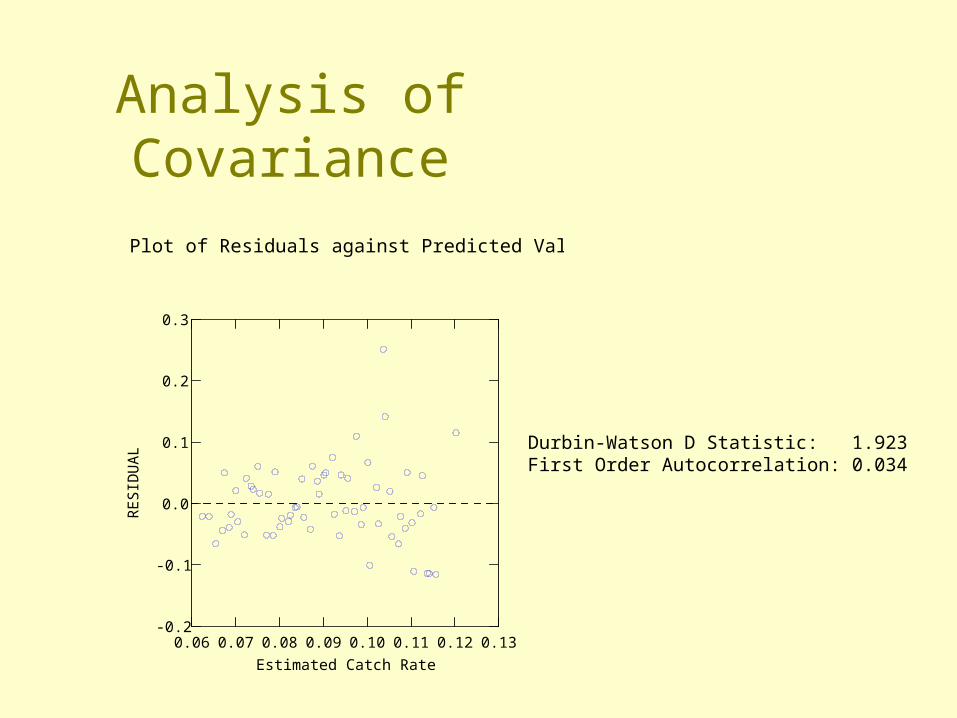
Analysis of Covariance
Plot of Residuals against Predicted Values
006 007 008 009 010 011 012 013Estimated Catch Rate
-02
-01
00
01
02
03
RE
SID
UA
L
Durbin-Watson D Statistic 1923First Order Autocorrelation 0034
General Linear ModelAnalysis of Covariance plus Interactions
Y = β0 + β1X1 + β2X2 + hellip
+ γ1 ( Z1) + γ2 ( Z2) + hellip
+ β12X1X2 + hellip
+ γ12 ( Z1 Z2) + hellip
+ α12 ( Z1)X1 + hellip
+ ErrorXrsquos are continuous variables
Zrsquos are categorical variables defining groups
Characteristics of General Linear Models
bull The response Y has a normal distribution with vector mean μ and SD σ2
bull A coefficient vector (b=[βrsquos γrsquos αrsquos]) defines a linear combination of the predictors (Xrsquos)
bull The model equates the two as
μ = Xb
General Linear Models
bull Coefficients (βrsquos γrsquos αrsquos) and fit of model (σsup2 or rsup2) estimated using least squares
bull Subsets of predictor variables may be selected using stepwise methods etc
bull Bewarendash Collinearityndash Empty or nearly-empty cells (combinations of
categorical variables with few units)
General Linear Model
bull Datandash Movements of sperm whales (displacement per
12-hr) off Galapagos Islands with year clan and shit rate
bull Questionsndash Are movements of sperm whales affected by year
clan shit rate or combinations of them
General Linear Model
Potential X variablesYear (Categorical 1987 and 1989)Clan (Categorical lsquoPlus-onersquo and lsquoRegularrsquo)Shit-rate (Continuous Arcsine-Squareroot transform)YearClanYearShit-rateClanShit-rate
General Linear Model
X variables selected by stepwise selection (P-to-enter = 015 P-to-remove = 015)
Backward ForwardYear Year
Clan Clan
Shit-rate Shit-rate
YearClan YearClan
YearShit-rate YearShit-rate
ClanShit-rate ClanShit-rate
General Linear Model
bull BackwardY =c + Clan + YearClan
bull ForwardY =c + Shit-rateClan
1987 1989YEAR
0
10
20
30
40
50
60
12-h
r D
ispl
acem
ent (
km)
Reg+1
CL
01 02 03 04 05 06 07 08 09Shit rate (transformed)
0
10
20
30
40
50
60
12-h
r D
ispl
acem
ent (
km)
Reg+1
CL
General Linear Model
Why two ldquobest modelsrdquo
bull BackwardY =c + Clan + YearClan
bull ForwardY =c + Shit-rateClan
1987 1989YEAR
0
10
20
30
40
50
60
12-h
r D
ispl
acem
ent (
km)
Reg+1
CL
01 02 03 04 05 06 07 08 09Shit rate (transformed)
0
10
20
30
40
50
60
12-h
r D
ispl
acem
ent (
km)
Reg+1
CL
1987 1989
General Linear Model
Which is ldquobestrdquo
bull BackwardY =c + Clan + YearClan
bull ForwardY =c + Shit-rateClan
1987 1989YEAR
0
10
20
30
40
50
60
12-h
r D
ispl
acem
ent (
km)
Reg+1
CL
01 02 03 04 05 06 07 08 09Shit rate (transformed)
0
10
20
30
40
50
60
12-h
r D
ispl
acem
ent (
km)
Reg+1
CL
1987 1989
rsup2=02642 df
rsup2=03471 df
General Linear Models
bull The response Y has a normal distribution with vector mean μ and SD σ2
bull A coefficient vector (b=[βrsquos γrsquos αrsquos]) defines a linear combination of the predictors (Xrsquos)
bull The model equates the two as
μ = Xb
Generalized Linear Modelsbull The response Y has a distribution that may be
normal binomial Poisson gamma or inverse Gaussian with parameters including a mean micro
bull A coefficient vector (b=[βrsquos γrsquos αrsquos]) defines a linear combination of the predictors (Xrsquos)
bull A link function f defines the link between the two as
f(μ) = Xb
Generalized linear models
bull Examine assumptions using residuals
bull Examine fit using ldquodeviancerdquondash a generalization of the residual sum of squaresndash twice difference of log-likelihoods of model in
question and full modelndash fits of different models can be compared ndash Related to AIC
-1 0 1 20
05
1Logistic function
90 91 92 93 94 95 96 97 98 991000
10
20
30
40Binomial distribution
05 1 15 205
1
15
2Reciprocal function
0 1 2 3 4 5 6 7 8 9 100
10
20
30Poisson distribution
Generalized Linear Modelscan fit non-linear relationships using
lsquolink functionsrsquo and can consider non-normal errors
MATLAB glmdemo
Proportion of sexually-mature animals at different weights
2000 2500 3000 3500 4000 45000
01
02
03
04
05
06
07
08
09
1
Weight
Pro
port
ion
MATLAB glmdemo
Two problems with linear regression1) probabilities lt0 and gt1
2) clearly non-linear
2000 2500 3000 3500 4000 4500-02
0
02
04
06
08
1
12
Weight
Pro
port
ion
MATLAB glmdemo
Polynomial Regression better but also
1) probabilities lt0 and gt1
2) inflections are not real
2000 2500 3000 3500 4000 4500-02
0
02
04
06
08
1
12
Weight
Pro
port
ion
MATLAB glmdemo
Instead fit ldquologistic regressionrdquousing generalized linear model and
binomial distribution
MATLAB glmdemo
2000 2500 3000 3500 4000 45000
01
02
03
04
05
06
07
08
09
1
Weight
Pro
port
ion
sexu
ally
mat
ure
Y= 1(1+e β0+β1X)
2000 2500 3000 3500 4000 45000
01
02
03
04
05
06
07
08
09
1
Weight
Pro
port
ion
sexu
ally
mat
ure
Compare two generalized linear models
MATLAB glmdemo
Y= 1(1+e β0+β1X)
Y= 1(1+e β0+β1X +β2XX)
Difference in deviance =070 P=040
Examine assumptions using residuals
-1 -05 0 05 1
005
010
025
050
075
090
095
Data
Pro
babi
lity
Normal Probability Plot
MATLAB glmdemo
Making predictions
2400 2600 2800 3000 3200 3400 3600 3800 4000 42000
10
20
30
40
50
60
70
80
90
100
Weight
Pro
babi
lity
sexu
ally
mat
ure
MATLAB glmdemo
Non-linear models eg
Y = c + EXP(szlig0 + szlig1X) + E
Y = szlig0 + szlig1X[XgtXK] + Ebull More general than generalized linear
models
bull But harder to fitndash iterative processndash may not convergendash non-unique solutionndash harder to compare
SummaryMethods with One Dependent
Variable Simple Linear Regression One-way ANOVA
Multiple Linear Regression Multi-way ANOVA
Analysis of Covariance
General Linear Model
Generalized Linear Model
Non-Linear Model
IncreasingComplexity
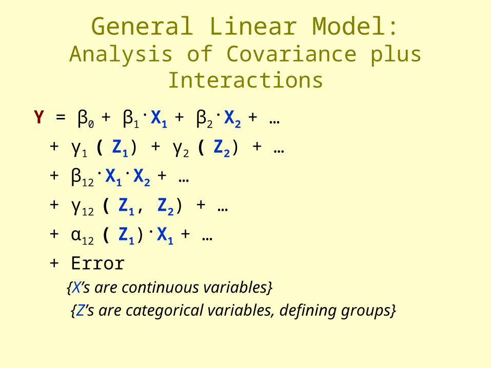
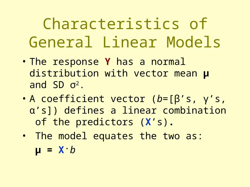
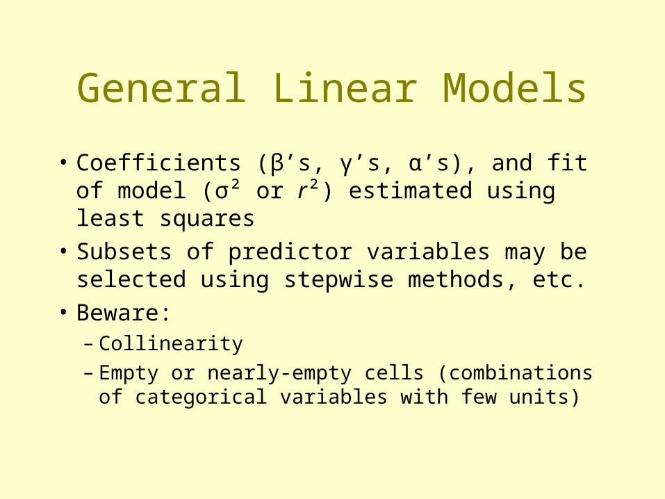
General Linear Models
bull Coefficients (βrsquos γrsquos αrsquos) and fit of model (σsup2 or rsup2) estimated using least squares
bull Subsets of predictor variables may be selected using stepwise methods etc
bull Bewarendash Collinearityndash Empty or nearly-empty cells (combinations of
categorical variables with few units)
General Linear Model
bull Datandash Movements of sperm whales (displacement per
12-hr) off Galapagos Islands with year clan and shit rate
bull Questionsndash Are movements of sperm whales affected by year
clan shit rate or combinations of them
General Linear Model
Potential X variablesYear (Categorical 1987 and 1989)Clan (Categorical lsquoPlus-onersquo and lsquoRegularrsquo)Shit-rate (Continuous Arcsine-Squareroot transform)YearClanYearShit-rateClanShit-rate
General Linear Model
X variables selected by stepwise selection (P-to-enter = 015 P-to-remove = 015)
Backward ForwardYear Year
Clan Clan
Shit-rate Shit-rate
YearClan YearClan
YearShit-rate YearShit-rate
ClanShit-rate ClanShit-rate
General Linear Model
bull BackwardY =c + Clan + YearClan
bull ForwardY =c + Shit-rateClan
1987 1989YEAR
0
10
20
30
40
50
60
12-h
r D
ispl
acem
ent (
km)
Reg+1
CL
01 02 03 04 05 06 07 08 09Shit rate (transformed)
0
10
20
30
40
50
60
12-h
r D
ispl
acem
ent (
km)
Reg+1
CL
General Linear Model
Why two ldquobest modelsrdquo
bull BackwardY =c + Clan + YearClan
bull ForwardY =c + Shit-rateClan
1987 1989YEAR
0
10
20
30
40
50
60
12-h
r D
ispl
acem
ent (
km)
Reg+1
CL
01 02 03 04 05 06 07 08 09Shit rate (transformed)
0
10
20
30
40
50
60
12-h
r D
ispl
acem
ent (
km)
Reg+1
CL
1987 1989
General Linear Model
Which is ldquobestrdquo
bull BackwardY =c + Clan + YearClan
bull ForwardY =c + Shit-rateClan
1987 1989YEAR
0
10
20
30
40
50
60
12-h
r D
ispl
acem
ent (
km)
Reg+1
CL
01 02 03 04 05 06 07 08 09Shit rate (transformed)
0
10
20
30
40
50
60
12-h
r D
ispl
acem
ent (
km)
Reg+1
CL
1987 1989
rsup2=02642 df
rsup2=03471 df
General Linear Models
bull The response Y has a normal distribution with vector mean μ and SD σ2
bull A coefficient vector (b=[βrsquos γrsquos αrsquos]) defines a linear combination of the predictors (Xrsquos)
bull The model equates the two as
μ = Xb
Generalized Linear Modelsbull The response Y has a distribution that may be
normal binomial Poisson gamma or inverse Gaussian with parameters including a mean micro
bull A coefficient vector (b=[βrsquos γrsquos αrsquos]) defines a linear combination of the predictors (Xrsquos)
bull A link function f defines the link between the two as
f(μ) = Xb
Generalized linear models
bull Examine assumptions using residuals
bull Examine fit using ldquodeviancerdquondash a generalization of the residual sum of squaresndash twice difference of log-likelihoods of model in
question and full modelndash fits of different models can be compared ndash Related to AIC
-1 0 1 20
05
1Logistic function
90 91 92 93 94 95 96 97 98 991000
10
20
30
40Binomial distribution
05 1 15 205
1
15
2Reciprocal function
0 1 2 3 4 5 6 7 8 9 100
10
20
30Poisson distribution
Generalized Linear Modelscan fit non-linear relationships using
lsquolink functionsrsquo and can consider non-normal errors
MATLAB glmdemo
Proportion of sexually-mature animals at different weights
2000 2500 3000 3500 4000 45000
01
02
03
04
05
06
07
08
09
1
Weight
Pro
port
ion
MATLAB glmdemo
Two problems with linear regression1) probabilities lt0 and gt1
2) clearly non-linear
2000 2500 3000 3500 4000 4500-02
0
02
04
06
08
1
12
Weight
Pro
port
ion
MATLAB glmdemo
Polynomial Regression better but also
1) probabilities lt0 and gt1
2) inflections are not real
2000 2500 3000 3500 4000 4500-02
0
02
04
06
08
1
12
Weight
Pro
port
ion
MATLAB glmdemo
Instead fit ldquologistic regressionrdquousing generalized linear model and
binomial distribution
MATLAB glmdemo
2000 2500 3000 3500 4000 45000
01
02
03
04
05
06
07
08
09
1
Weight
Pro
port
ion
sexu
ally
mat
ure
Y= 1(1+e β0+β1X)
2000 2500 3000 3500 4000 45000
01
02
03
04
05
06
07
08
09
1
Weight
Pro
port
ion
sexu
ally
mat
ure
Compare two generalized linear models
MATLAB glmdemo
Y= 1(1+e β0+β1X)
Y= 1(1+e β0+β1X +β2XX)
Difference in deviance =070 P=040
Examine assumptions using residuals
-1 -05 0 05 1
005
010
025
050
075
090
095
Data
Pro
babi
lity
Normal Probability Plot
MATLAB glmdemo
Making predictions
2400 2600 2800 3000 3200 3400 3600 3800 4000 42000
10
20
30
40
50
60
70
80
90
100
Weight
Pro
babi
lity
sexu
ally
mat
ure
MATLAB glmdemo
Non-linear models eg
Y = c + EXP(szlig0 + szlig1X) + E
Y = szlig0 + szlig1X[XgtXK] + Ebull More general than generalized linear
models
bull But harder to fitndash iterative processndash may not convergendash non-unique solutionndash harder to compare
SummaryMethods with One Dependent
Variable Simple Linear Regression One-way ANOVA
Multiple Linear Regression Multi-way ANOVA
Analysis of Covariance
General Linear Model
Generalized Linear Model
Non-Linear Model
IncreasingComplexity
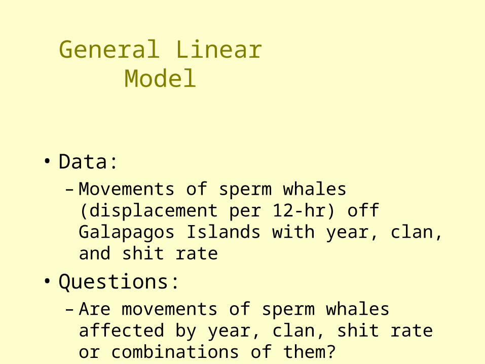
General Linear Model
bull Datandash Movements of sperm whales (displacement per
12-hr) off Galapagos Islands with year clan and shit rate
bull Questionsndash Are movements of sperm whales affected by year
clan shit rate or combinations of them
General Linear Model
Potential X variablesYear (Categorical 1987 and 1989)Clan (Categorical lsquoPlus-onersquo and lsquoRegularrsquo)Shit-rate (Continuous Arcsine-Squareroot transform)YearClanYearShit-rateClanShit-rate
General Linear Model
X variables selected by stepwise selection (P-to-enter = 015 P-to-remove = 015)
Backward ForwardYear Year
Clan Clan
Shit-rate Shit-rate
YearClan YearClan
YearShit-rate YearShit-rate
ClanShit-rate ClanShit-rate
General Linear Model
bull BackwardY =c + Clan + YearClan
bull ForwardY =c + Shit-rateClan
1987 1989YEAR
0
10
20
30
40
50
60
12-h
r D
ispl
acem
ent (
km)
Reg+1
CL
01 02 03 04 05 06 07 08 09Shit rate (transformed)
0
10
20
30
40
50
60
12-h
r D
ispl
acem
ent (
km)
Reg+1
CL
General Linear Model
Why two ldquobest modelsrdquo
bull BackwardY =c + Clan + YearClan
bull ForwardY =c + Shit-rateClan
1987 1989YEAR
0
10
20
30
40
50
60
12-h
r D
ispl
acem
ent (
km)
Reg+1
CL
01 02 03 04 05 06 07 08 09Shit rate (transformed)
0
10
20
30
40
50
60
12-h
r D
ispl
acem
ent (
km)
Reg+1
CL
1987 1989
General Linear Model
Which is ldquobestrdquo
bull BackwardY =c + Clan + YearClan
bull ForwardY =c + Shit-rateClan
1987 1989YEAR
0
10
20
30
40
50
60
12-h
r D
ispl
acem
ent (
km)
Reg+1
CL
01 02 03 04 05 06 07 08 09Shit rate (transformed)
0
10
20
30
40
50
60
12-h
r D
ispl
acem
ent (
km)
Reg+1
CL
1987 1989
rsup2=02642 df
rsup2=03471 df
General Linear Models
bull The response Y has a normal distribution with vector mean μ and SD σ2
bull A coefficient vector (b=[βrsquos γrsquos αrsquos]) defines a linear combination of the predictors (Xrsquos)
bull The model equates the two as
μ = Xb
Generalized Linear Modelsbull The response Y has a distribution that may be
normal binomial Poisson gamma or inverse Gaussian with parameters including a mean micro
bull A coefficient vector (b=[βrsquos γrsquos αrsquos]) defines a linear combination of the predictors (Xrsquos)
bull A link function f defines the link between the two as
f(μ) = Xb
Generalized linear models
bull Examine assumptions using residuals
bull Examine fit using ldquodeviancerdquondash a generalization of the residual sum of squaresndash twice difference of log-likelihoods of model in
question and full modelndash fits of different models can be compared ndash Related to AIC
-1 0 1 20
05
1Logistic function
90 91 92 93 94 95 96 97 98 991000
10
20
30
40Binomial distribution
05 1 15 205
1
15
2Reciprocal function
0 1 2 3 4 5 6 7 8 9 100
10
20
30Poisson distribution
Generalized Linear Modelscan fit non-linear relationships using
lsquolink functionsrsquo and can consider non-normal errors
MATLAB glmdemo
Proportion of sexually-mature animals at different weights
2000 2500 3000 3500 4000 45000
01
02
03
04
05
06
07
08
09
1
Weight
Pro
port
ion
MATLAB glmdemo
Two problems with linear regression1) probabilities lt0 and gt1
2) clearly non-linear
2000 2500 3000 3500 4000 4500-02
0
02
04
06
08
1
12
Weight
Pro
port
ion
MATLAB glmdemo
Polynomial Regression better but also
1) probabilities lt0 and gt1
2) inflections are not real
2000 2500 3000 3500 4000 4500-02
0
02
04
06
08
1
12
Weight
Pro
port
ion
MATLAB glmdemo
Instead fit ldquologistic regressionrdquousing generalized linear model and
binomial distribution
MATLAB glmdemo
2000 2500 3000 3500 4000 45000
01
02
03
04
05
06
07
08
09
1
Weight
Pro
port
ion
sexu
ally
mat
ure
Y= 1(1+e β0+β1X)
2000 2500 3000 3500 4000 45000
01
02
03
04
05
06
07
08
09
1
Weight
Pro
port
ion
sexu
ally
mat
ure
Compare two generalized linear models
MATLAB glmdemo
Y= 1(1+e β0+β1X)
Y= 1(1+e β0+β1X +β2XX)
Difference in deviance =070 P=040
Examine assumptions using residuals
-1 -05 0 05 1
005
010
025
050
075
090
095
Data
Pro
babi
lity
Normal Probability Plot
MATLAB glmdemo
Making predictions
2400 2600 2800 3000 3200 3400 3600 3800 4000 42000
10
20
30
40
50
60
70
80
90
100
Weight
Pro
babi
lity
sexu
ally
mat
ure
MATLAB glmdemo
Non-linear models eg
Y = c + EXP(szlig0 + szlig1X) + E
Y = szlig0 + szlig1X[XgtXK] + Ebull More general than generalized linear
models
bull But harder to fitndash iterative processndash may not convergendash non-unique solutionndash harder to compare
SummaryMethods with One Dependent
Variable Simple Linear Regression One-way ANOVA
Multiple Linear Regression Multi-way ANOVA
Analysis of Covariance
General Linear Model
Generalized Linear Model
Non-Linear Model
IncreasingComplexity
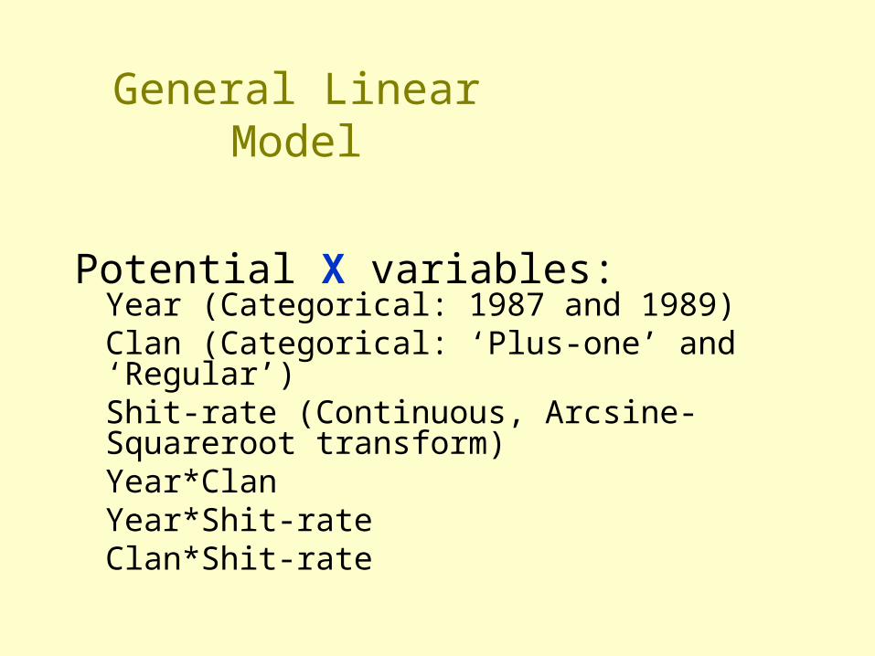
General Linear Model
Potential X variablesYear (Categorical 1987 and 1989)Clan (Categorical lsquoPlus-onersquo and lsquoRegularrsquo)Shit-rate (Continuous Arcsine-Squareroot transform)YearClanYearShit-rateClanShit-rate
General Linear Model
X variables selected by stepwise selection (P-to-enter = 015 P-to-remove = 015)
Backward ForwardYear Year
Clan Clan
Shit-rate Shit-rate
YearClan YearClan
YearShit-rate YearShit-rate
ClanShit-rate ClanShit-rate
General Linear Model
bull BackwardY =c + Clan + YearClan
bull ForwardY =c + Shit-rateClan
1987 1989YEAR
0
10
20
30
40
50
60
12-h
r D
ispl
acem
ent (
km)
Reg+1
CL
01 02 03 04 05 06 07 08 09Shit rate (transformed)
0
10
20
30
40
50
60
12-h
r D
ispl
acem
ent (
km)
Reg+1
CL
General Linear Model
Why two ldquobest modelsrdquo
bull BackwardY =c + Clan + YearClan
bull ForwardY =c + Shit-rateClan
1987 1989YEAR
0
10
20
30
40
50
60
12-h
r D
ispl
acem
ent (
km)
Reg+1
CL
01 02 03 04 05 06 07 08 09Shit rate (transformed)
0
10
20
30
40
50
60
12-h
r D
ispl
acem
ent (
km)
Reg+1
CL
1987 1989
General Linear Model
Which is ldquobestrdquo
bull BackwardY =c + Clan + YearClan
bull ForwardY =c + Shit-rateClan
1987 1989YEAR
0
10
20
30
40
50
60
12-h
r D
ispl
acem
ent (
km)
Reg+1
CL
01 02 03 04 05 06 07 08 09Shit rate (transformed)
0
10
20
30
40
50
60
12-h
r D
ispl
acem
ent (
km)
Reg+1
CL
1987 1989
rsup2=02642 df
rsup2=03471 df
General Linear Models
bull The response Y has a normal distribution with vector mean μ and SD σ2
bull A coefficient vector (b=[βrsquos γrsquos αrsquos]) defines a linear combination of the predictors (Xrsquos)
bull The model equates the two as
μ = Xb
Generalized Linear Modelsbull The response Y has a distribution that may be
normal binomial Poisson gamma or inverse Gaussian with parameters including a mean micro
bull A coefficient vector (b=[βrsquos γrsquos αrsquos]) defines a linear combination of the predictors (Xrsquos)
bull A link function f defines the link between the two as
f(μ) = Xb
Generalized linear models
bull Examine assumptions using residuals
bull Examine fit using ldquodeviancerdquondash a generalization of the residual sum of squaresndash twice difference of log-likelihoods of model in
question and full modelndash fits of different models can be compared ndash Related to AIC
-1 0 1 20
05
1Logistic function
90 91 92 93 94 95 96 97 98 991000
10
20
30
40Binomial distribution
05 1 15 205
1
15
2Reciprocal function
0 1 2 3 4 5 6 7 8 9 100
10
20
30Poisson distribution
Generalized Linear Modelscan fit non-linear relationships using
lsquolink functionsrsquo and can consider non-normal errors
MATLAB glmdemo
Proportion of sexually-mature animals at different weights
2000 2500 3000 3500 4000 45000
01
02
03
04
05
06
07
08
09
1
Weight
Pro
port
ion
MATLAB glmdemo
Two problems with linear regression1) probabilities lt0 and gt1
2) clearly non-linear
2000 2500 3000 3500 4000 4500-02
0
02
04
06
08
1
12
Weight
Pro
port
ion
MATLAB glmdemo
Polynomial Regression better but also
1) probabilities lt0 and gt1
2) inflections are not real
2000 2500 3000 3500 4000 4500-02
0
02
04
06
08
1
12
Weight
Pro
port
ion
MATLAB glmdemo
Instead fit ldquologistic regressionrdquousing generalized linear model and
binomial distribution
MATLAB glmdemo
2000 2500 3000 3500 4000 45000
01
02
03
04
05
06
07
08
09
1
Weight
Pro
port
ion
sexu
ally
mat
ure
Y= 1(1+e β0+β1X)
2000 2500 3000 3500 4000 45000
01
02
03
04
05
06
07
08
09
1
Weight
Pro
port
ion
sexu
ally
mat
ure
Compare two generalized linear models
MATLAB glmdemo
Y= 1(1+e β0+β1X)
Y= 1(1+e β0+β1X +β2XX)
Difference in deviance =070 P=040
Examine assumptions using residuals
-1 -05 0 05 1
005
010
025
050
075
090
095
Data
Pro
babi
lity
Normal Probability Plot
MATLAB glmdemo
Making predictions
2400 2600 2800 3000 3200 3400 3600 3800 4000 42000
10
20
30
40
50
60
70
80
90
100
Weight
Pro
babi
lity
sexu
ally
mat
ure
MATLAB glmdemo
Non-linear models eg
Y = c + EXP(szlig0 + szlig1X) + E
Y = szlig0 + szlig1X[XgtXK] + Ebull More general than generalized linear
models
bull But harder to fitndash iterative processndash may not convergendash non-unique solutionndash harder to compare
SummaryMethods with One Dependent
Variable Simple Linear Regression One-way ANOVA
Multiple Linear Regression Multi-way ANOVA
Analysis of Covariance
General Linear Model
Generalized Linear Model
Non-Linear Model
IncreasingComplexity
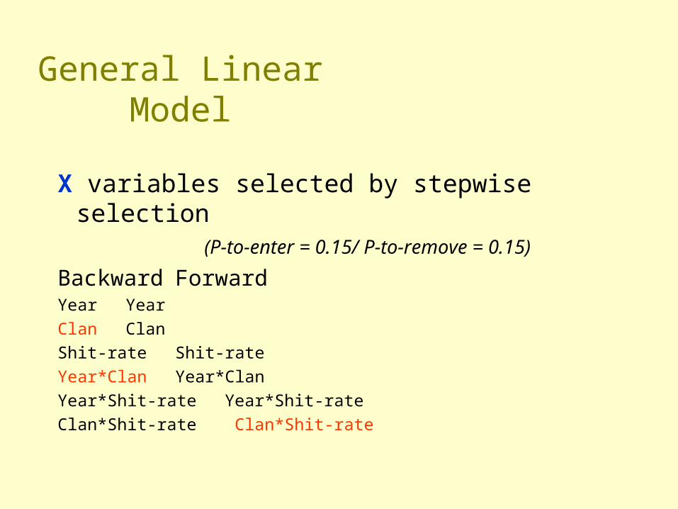
General Linear Model
X variables selected by stepwise selection (P-to-enter = 015 P-to-remove = 015)
Backward ForwardYear Year
Clan Clan
Shit-rate Shit-rate
YearClan YearClan
YearShit-rate YearShit-rate
ClanShit-rate ClanShit-rate
General Linear Model
bull BackwardY =c + Clan + YearClan
bull ForwardY =c + Shit-rateClan
1987 1989YEAR
0
10
20
30
40
50
60
12-h
r D
ispl
acem
ent (
km)
Reg+1
CL
01 02 03 04 05 06 07 08 09Shit rate (transformed)
0
10
20
30
40
50
60
12-h
r D
ispl
acem
ent (
km)
Reg+1
CL
General Linear Model
Why two ldquobest modelsrdquo
bull BackwardY =c + Clan + YearClan
bull ForwardY =c + Shit-rateClan
1987 1989YEAR
0
10
20
30
40
50
60
12-h
r D
ispl
acem
ent (
km)
Reg+1
CL
01 02 03 04 05 06 07 08 09Shit rate (transformed)
0
10
20
30
40
50
60
12-h
r D
ispl
acem
ent (
km)
Reg+1
CL
1987 1989
General Linear Model
Which is ldquobestrdquo
bull BackwardY =c + Clan + YearClan
bull ForwardY =c + Shit-rateClan
1987 1989YEAR
0
10
20
30
40
50
60
12-h
r D
ispl
acem
ent (
km)
Reg+1
CL
01 02 03 04 05 06 07 08 09Shit rate (transformed)
0
10
20
30
40
50
60
12-h
r D
ispl
acem
ent (
km)
Reg+1
CL
1987 1989
rsup2=02642 df
rsup2=03471 df
General Linear Models
bull The response Y has a normal distribution with vector mean μ and SD σ2
bull A coefficient vector (b=[βrsquos γrsquos αrsquos]) defines a linear combination of the predictors (Xrsquos)
bull The model equates the two as
μ = Xb
Generalized Linear Modelsbull The response Y has a distribution that may be
normal binomial Poisson gamma or inverse Gaussian with parameters including a mean micro
bull A coefficient vector (b=[βrsquos γrsquos αrsquos]) defines a linear combination of the predictors (Xrsquos)
bull A link function f defines the link between the two as
f(μ) = Xb
Generalized linear models
bull Examine assumptions using residuals
bull Examine fit using ldquodeviancerdquondash a generalization of the residual sum of squaresndash twice difference of log-likelihoods of model in
question and full modelndash fits of different models can be compared ndash Related to AIC
-1 0 1 20
05
1Logistic function
90 91 92 93 94 95 96 97 98 991000
10
20
30
40Binomial distribution
05 1 15 205
1
15
2Reciprocal function
0 1 2 3 4 5 6 7 8 9 100
10
20
30Poisson distribution
Generalized Linear Modelscan fit non-linear relationships using
lsquolink functionsrsquo and can consider non-normal errors
MATLAB glmdemo
Proportion of sexually-mature animals at different weights
2000 2500 3000 3500 4000 45000
01
02
03
04
05
06
07
08
09
1
Weight
Pro
port
ion
MATLAB glmdemo
Two problems with linear regression1) probabilities lt0 and gt1
2) clearly non-linear
2000 2500 3000 3500 4000 4500-02
0
02
04
06
08
1
12
Weight
Pro
port
ion
MATLAB glmdemo
Polynomial Regression better but also
1) probabilities lt0 and gt1
2) inflections are not real
2000 2500 3000 3500 4000 4500-02
0
02
04
06
08
1
12
Weight
Pro
port
ion
MATLAB glmdemo
Instead fit ldquologistic regressionrdquousing generalized linear model and
binomial distribution
MATLAB glmdemo
2000 2500 3000 3500 4000 45000
01
02
03
04
05
06
07
08
09
1
Weight
Pro
port
ion
sexu
ally
mat
ure
Y= 1(1+e β0+β1X)
2000 2500 3000 3500 4000 45000
01
02
03
04
05
06
07
08
09
1
Weight
Pro
port
ion
sexu
ally
mat
ure
Compare two generalized linear models
MATLAB glmdemo
Y= 1(1+e β0+β1X)
Y= 1(1+e β0+β1X +β2XX)
Difference in deviance =070 P=040
Examine assumptions using residuals
-1 -05 0 05 1
005
010
025
050
075
090
095
Data
Pro
babi
lity
Normal Probability Plot
MATLAB glmdemo
Making predictions
2400 2600 2800 3000 3200 3400 3600 3800 4000 42000
10
20
30
40
50
60
70
80
90
100
Weight
Pro
babi
lity
sexu
ally
mat
ure
MATLAB glmdemo
Non-linear models eg
Y = c + EXP(szlig0 + szlig1X) + E
Y = szlig0 + szlig1X[XgtXK] + Ebull More general than generalized linear
models
bull But harder to fitndash iterative processndash may not convergendash non-unique solutionndash harder to compare
SummaryMethods with One Dependent
Variable Simple Linear Regression One-way ANOVA
Multiple Linear Regression Multi-way ANOVA
Analysis of Covariance
General Linear Model
Generalized Linear Model
Non-Linear Model
IncreasingComplexity
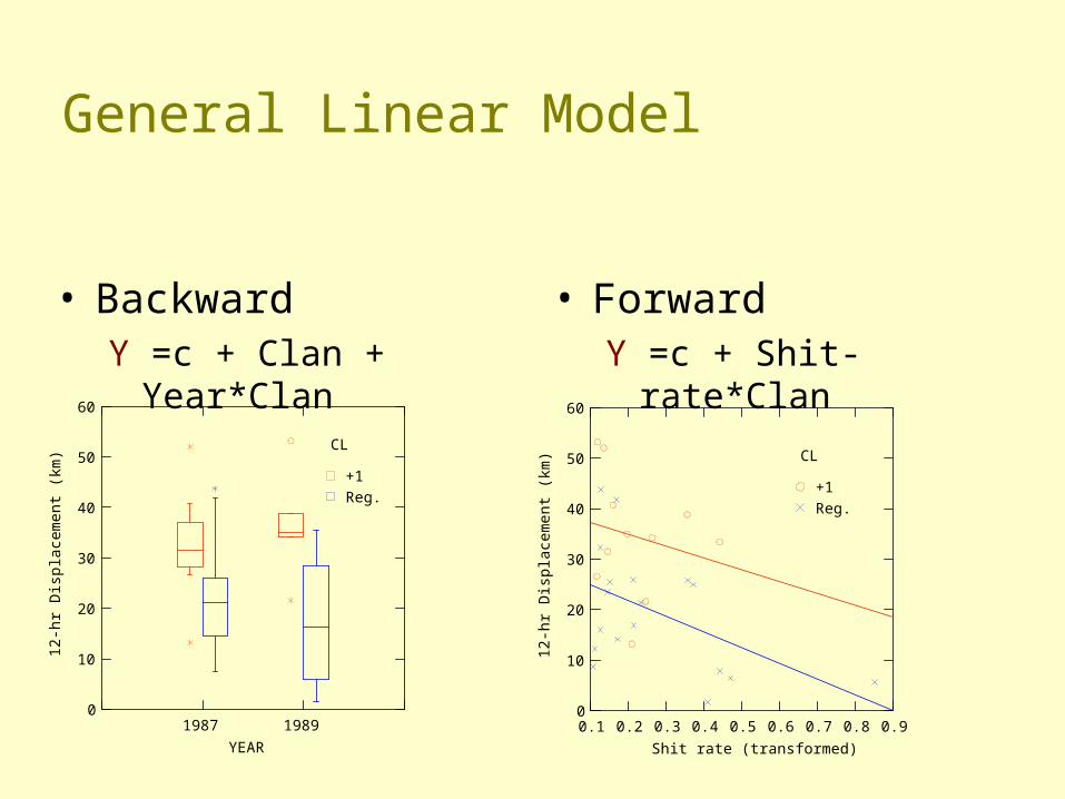
General Linear Model
bull BackwardY =c + Clan + YearClan
bull ForwardY =c + Shit-rateClan
1987 1989YEAR
0
10
20
30
40
50
60
12-h
r D
ispl
acem
ent (
km)
Reg+1
CL
01 02 03 04 05 06 07 08 09Shit rate (transformed)
0
10
20
30
40
50
60
12-h
r D
ispl
acem
ent (
km)
Reg+1
CL
General Linear Model
Why two ldquobest modelsrdquo
bull BackwardY =c + Clan + YearClan
bull ForwardY =c + Shit-rateClan
1987 1989YEAR
0
10
20
30
40
50
60
12-h
r D
ispl
acem
ent (
km)
Reg+1
CL
01 02 03 04 05 06 07 08 09Shit rate (transformed)
0
10
20
30
40
50
60
12-h
r D
ispl
acem
ent (
km)
Reg+1
CL
1987 1989
General Linear Model
Which is ldquobestrdquo
bull BackwardY =c + Clan + YearClan
bull ForwardY =c + Shit-rateClan
1987 1989YEAR
0
10
20
30
40
50
60
12-h
r D
ispl
acem
ent (
km)
Reg+1
CL
01 02 03 04 05 06 07 08 09Shit rate (transformed)
0
10
20
30
40
50
60
12-h
r D
ispl
acem
ent (
km)
Reg+1
CL
1987 1989
rsup2=02642 df
rsup2=03471 df
General Linear Models
bull The response Y has a normal distribution with vector mean μ and SD σ2
bull A coefficient vector (b=[βrsquos γrsquos αrsquos]) defines a linear combination of the predictors (Xrsquos)
bull The model equates the two as
μ = Xb
Generalized Linear Modelsbull The response Y has a distribution that may be
normal binomial Poisson gamma or inverse Gaussian with parameters including a mean micro
bull A coefficient vector (b=[βrsquos γrsquos αrsquos]) defines a linear combination of the predictors (Xrsquos)
bull A link function f defines the link between the two as
f(μ) = Xb
Generalized linear models
bull Examine assumptions using residuals
bull Examine fit using ldquodeviancerdquondash a generalization of the residual sum of squaresndash twice difference of log-likelihoods of model in
question and full modelndash fits of different models can be compared ndash Related to AIC
-1 0 1 20
05
1Logistic function
90 91 92 93 94 95 96 97 98 991000
10
20
30
40Binomial distribution
05 1 15 205
1
15
2Reciprocal function
0 1 2 3 4 5 6 7 8 9 100
10
20
30Poisson distribution
Generalized Linear Modelscan fit non-linear relationships using
lsquolink functionsrsquo and can consider non-normal errors
MATLAB glmdemo
Proportion of sexually-mature animals at different weights
2000 2500 3000 3500 4000 45000
01
02
03
04
05
06
07
08
09
1
Weight
Pro
port
ion
MATLAB glmdemo
Two problems with linear regression1) probabilities lt0 and gt1
2) clearly non-linear
2000 2500 3000 3500 4000 4500-02
0
02
04
06
08
1
12
Weight
Pro
port
ion
MATLAB glmdemo
Polynomial Regression better but also
1) probabilities lt0 and gt1
2) inflections are not real
2000 2500 3000 3500 4000 4500-02
0
02
04
06
08
1
12
Weight
Pro
port
ion
MATLAB glmdemo
Instead fit ldquologistic regressionrdquousing generalized linear model and
binomial distribution
MATLAB glmdemo
2000 2500 3000 3500 4000 45000
01
02
03
04
05
06
07
08
09
1
Weight
Pro
port
ion
sexu
ally
mat
ure
Y= 1(1+e β0+β1X)
2000 2500 3000 3500 4000 45000
01
02
03
04
05
06
07
08
09
1
Weight
Pro
port
ion
sexu
ally
mat
ure
Compare two generalized linear models
MATLAB glmdemo
Y= 1(1+e β0+β1X)
Y= 1(1+e β0+β1X +β2XX)
Difference in deviance =070 P=040
Examine assumptions using residuals
-1 -05 0 05 1
005
010
025
050
075
090
095
Data
Pro
babi
lity
Normal Probability Plot
MATLAB glmdemo
Making predictions
2400 2600 2800 3000 3200 3400 3600 3800 4000 42000
10
20
30
40
50
60
70
80
90
100
Weight
Pro
babi
lity
sexu
ally
mat
ure
MATLAB glmdemo
Non-linear models eg
Y = c + EXP(szlig0 + szlig1X) + E
Y = szlig0 + szlig1X[XgtXK] + Ebull More general than generalized linear
models
bull But harder to fitndash iterative processndash may not convergendash non-unique solutionndash harder to compare
SummaryMethods with One Dependent
Variable Simple Linear Regression One-way ANOVA
Multiple Linear Regression Multi-way ANOVA
Analysis of Covariance
General Linear Model
Generalized Linear Model
Non-Linear Model
IncreasingComplexity
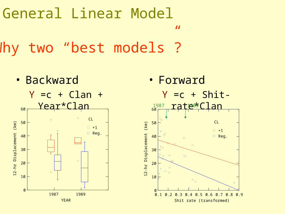
General Linear Model
Why two ldquobest modelsrdquo
bull BackwardY =c + Clan + YearClan
bull ForwardY =c + Shit-rateClan
1987 1989YEAR
0
10
20
30
40
50
60
12-h
r D
ispl
acem
ent (
km)
Reg+1
CL
01 02 03 04 05 06 07 08 09Shit rate (transformed)
0
10
20
30
40
50
60
12-h
r D
ispl
acem
ent (
km)
Reg+1
CL
1987 1989
General Linear Model
Which is ldquobestrdquo
bull BackwardY =c + Clan + YearClan
bull ForwardY =c + Shit-rateClan
1987 1989YEAR
0
10
20
30
40
50
60
12-h
r D
ispl
acem
ent (
km)
Reg+1
CL
01 02 03 04 05 06 07 08 09Shit rate (transformed)
0
10
20
30
40
50
60
12-h
r D
ispl
acem
ent (
km)
Reg+1
CL
1987 1989
rsup2=02642 df
rsup2=03471 df
General Linear Models
bull The response Y has a normal distribution with vector mean μ and SD σ2
bull A coefficient vector (b=[βrsquos γrsquos αrsquos]) defines a linear combination of the predictors (Xrsquos)
bull The model equates the two as
μ = Xb
Generalized Linear Modelsbull The response Y has a distribution that may be
normal binomial Poisson gamma or inverse Gaussian with parameters including a mean micro
bull A coefficient vector (b=[βrsquos γrsquos αrsquos]) defines a linear combination of the predictors (Xrsquos)
bull A link function f defines the link between the two as
f(μ) = Xb
Generalized linear models
bull Examine assumptions using residuals
bull Examine fit using ldquodeviancerdquondash a generalization of the residual sum of squaresndash twice difference of log-likelihoods of model in
question and full modelndash fits of different models can be compared ndash Related to AIC
-1 0 1 20
05
1Logistic function
90 91 92 93 94 95 96 97 98 991000
10
20
30
40Binomial distribution
05 1 15 205
1
15
2Reciprocal function
0 1 2 3 4 5 6 7 8 9 100
10
20
30Poisson distribution
Generalized Linear Modelscan fit non-linear relationships using
lsquolink functionsrsquo and can consider non-normal errors
MATLAB glmdemo
Proportion of sexually-mature animals at different weights
2000 2500 3000 3500 4000 45000
01
02
03
04
05
06
07
08
09
1
Weight
Pro
port
ion
MATLAB glmdemo
Two problems with linear regression1) probabilities lt0 and gt1
2) clearly non-linear
2000 2500 3000 3500 4000 4500-02
0
02
04
06
08
1
12
Weight
Pro
port
ion
MATLAB glmdemo
Polynomial Regression better but also
1) probabilities lt0 and gt1
2) inflections are not real
2000 2500 3000 3500 4000 4500-02
0
02
04
06
08
1
12
Weight
Pro
port
ion
MATLAB glmdemo
Instead fit ldquologistic regressionrdquousing generalized linear model and
binomial distribution
MATLAB glmdemo
2000 2500 3000 3500 4000 45000
01
02
03
04
05
06
07
08
09
1
Weight
Pro
port
ion
sexu
ally
mat
ure
Y= 1(1+e β0+β1X)
2000 2500 3000 3500 4000 45000
01
02
03
04
05
06
07
08
09
1
Weight
Pro
port
ion
sexu
ally
mat
ure
Compare two generalized linear models
MATLAB glmdemo
Y= 1(1+e β0+β1X)
Y= 1(1+e β0+β1X +β2XX)
Difference in deviance =070 P=040
Examine assumptions using residuals
-1 -05 0 05 1
005
010
025
050
075
090
095
Data
Pro
babi
lity
Normal Probability Plot
MATLAB glmdemo
Making predictions
2400 2600 2800 3000 3200 3400 3600 3800 4000 42000
10
20
30
40
50
60
70
80
90
100
Weight
Pro
babi
lity
sexu
ally
mat
ure
MATLAB glmdemo
Non-linear models eg
Y = c + EXP(szlig0 + szlig1X) + E
Y = szlig0 + szlig1X[XgtXK] + Ebull More general than generalized linear
models
bull But harder to fitndash iterative processndash may not convergendash non-unique solutionndash harder to compare
SummaryMethods with One Dependent
Variable Simple Linear Regression One-way ANOVA
Multiple Linear Regression Multi-way ANOVA
Analysis of Covariance
General Linear Model
Generalized Linear Model
Non-Linear Model
IncreasingComplexity
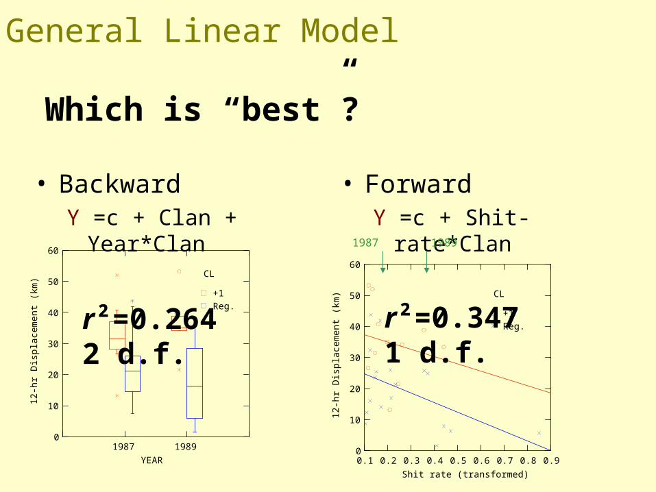
General Linear Model
Which is ldquobestrdquo
bull BackwardY =c + Clan + YearClan
bull ForwardY =c + Shit-rateClan
1987 1989YEAR
0
10
20
30
40
50
60
12-h
r D
ispl
acem
ent (
km)
Reg+1
CL
01 02 03 04 05 06 07 08 09Shit rate (transformed)
0
10
20
30
40
50
60
12-h
r D
ispl
acem
ent (
km)
Reg+1
CL
1987 1989
rsup2=02642 df
rsup2=03471 df
General Linear Models
bull The response Y has a normal distribution with vector mean μ and SD σ2
bull A coefficient vector (b=[βrsquos γrsquos αrsquos]) defines a linear combination of the predictors (Xrsquos)
bull The model equates the two as
μ = Xb
Generalized Linear Modelsbull The response Y has a distribution that may be
normal binomial Poisson gamma or inverse Gaussian with parameters including a mean micro
bull A coefficient vector (b=[βrsquos γrsquos αrsquos]) defines a linear combination of the predictors (Xrsquos)
bull A link function f defines the link between the two as
f(μ) = Xb
Generalized linear models
bull Examine assumptions using residuals
bull Examine fit using ldquodeviancerdquondash a generalization of the residual sum of squaresndash twice difference of log-likelihoods of model in
question and full modelndash fits of different models can be compared ndash Related to AIC
-1 0 1 20
05
1Logistic function
90 91 92 93 94 95 96 97 98 991000
10
20
30
40Binomial distribution
05 1 15 205
1
15
2Reciprocal function
0 1 2 3 4 5 6 7 8 9 100
10
20
30Poisson distribution
Generalized Linear Modelscan fit non-linear relationships using
lsquolink functionsrsquo and can consider non-normal errors
MATLAB glmdemo
Proportion of sexually-mature animals at different weights
2000 2500 3000 3500 4000 45000
01
02
03
04
05
06
07
08
09
1
Weight
Pro
port
ion
MATLAB glmdemo
Two problems with linear regression1) probabilities lt0 and gt1
2) clearly non-linear
2000 2500 3000 3500 4000 4500-02
0
02
04
06
08
1
12
Weight
Pro
port
ion
MATLAB glmdemo
Polynomial Regression better but also
1) probabilities lt0 and gt1
2) inflections are not real
2000 2500 3000 3500 4000 4500-02
0
02
04
06
08
1
12
Weight
Pro
port
ion
MATLAB glmdemo
Instead fit ldquologistic regressionrdquousing generalized linear model and
binomial distribution
MATLAB glmdemo
2000 2500 3000 3500 4000 45000
01
02
03
04
05
06
07
08
09
1
Weight
Pro
port
ion
sexu
ally
mat
ure
Y= 1(1+e β0+β1X)
2000 2500 3000 3500 4000 45000
01
02
03
04
05
06
07
08
09
1
Weight
Pro
port
ion
sexu
ally
mat
ure
Compare two generalized linear models
MATLAB glmdemo
Y= 1(1+e β0+β1X)
Y= 1(1+e β0+β1X +β2XX)
Difference in deviance =070 P=040
Examine assumptions using residuals
-1 -05 0 05 1
005
010
025
050
075
090
095
Data
Pro
babi
lity
Normal Probability Plot
MATLAB glmdemo
Making predictions
2400 2600 2800 3000 3200 3400 3600 3800 4000 42000
10
20
30
40
50
60
70
80
90
100
Weight
Pro
babi
lity
sexu
ally
mat
ure
MATLAB glmdemo
Non-linear models eg
Y = c + EXP(szlig0 + szlig1X) + E
Y = szlig0 + szlig1X[XgtXK] + Ebull More general than generalized linear
models
bull But harder to fitndash iterative processndash may not convergendash non-unique solutionndash harder to compare
SummaryMethods with One Dependent
Variable Simple Linear Regression One-way ANOVA
Multiple Linear Regression Multi-way ANOVA
Analysis of Covariance
General Linear Model
Generalized Linear Model
Non-Linear Model
IncreasingComplexity
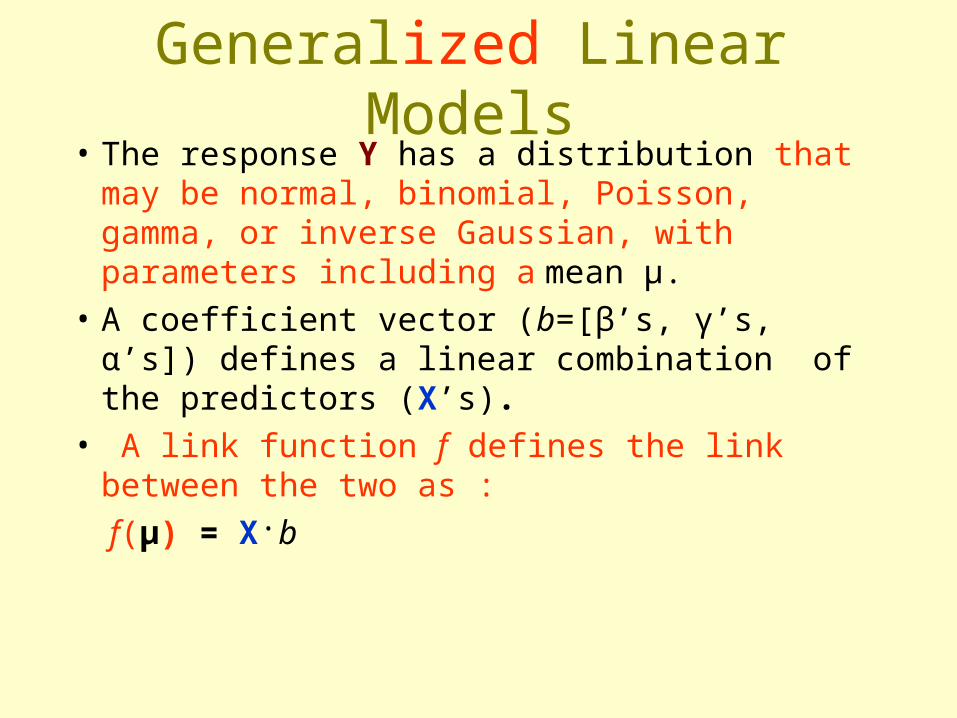
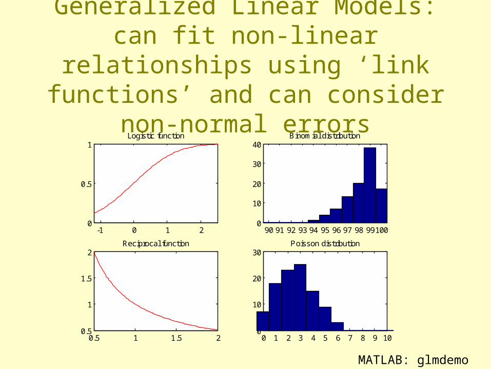
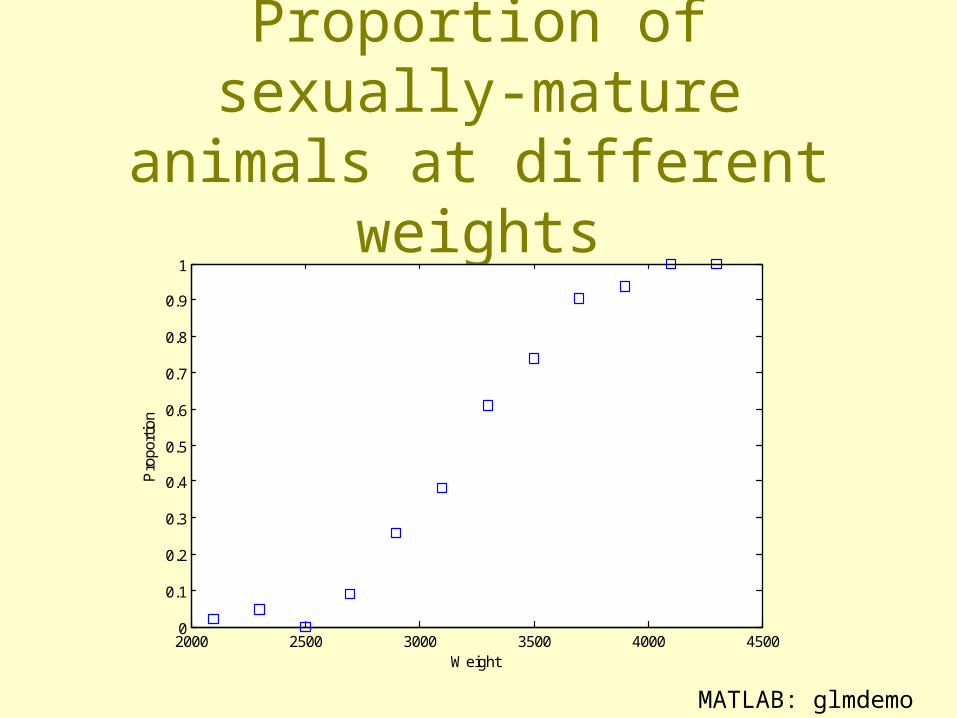
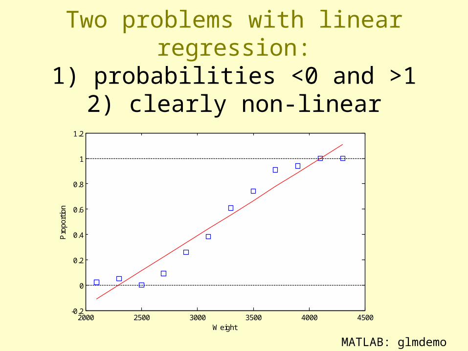
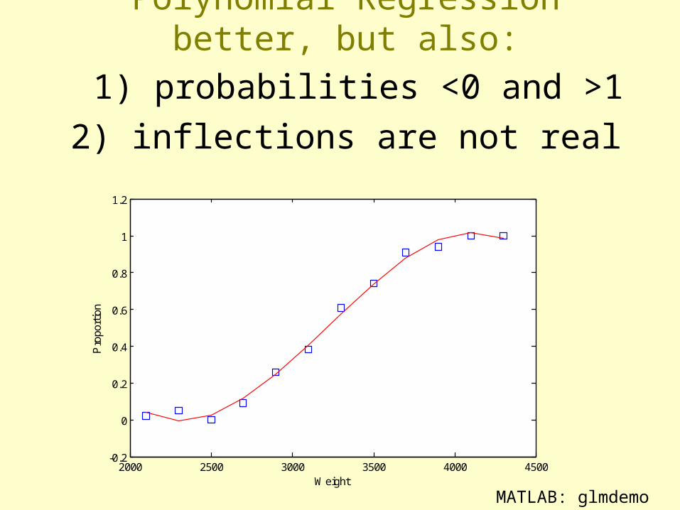
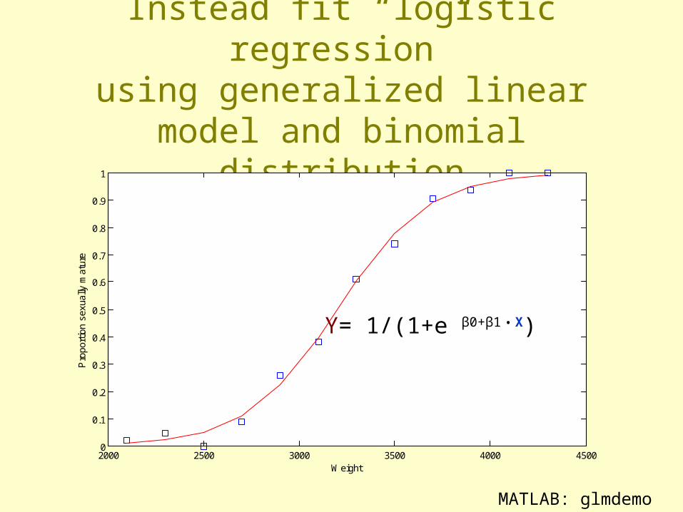
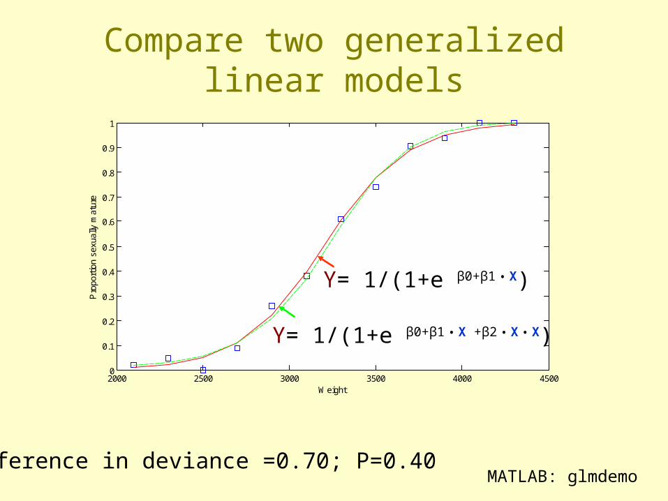
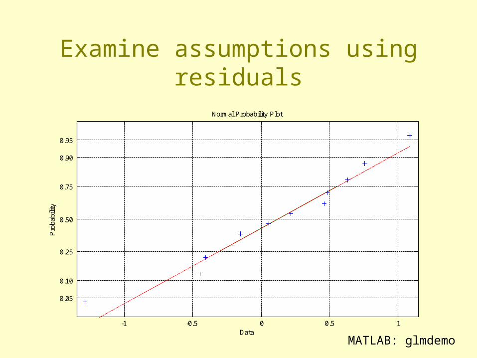
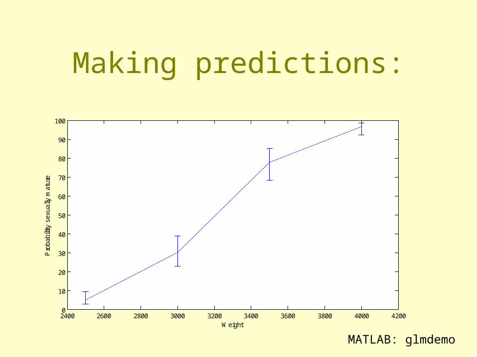
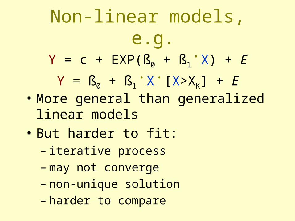
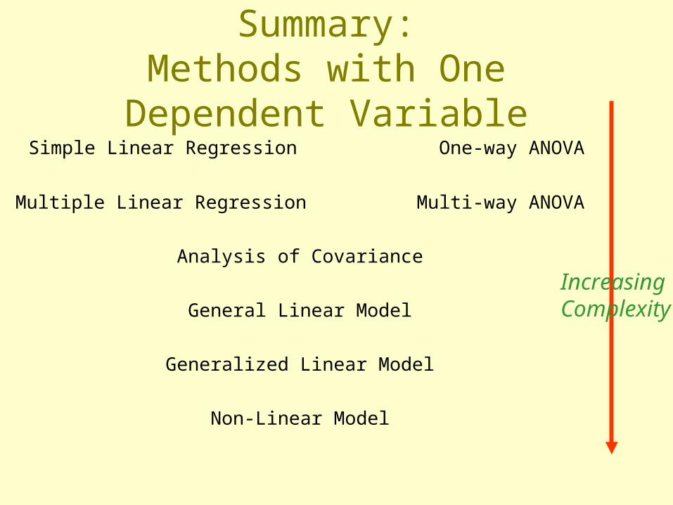
SummaryMethods with One Dependent
Variable Simple Linear Regression One-way ANOVA
Multiple Linear Regression Multi-way ANOVA
Analysis of Covariance
General Linear Model
Generalized Linear Model
Non-Linear Model
IncreasingComplexity