Generalized Low Rank Approximations of Matrices

Machine Learning, 61, 167–191, 20052005 Springer Science + Business Media, Inc. Manufactured in The Netherlands.

DOI: 10.1007/s10994-005-3561-6

Generalized Low Rank Approximations of MatricesJIEPING YE∗ [email protected] of Computer Science & Engineering,University of Minnesota-Twin Cities, Minneapolis,MN 55455, USA

Editor: Peter Flach

Published online: 12 August 2005

Abstract. The problem of computing low rank approximations of matrices is considered. The novel aspect of ourapproach is that the low rank approximations are on a collection of matrices. We formulate this as an optimizationproblem, which aims to minimize the reconstruction (approximation) error. To the best of our knowledge, theoptimization problem proposed in this paper does not admit a closed form solution. We thus derive an iterativealgorithm, namely GLRAM, which stands for the Generalized Low Rank Approximations of Matrices. GLRAMreduces the reconstruction error sequentially, and the resulting approximation is thus improved during successiveiterations. Experimental results show that the algorithm converges rapidly.

We have conducted extensive experiments on image data to evaluate the effectiveness of the proposed algorithmand compare the computed low rank approximations with those obtained from traditional Singular Value Decom-position (SVD) based methods. The comparison is based on the reconstruction error, misclassification error rate,and computation time. Results show that GLRAM is competitive with SVD for classification, while it has a muchlower computation cost. However, GLRAM results in a larger reconstruction error than SVD. To further reducethe reconstruction error, we study the combination of GLRAM and SVD, namely GLRAM + SVD, where SVD ispreceded by GLRAM. Results show that when using the same number of reduced dimensions, GLRAM + SVDachieves significant reduction of the reconstruction error as compared to GLRAM, while keeping the computationcost low.

Keywords: singular value decomposition, matrix approximation, reconstruction error, classification

1. Introduction

The problem of dimensionality reduction has recently received broad attention in areas suchas machine learning, computer vision, and information retrieval (Berry, Dumais, & O’Brie,1995; Castelli, Thomasian, & Li, 2003; Deerwester et al., 1990; Dhillon & Modha, 2001;Kleinberg & Tomkins, 1999; Srebro & Jaakkola, 2003). The goal of dimensionality reduc-tion is to obtain more compact representations of the data with limited loss of information.Traditional algorithms for dimensionality reduction are based on the so-called vector spacemodel. Under this model, each datum is modeled as a vector and the collection of data ismodeled as a single data matrix, where each column of the data matrix corresponds to adata point and each row corresponds to a feature dimension. The representation of data byvectors in Euclidean space allows one to compute the similarity between data points, based

∗Present address: Department of Computer Science & Engineering,Arizona State University, Tempe, AZ 85287-8809, USA .

168 J. YE

on the Euclidean distance or some other similarity metric. The similarity metrics on datapoints naturally lead to similarity-based indexing by representing queries as vectors andsearching for their nearest neighbors (Aggarwal, 2001; Castelli, Thomasian, & Li, 2003).

A well-known technique for dimensionality reduction is the low rank approximationby the Singular Value Decomposition (SVD), also called Latent Semantic Indexing (LSI)in information retrieval (Berry, Dumais, & O’Brie, 1995). An appealing property of thislow rank approximation is that it achieves the smallest reconstruction error among allapproximations with the same rank. Details can be found in Section 2. Some theoreticaljustification of the empirical success of LSI can be found in Papadimitriou et al. (1998),where it is shown that LSI works in the context of a simple probabilistic “Corpus-generating”model. However, applications of this technique to high-dimensional data, such as images andvideos, quickly run up against practical computational limits, mainly due to the expensiveSVD computation in both time and space for large matrices (Golub & Van Loan, 1996).

Several incremental algorithms have been proposed in the past (Brand, 2002; Gu &Eisenstat, 1993; Kanth et al., 1998) to deal with the high space complexity of SVD, wherethe data points are inserted incrementally to update the SVD. To the best of our knowledge,such algorithms come with no guarantees on the quality of the approximation produced.Random sampling can be applied to speed up the SVD computation. More details can befound in Achlioptas and McSherry (2001), Drineas et al. (1999) and Frieze, Kannan, &Vempala (1998).

1.1. Contributions

In this paper, we present a novel approach to alleviate the expensive SVD computation.The novelty lies in a new data representation model. Under this model, each datum isrepresented as a matrix, instead of a vector, and the collection of data is represented as acollection of matrices, instead of a single data matrix. We formulate the problem of lowrank approximations as a new optimization problem, which approximates a collection ofmatrices with matrices of lower rank. To the best of our knowledge, there is no closedform solution for the new optimization problem. We thus derive an iterative algorithm,namely GLRAM. Detailed mathematical justification for this iterative procedure is givenin Section 3.

Both GLRAM and SVD aim to minimize the reconstruction error. The essential differenceis that GLRAM applies a bilinear transformation on the data. Such a bilinear transformationis particularly appropriate for data in matrix form, and often leads to lower computation costin comparison to SVD. We apply GLRAM on image compression and retrieval, where eachimage is represented in its native matrix form. To evaluate the proposed algorithm, we haveconducted extensive experiments on five well-known image datasets: PIX, ORL, AR, PIE,and USPS, where USPS consists of images of handwritten digits and the other four are faceimage datasets. GLRAM is compared with SVD, as well as 2DPCA, a recently proposedalgorithm for dimension reduction. (Details on 2DPCA can be found in Section 4.)

Results show that when using the same number of reduced dimensions, GLRAM iscompetitive with SVD for classification, while it has a much lower computation cost.However, GLRAM results in a larger reconstruction error than SVD. The underlying

GENERALIZED LOW RANK APPROXIMATIONS OF MATRICES 169

reason may be that GLRAM is able to utilize the locality property (e.g., smoothness in animage) intrinsic in the data, which leads to good classification performance. In terms ofcompression ratio1, GLRAM outperforms SVD, especially when the number of data pointsis relatively small compared to the number of dimensions. For large and high-dimensionaldatasets, the lack of available space becomes a critical issue. In this case, compression ratiois an important factor in evaluating different dimensionality reduction algorithms.

To further reduce the reconstruction error of GLRAM, we study the combination ofGLRAM and SVD, namely GLRAM + SVD, which applies SVD after the intermediatedimensionality reduction stage using GLRAM. The essence of this composite algorithmis a further dimensionality reduction stage by SVD following GLRAM. Since SVD isapplied to a low-dimensional space transformed by GLRAM, the second stage by SVDcan be implemented efficiently. We apply this algorithm to image datasets and compareit with GLRAM and SVD. Results show that when using the same number of reduceddimensions, GLRAM + SVD achieves a significant reduction of the reconstruction error ascompared to GLRAM, while keeping the computation cost small. The reconstruction errorof GLRAM + SVD is close to that of SVD, especially when the intermediate dimensionin the GLRAM stage is large, while it has a smaller computation cost than SVD.

In summary, GLRAM can be applied as a pre-processing step for SVD. The pre-processing by GLRAM reduces significantly the computation cost of the SVD computation,while keeping the reconstruction error small (see Section 5.6).

1.2. Organization of the paper

The rest of this paper is organized as follows. We give a brief overview of low rank approx-imations of matrices in Section 2. The problem of generalized low rank approximations ofmatrices is studied in Section 3. Some related work is presented in Section 4. A performancestudy is provided in Section 5. Conclusions and directions for future work can be found inSection 6.

A preliminary version of this paper appears in the Proceedings of the Twenty-FirstInternational Conference on Machine Learning, Alberta, Canada, pp. 887–894, 2004. Thissubmission is substantially extended and contains: (1) additional datasets in Section 5.1,such as RAND and USPS; (2) new experiments in Sections 5.2–5.4; and (3) inclusion ofGLRAM + SVD in Section 5.6.

The major notations used throughout the rest of this paper are listed in Table 1.

2. Low rank approximations of matrices

Traditional methods in information retrieval and machine learning deal with data in vector-ized representation. A collection of data is then stored in a single matrix A ∈ R

N×n, whereeach column of A corresponds to a vector in the N-dimensional space. A major benefit ofthis vector space model is that the algebraic structure of the vector space can be exploited(Berry, Dumais, & O’Brie, 1995).

For high-dimensional data, one would like to simplify the data, so that traditional machinelearning and statistical techniques can be applied. However, crucial information intrinsic

170 J. YE

Table 1. Notations.

Notations Descriptions

Ai The i-th data point in matrix form

r Number of rows in Ai

c Number of columns in Ai

L Transformation on the left side

R Transformation on the right side

Mi Reduced representation of Ai

�1 Number of rows in Mi

�2 Number of columns in Mi

d Common value for �1 and �2

k Number of reduced dimensions by SVD

A Data matrix of size N by n

n Number of training data points

N Dimension of training data (N = rc)

in the data should not be removed under this simplification. A widely used method forthis purpose is to approximate the single data matrix, A, with a matrix of lower rank.Mathematically, the optimal rank-k approximation of a matrix A, under the Frobenius normcan be formulated as follows:

Find a matrix B ∈ RN×nwith rank(B) = k, such that

B = arg minrank(B)=k

‖A − B‖F ,

where the Frobenius norm, ‖M‖F , of a matrix M = (Mi j ) is given by ‖M‖F =√∑

i, j M2i j .

The matrix B can be readily obtained by computing the Singular Value Decomposition(SVD) of A, as stated in the following theorem (Golub & Van Loan, 1996).

Theorem 2.1. Let the Singular Value Decomposition of A ∈ RN×n be A = U DV T ,

where U and V are orthogonal, D = diag(σ1, . . . , σr , 0, . . . , 0), σ1 ≥ · · · ≥ σr > 0 and r= rank(A). Then for 1 ≤ k ≤ r,

∑ri=k+1 σ 2

i = min{‖A − B‖2F |rank(B) = k}. The minimum

is achieved with B = bestk(A), where bestk(A) = Uk diag(σ1, . . . , σk)V Tk , and Uk and Vk

are the matrices formed by the first k columns of U and V respectively.

For any approximation M of A, we call ‖A − M‖F the reconstruction error of the ap-proximation. By Theorem 2.1, B = Ukdiag(σ1, . . . , σk)V T

k has the smallest reconstructionerror among all the rank-k approximations of A.

Under this approximation, each column, ai ∈ RN , of A can be approximated as ai ≈ UkaL

i ,for some ai

L ∈ Rk. Since Uk has orthonormal columns, ||Uk ai

L − Uk ajL|| = ||ai

L − ajL||, i.e.,

the Euclidean distance between two vectors are preserved under the orthogonal projection.It follows that ||ai−aj|| ≈ ||Uk ai

L − Uk ajL|| = ||ai

L − ajL||. Hence the proximity of ai and aj,


in the original high-dimensional space, can be approximated by computing the proximityof their reduced representations ai

L and ajL. The speed-up on a single distance computation

using the reduced representations is N/k. This forms the basis for Latent Semantic Indexing(Berry, Dumais, & O’Brie, 1995; Deerwester et al., 1990), used widely in informationalretrieval.

Another potential application of the above rank-k approximation is for data compression.Since each ai is approximated by Uk ai

L, where Uk is common for every ai, we need to keepUk and {ai

L}ni=1 only for all the approximations. Since Uk ∈ R

N×k and aiL ∈ R

k, for i =1, . . . , n, it requires nk + Nk = (n + N)k scalars to store the reduced representations. Thestorage saved, or compression ratio, using the rank-k approximation is thus nN/(n + N)k,since the original data matrix A is of size N by n.

3. Generalized low rank approximations of matrices

In this section, we study the problem of generalized low rank approximations of matrices,which aims to approximate a collection of matrices with lower rank. A key differencebetween this generalized problem and the low rank approximation problem discussed inthe last section, is the data representation model applied.

Recall that the vector space model is applied for the traditional low rank approximations.The vector space model leads to a simple and closed form solution for low rank approxima-tions by computing the SVD of the data matrix. However, the SVD computation restrictsits applicability to matrices of small size. Instead, we apply a different data representationmodel, under which each datum is represented as a matrix and the collection of data isrepresented as a collection of matrices.

3.1. Problem formulation

Let Ai ∈ Rr×c, for i = 1, . . . , n, be the n data points in the training set, where r and

c denote the number of rows and columns respectively for each Ai. We aim to computetwo matrices L ∈ R

r×�1 and R ∈ Rc×�2 with orthonormal columns, and n matrices Mi ∈

R�1×�2 , for i = 1, . . . , n, such that LMi RT approximates Ai, for all i. Here, �1 and �2 are

two pre-specified parameters that are best set to the same value, based on the experimentalresults in Section 5. Mathematically, we can formulate this as the following minimizationproblem: Computing optimal L, R and {Mi}n

i=1, which solve

minL∈R

r×�1 : LT L=I�1R∈R

c×�2 : RT R=I�2Mi ∈R

�1×�2 : i=1,...,n

n∑i=1

||Ai − L Mi RT ||2F . (1)

The matrices L and R in the above approximations act as the two-sided linear trans-formations on the data in matrix form. Recall that in the case of traditional low rankapproximations, one-sided transformation is applied, which is Uk in our previous discus-sions. Note that the Mi’s are not required to be diagonal.

172 J. YE

The generalized low rank approximations above naturally lead to two basic applications.

– Data compression: The matrices L, R, and {Mi}ni=1 can be used to recover the original n

matrices {Ai}ni=1, assuming LMi RT approximates Ai, for each i. It requires r �1 + c �2 + n

�1 �2 scalars to store L, R, and {Mi}ni=1. Hence, the storage saved, or the compression

ratio using the approximations is nrc/(r�1 + c�2 + n�1�2).– Distance computation: A common similarity metric on matrices is the Frobenius norm.

The distance between Ai and Aj is ||Ai−Aj ||F. Using the approximations, we have||Ai−Aj ||F ≈ ||LMi RT − LMj RT ||F = ||Mi − Mj ||F, since both L and R have or-thonormal columns. The computation cost of computing ||Ai−Aj ||F (resp. ||Mi − Mj ||F)is O(rc) (resp. O(�1 �2)). Hence, the speed-up on a single distance computation using theapproximations is rc/(�1�2).

Note that as �1 and �2 decrease, the speed-up on the distance computation and the com-pression ratio increase. However, small values of �1 and �2 may lead to loss of informationintrinsic in the original data. We discuss this trade-off in Section 5.

The formulation in Eq. (1) is general, in the sense that �1 and �2 can be different, i.e., Mi

can have an arbitrary shape. We will study the effect of the shape of Mi on the performanceof the approximations in Section 5.2.

3.2. The main algorithm

In this section, we show how to solve the minimization problem in Eq. (1). The followingtheorem shows that the Mi’s are determined by the transformation matrices L and R, whichsignificantly simplifies the minimization problem in Eq. (1).

Theorem 3.1. Let L, R and {Mi}ni=1 be the optimal solution to the minimization problem

in Eq. (1). Then Mi = LT Ai R, for every i.

Proof: By the property of the trace of matrices,

n∑i=1

||Ai − L Mi RT ||2F =n∑

i=1

trace((Ai − L Mi RT )(Ai − L Mi RT )T )

=n∑

i=1

trace(

Ai ATi

) +n∑

i=1

trace(Mi MT

i

)

− 2n∑

i=1

trace(L Mi RT AT

i

), (2)

where the second term∑n

i=1 trace(Mi MiT ) results from the fact that both L and R have

orthonormal columns, and trace(AB) = trace(BA), for any two matrices.


Since the first term on the right hand side of Eq. (2) is a constant, the minimization inEq. (1) is equivalent to minimizing

n∑i=1

trace(Mi MT

i

) − 2n∑

i=1

trace(L Mi RT AT

i

). (3)

It is easy to check that the minimum of (3) is achieved, only if Mi = LT Ai R, for every i.This completes the proof of the theorem. �

Theorem 3.1 implies that Mi is uniquely determined by L and R with Mi = LT Ai R, forall i. Hence the key step for the minimization in Eq. (1) is the computation of the commontransformations L and R. A key property of the optimal transformations L and R is statedin the following theorem:


in Eq. (1). Then L and R solve the following optimization problem:

maxL∈R

r×�1 : LT L=I�1R∈R

c×�2 : RT R=I�2

n∑i=1

||LT Ai R||2F . (4)

Proof: From Theorem 3.1, Mi = LT Ai R, for every i. Substituting this into∑n

i=1 ||Ai −LMi RT ||F2, we obtain

n∑i=1

||Ai − L Mi RT ||2F =n∑

i=1

||Ai ||2F −n∑

i=1

||LT Ai R||2F . (5)

Hence the minimization in Eq. (1) is equivalent to the maximization of

n∑i=1

||LT Ai R||2F ,

which completes the proof of the theorem. �

To the best of our knowledge, there is no closed form solution for the maximization prob-lem in Eq. (4). A key observation, which leads to an iterative algorithm for the computationof L and R, is stated in the following theorem:


in Eq. (1). Then(1) For a given R, L consists of the �1 eigenvectors of the matrix

ML =n∑

i=1

Ai R RT ATi

174 J. YE

corresponding to the largest �1 eigenvalues.(2) For a given L, R consists of the �2 eigenvectors of the matrix

MR =n∑

i=1

ATi L LT Ai

corresponding to the largest �2 eigenvalues.

Proof: By Theorem 3.2, L and R maximize

n∑i=1

||LT Ai R||2F ,

which can be rewritten as

n∑i=1

trace(LT Ai R RT AT

i L) = trace

(LT

n∑i=1

(Ai R RT AT

i

)L

)

= trace(LT ML L), (6)

where ML = ∑ni=1 Ai RRT Ai

T . Hence, for a given R, the maximum of

n∑i=1

||LT Ai R||2F = trace(LT ML L

)

is achieved, only if L ∈ Rr× �1 consists of the �1 eigenvectors of the matrix ML corresponding

to the largest �1 eigenvalues. The maximization of trace(LT ML L) can be considered as aspecial case of the more general optimization problem in Edelman, Arias and Smith (1998).

Similarly, by the property of the trace of matrices,

n∑i=1

||LT Ai R||2F

can also be rewritten as

n∑i=1

trace(RT AT

i L LT Ai R) = trace

(RT

n∑i=1

(AT

i L LT Ai)R

)

= trace(RT MR R), (7)

where MR = ∑ni=1 Ai

T LLT Ai . Hence, for a given L, the maximum of

n∑i=1

||LT Ai R||2F = trace(RT MR R)


is achieved, only if R ∈ Rc×�2 consists of the �2 eigenvectors of the matrix MR corresponding

to the largest �2 eigenvalues. This completes the proof of the theorem. �

Theorem 3.3 results in an iterative procedure for computing L and R as follows: for a givenL, we can compute R by computing the eigenvectors of the matrix MR; with the computedR, we can then update L by computing the eigenvectors of the matrix ML. The procedurecan be repeated until convergence. The pseudo-code of the above iterative procedure isgiven in Algorithm GLRAM below.

Theoretically, the solution to GLRAM is only locally optimal. The solution depends onthe choice of the initial L0 for L. We did extensive experiments (see Section 5.3) usingdifferent choices of the initial L0 and found out that, for image datasets, GLRAM alwaysconverges to the same solution, regardless of the choice of the initial L0.

Theorem 3.3 implies that the matrix updates in Lines 5 and 8 of GLRAM do not decreasethe value of

∑ni=1 ||LT Ai R ||F2, since the computed R and L are locally optimal. Hence by

Theorem 3.2, the value of∑n

i=1 ||Ai − LMi RT ||F2, or

RMSRE ≡√√√√1

n

n∑i=1

||Ai − L Mi RT ||2F (8)

176 J. YE

does not increase. Here RMSRE stands for the Root Mean Square Reconstruction Error.The convergence of GLRAM follows, since RMSRE is bounded from below by 0, as statedin the following Theorem:

Theorem 3.4. The GLRAM Algorithm monotonically non-increases the RMSRE value asdefined in Eq. (8), hence it converges in the limit.

Thus we use the relative reduction of the RMSRE value to check the convergence.Specifically, let RMSRE(i) be the RMSRE value at the i-th iteration of the GLRAMalgorithm, then the convergence of the algorithm is determined by checking whether thefollowing inequality holds:

RMSRE(i − 1) − RMSRE(i)

RMSRE(i − 1)< η,

for some small threshold η > 0. In our experiments, we choose η = 10−6. Results inSection 5 show that the algorithm converges within two to three iterations.

Note that the transformation matrices L and R in GLRAM may not converge, even whenthe RMSRE value converges. To see why this is the case, consider two pairs of solutions(L, R) and (LP, RQ), for some orthogonal matrices P ∈ R

�1×�1 and Q ∈ R�2×�2 . Since

RMSRE ≡√√√√1

n

n∑i=1

||Ai − L Mi RT ||2F =√√√√1

n

n∑i=1

||Ai − L LT Ai R RT ||2F ,

it is easy to verify that both (L, R) and (LP, RQ) result in the same RMSRE value.Thus, the solution to GLRAM is invariant under arbitrary orthogonal transformations. Twotransformations L and L can be compared by computing the largest principal angle ((Bjork& Golub, 1973; Golub & Van Loan, 1996) between the column spaces of L and L . If theangle is zero, L is essentially equivalent to L up to an orthogonal transformation.

3.3. Time and space complexities

The most expensive steps in GLRAM are the formation of the matrices MR and ML in Lines3 and 6, and the formation of Mj in Lines 13–15.

It takes O(�1 c (r + c) n) time for computing MR and O(�2 r (r + c) n) time for computingML. The computation time of Mj = (LT (Aj R)) using the given order is O(rc�2 + r�2�1) =O(r�2 (c + �1)). Assume the number of iterations in the while loop (from Line 2 to Line10) is I. The total time complexity of GLRAM is O(I(r + c)2 max (�1, �2) n).

It is easy to verify that the space complexity of GLRAM is O(rc) = O(N). The key to thelow space complexity is that the formation of the matrices MR and ML can be proceeded byreading the matrices {Ai}n

i=1 incrementally.Note that GLRAM involves eigenvalue problems of size r2 or c2, as compared to size

rcn (= Nn) in SVD. This is the key reason why GLRAM has much lower costs in time andspace than SVD.


4. Related work

Wavelet transform is a commonly used scheme for image compression (Averbuch, Lazar,& Israeli, 1996). Similar to the GLRAM algorithm in this paper, wavelets can be appliedto images in matrix representation. A subtle but important difference between waveletcompression and GLRAM compression is that the former mainly aims to compress andreconstruct a single image with small cost of basis representations, which is extremelyimportant for image transmission in computer networks, whereas GLRAM compressionaims to compress a set of images by making use of the correlation information betweenimages.

A collection of images can also be considered as a 3rd-order tensor, or three-dimensionalarray. Decomposition of higher-order tensors has been studied in Kolda (2001), Shashuaand Levin (2001), Vasilescu and Terzopoulos (2002), and Zhang and Golub (2001). Ourapproach differs in that we keep explicit the 2D nature of images.

The work that is most closely related to the current one is the two-dimensional PrincipalComponent Analysis (2DPCA) algorithm recently proposed in Yang et al. (2004). LikeGLRAM, 2DPCA works with data in matrix form. The key difference is that 2DPCAapplies linear transformation on the right side of the data, while GLRAM applies two-sidedlinear transformation. 2DPCA can be formulated as a trace optimization problem, fromwhich a closed form solution is obtained. However, a disadvantage of 2DPCA, as alsomentioned in Yang et al. (2004), is that the number of reduced dimensions of 2DPCA canbe quite large. More details are given below.

2DPCA computes a linear transformation X ∈ Rc×� with � < c, such that each image Ai

∈ Rr×c is transformed (projected) to Yi = Ai X ∈ R

r×�. The variance of the n projections{Yi}n

i=1 can be computed as

1

n − 1

n∑i=1

||Yi − Y ||2F = 1

n − 1

n∑i=1

X T (Ai − A)T (Ai − A)X,

where Y = 1n

∑ni=1 Yi = AX is the mean and A = 1

n

∑ni=1 Ai .

The optimal transformation X in 2DPCA is computed such that the variance of the n datapoints in the transformed space is maximized. Specifically, the optimal transformation Xcan be computed by solving the following maximization problem:

X = arg maxX T X=I�

(1

n − 1

n∑i=1

X T (Ai − A)T (Ai − A)X

). (9)

The optimal X can be obtained by computing the � eigenvectors of the matrix 1n−1

∑ni=1(Ai −

A)T (Ai − A) corresponding to the largest � eigenvalues.It requires c� + nr� scalars to store X ∈ R

c×� and {Yi}ni=1 ∈ R

r×�. Hence, the compressionratio by 2DPCA is nrc/(c� + nr�) ≈ c/�.

Table 2 lists the time and space complexities of SVD, 2DPCA, and GLRAM. It is clearthat GLRAM and 2DPCA have much smaller costs in time and space than SVD.

178 J. YE

Table 2. Comparison of SVD, 2DPCA, and GLRAM: n is the number of data points in the training dataset andN = r × c is the dimension of the data.

Methods Time Space

SVD O(nN min (n, N)) O(nN)

2DPCA O(nc2r) O(N)

GLRAM O(I(r+c)2 max (�1, �2) n) O(N)

5. Experimental evaluations

In this section, we experimentally evaluate the GLRAM algorithm. All of our ex-periments are performed on a P4 2.785 GHz Linux machine with 1GB memory.A MATLAB version of the GLRAM algorithm can be accessed at http://www-users.cs.umn.edu/∼jieping/GLRAM/}.

We present in Section 5.1 one synthetic dataset and five real-world image datasetsused for our evaluation. The effect of the ratio of �1 to �2 on reconstruction error isdiscussed in Section 5.2. Results show that, for the datasets considered in the paper,choosing �1/�2 ≈ 1 achieves good performance. We thus set both �1 and �2 equal to acommon value d in the following experiments. The sensitivity of GLRAM to the choice ofthe initial L0 for L is studied in Section 5.3. In Sections 5.4–5.5, a detailed comparative studybetween the proposed algorithm and SVD is provided, where the comparison is made onthe reconstruction error (measured by RMSRE), classification, and quality of compressedimages. The results with 2DPCA (Yang et al., 2004) are also included. The effectivenessof SVD critically depends on the reduced dimension k. For all the experiments, k is chosenso that both SVD and GLRAM have the same number of reduced dimensions. Finally, westudy the GLRAM + SVD algorithm in Section 5.6.

For all the experiments, we use the K-Nearest-Neighbors (K-NN) method with K = 1based on the Euclidean distance for classification (Duda, Hart, & Stork, 2000; Fukunaga,1990). We use 10-fold cross-validation for estimating the misclassification error rate. In10-fold cross-validation, we divide the data into ten subsets of approximately equal size.Then we do the training and testing ten times, each time leaving out one of the subsetsfor training, and using only the omitted subset for testing. The misclassification error ratereported is the average from the ten runs.

5.1. Datasets

We use the following six datasets (one synthetic dataset and five real-world image datasets)in our experiments:

– RAND is a synthetic dataset, consisting of 500 data points of size 100 × 100. All theentries are randomly generated between 0 and 255 (the same range as the four face imagedatasets).

– PIX2 contains 300 face images of 30 persons. The size of PIX images is 512 × 512. Wesubsample the images down to a size of 100 × 100 = 10000.


– ORL3 is a well-known dataset for face recognition (Samaria & Harter, 1994). It containsthe face images of 40 persons, for a total of 400 images. The image size is 92 × 112.The face images are perfectly centred. The major challenge posed by this dataset is thevariation of the face pose. We use the whole image as an instance (i.e., the dimension ofan instance is 92 × 112 = 10304).

– AR4 is a large face image dataset (Martinez & Benavente, 1998). The instance of eachface may contain large areas of occlusion, due to the presence of sun glasses and scarves.The existence of occlusion dramatically increases the within-class variances of AR faceimage data. We use a subset of AR. This subset contains 1638 face images of 126 persons.Its image size is 768 × 576. We first crop the image from row 100 to 500, and column200 to 550, and then subsample the cropped images down to a size of 101 × 88 = 8888.

– PIE5 is a subset of the CMU–PIE face image dataset (Sim et al., 2004). PIE contains 6615face instances of 63 persons. More specifically, each person has 21× 5 = 105 instancestaken under 21 different lighting conditions and 5 different poses. The image size of PIEis 640 × 480. We pre-process each image using a similar technique as above. The finaldimension of each instance is 32 × 24 = 768.

– USPS6 is an image dataset consisting of 9298 handwritten digits of “0” through “9”. Weuse a subset of USPS. This subset contains 300 images for each digit, for a total of 3000images. The image size is 16 × 16 = 256.

The statistics of all datasets are summarized in Table 3.

5.2. Effect of the ratio of �1 to �2 on reconstruction error

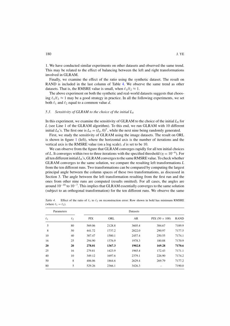
In this experiment, we study the effect of the ratio of �1 to �2 on reconstruction error,where �1 and �2 are the row and column dimensions of the reduced representation Mi inGLRAM. To this end, we run GLRAM with different combinations of �1 and �2 with aconstant product �1 · �2 = 400. The results on PIX, ORL, and AR are shown in Table 4. Itis clear from the table that the RMSRE value is small, when �1/�2 ≈ 1, and the minimumis achieved when �1/�2 = 1 in all cases.

To examine whether this is related to the fact that for images, the number of rows (r)and the number of columns (c) are comparable, we subsample the images in PIX down to asize of 50 × 100 = 5000. The result on this dataset is included in Table 4. Interestingly, weobserve the same trend in this dataset. That is, the RMSRE value is small, when �1/�2 ≈Table 3. Statistics of our test datasets.

Dataset Size (n) Dimension (r × c) Number of classes

RAND 500 100 × 100 = 10000 –

PIX 300 100 × 100 = 10000 30

ORL 400 92 × 112 = 10304 40

AR 1638 101 × 88 = 8888 126

PIE 6615 32 × 24 = 768 63

USPS 3000 16 × 16 = 256 10

180 J. YE

1. We have conducted similar experiments on other datasets and observed the same trend.This may be related to the effect of balancing between the left and right transformationsinvolved in GLRAM.

Finally, we examine the effect of the ratio using the synthetic dataset. The result onRAND is included in the last column of Table 4. We observe the same trend as otherdatasets. That is, the RMSRE value is small, when �1/�2 ≈ 1.

The above experiment on both the synthetic and real-world datasets suggests that choos-ing �1/�2 ≈ 1 may be a good strategy in practice. In all the following experiments, we setboth �1 and �2 equal to a common value d.

5.3. Sensitivity of GLRAM to the choice of the initial L0

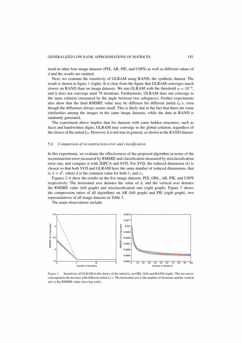
In this experiment, we examine the sensitivity of GLRAM to the choice of the initial L0 forL (see Line 1 of the GLRAM algorithm). To this end, we run GLRAM with 10 differentinitial L0’s. The first one is L0 = (Id, 0)T , while the next nine being randomly generated.

First, we study the sensitivity of GLRAM using the image datasets. The result on ORLis shown in figure 1 (left), where the horizontal axis is the number of iterations and thevertical axis is the RMSRE value (on a log scale). d is set to be 10.

We can observe from the figure that GLRAM converges rapidly for all ten initial choicesof L. It converges within two to three iterations with the specified threshold (η = 10−6). Forall ten different initial L0’s, GLRAM converges to the same RMSRE value. To check whetherGLRAM converges to the same solution, we compare the resulting left transformations Lfrom the ten different runs. Two transformations can be compared by computing the largestprincipal angle between the column spaces of these two transformations, as discussed inSection 3. The angle between the left transformation resulting from the first run and theones from other nine runs are computed (results omitted). For all cases, the angles arearound 10−10 to 10−7. This implies that GLRAM essentially converges to the same solution(subject to an orthogonal transformation) for the ten different runs. We observe the same

Table 4. Effect of the ratio of �1 to �2 on reconstruction error: Row shown in bold has minimum RMSRE(where �1 = �2).

Parameters Datasets

�1 �2 PIX ORL AR PIX (50 × 100) RAND

5 80 569.06 2128.8 3605.4 384.67 7189.9

8 50 441.72 1737.2 2822.0 290.97 7177.5

10 40 387.47 1580.1 2457.4 250.55 7174.1

16 25 294.90 1376.9 1978.3 180.88 7170.9

20 20 278.01 1367.3 1902.8 169.28 7170.6

25 16 279.81 1423.9 1965.4 172.43 7171.1

40 10 349.12 1697.6 2379.1 226.90 7174.2

50 8 406.06 1864.6 2629.4 269.79 7177.2

80 5 529.26 2366.1 3426.3 – 7190.0


trend in other four image datasets (PIX, AR, PIE, and USPS) as well as different values ofd and the results are omitted.

Next, we examine the sensitivity of GLRAM using RAND, the synthetic dataset. Theresult is shown in figure 1 (right). It is clear from the figure that GLRAM converges muchslower on RAND than on image datasets. We run GLRAM with the threshold η = 10−6,and it does not converge until 78 iterations. Furthermore, GLRAM does not converge tothe same solution (measured by the angle between two subspaces). Further experimentsalso show that the final RMSRE value may be different for different initial L0’s, eventhough the difference always seems small. This is likely due to the fact that there are somesimilarities among the images in the same image datasets, while the data in RAND israndomly generated.

The experiment above implies that for datasets with some hidden structures, such asfaces and handwritten digits, GLRAM may converge to the global solution, regardless ofthe choice of the initial L0. However, it is not true in general, as shown in the RAND dataset.

5.4. Comparison of reconstruction error and classification

In this experiment, we evaluate the effectiveness of the proposed algorithm in terms of thereconstruction error measured by RMSRE and classification measured by misclassificationerror rate, and compare it with 2DPCA and SVD. For SVD, the reduced dimension (k) ischosen so that both SVD and GLRAM have the same number of reduced dimensions, thatis, k = d2, where d is the common value for both �1 and �2.

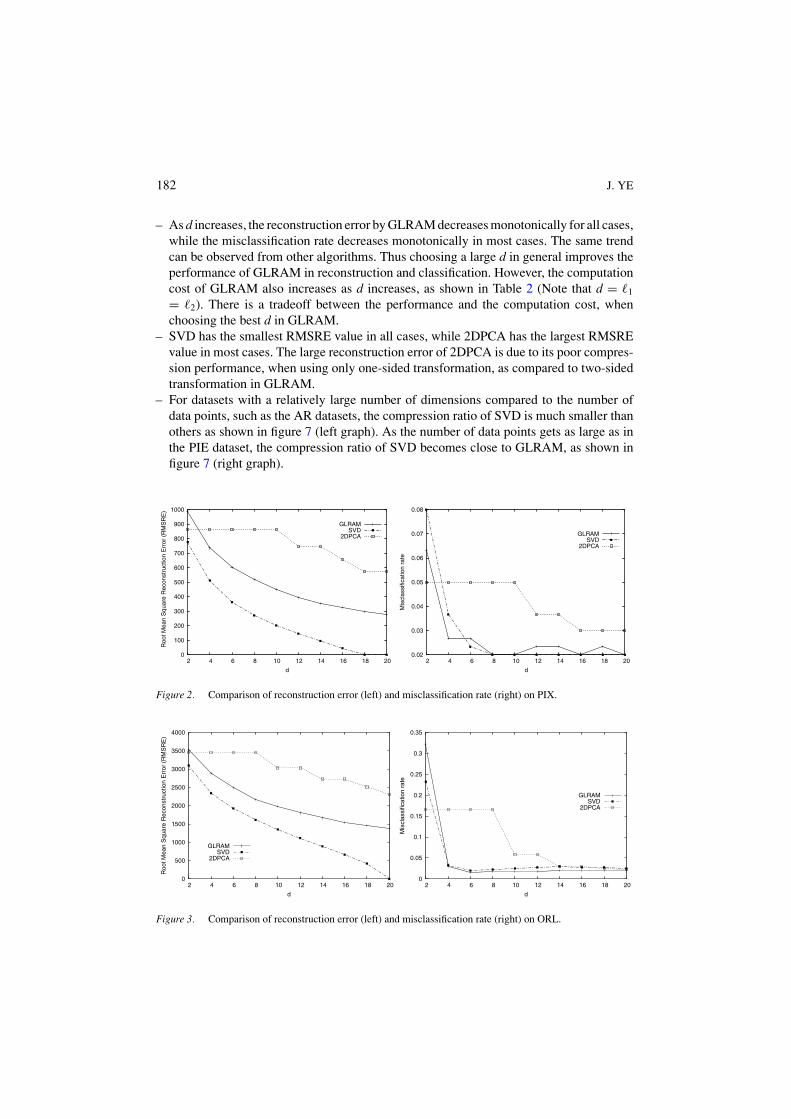
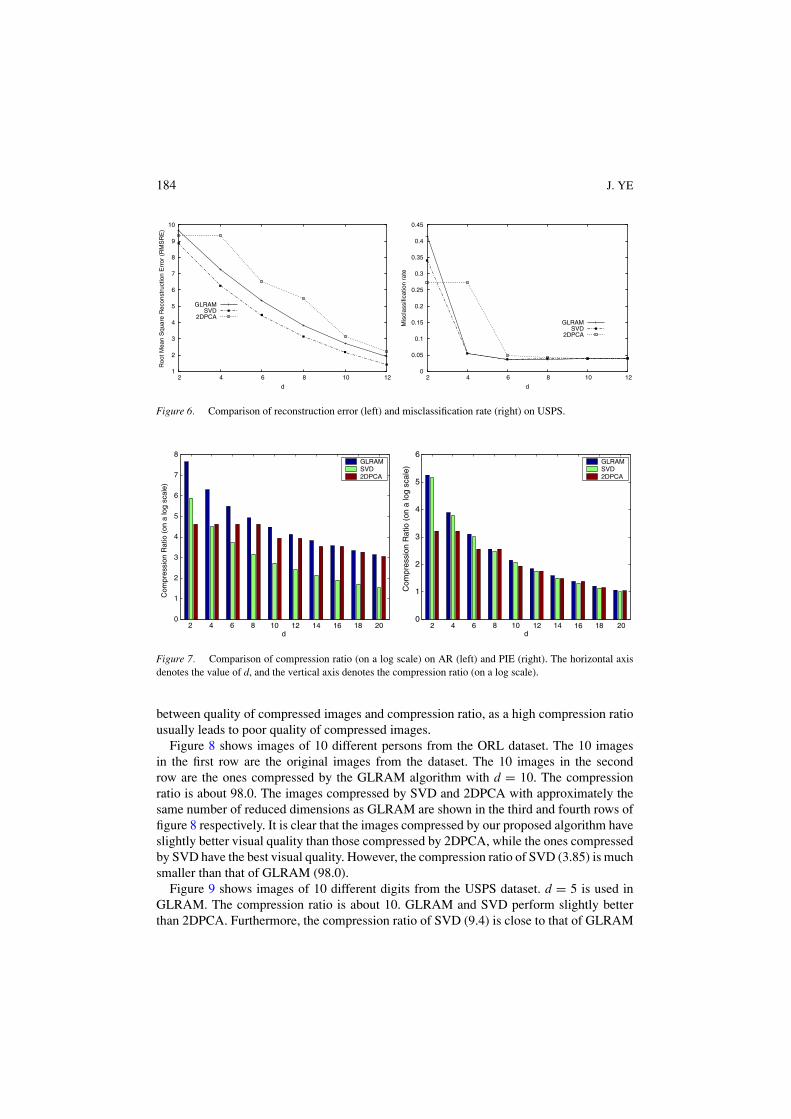
Figures 2–6 show the results on the five image datasets: PIX, ORL, AR, PIE, and USPSrespectively. The horizontal axis denotes the value of d, and the vertical axis denotesthe RMSRE value (left graph) and misclassification rate (right graph). Figure 7 showsthe compression ratios of all algorithms on AR (left graph) and PIE (right graph), tworepresentatives of all image datasets in Table 3.

The main observations include:

0 1 22 37.5

8

8.5

9

9.5

Number of iterations

RM

SR

E (

on a

log

scal

e)

0 10 20 30 40 50 60 70 80 90 1008.8964

8.8965

8.8966

8.8967

8.8968

8.8969

8.897

8.8971

8.8972

Number of iterations

RM

SR

E (

on a

log

scal

e)

Figure 1. Sensitivity of GLRAM to the choice of the initial L0 on ORL (left) and RAND (right). The ten curvescorrespond to the ten runs with different initial L0’s. The horizontal axis is the number of iterations and the verticalaxis is the RMSRE value (on a log scale).

182 J. YE

– As d increases, the reconstruction error by GLRAM decreases monotonically for all cases,while the misclassification rate decreases monotonically in most cases. The same trendcan be observed from other algorithms. Thus choosing a large d in general improves theperformance of GLRAM in reconstruction and classification. However, the computationcost of GLRAM also increases as d increases, as shown in Table 2 (Note that d = �1

= �2). There is a tradeoff between the performance and the computation cost, whenchoosing the best d in GLRAM.

– SVD has the smallest RMSRE value in all cases, while 2DPCA has the largest RMSREvalue in most cases. The large reconstruction error of 2DPCA is due to its poor compres-sion performance, when using only one-sided transformation, as compared to two-sidedtransformation in GLRAM.

– For datasets with a relatively large number of dimensions compared to the number ofdata points, such as the AR datasets, the compression ratio of SVD is much smaller thanothers as shown in figure 7 (left graph). As the number of data points gets as large as inthe PIE dataset, the compression ratio of SVD becomes close to GLRAM, as shown infigure 7 (right graph).

0

100

200

300

400

500

600

700

800

900

1000

2 4 6 8 10 12 14 16 18 20

Roo

t Mea

n S

quar

e R

econ

stru

ctio

n E

rror

(R

MS

RE

)

d

GLRAMSVD

2DPCA

0.02

0.03

0.04

0.05

0.06

0.07

0.08

2 4 6 8 10 12 14 16 18 20

Mis

clas

sific

atio

n ra

te

d

GLRAMSVD

2DPCA

Figure 2. Comparison of reconstruction error (left) and misclassification rate (right) on PIX.

0

500

1000

1500

2000

2500

3000

3500

4000

2 4 6 8 10 12 14 16 18 20

Roo

t Mea

n S

quar

e R

econ

stru

ctio

n E

rror

(R

MS

RE

)

d

GLRAMSVD

2DPCA

0

0.05

0.1

0.15

0.2

0.25

0.3

0.35

2 4 6 8 10 12 14 16 18 20

Mis

clas

sific

atio

n ra

te

d

GLRAMSVD

2DPCA

Figure 3. Comparison of reconstruction error (left) and misclassification rate (right) on ORL.


1000

2000

3000

4000

5000

6000

7000

2 4 6 8 10 12 14 16 18 20

Roo

t Mea

n S

quar

e R

econ

stru

ctio

n E

rror

(R

MS

RE

)

d

GLRAMSVD

2DPCA

0.2

0.3

0.4

0.5

0.6

0.7

0.8

2 4 6 8 10 12 14 16 18 20

Mis

clas

sific

atio

n ra

te

d

GLRAMSVD

2DPCA

Figure 4. Comparison of reconstruction error (left) and misclassification rate (right) on AR.

100

200

300

400

500

600

700

800

900

1000

1100

2 4 6 8 10 12 14 16 18 20

Roo

t Mea

n S

quar

e R

econ

stru

ctio

n E

rror

(R

MS

RE

)

d

GLRAMSVD

2DPCA

0

0.1

0.2

0.3

0.4

0.5

0.6

0.7

0.8

2 4 6 8 10 12 14 16 18 20

Mis

clas

sific

atio

n ra

te

d

GLRAMSVD

2DPCA

Figure 5. Comparison of reconstruction error (left) and misclassification rate (right) on PIE.

– GLRAM is competitive with SVD for classification in most cases, even though GLRAMhas larger RMSRE values. This may be related to the fact that GLRAM is able to utilizethe locality information (e.g. smoothness in an image) intrinsic in the image, which leadsto good classification performance. We apply GLRAM to datasets without any localityproperty, such as text documents and gene expression data, by reshaping each vector as amatrix. GLRAM performs quite poorly in both the reconstruction error and classificationas compared to SVD.

– The reconstruction error and misclassification rate on AR are much higher than those ofother image datasets. This may be related to the large within-class variances on AR, dueto the presence of sun glasses and scarves, as mentioned in Section 5.1.

5.5. Compression effectiveness

In this experiment, we examine the quality of the images compressed by the proposed algo-rithm and compare it with SVD and 2DPCA. Image compression is commonly applied as apre-processing step for storage and transmission of large image data. There exists a tradeoff

184 J. YE

1

2

3

4

5

6

7

8

9

10

2 4 6 8 10 12

Roo

t Mea

n S

quar

e R

econ

stru

ctio

n E

rror

(R

MS

RE

)

d

GLRAMSVD

2DPCA

0

0.05

0.1

0.15

0.2

0.25

0.3

0.35

0.4

0.45

2 4 6 8 10 12

Mis

clas

sific

atio

n ra

te

d

GLRAMSVD

2DPCA

Figure 6. Comparison of reconstruction error (left) and misclassification rate (right) on USPS.

2 4 6 8 10 12 14 16 18 200

1

2

3

4

5

6

7

8

d

Com

pres

sion

Rat

io (

on a

log

scal

e)

GLRAMSVD2DPCA

2 4 6 8 10 12 14 16 18 200

1

2

3

4

5

6

d

Com

pres

sion

Rat

io (

on a

log

scal

e)

GLRAMSVD2DPCA

Figure 7. Comparison of compression ratio (on a log scale) on AR (left) and PIE (right). The horizontal axisdenotes the value of d, and the vertical axis denotes the compression ratio (on a log scale).

between quality of compressed images and compression ratio, as a high compression ratiousually leads to poor quality of compressed images.

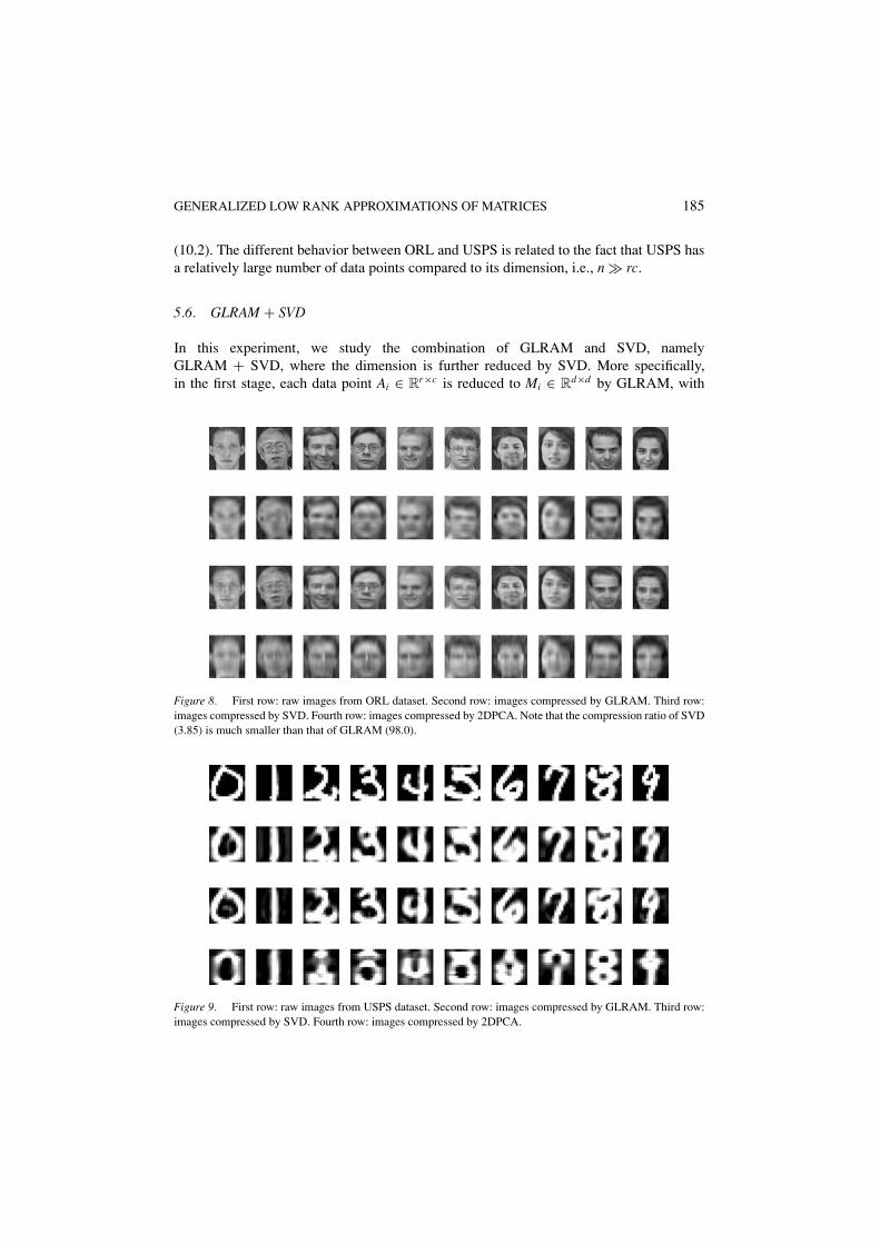
Figure 8 shows images of 10 different persons from the ORL dataset. The 10 imagesin the first row are the original images from the dataset. The 10 images in the secondrow are the ones compressed by the GLRAM algorithm with d = 10. The compressionratio is about 98.0. The images compressed by SVD and 2DPCA with approximately thesame number of reduced dimensions as GLRAM are shown in the third and fourth rows offigure 8 respectively. It is clear that the images compressed by our proposed algorithm haveslightly better visual quality than those compressed by 2DPCA, while the ones compressedby SVD have the best visual quality. However, the compression ratio of SVD (3.85) is muchsmaller than that of GLRAM (98.0).

Figure 9 shows images of 10 different digits from the USPS dataset. d = 5 is used inGLRAM. The compression ratio is about 10. GLRAM and SVD perform slightly betterthan 2DPCA. Furthermore, the compression ratio of SVD (9.4) is close to that of GLRAM


(10.2). The different behavior between ORL and USPS is related to the fact that USPS hasa relatively large number of data points compared to its dimension, i.e., n rc.

5.6. GLRAM + SVD

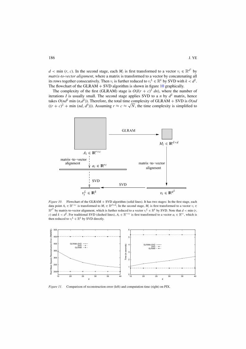
In this experiment, we study the combination of GLRAM and SVD, namelyGLRAM + SVD, where the dimension is further reduced by SVD. More specifically,in the first stage, each data point Ai ∈ R

r×c is reduced to Mi ∈ Rd×d by GLRAM, with

Figure 8. First row: raw images from ORL dataset. Second row: images compressed by GLRAM. Third row:images compressed by SVD. Fourth row: images compressed by 2DPCA. Note that the compression ratio of SVD(3.85) is much smaller than that of GLRAM (98.0).

Figure 9. First row: raw images from USPS dataset. Second row: images compressed by GLRAM. Third row:images compressed by SVD. Fourth row: images compressed by 2DPCA.

186 J. YE

d < min (r, c). In the second stage, each Mi is first transformed to a vector vi ∈ Rd2

bymatrix-to-vector alignment, where a matrix is transformed to a vector by concatenating allits rows together consecutively. Then vi is further reduced to vi

L ∈ Rk by SVD with k < d2.

The flowchart of the GLRAM + SVD algorithm is shown in figure 10 graphically.The complexity of the first (GLRAM) stage is O(I(r + c)2 dn), where the number of

iterations I is usually small. The second stage applies SVD to a n by d2 matrix, hencetakes O(nd2 min (n,d2)). Therefore, the total time complexity of GLRAM + SVD is O(nd((r + c)2 + min (nd, d3))). Assuming r ≈ c ≈ √

N , the time complexity is simplified to

Figure 10. Flowchart of the GLRAM + SVD algorithm (solid lines). It has two stages: In the first stage, eachdata point Ai ∈ R

r×c is transformed to Mi ∈ Rd×d ; In the second stage, Mi is first transformed to a vector vi ∈

Rd2

by matrix-to-vector alignment, which is further reduced to a vector viL ∈ R

k by SVD. Note that d < min (r,c) and k < d2. For traditional SVD (dashed lines), Ai ∈ R

r×c is first transformed to a vector ai ∈ Rrc , which is

then reduced to viL ∈ R

k by SVD directly.

200

250

300

350

400

450

500

15 20 25 30 35 40

Roo

t Mea

n S

quar

e R

econ

stru

ctio

n E

rror

(R

MS

RE

)

d

GLRAM+SVDSVD

GLRAM

0

1

2

3

4

5

6

15 20 25 30 35 40

Tim

e (in

sec

onds

)

d

GLRAM+SVDSVD

GLRAM

Figure 11. Comparison of reconstruction error (left) and computation time (right) on PIX.


1300

1400

1500

1600

1700

1800

1900

2000

15 20 25 30 35 40

Roo

t Mea

n S

quar

e R

econ

stru

ctio

n E

rror

(R

MS

RE

)

d

GLRAM+SVDSVD

GLRAM

0

1

2

3

4

5

6

7

8

9

15 20 25 30 35 40

Tim

e (in

sec

onds

)

d

GLRAM+SVDSVD

GLRAM

Figure 12. Comparison of reconstruction error (left) and computation time (right) on ORL.

2300

2400

2500

2600

2700

2800

2900

3000

15 20 25 30 35 40

Roo

t Mea

n S

quar

e R

econ

stru

ctio

n E

rror

(R

MS

RE

)

d

GLRAM+SVDSVD

GLRAM

0

10

20

30

40

50

60

70

80

90

15 20 25 30 35 40

Tim

e (in

sec

onds

)

d

GLRAM+SVDSVD

GLRAM

Figure 13. Comparison of reconstruction error (left) and computation time (right) on AR.

O(nd (N + min (nd, d3))). Note that both the GLRAM and SVD stages in GLRAM + SVDhave much smaller computation costs than SVD, especially when d is small. (Note that thecost of SVD on an n × N matrix is O(nNmin (n, N)).)

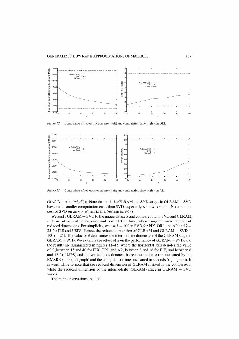
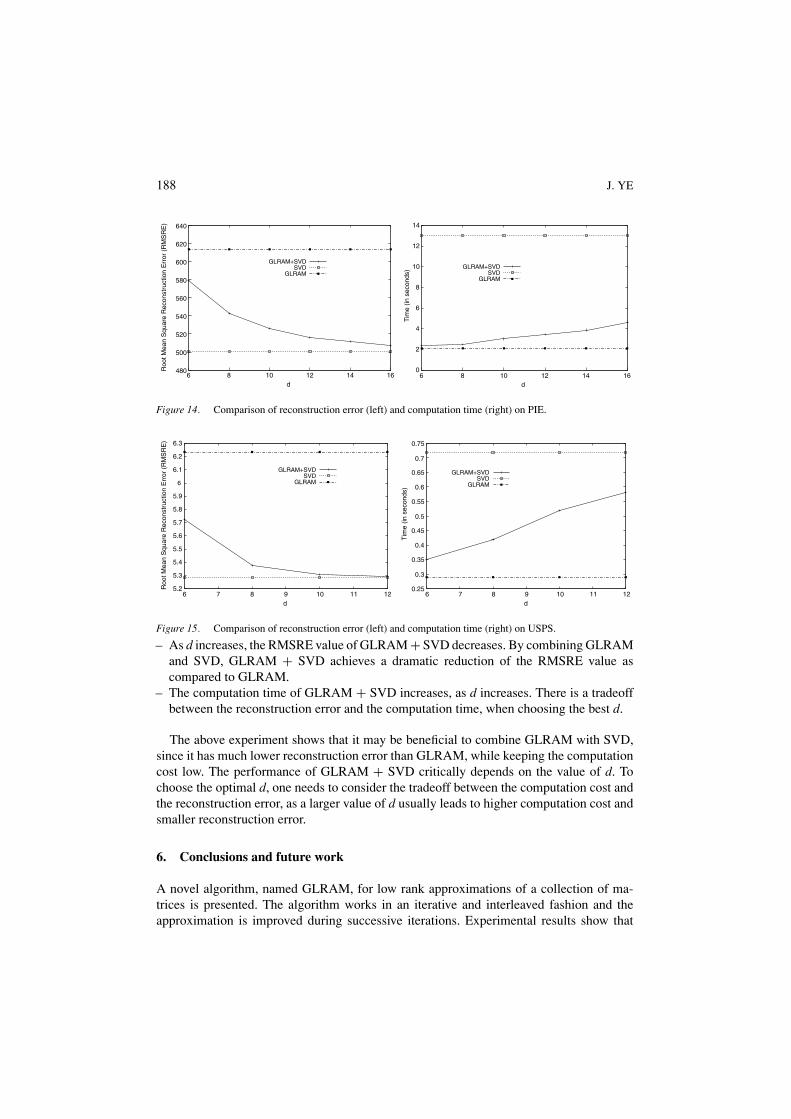
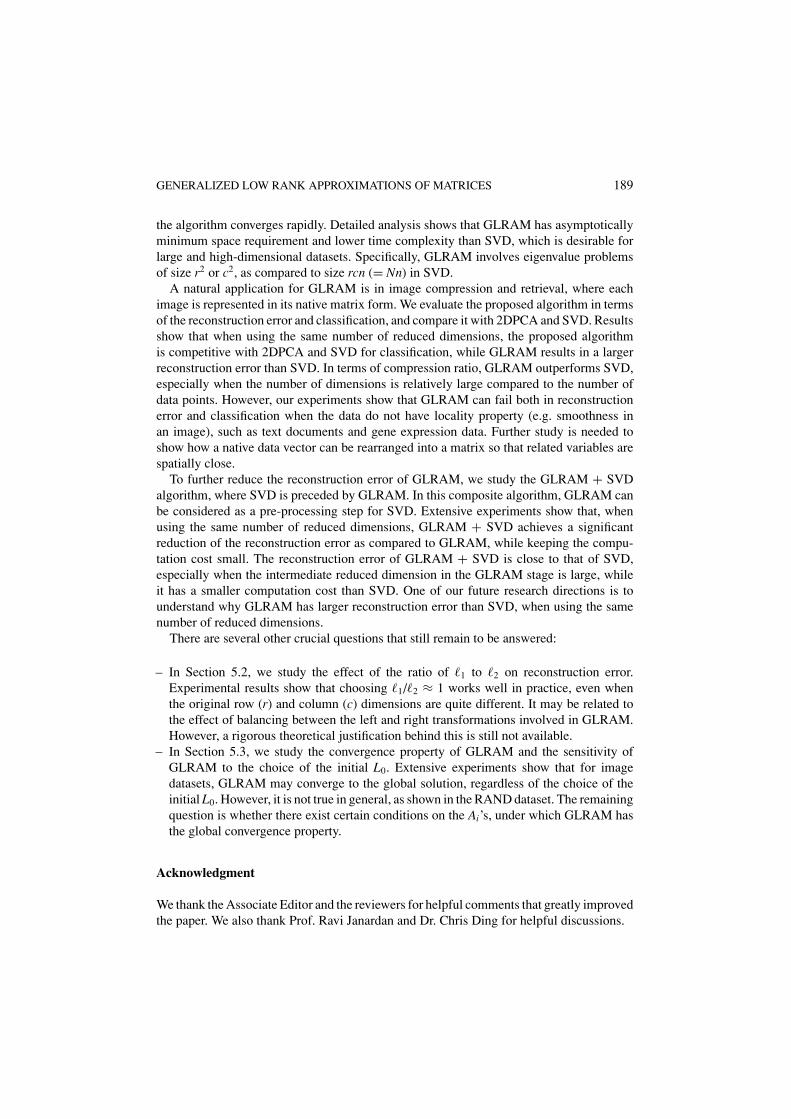
We apply GLRAM + SVD to the image datasets and compare it with SVD and GLRAMin terms of reconstruction error and computation time, when using the same number ofreduced dimensions. For simplicity, we use k = 100 in SVD for PIX, ORL and AR and k =25 for PIE and USPS. Hence, the reduced dimension of GLRAM and GLRAM + SVD is100 (or 25). The value of d determines the intermediate dimension of the GLRAM stage inGLRAM + SVD. We examine the effect of d on the performance of GLRAM + SVD, andthe results are summarized in figures 11–15, where the horizontal axis denotes the valueof d (between 15 and 40 for PIX, ORL and AR, between 6 and 16 for PIE, and between 6and 12 for USPS) and the vertical axis denotes the reconstruction error, measured by theRMSRE value (left graph) and the computation time, measured in seconds (right graph). Itis worthwhile to note that the reduced dimension of GLRAM is fixed in the comparison,while the reduced dimension of the intermediate (GLRAM) stage in GLRAM + SVDvaries.

The main observations include:

188 J. YE

480

500

520

540

560

580

600

620

640

6 8 10 12 14 16

Roo

t Mea

n S

quar

e R

econ

stru

ctio

n E

rror

(R

MS

RE

)

d

GLRAM+SVDSVD

GLRAM

0

2

4

6

8

10

12

14

6 8 10 12 14 16

Tim

e (in

sec

onds

)

d

GLRAM+SVDSVD

GLRAM

Figure 14. Comparison of reconstruction error (left) and computation time (right) on PIE.

5.2

5.3

5.4

5.5

5.6

5.7

5.8

5.9

6

6.1

6.2

6.3

6 7 8 9 10 11 12

Roo

t Mea

n S

quar

e R

econ

stru

ctio

n E

rror

(R

MS

RE

)

d

GLRAM+SVDSVD

GLRAM

0.25

0.3

0.35

0.4

0.45

0.5

0.55

0.6

0.65

0.7

0.75

6 7 8 9 10 11 12

Tim

e (in

sec

onds

)

d

GLRAM+SVDSVD

GLRAM

Figure 15. Comparison of reconstruction error (left) and computation time (right) on USPS.

– As d increases, the RMSRE value of GLRAM + SVD decreases. By combining GLRAMand SVD, GLRAM + SVD achieves a dramatic reduction of the RMSRE value ascompared to GLRAM.

– The computation time of GLRAM + SVD increases, as d increases. There is a tradeoffbetween the reconstruction error and the computation time, when choosing the best d.

The above experiment shows that it may be beneficial to combine GLRAM with SVD,since it has much lower reconstruction error than GLRAM, while keeping the computationcost low. The performance of GLRAM + SVD critically depends on the value of d. Tochoose the optimal d, one needs to consider the tradeoff between the computation cost andthe reconstruction error, as a larger value of d usually leads to higher computation cost andsmaller reconstruction error.

6. Conclusions and future work

A novel algorithm, named GLRAM, for low rank approximations of a collection of ma-trices is presented. The algorithm works in an iterative and interleaved fashion and theapproximation is improved during successive iterations. Experimental results show that


the algorithm converges rapidly. Detailed analysis shows that GLRAM has asymptoticallyminimum space requirement and lower time complexity than SVD, which is desirable forlarge and high-dimensional datasets. Specifically, GLRAM involves eigenvalue problemsof size r2 or c2, as compared to size rcn (= Nn) in SVD.

A natural application for GLRAM is in image compression and retrieval, where eachimage is represented in its native matrix form. We evaluate the proposed algorithm in termsof the reconstruction error and classification, and compare it with 2DPCA and SVD. Resultsshow that when using the same number of reduced dimensions, the proposed algorithmis competitive with 2DPCA and SVD for classification, while GLRAM results in a largerreconstruction error than SVD. In terms of compression ratio, GLRAM outperforms SVD,especially when the number of dimensions is relatively large compared to the number ofdata points. However, our experiments show that GLRAM can fail both in reconstructionerror and classification when the data do not have locality property (e.g. smoothness inan image), such as text documents and gene expression data. Further study is needed toshow how a native data vector can be rearranged into a matrix so that related variables arespatially close.

To further reduce the reconstruction error of GLRAM, we study the GLRAM + SVDalgorithm, where SVD is preceded by GLRAM. In this composite algorithm, GLRAM canbe considered as a pre-processing step for SVD. Extensive experiments show that, whenusing the same number of reduced dimensions, GLRAM + SVD achieves a significantreduction of the reconstruction error as compared to GLRAM, while keeping the compu-tation cost small. The reconstruction error of GLRAM + SVD is close to that of SVD,especially when the intermediate reduced dimension in the GLRAM stage is large, whileit has a smaller computation cost than SVD. One of our future research directions is tounderstand why GLRAM has larger reconstruction error than SVD, when using the samenumber of reduced dimensions.

There are several other crucial questions that still remain to be answered:

– In Section 5.2, we study the effect of the ratio of �1 to �2 on reconstruction error.Experimental results show that choosing �1/�2 ≈ 1 works well in practice, even whenthe original row (r) and column (c) dimensions are quite different. It may be related tothe effect of balancing between the left and right transformations involved in GLRAM.However, a rigorous theoretical justification behind this is still not available.

– In Section 5.3, we study the convergence property of GLRAM and the sensitivity ofGLRAM to the choice of the initial L0. Extensive experiments show that for imagedatasets, GLRAM may converge to the global solution, regardless of the choice of theinitial L0. However, it is not true in general, as shown in the RAND dataset. The remainingquestion is whether there exist certain conditions on the Ai’s, under which GLRAM hasthe global convergence property.

Acknowledgment

We thank the Associate Editor and the reviewers for helpful comments that greatly improvedthe paper. We also thank Prof. Ravi Janardan and Dr. Chris Ding for helpful discussions.

190 J. YE

This research is sponsored, in part, by the Army High Performance Computing ResearchCenter under the auspices of the Department of the Army, Army Research Laboratory coop-erative agreement number DAAD19-01-2-0014, the content of which does not necessarilyreflect the position or the policy of the government, and no official endorsement shouldbe inferred. Support Fellowships from Guidant Corporation and from the Department ofComputer Science & Engineering, at the University of Minnesota, Twin Cities is gratefullyacknowledged.

Notes

1. Here the compression ratio means the percentage of space saved by the low rank approximations to store thedata. Details can be found in Sections 2 and 3.

2. http://peipa.essex.ac.uk/ipa/pix/faces/manchester/test-hard/3. http://www.uk.research.att.com/facedatabase.html4. http://rvl1.ecn.purdue.edu/∼aleix/aleix face DB.html5. http://www.ri.cmu.edu/projects/project 418.html6. http://www-stat-class.stanford.edu/∼tibs/ElemStatLearn/data.html

References

Achlioptas, D., & McSherry, F. (2001). Fast computation of low rank matrix approximations. In ACM STOCConference Proceedings (pp. 611–618).

Aggarwal, C. C. (2001). On the effects of dimensionality reduction on high dimensional similarity search. In ACMPODS Conference Proceedings (pp. 256–266).

Averbuch, A., Lazar, D., & Israeli, M. (1996). Image compression using wavelet transform and multiresolutiondecomposition. IEEE Transactions on Image Processing, 5:1, 4–15.

Berry, M., Dumais, S., & O’Brie, G. (1995). Using linear algebra for intelligent information retrieval. SIAMReview, 37, 573–595.

Bjork, A., & Golub, G. (1973). Numerical methods for computing angles between linear subspaces. Mathematicsof Computation, 27:123, 579–594.

Brand, M. (2002). Incremental singular value decomposition of uncertain data with missing values. In ECCVConference Proceedings (pp. 707–720).

Castelli, V., Thomasian, A., & Li, C.-S. (2003). CSVD: Clustering and singular value decomposition for approx-imate similarity searches in high dimensional space. IEEE Transactions on Knowledge and Data Engineering,15:3, 671–685.

Deerwester, S., Dumais, S., Furnas, G., Landauer, T., & Harshman, R. (1990). Indexing by latent semantic analysis.Journal of the Society for Information Science, 41, 391–407.

Dhillon, I., & Modha, D. (2001). Concept decompositions for large sparse text data using clustering. MachineLearning, 42, 143–175.

Drineas, P., Frieze, A., Kannan, R., Vempala, S., & Vinay, V. (1999). Clustering in large graphs and matrices. InACM SODA Conference Proceedings (pp. 291–299).

Duda, R., Hart, P., & Stork, D. (2000). Pattern classification. Wiley.Edelman, A., Arias, T. A., & Smith, S. T. (1998). The geometry of algorithms with orthogonality constraints.

SIAM Journal on Matrix Analysis and Applications, 20:2, 303–353.Frieze, A., Kannan, R., & Vempala, S. (1998). Fast monte-carlo algorithms for finding low-rank approximations.

In ACM FOCS Conference Proceedings (pp. 370–378).Fukunaga, K. (1990). Introduction to statistical pattern classification. San Diego, California, USA: Academic

Press.Golub, G. H., & Van Loan, C. F. (1996). Matrix computations, 3rd edition. Baltimore, MD, USA: The Johns

Hopkins University Press.


Gu, M., & Eisenstat, S. C. (1993). A fast and stable algorithm for updating the singular value decomposition.Technical Report YALEU/DCS/RR-966, Department of Computer Science, Yale University.

Kanth, K. V. R., Agrawal, D., Abbadi, A. E., & Singh, A. (1998). Dimensionality reduction for similarity searchingin dynamic databases. In ACM SIGMOD Conference Proceedings (pp. 166–176).

Kleinberg, J., & Tomkins, A. (1999). Applications of linear algebra in information retrieval and hypertext analysis.In ACM PODS Conference Proceedings (pp. 185–193).

Kolda, T. G. (2001). Orthogonal tensor decompositions. SIAM Journal on Matrix Analysis and Applications, 23:1,243–255.

Martinez, A., & Benavente, R. (1998). The AR face database. Technical Report CVC Tech. Report No. 24.Papadimitriou, C. H., Tamaki, H., Raghavan, P., & Vempala, S. (1998). Latent semantic indexing: A probabilistic

analysis. In PODS Conference Proceedings (pp. 159–168).Samaria, F., & Harter, A. (1994). Parameterisation of a stochastic model for human face identification. In

Proceedings of 2nd IEEE Workshop on Applications of Computer Vision, Sarasota FL (pp. 138–142).Shashua, A., & Levin, A. (2001). Linear image coding for regression and classification using the tensor-rank

principle. In CVPR Conference Proceedings (pp. 42–49).Sim, T., Baker, S., & Bsat, M. (2004). The CMU pose, illumination, and expression (PIE) database. IEEE

Transactions on Pattern Analysis and Machine Intelligence, 25:12, 1615–1618.Srebro, N., & Jaakkola, T. (2003). Weighted low-rank approximations. In ICML Conference Proceedings (pp.

720–727).Vasilescu, M. A. O., & Terzopoulos, D. (2002). Multilinear analysis of image ensembles: Tensorfaces. In ECCV

Conference Proceedings (pp. 447–460).Yang, J., Zhang, D., Frangi, A., & Yang, J. (2004). Two-dimensional PCA: A new approach to appearance-based

face representation and recognition. IEEE Transactions on Pattern Analysis and Machine Intelligence, 5:1,131–137.

Zhang, T., & Golub, G. H. (2001). Rank-one approximation to high order tensors. SIAM Journal on MatrixAnalysis and Applications, 5:2, 534–550.

Received May 25, 2004Revised June 28, 2005Accepted June 28, 2005

Documents

Generalized Low Rank Approximations of Matrices