at SciVerse ScienceDirect

Renewable Energy 44 (2012) 72e79

Contents lists available

Renewable Energy

journal homepage: www.elsevier .com/locate/renene

Generic maximum power point tracking controller for small-scale wind turbines

M. Narayana a,*, G.A. Putrus a, M. Jovanovic a, P.S. Leung a, S. McDonald b

aNorthumbria University, Ellison Place, Newcastle Upon Tyne, UKbNew and Renewable Energy Centre (NaREC), Blyth, UK

a r t i c l e i n f o

Article history:Received 26 June 2011Accepted 30 December 2011Available online 31 January 2012

Keywords:Wind energy conversion systemsWind rotorMaximum power point tracking controlAdaptive controlFuzzy Logic

* Corresponding author. Northumbria University, ScEllison Place, Newcastle Upon Tyne NE1 8ST, Newcast

E-mail addresses: mahinsasa@yahoo.com (M.unn.ac.uk (G.A. Putrus), milutin.jovanovic@unn.ac.uunn.ac.ukand (P.S. Leung), steve.mcdonald@narec.co.u

0960-1481/$ e see front matter � 2012 Elsevier Ltd.doi:10.1016/j.renene.2011.12.015

a b s t r a c t

The output power of a wind energy conversion system (WECS) is maximized if the wind rotor is driven atan optimal rotational speed for a particular wind speed. To achieve this, a Maximum Power PointTracking (MPPT) controller is usually used. A successful implementation of the MPPT controller requiresknowledge of the turbine dynamics and instantaneous measurements of the wind speed and rotor speed.To obtain the optimal operating point, rotor-generator characteristics should be known and these aredifferent from one system to another. Therefore, there is a need for an efficient universal MPPT controllerfor WECS to operate without predetermined characteristics. MPPT control of WECSs becomes difficultdue to fluctuation of wind speed and wind rotor inertia. This issue is analyzed in the paper, and anAdaptive Filter together with a Fuzzy Logic based MPPT controller suitable for small-scale WECSs isproposed. The proposed controller can be implemented without predetermined WECS characteristics.

� 2012 Elsevier Ltd. All rights reserved.

1. Introduction

Variable-speed fixed-pitch (VSFP) wind energy conversionsystems (WECSs) are generally more efficient compared to fixed-speed counterparts, and hence are becoming increasinglypopular, particularly in small-scale applications. Wind turbineswith variable-pitch control are generally costly and complex.Typically, variable-speed wind turbines are aerodynamicallycontrolled, usually by using power electronics, to regulate the tor-que and speed of the turbine in order to maximize the outputpower. Therefore, VSFP approach is becomingmore popular for lowcost construction, and is the most common scheme for small windturbines. In this scheme, aMaximum Power Point Tracker (MPPT) isused to control the restoring torque of the electrical generator foroptimum system operation [1]. Accordingly, the performance ofa VSFP wind turbine could be optimized without the need fora complex aerodynamic control. The maximum output power fromthe turbine is usually obtained by controlling the system such thatthe relevant points of wind rotor curve and electrical generatoroperating characteristic coincide. In order to achieve this, it isnecessary to drive the turbine at optimal rotor speeds for a partic-ular wind speed profile.

hool of CEIS, Ellison Building,le Upon Tyne, UK.Narayana), ghanim.putrus@k (M. Jovanovic), ps.leung@k (S. McDonald).

All rights reserved.

Techniques that employ wind sensors generally perform wellwith wind speed variations, as the control system responds tovariation inwind conditions [2,3]. However, in practice it is difficultto accurately measure the wind speed by an anemometer installedclose to the wind turbine, as the latter is exposed to different forcesdue to wake rotation. Normally, wind rotor blades experienceconning and flapping effects due to wind forces. Wind speed variesacross the swept area of the wind rotor as a result of the yawbehaviour. Accordingly, wind rotor dynamics vary and becomedifficult to predict in real systems. Therefore, it would be useful toimplement a sensorless control strategy, which is proposed in thisstudy, for small-scale wind turbine systems that operate withoutpredetermined turbine characteristics.

2. Aerodynamic characteristics of the wind rotor

Based on the wind turbine aerodynamic behaviour, the amountof power that a wind turbine can capture from the kinetic energycontained in the wind is given as [4]:

Pa ¼ 12$r$p$R2r $v

3$Cp (1)

Where Pa is the captured power by the wind rotor, r is the airdensity (kg/m3), R is the radius of the rotor (m) and v is the speed ofthe incident wind (m/s). Cp is the power coefficient which fora given wind rotor depends on the pitch angle of the wind rotorblades and on the tip speed ratio (l) defined as:

Nomenclature

Dd “Fuzzy set” outputhopt Optimal generator efficiencyFd, Fq d-q axis flux linkagesl Tip speed ratior Air densityu Angular velocity of the wind rotorus Angular frequency of the stator voltageCp Power coefficient of the wind rotorCp_opt Power coefficient at optimal operating conditionCt Torque coefficientD Duty ratio (range, 0e1)id,q PMG stator d-q currentsVG The voltage at the generator sideIG The current flow from the generator sideVB The voltage at the d.c. bus

IB The current flow towards the d.c. busJ Momentum of inertia of rotating partsLd,q 3-phase d-q inductancesPa Aerodynamic power captured by the wind rotorPE Output power of the WECS generatorPl Electrical and friction lossesPWR Power delivered by the wind rotor to the generatorPMG Permanent Magnet GeneratorR Generator winding resistanceRr Radius of the wind rotorTe Electromagnetic torque of the PMGTfriction Torque due to system friction lossesud,q PMG stator d-q voltagesv Incident wind speedVSFP Variable-speed Fixed-PitchWECS Wind Energy Conversion System

M. Narayana et al. / Renewable Energy 44 (2012) 72e79 73

l ¼ u$Rrv

(2)

where u is the angular velocity of the rotor (rad/s).The wind rotor aerodynamic characteristics are usually repre-

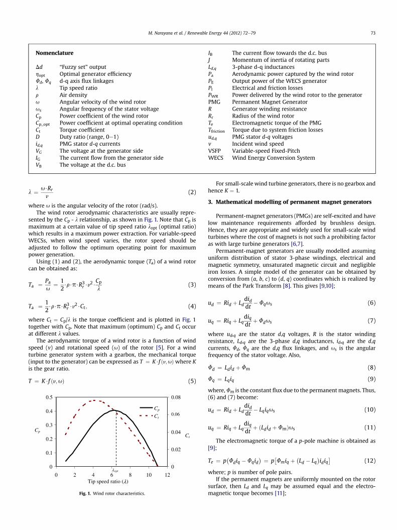
sented by the Cp - l relationship, as shown in Fig. 1. Note that Cp ismaximum at a certain value of tip speed ratio lopt (optimal ratio)which results in a maximum power extraction. For variable-speedWECSs, when wind speed varies, the rotor speed should beadjusted to follow the optimum operating point for maximumpower generation.

Using (1) and (2), the aerodynamic torque (Ta) of a wind rotorcan be obtained as:

Ta ¼ Pau

¼ 12$r$p$R3r $v

2$Cpl

(3)

Ta ¼ 12$r$p$R3r $v

2$Ct; (4)

where Ct ¼ Cp/l is the torque coefficient and is plotted in Fig. 1together with Cp. Note that maximum (optimum) Cp and Ct occurat different l values.

The aerodynamic torque of a wind rotor is a function of windspeed (v) and rotational speed (u) of the rotor [5]. For a windturbine generator system with a gearbox, the mechanical torque(input to the generator) can be expressed as T ¼ K$f ðv;uÞ where Kis the gear ratio.

T ¼ K$f ðv;uÞ (5)

0

0.1

0.2

0.3

0.4

0.5

0 2 4 6 8 10 12Tip speed ratio (

λ

λ)

Cp

0

0.02

0.04

0.06

0.08

Ct

Cp

Ct

opt

Fig. 1. Wind rotor characteristics.

For small-scale wind turbine generators, there is no gearbox andhence K ¼ 1.

3. Mathematical modelling of permanent magnet generators

Permanent-magnet generators (PMGs) are self-excited and havelow maintenance requirements afforded by brushless design.Hence, they are appropriate and widely used for small-scale windturbines where the cost of magnets is not such a prohibiting factoras with large turbine generators [6,7].

Permanent-magnet generators are usually modelled assuminguniform distribution of stator 3-phase windings, electrical andmagnetic symmetry, unsaturated magnetic circuit and negligibleiron losses. A simple model of the generator can be obtained byconversion from (a, b, c) to (d, q) coordinates which is realized bymeans of the Park Transform [8]. This gives [9,10];

ud ¼ Rid þ Lddiddt

� Fqus (6)

uq ¼ Riq þ Lqdiqdt

þ Fdus (7)

where ud,q are the stator d,q voltages, R is the stator windingresistance, Ld,q are the 3-phase d,q inductances, id,q are the d,qcurrents, Fd, Fq are the d,q flux linkages, and us is the angularfrequency of the stator voltage. Also,

Fd ¼ Ldid þ Fm (8)

Fq ¼ Lqiq (9)

where,Fm is the constant flux due to the permanentmagnets. Thus,(6) and (7) become:

ud ¼ Rid þ Lddiddt

� Lqiqus (10)

uq ¼ Riq þ Lqdiqdt

þ ðLdid þ FmÞus (11)

The electromagnetic torque of a p-pole machine is obtained as[9];

Te ¼ p�Fdiq � Fqid

� ¼ p�Fmiq þ

�Ld � Lq

�idiq�

(12)

where; p is number of pole pairs.If the permanent magnets are uniformly mounted on the rotor

surface, then Ld and Lq may be assumed equal and the electro-magnetic torque becomes [11];

0

50

100

150

200

250

0 10 20 30 40 50 60

Rotational speed (rad/s)

Pow

er (

W)

0

1

2

3

4

5

6

7

8

Tor

que

(Nm

)

Input power curves of the generator

Wind rotor torque curve

Wind rotor aerodynamic power curve

Optimum operating point

Maximum power point of the wind rotor power curve

Electrical output power curve

Maximum output power point

Generator power loss

Fig. 2. Operating point of the wind power system.

Rotational speed

V1

V2

Optimum line

Eff

ectiv

e po

wer

ω2 ω1

Wind

speeds

Fig. 3. Function of MPPT mechanism.

M. Narayana et al. / Renewable Energy 44 (2012) 72e7974

Te ¼ pFmiq (13)

Note that the stator voltage frequency (us) is proportional to theshaft rotational speed (u), i.e. us ¼ p.u.

The electromagnetic torque developed by the generator isa function of the generator current (IG), magnetic flux linkage andnumber of pole pairs [12,13]. For a particular generator, themagnetic flux linkage and number of pole pairs are fixed parame-ters. Hence, TefIG. Therefore, the electromagnetic torque ofa generator (Te) can be varied by controlling the PMG current. Themain power loss in the PMG may be expressed as 3$I2GR. This lossincreases at higher torques (as IG is higher) and this operation isassociated with low rotational speed and low voltage for the sameoutput power. Therefore, variation of the power loss needs to beconsidered for maximum power tracking, as described in thefollowing section.

4. Control strategies

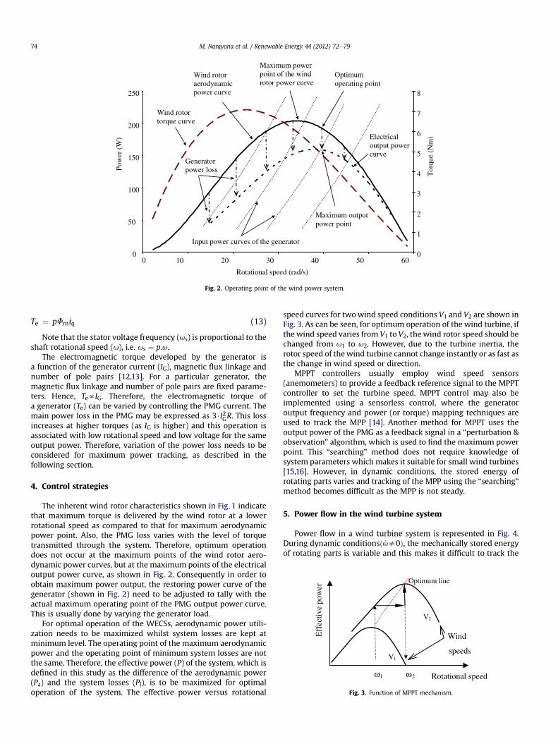
The inherent wind rotor characteristics shown in Fig. 1 indicatethat maximum torque is delivered by the wind rotor at a lowerrotational speed as compared to that for maximum aerodynamicpower point. Also, the PMG loss varies with the level of torquetransmitted through the system. Therefore, optimum operationdoes not occur at the maximum points of the wind rotor aero-dynamic power curves, but at the maximum points of the electricaloutput power curve, as shown in Fig. 2. Consequently in order toobtain maximum power output, the restoring power curve of thegenerator (shown in Fig. 2) need to be adjusted to tally with theactual maximum operating point of the PMG output power curve.This is usually done by varying the generator load.

For optimal operation of the WECSs, aerodynamic power utili-zation needs to be maximized whilst system losses are kept atminimum level. The operating point of the maximum aerodynamicpower and the operating point of minimum system losses are notthe same. Therefore, the effective power (P) of the system, which isdefined in this study as the difference of the aerodynamic power(Pa) and the system losses (Pl), is to be maximized for optimaloperation of the system. The effective power versus rotational

speed curves for twowind speed conditions V1 and V2 are shown inFig. 3. As can be seen, for optimum operation of the wind turbine, ifthewind speed varies from V1 to V2, thewind rotor speed should bechanged from u1 to u2. However, due to the turbine inertia, therotor speed of thewind turbine cannot change instantly or as fast asthe change in wind speed or direction.

MPPT controllers usually employ wind speed sensors(anemometers) to provide a feedback reference signal to the MPPTcontroller to set the turbine speed. MPPT control may also beimplemented using a sensorless control, where the generatoroutput frequency and power (or torque) mapping techniques areused to track the MPP [14]. Another method for MPPT uses theoutput power of the PMG as a feedback signal in a “perturbation &observation” algorithm, which is used to find the maximum powerpoint. This “searching” method does not require knowledge ofsystem parameters which makes it suitable for small wind turbines[15,16]. However, in dynamic conditions, the stored energy ofrotating parts varies and tracking of the MPP using the “searching”method becomes difficult as the MPP is not steady.

5. Power flow in the wind turbine system

Power flow in a wind turbine system is represented in Fig. 4.During dynamic conditionsð _us0Þ, the mechanically stored energyof rotating parts is variable and this makes it difficult to track the

M. Narayana et al. / Renewable Energy 44 (2012) 72e79 75

MPP (e.g. by using hill-climbed searching methods) from theelectric power as the electrical power output is uncorrelated withthe captured aerodynamic power by the wind rotor. The aero-dynamic torque (Ta) under dynamic conditions is given as:

Ta ¼ _u$J þ Te þ Tfriction (14)

where J is moment of inertia of rotating parts, Te is the electro-magnetic torque of the generator and Tfriction is the torque due tosystem friction losses.

Equation (14) may be rewritten as:

Pa ¼ u$ _u$J þ PE þ Pl (15)

PWR ¼ Pa � u$ _u$J (16)

PE ¼ PWR � Pl (17)

where Pa is the aerodynamic power extracted by the rotor, PWR ispower delivered by the wind rotor to the generator (see Fig. 4), PE isthe output power of the generator, Pl is the electrical and frictionlosses and _u ¼ du=dt. Therefore;

PE ¼ �u$ _u$J þ ðPa � PlÞ (18)

This equation defines the relationship, during dynamic condi-tions, between the electrical output power of the generator (PE), theaerodynamic power extracted by the rotor (Pa) and the mechan-ically stored energy of rotating parts. In this study, an adaptive filteris used to extract the values of (u$ _u$J) and (Pa e Pl) from themeasured values of electrical output power, as described in thefollowing section. The extracted signals are then used as controlsignals for the proposed MPPT to define the optimum operatingpoints.

6. Adaptive filtering

Wind speed-time series data typically exhibit autocorrelation,which can be defined as the degree of dependence on precedingvalues [17]. Therefore, variation of mechanically stored energy inthe rotating parts ðu$ _u$JÞ and electrical output (PE) are time seriesdata. Variation of the rotational speed is mainly dependent on themomentum of inertia of the rotating parts. As given by (18), theelectrical output of the generator is the combination of the effectiveoutput power (PaePl) and the variation of mechanically storedenergy. Accordingly, the wind rotor speed and effective outputpower of the WECS change with the wind speed variations.

In this work, a simulation study (based on real wind data) wasused to examine the correlation between the time series data ofðu$ _uÞ and electrical output. A small wind turbine at the NationalEngineering Research & Development Centre (NERDC) in Sri Lankawas simulated in MATLAB/SIMULINK using measured (actual) wind

Wind

= − = JPP aWR ..ω ω

ω ω ,

Pa = Aerodynamic power extracted by the wind rotor

Input power to the generator

PMG

lossesfriction 2 + = RIP dl

Aerodynamic losses

Generated electric power

PPP − =

Fig. 4. Power flow of the wind turbine.

speed data in turbulent wind conditions. Specifications of thesystem used are given in the Appendix (A).

An “adaptive filter” is a filter that self-adjusts its transfer func-tion according to an optimizing algorithm. The adaptive filter, W, isimplemented using the least mean square algorithm. A blockdiagram of the filter is shown in Fig. 5. An error signal, e(n), iscomputed as e(n) ¼ d(n)�y(n), which measures the differencebetween the output of the adaptive filter [y(n)] and the output of anunknown system [d(n)]. With reference to Fig. 5, assuming that p(n)is uncorrelated with u(n), z(n) and y(n), and that u(n), z(n), y(n) arestatistically stationary and have zero means:

eðnÞ ¼ pðnÞ þ zðnÞ � yðnÞ (19)

Squaring of both sides of (19):

eðnÞ2 ¼ pðnÞ2þ½zðnÞ � yðnÞ�2þ2pðnÞ½zðnÞ � yðnÞ� (20)

Taking expectation of both sides of (20), and realizing that p(n) isuncorrelated with z(n) and y(n)

EheðnÞ2

i¼ E

hpðnÞ2

iþEn½zðnÞ�yðnÞ�2

oþ2EfpðnÞ½zðnÞ�yðnÞ�g ¼ E

hpðnÞ2

iþEn½zðnÞ� yðnÞ�2

o; (21)

as E[z(n)] ¼ 0 and E[y(n)] ¼ 0Adapting the filter to minimize E[e(n)2] will not affect the signal

power E[p(n)2]. Accordingly, the minimum output signal power is,

Emin

heðnÞ2

i¼ E

hpðnÞ2

iþ Emin

n½zðnÞ � yðnÞ�2

o(22)

The signal power E[p(n)2] is unchanged when the filter coeffi-cients are adjusted in error minimization algorithm. Consequently,only the term E{[z(n)�y(n)]2} is minimized in the mean squareerror (MSE) minimization. When the algorithm converges tominimum mean square error (MMSE) solution, y(n) represents thebest estimation of z(n) [18].

Thus z(n)zy(n) since e(n) ¼ p(n)þz(n)�y(n). This implies thate(n)zp(n), where p(n) is the best estimate of the error signal e(n).This argument implies that minimization of MSE entails.

If X(t) and Y(t) are two sets of time series data, the correlationcoefficient rx,Y between them is given as;

Correlation(X,Y) ¼ rxY

¼PN

t¼1

�XðtÞ � X

��YðtÞ � Y

�ffiffiffiffiffiffiffiffiffiffiffiffiffiffiffiffiffiffiffiffiffiffiffiffiffiffiffiffiffiffiffiffiffiffiffiffiffiffiffiffiffiffiffiffiffiffiffiffiffiffiffiffiffiffiffiffiffiffiffiffiffiffiffiffiffiffiffiffiffiffiffiffiffiffiffiffiffiffiffiffiffiPN

t¼1

�XðtÞ � X

�2PNt¼1

�YðtÞ � Y

�2s (23)

where X ¼ PNt¼1 XðtÞ=N and, Y ¼ PN

t¼1 YðtÞ=NUsing 2500 data sets obtained from the simulation study, the

correlation coefficients between the time series data ðu$ _uÞ andðu$ _u$JÞ in addition to ðu$ _uÞ and PE were determined as;

W(n)

Adaptive

Ju(n)= ωω.−

Z(n)= ωω..J−

d(n)=P(n)+Z(n)

y(n)

e(n)

P(n)=

+

- Input signal

Desired signal

Error signal

Output signal

(Electrical power output: PE)

(Effective power: P)

(Effective power: P) PP −

Fig. 5. Function of the adaptive filtering system.

ωω..J0 -5 -10 5 10

AH DH DL ST AL

1

0

AH DH DL ST AL

4400 4500 4600 4700 4800 4900-200

-100

0

100

200

300

400

500Variation of mechanically stored power

Time (s)

)W(

rewoP

Calculated valueFiltered output

Effective power

Time (s)4400 4500 4600 4700 4800 49000

100

200

300

400

)W(

rewoP

Calculated valueFiltered output

Fig. 6. Performance of the adaptive filter.

M. Narayana et al. / Renewable Energy 44 (2012) 72e7976

correlation��u$ _u

�;�u$ _u$J

�� ¼ 1

correlation��u$ _u

�; PE� ¼ 0:3822

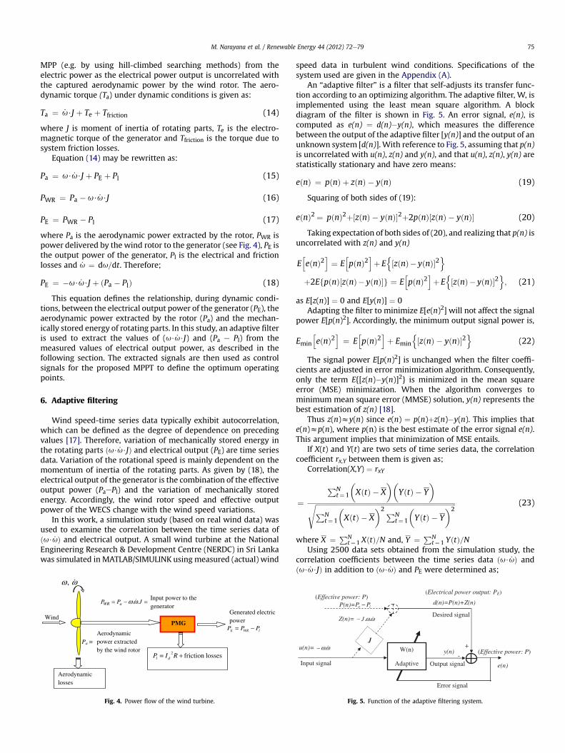
The signal ðu$ _uÞ is highly correlated with variation of mechan-ically stored energy ðu$ _u$JÞ and weakly correlated with electricaloutput power (PE). The signal of variation of mechanically storedenergy ðu$ _u$JÞ has zero mean. Therefore, an adaptive filter in noisecancellationmode canbeutilized tofilter the effective power (Pa�Pl)from the signal of electrical power (PE) output [19].

On the basis of this error, the adaptive filter changes its coeffi-cients in an attempt to reduce the error. The input signals to theadaptive filter are the electrical power output (PE) and ðu$ _uÞ.

Referring to Fig. 5;

uðnÞ ¼ �u$ _u, ZðnÞ ¼ �u$ _u$J and d(n) ¼ PE.

dðnÞ ¼ PðnÞ þ ZðnÞ

yðnÞ ¼XN�1

k¼0

WðkÞ$uðn� kÞ (24)

Where W ¼

2664

Wð0ÞWð1Þ

«WðN � 1Þ

3775

yðnÞ ¼ WTðn� 1Þ$uðnÞ (25)

eðnÞ ¼ dðnÞ � yðnÞ (26)

WðnÞ ¼ Wðn� 1Þ þ f ðeðnÞ;uðnÞ;mÞ (27)

0>dt

dω

Rotational speed (ω)

0<dt

dω

ωΔ−ΔPωΔ−

Δ− P

ωΔΔ− P

ωΔΔP

Eff

ectiv

e Po

wer

Fig. 7. Control criteria.

where f(e(n),u(n),m) is the weight update function and m is theadaptation step size.

A Least Mean Square (LMS) algorithm was used to estimate theweights of the filter [19,20]. In this study, an adaptive system witha length of 16 elements was used to identify the input controlsignals. The outputs of the adaptive filter are; ZðnÞ ¼ �u$ _u$J andP(n) ¼ Pa�Pl.

Performance of the adaptive filter when used with the NERDCwind turbine system is illustrated in Fig. 6 where the calculatedeffective power and variation of mechanically stored energy arecompared with the outputs of the adaptive system. Simulationresults show that Pa�Pl and ðu$ _u$JÞ signals can be extracted fromthe input signals PE andðu$ _uÞ with reasonable accuracy. Therefore,by using an adaptive filter, appropriate control signals to define theoptimum MPPs can be extracted from the measured wind turbinesystem outputs.

7. “Fuzzy Logic” optimal power point tracking controller

The power loss in the electric generator is proportional to thegenerated power. As the electrical output is combined with thevariation of mechanically stored energy in the rotating parts(u$ _u$J), power loss varies with the variation of mechanically storedenergy. As the power loss increases when u$ _u$J < 0 and decreaseswhenu$ _u$J > 0, the effective power curve varies with variation of

0

1

ωddP

-20 0 -10 10 20

Output,

UM UL

0 -0.03 -0.06 -0.09 0.03 0.06 0.09 0

RH RM RL NC UH 1

Fig. 8. Related fuzzy sets.

J . . ω ω ω d

dP - -

Wind Energy Conversion S y ste m

Output power potential

Wind s p ee d

Fuzzy logic controller

Adaptive digital filter

×

× ÷

P E P=P a -P l

Outputs

dt

d dt

d ω ω . ω ω . −

P

ω

ω J . . ω ω −

Fig. 9. The proposed generic control system.

M. Narayana et al. / Renewable Energy 44 (2012) 72e79 77

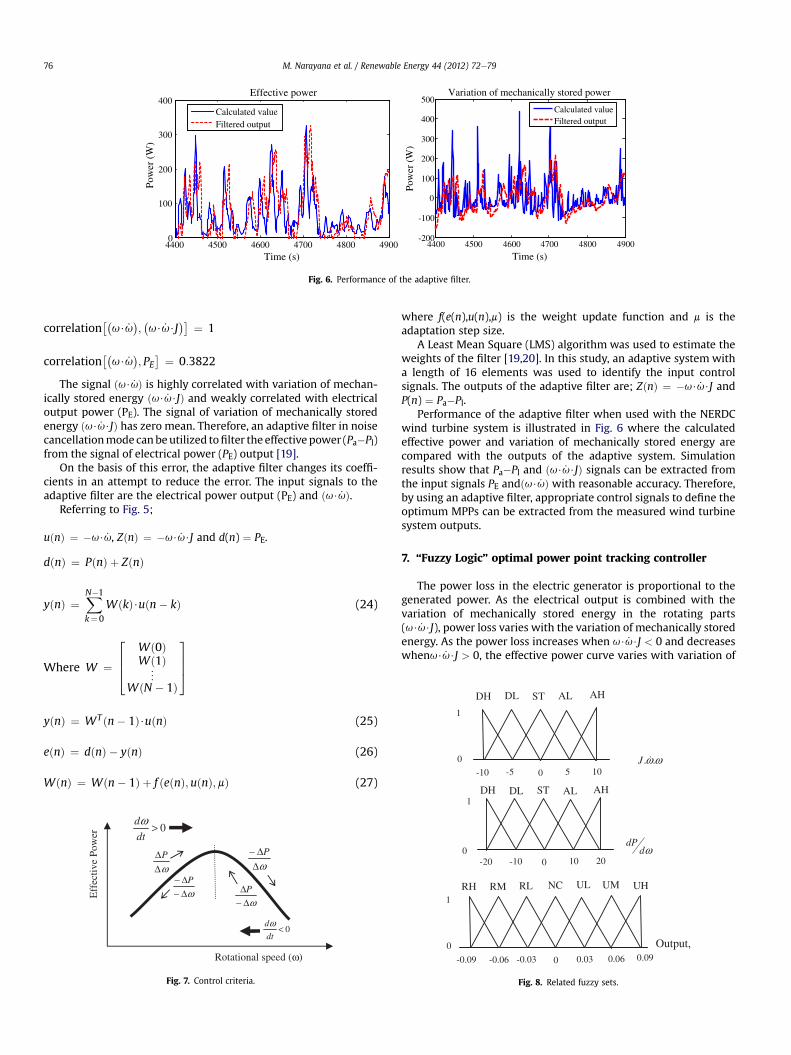
mechanically stored energy. The system needs to operate at themaximum point of the effective power curve to optimize energyharvesting. This is the optimum operating point of the combinedsystem of the wind rotor and the electric generator. Thehill-climbing control criterion (presented in Fig. 7) can be followedto track the optimum power points for any u$ _u$J. As the systemparameters cannot be evaluated, exact relations between inputsand outputs of the system cannot be enumerated. Therefore,a “Fuzzy Logic” controller is introduced to optimize the perfor-mance of the system by considering qualitative parameters offiltered signals from the system outputs. At optimum operatingpoint dP/du ¼ 0 (see Fig. 7). The rotational speed of the wind rotoris controlled by varying the electrical load on the system. The valueof dP/du indicates the deviation of actual operating point from theoptimum operating point and the value of u$ _u$J indicates status ofdynamics of the system. Therefore according to u$ _u$J and dP/du,the changing of wind rotor rotational speed step size can bemodified for quicker response time to achieve the optimum oper-ating point. Related “Fuzzy sets” and “Fuzzy rules” were developedby considering u$ _u$J and dP/du and are presented in Fig. 8 andAppendix (B) (where P ¼ Pa�Pl). The Centroid defuzzificationmethod was used to obtain the “Fuzzy set” outputs (Dd) [21]. Ablock diagram of the proposed Fuzzy Logic basedMPPTcontroller isshown in Fig. 9.

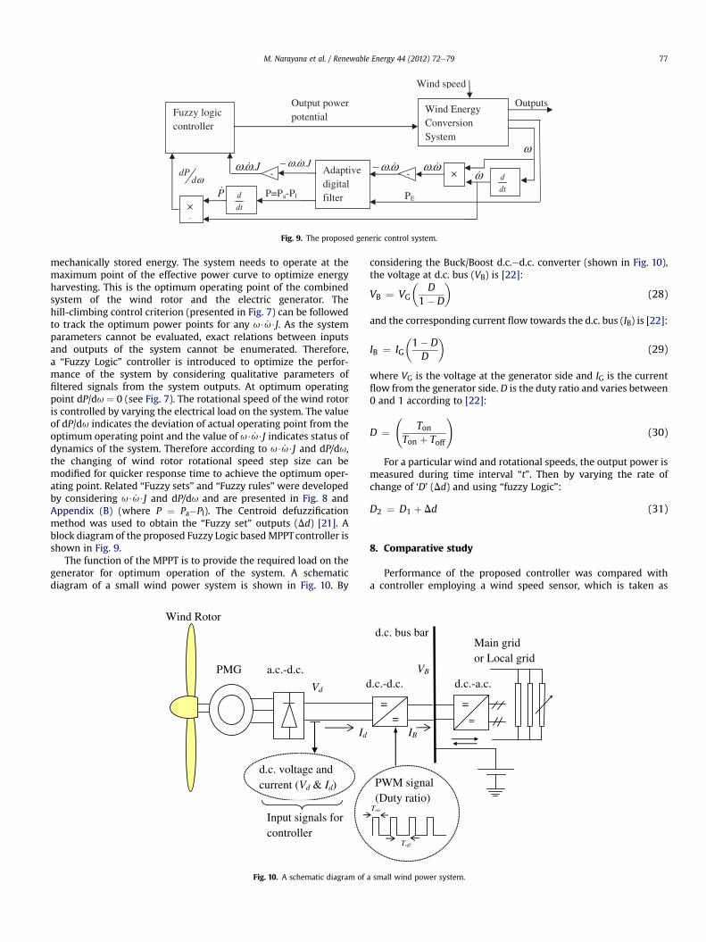
The function of the MPPT is to provide the required load on thegenerator for optimum operation of the system. A schematicdiagram of a small wind power system is shown in Fig. 10. By

Wind Rotor

PMG a.c.-d.c. d

Input signals for controller

d.c. voltage and current (Vd & Id)

Id

Vd

Fig. 10. A schematic diagram of a

considering the Buck/Boost d.c.ed.c. converter (shown in Fig. 10),the voltage at d.c. bus (VB) is [22]:

VB ¼ VG

�D

1� D

�(28)

and the corresponding current flow towards the d.c. bus (IB) is [22]:

IB ¼ IG

�1� DD

�(29)

where VG is the voltage at the generator side and IG is the currentflow from the generator side. D is the duty ratio and varies between0 and 1 according to [22]:

D ¼

TonTon þ Toff

!(30)

For a particular wind and rotational speeds, the output power ismeasured during time interval “t”. Then by varying the rate ofchange of ‘D’ (Dd) and using “fuzzy Logic”:

D2 ¼ D1 þ Dd (31)

8. Comparative study

Performance of the proposed controller was compared witha controller employing a wind speed sensor, which is taken as

Ton

Toff

Main grid or Local grid

d.c. bus bar

d.c.-a.c. .c.-d.c.

= =

PWM signal (Duty ratio)

VB

IB

=

small wind power system.

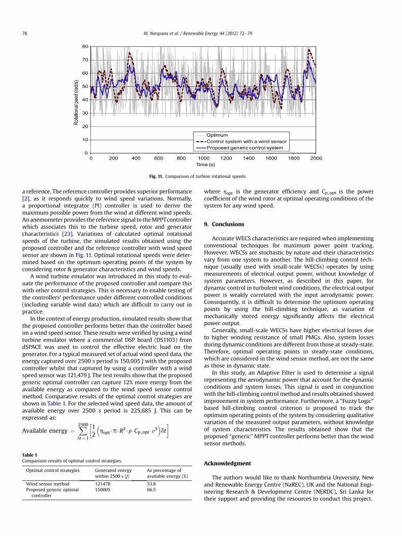
Fig. 11. Comparison of turbine rotational speeds.

M. Narayana et al. / Renewable Energy 44 (2012) 72e7978

a reference. The reference controller provides superior performance[2], as it responds quickly to wind speed variations. Normally,a proportional integrator (PI) controller is used to derive themaximum possible power from the wind at different wind speeds.An anemometer provides the reference signal to theMPPTcontrollerwhich associates this to the turbine speed, rotor and generatorcharacteristics [23]. Variations of calculated optimal rotationalspeeds of the turbine, the simulated results obtained using theproposed controller and the reference controller with wind speedsensor are shown in Fig. 11. Optimal rotational speeds were deter-mined based on the optimum operating points of the system byconsidering rotor & generator characteristics and wind speeds.

A wind turbine emulator was introduced in this study to eval-uate the performance of the proposed controller and compare thiswith other control strategies. This is necessary to enable testing ofthe controllers’ performance under different controlled conditions(including variable wind data) which are difficult to carry out inpractice.

In the context of energy production, simulated results show thatthe proposed controller performs better than the controller basedon awind speed sensor. These results were verified by using awindturbine emulator where a commercial DSP board (DS1103) fromdSPACE was used to control the effective electric load on thegenerator. For a typical measured set of actual wind speed data, theenergy captured over 2500 s period is 150,005 J with the proposedcontroller whilst that captured by using a controller with a windspeed sensor was 121,479 J. The test results show that the proposedgeneric optimal controller can capture 12% more energy from theavailable energy as compared to the wind speed sensor controlmethod. Comparative results of the optimal control strategies areshown in Table 1. For the selected wind speed data, the amount ofavailable energy over 2500 s period is 225,685 J. This can beexpressed as:

Available energy ¼X2500dt¼1

12

hopt$p$R

2$r$Cp opt$v3�dt�

Table 1Comparison results of optimal control strategies.

Optimal control strategies Generated energywithin 2500 s (J)

As percentage ofavailable energy (%)

Wind sensor method 121478 53.8Proposed generic optimal

controller150005 66.5

where hopt is the generator efficiency and Cp_opt is the powercoefficient of the wind rotor at optimal operating conditions of thesystem for any wind speed.

9. Conclusions

AccurateWECS characteristics are required when implementingconventional techniques for maximum power point tracking.However, WECSs are stochastic by nature and their characteristicsvary from one system to another. The hill-climbing control tech-nique (usually used with small-scale WECSs) operates by usingmeasurements of electrical output power, without knowledge ofsystem parameters. However, as described in this paper, fordynamic control in turbulent wind conditions, the electrical outputpower is weakly correlated with the input aerodynamic power.Consequently, it is difficult to determine the optimum operatingpoints by using the hill-climbing technique, as variation ofmechanically stored energy significantly affects the electricalpower output.

Generally, small-scale WECSs have higher electrical losses dueto higher winding resistance of small PMGs. Also, system lossesduring dynamic conditions are different from those at steady-state.Therefore, optimal operating points in steady-state conditions,which are considered in the wind sensor method, are not the sameas those in dynamic state.

In this study, an Adaptive Filter is used to determine a signalrepresenting the aerodynamic power that account for the dynamicconditions and system losses. This signal is used in conjunctionwith the hill-climbing control method and results obtained showedimprovement in system performance. Furthermore, a “Fuzzy Logic”based hill-climbing control criterion is proposed to track theoptimum operating points of the system by considering qualitativevariation of the measured output parameters, without knowledgeof system characteristics. The results obtained show that theproposed “generic”MPPT controller performs better than the windsensor methods.

Acknowledgment

The authors would like to thank Northumbria University, Newand Renewable Energy Centre (NaREC), UK and the National Engi-neering Research & Development Centre (NERDC), Sri Lanka fortheir support and providing the resources to conduct this project.

M. Narayana et al. / Renewable Energy 44 (2012) 72e79 79

Appendices

a. Specifications of the NERDC small wind turbine.

Rated capacity 200 WRadius of the wind rotor 1.105 mNumber of blades 2Moment of inertia of rotating parts (J) 9.77 kg m2

Generator Permanent magnet (34)No. of pole pairs 6Stator phase resistance 1.25 UInductances [Ld, Lq] [0.003075H, 0.003075H]Flux linkage by magnets 0.098 V.s

Frictional factor 9.444 � 10e15 N.m.s

b. Fuzzy rules.

If u$ _u$J is and dP=du is Then Dd is

1. DH DH NC2. DL DH UM3. ST DH NC4. AL DH UM5. AH DH UH6. DH DL UM7. DL DL NC8. ST DL NC9. AL DL UL10. AH DL UM11. DH ST NC12. DL ST NC13. ST ST NC14. AL ST NC15. AH ST NC16. DH AL RM17. DL AL RL18. ST AL NC19. AL AL NC20. AH AL RM21. DH AH RH22. DL AH RM23. ST AH NC24. AL AH RM25. AH AH NC

References

[1] Muljadi E, Pierce K, Migliore P. Soft-control control for variable-speed stall-regulated wind turbines. Wind Engineering 2000;85:277e91.

[2] Jamal AB, Dinavahi V, Knight A. A review of power converter topologies forwind turbines. Renewable Energy 2007;32:2369e85.

[3] Belakehal S, Benalla H, Bentounsi A. Power maximization control of smallwind system using permanent magnet synchronous generator. Revue desEnergies Renouvelables 2009;12:307e19.

[4] Gourieres DL. Wind power plants theory and design. Oxford: Pergamon Press;1982.

[5] Burton T, Sharpe D, Jenkins N, Bossanyi E. Wind energy handbook. John Wiley& Sons, Ltd; 2001.

[6] Muljadi E, Butterfield CP, Wan YH. Axial flux, modular, permanent-magnetgenerator with a toroidal winding for wind turbine applications. IEEEindustry applications conference St. Louis, Mo; 1998.

[7] Khan MA, Pillay P. Design of a PM wind generator, optimised for energycapture over a wide operating range. IEEE international conference on electricmachines and drives; 2005. pp. 1501e1506.

[8] Leonhard W. Controls of electrical drives. 3rd ed. Berlin Heidelberg New York:Springer; 2001.

[9] Munteanu L, Bratcu AL, Cutululis NA, Ceanga E. Optimal control of wind energysystem: towards a global approach. Springer-Verlag London Limited; 2008.

[10] Yin M, Li G, Zhou M, Zhao C. Modelling of the wind turbine with a permanentmagnet synchronous generator for integration. Power engineering societygeneral meeting IEEE; 2007. pp. 1e6.

[11] Grenier D, Dessaint LA, Akhrif O, Bonnassieux Y, Le Pioufle B. Experimentalnonlinear torque control of a permanent-magnet synchronous motor usingsaliency. Industrial Electronics, IEEE Transactions 1997;44:680e7.

[12] Arifujjaman Md, Iqbal MT, Quaice JE. Energy capture by a small wind-energyconversion system. Applied Energy 2008;85:41e51.

[13] Morimoto S, Nakayama H, Sanada M, Takeda Y. Sensorless output maximi-zation control for variable-speed wind generation system using IPMSG. IEEETransaction on Industry Applications Jan/Feb 2005;41:60e7.

[14] Tan K, Islam S. Optimum control strategies in energy conversion of PMSGwind turbine system without mechanical sensors. IEEE Transaction on EnergyConversion June 2004;19:392e9.

[15] Tanaka T, Toumiya T. Output control by hill-climbing method for a small scalewind power generation system. Renewable Energy 1997;12:387e400.

[16] Koutroulis E, Kalaitzakis K. Design of a maximum power tracking system forwind-energy-conversion application. IEEE Transaction on Industrial Elec-tronics April 2006;53:486e94.

[17] Riahy GH, Abedi M. Short term wind speed forecasting for wind turbine applica-tions using linear prediction method. Renewable Energy 2008;33:35e41.

[18] Widrow B, Glover Jr JR, McCool JM, Kaunitz J, Williams CS, Hearn RH, et al.Adaptive noise cancelling: principles and applications. Proceedings of theIEEE, vol. 63, pp. 1692e1716; 1975.

[19] Goodwin GC, Sin KS. Adaptive filtering prediction and control. EnglewoodCliffs: Prentice Hall, Inc; 1984.

[20] Haykin S. Adaptive filter theory. Englewood Cliffs, NJ: Prentice Hall; 1986.[21] Ross TJ. Fuzzy logic with engineering applications. McGraw-Hill. Inc.; 1995.[22] Mohan N, Underland TM, Robbins WP. Power electronics converters, appli-

cation and design. 3rd ed. John Wiley and Sons; 2003.[23] Wang Q, Chang L. An intelligent maximum power extraction algorithm for

Inverter-based variable speed wind turbine systems. IEEE Transaction onPower Electronics September 2004;19:1242e9.