Embed Size (px)
Citation preview
geneXtendeR
Bohdan B. Khomtchouk
April 30, 2018
Introduction
This vignette describes geneXtendeR (Khomtchouk et al. 2016), an R/Bioconductorpackage for optimized annotation of genomic features (primarily peaks calledfrom a ChIP-seq experiment, but any coverage island regions would work) withthe nearest gene. “Extending" refers to performing gene-feature overlaps af-ter adding to the gene-span a user-specified region upstream of the start ofthe gene model and a fixed (500 bp) region downstream of the gene, resultingin assigning to a gene the features that do not physically overlap with it butare sufficiently close. Extending is an automated iterative procedure in geneX
tendeR, allowing the user to repeatedly align peaks to multiple gene transferformat (GTF) files to assess what global gene-spans optimize the genomewidealignment of peaks with their closest genes. This facilitates the process of de-ciphering which differentially enriched peaks are dysregulating which specificgenes. This, in turn, aids experimental follow-up and validation in designingprimers for a set of prospective genes during qPCR (Barbier et al. 2016).
Rationale
With an abundance of Bioconductor software currently available for peak an-notation to nearby features (e.g., ChIPpeakAnno (Zhu et al. 2010)) as well asthe existence of various command line tools (e.g., BEDTools closest function(Quinlan and Hall, 2010), HOMER (Heinz et al. 2010)), what makes geneXten
deR different? The simple answer is: geneXtendeR is designed for assessing thevariability of peak overlap with cis-regulatory elements and proximal-promoterregions. It is well-known that peak coordinates (peak start position, peak endposition) exhibit a considerable degree of variance depending on the peak callerused (e.g., SICER (Zang et al. 2009), MACS2 (Zhang et al. 2008), etc.),
both in terms of length distribution of peaks as well as the total number ofpeaks called, even when run at identical default parameter values (Koohy etal. 2014; Thomas et al. 2017). Tuning algorithm-specific parameters produceseven greater variance amongst peak callers, thereby complicating the issue fur-ther. This variance becomes a factor when annotating peak lists genome-widewith their nearest genes as, depending on the peak caller, peaks can be eithershifted in genomic position (towards 5’ or 3’ end) or be of different lengths.As such, geneXtendeR represents a first step towards tailoring (or customizing)the functional annotation of a ChIP-seq peak dataset according to the detailsof the peak coordinates (chromosome number, peak start position, peak endposition).
The primary focus of geneXtendeR is to optimize the process of functionalannotation of a ChIP-seq peak list whereby instead of just annotating peakswith their nearest genomic features (as statically defined by a given genomebuild’s coordinates), geneXtendeR investigates how peaks dynamically align tovarious user-specified gene extensions (e.g., 500 bp upstream extensions, 2000bp upstream extensions, etc. for all genes in the genome). This shows wherepeaks localize across the genome with respect to their nearest gene, as well aswhat gene ontologies (BP, CC, and MF) are impacted at these various extensionlevels. This, in turn, informs the user what gene extensions ideally capture theGO terms involved in the biology of their experiment. For example, if a user’sstudy is investigating the role of epigenetic enzymes in alcohol addiction anddependence, then functionally annotating a peak list using gene extensions thatmaximize the number of brain-related ontologies (for both BP, CC, and MFcategories) makes sense.
With regards to histone modification ChIP-seq analysis, geneXtendeR computesoptimal gene extensions tailored to the broadness of the specific epigenetic mark(e.g., H3K9me1, H3K27me3), as determined by a user-supplied ChIP-seq peakinput file. To accomplish this level of custom-tailored data analysis, geneXtendeR first optimally extends the boundaries of every gene in a genome by somegenomic distance (in DNA base pairs) for the purpose of flexibly incorporatingcis-regulatory elements, such as promoter regions, as well as downstream ele-ments that are important to the function of the gene relative to an epigenetichistone modification ChIP-seq dataset. This action effectively transforms genesinto “gene-spheres", a new term that we coin to emphasize the 3D-nature ofheterochromatin. A gene-sphere is composed of cis-regulatory elements (e.g.,proximal promoters +/- ≈ 3 kb from TSS), distal regulatory elements (e.g.,enhancers), transcription start/end sites (TSS/TES), exons, introns, and down-stream elements of a gene. As such, geneXtendeR maximizes the signal-to-noiseratio of locating genes closest to and directly under peaks. By performing acomputational expansion of this nature, ChIP-seq reads that would initially notmap strictly to a specific gene can now be optimally mapped to the regula-
2
tory regions of the gene, thereby implicating the gene as a potential candidate,and thereby making the ChIP-seq analysis more successful. Such an approachbecomes particularly important when working with epigenetic histone modifica-tions that have inherently broad peaks with a diffuse range of signal enrichment(e.g., H3K9me1, H3K27me3).
Quick start
First, install the geneXtendeR package via:
> ## try http:// if https:// URLs are not supported
> source("https://bioconductor.org/biocLite.R")
> biocLite("geneXtendeR")
> library(geneXtendeR)
This automatically loads the rtracklayer R package, which contains the read
GFF() command used to retrieve GTF files of any model organism. As such,load in a GTF file into your R environment, e.g.:
> rat <- readGFF("ftp://ftp.ensembl.org/pub/release-84/gtf/
+ rattus_norvegicus/Rattus_norvegicus.Rnor_6.0.84.chr.gtf.gz")
URLs may be obtained as direct links from: http://useast.ensembl.org/info/data/ftp/index.html. Click on the “GTF" link under the “Gene sets" columnfor a particular species and then right-click (or command-click on Mac OS X) thename of the file containing the species name/version number and file extensionchr.gtf.gz (e.g., Homo_sapiens.GRCh38.84.chr.gtf.gz, Mus_musculus.GRCm38.84.chr.gtf.gz,etc.), and copy the link address. Then, paste the link address into the read
GFF() as shown above. This will create an R dataframe object containing therespective GTF file.
Next, the user must input their peak data from a peak caller (e.g., SICER,MACS2, etc.). The peak data must contain only three tab-delimited columns(chromosome number, peak start, and peak end) and a header containing:“chr", “start", and “end". See ?samplepeaksinput for an example. Once thepeak input data (e.g., “somepeaksfile.txt") has been assembled properly (i.e.,to contain only the three tab-delimited columns and header above), it must beproperly formatted prior to the execution of downstream analyses.
First, the user must set their working directory to point to the location of theirpeak data file. Then type the following command:
3
1Similarly, userscan transform theirpeaks file into a fileof merged peaks(see peaksMerge())and use the resul-tant “peaks.txt"file instead for thesubsequent analysis.2This peaks datasetcomes from a ChIP-seq investigation ofbrain tissue (pre-frontal cortex) in al-cohol addiction anddependence (Bar-bier et al. 2016),see References sec-tion for details.
> peaksInput("somepeaksfile.txt")
This command properly formats the user’s peaks file in preparation for sub-sequent analyses, producing a resultant “peaks.txt" file in the user’s workingdirectory1.
To see how the above command works using a built-in example, the geneXten
deR package provides a peak input dataset2 called “somepeaksfile.txt", whichcan be loaded into memory like this:
> fpath <- system.file("extdata", "somepeaksfile.txt", package="geneXtendeR")
> peaksInput(fpath)
This creates a properly formatted (i.e., properly sorted) “peaks.txt" file in theuser’s working directory.
Now, we may use the R object that we created with readGFF() earlier to createa bar chart visualization showing the number of peaks that are sitting directly ontop of genes across a series of upstream extensions (of each gene in a genome):
4
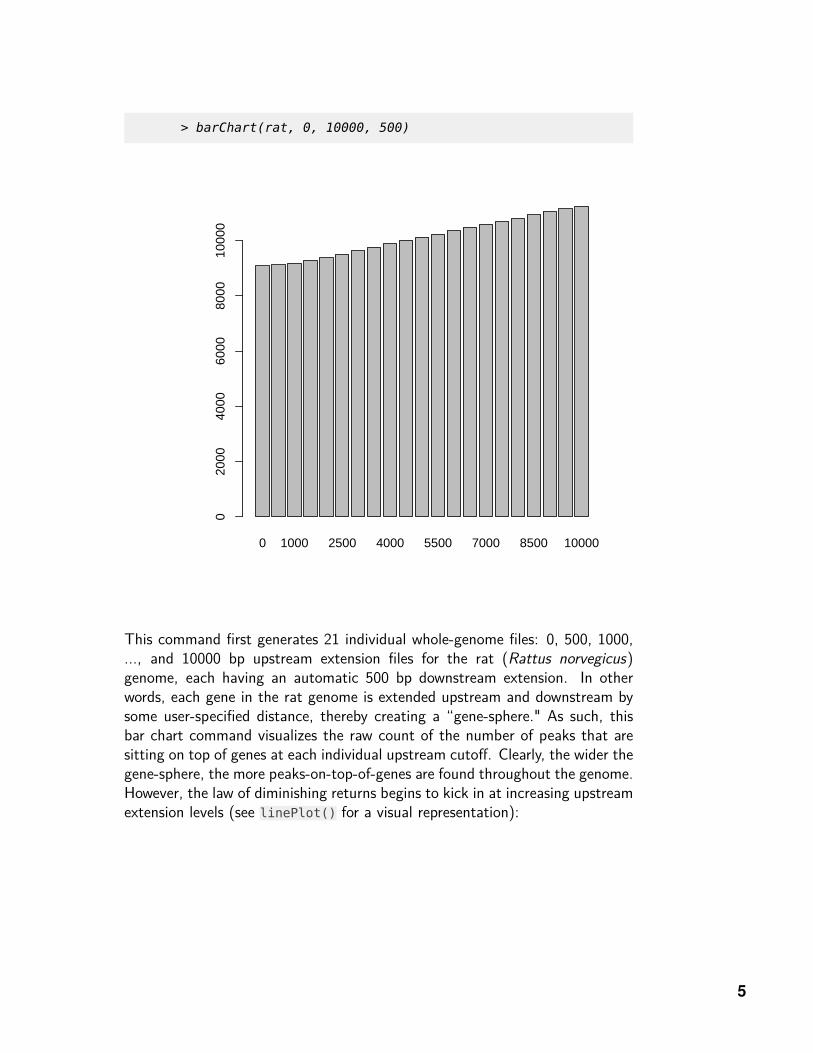
> barChart(rat, 0, 10000, 500)
0 1000 2500 4000 5500 7000 8500 10000
020
0040
0060
0080
0010
000
This command first generates 21 individual whole-genome files: 0, 500, 1000,..., and 10000 bp upstream extension files for the rat (Rattus norvegicus)genome, each having an automatic 500 bp downstream extension. In otherwords, each gene in the rat genome is extended upstream and downstream bysome user-specified distance, thereby creating a “gene-sphere." As such, thisbar chart command visualizes the raw count of the number of peaks that aresitting on top of genes at each individual upstream cutoff. Clearly, the wider thegene-sphere, the more peaks-on-top-of-genes are found throughout the genome.However, the law of diminishing returns begins to kick in at increasing upstreamextension levels (see linePlot() for a visual representation):
5
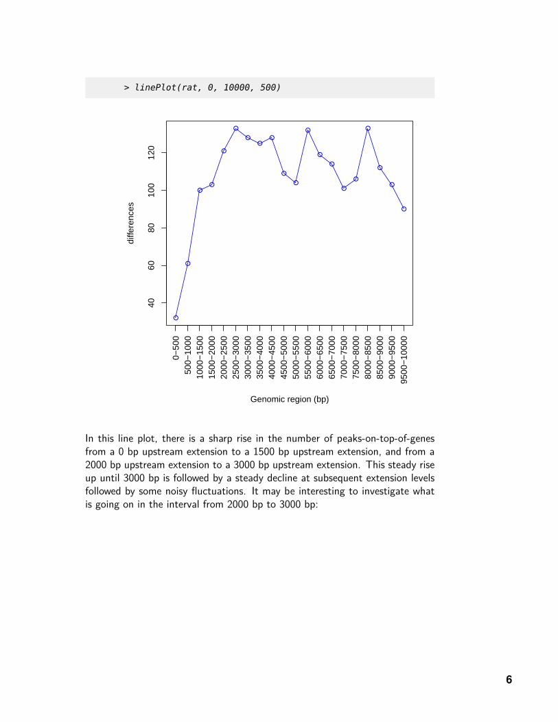
> linePlot(rat, 0, 10000, 500)
●
●
●●
●
●
●●
●
●
●
●
●
●
●
●
●
●
●
●
4060
8010
012
0
diffe
renc
es
0−50
050
0−10
0010
00−
1500
1500
−20
0020
00−
2500
2500
−30
0030
00−
3500
3500
−40
0040
00−
4500
4500
−50
0050
00−
5500
5500
−60
0060
00−
6500
6500
−70
0070
00−
7500
7500
−80
0080
00−
8500
8500
−90
0090
00−
9500
9500
−10
000
Genomic region (bp)
In this line plot, there is a sharp rise in the number of peaks-on-top-of-genesfrom a 0 bp upstream extension to a 1500 bp upstream extension, and from a2000 bp upstream extension to a 3000 bp upstream extension. This steady riseup until 3000 bp is followed by a steady decline at subsequent extension levelsfollowed by some noisy fluctuations. It may be interesting to investigate whatis going on in the interval from 2000 bp to 3000 bp:
6
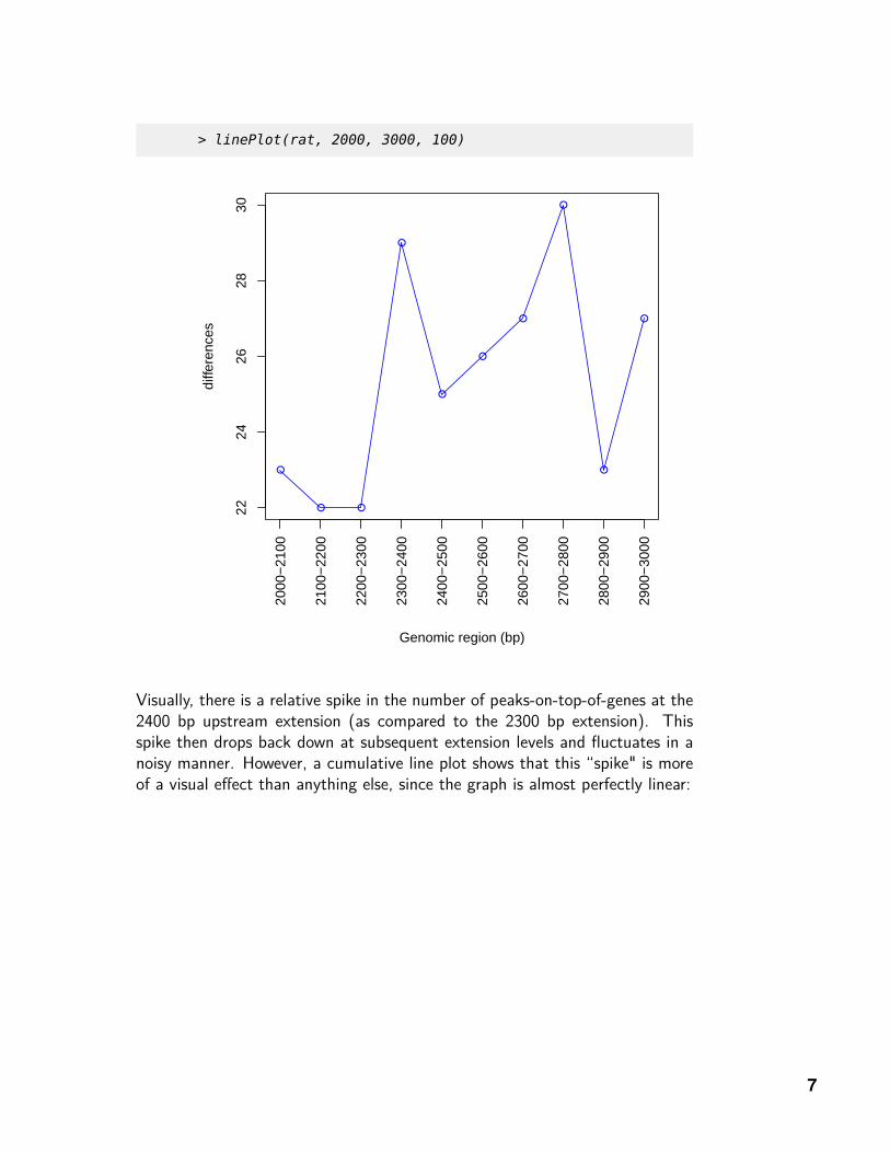
> linePlot(rat, 2000, 3000, 100)
●
● ●
●
●
●
●
●
●
●
2224
2628
30
diffe
renc
es
2000
−21
00
2100
−22
00
2200
−23
00
2300
−24
00
2400
−25
00
2500
−26
00
2600
−27
00
2700
−28
00
2800
−29
00
2900
−30
00Genomic region (bp)
Visually, there is a relative spike in the number of peaks-on-top-of-genes at the2400 bp upstream extension (as compared to the 2300 bp extension). Thisspike then drops back down at subsequent extension levels and fluctuates in anoisy manner. However, a cumulative line plot shows that this “spike" is moreof a visual effect than anything else, since the graph is almost perfectly linear:
7
3Note that statis-tical significance isset apriori by theuser at the peakcalling stage (priorto geneXtendeR) togive the user thefreedom to choosehow to filter outpeak coordinatesthat only pass spe-cific p-value andFDR cutoffs froma peak caller. Peakcaller output (e.g.,from SICER) givesboth p-value andFDR measures foreach peak, therebymaking it easy toextract only thepeak coordinatesthat pass a specificset of statisticalcutoff criteria.
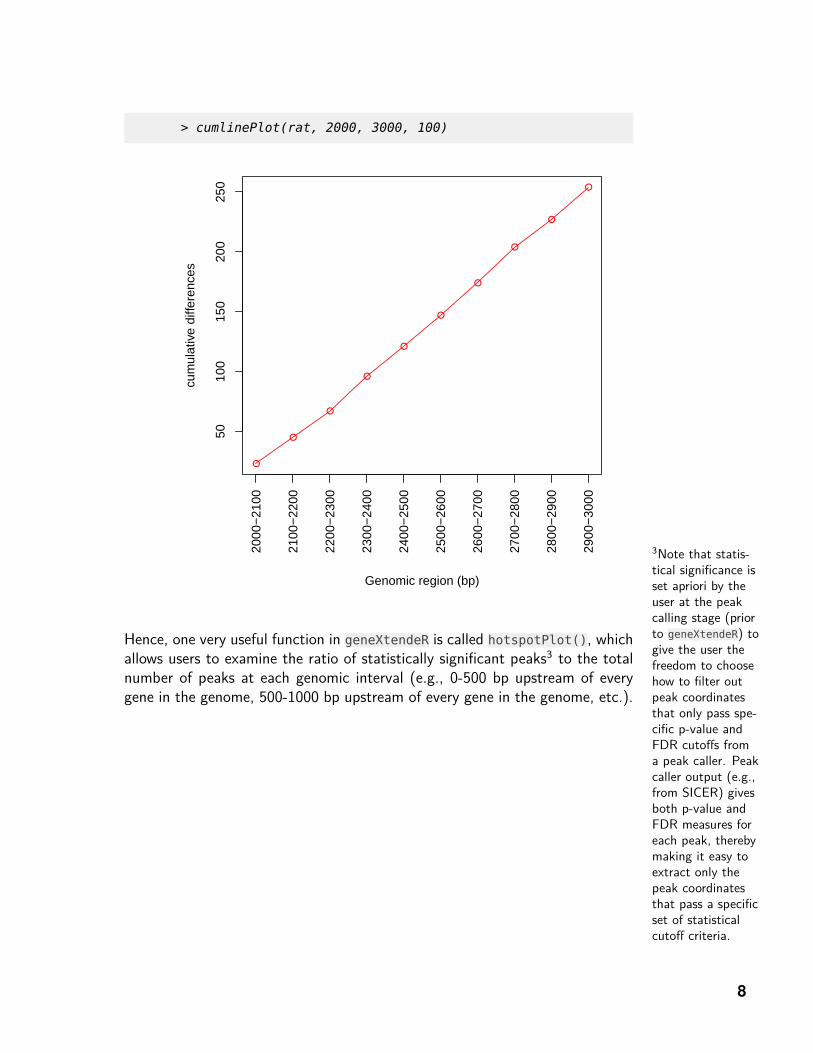
> cumlinePlot(rat, 2000, 3000, 100)
●
●
●
●
●
●
●
●
●
●
5010
015
020
025
0
cum
ulat
ive
diffe
renc
es
2000
−21
00
2100
−22
00
2200
−23
00
2300
−24
00
2400
−25
00
2500
−26
00
2600
−27
00
2700
−28
00
2800
−29
00
2900
−30
00Genomic region (bp)
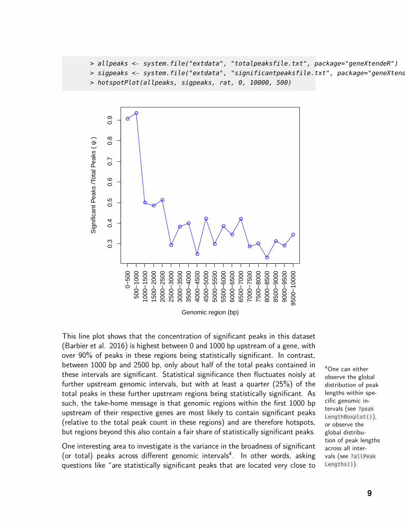
Hence, one very useful function in geneXtendeR is called hotspotPlot(), whichallows users to examine the ratio of statistically significant peaks3 to the totalnumber of peaks at each genomic interval (e.g., 0-500 bp upstream of everygene in the genome, 500-1000 bp upstream of every gene in the genome, etc.).
8
4One can eitherobserve the globaldistribution of peaklengths within spe-cific genomic in-tervals (see ?peak
LengthBoxplot()),or observe theglobal distribu-tion of peak lengthsacross all inter-vals (see ?allPeak
Lengths()).
> allpeaks <- system.file("extdata", "totalpeaksfile.txt", package="geneXtendeR")
> sigpeaks <- system.file("extdata", "significantpeaksfile.txt", package="geneXtendeR")
> hotspotPlot(allpeaks, sigpeaks, rat, 0, 10000, 500)
●
●
●●
●
●
●●
●
●
●
●
●
●
●●
●
●●
●
0.3
0.4
0.5
0.6
0.7
0.8
0.9
Sig
nific
ant P
eaks
/Tot
al P
eaks
( ψ
)
0−50
050
0−10
0010
00−
1500
1500
−20
0020
00−
2500
2500
−30
0030
00−
3500
3500
−40
0040
00−
4500
4500
−50
0050
00−
5500
5500
−60
0060
00−
6500
6500
−70
0070
00−
7500
7500
−80
0080
00−
8500
8500
−90
0090
00−
9500
9500
−10
000
Genomic region (bp)
This line plot shows that the concentration of significant peaks in this dataset(Barbier et al. 2016) is highest between 0 and 1000 bp upstream of a gene, withover 90% of peaks in these regions being statistically significant. In contrast,between 1000 bp and 2500 bp, only about half of the total peaks contained inthese intervals are significant. Statistical significance then fluctuates noisly atfurther upstream genomic intervals, but with at least a quarter (25%) of thetotal peaks in these further upstream regions being statistically significant. Assuch, the take-home message is that genomic regions within the first 1000 bpupstream of their respective genes are most likely to contain significant peaks(relative to the total peak count in these regions) and are therefore hotspots,but regions beyond this also contain a fair share of statistically significant peaks.
One interesting area to investigate is the variance in the broadness of significant(or total) peaks across different genomic intervals4. In other words, askingquestions like “are statistically significant peaks that are located very close to
9
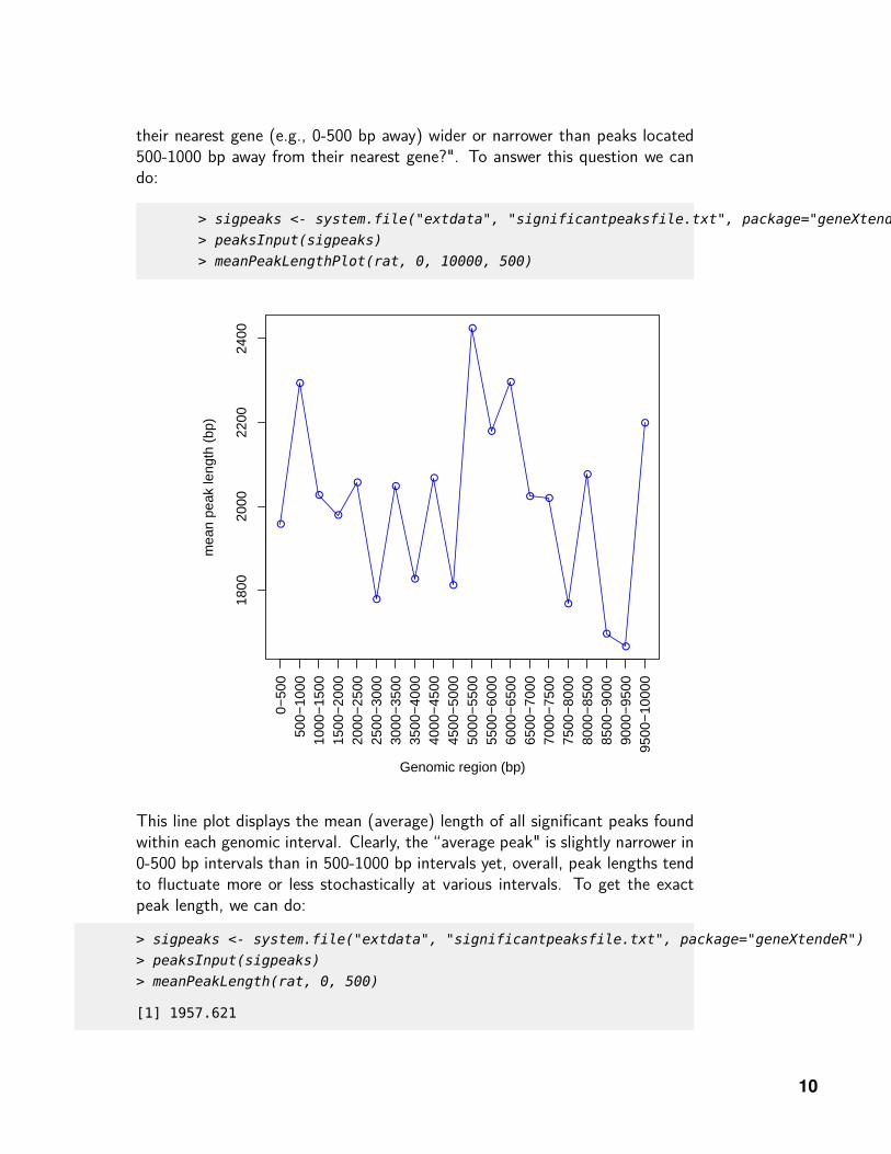
their nearest gene (e.g., 0-500 bp away) wider or narrower than peaks located500-1000 bp away from their nearest gene?". To answer this question we cando:
> sigpeaks <- system.file("extdata", "significantpeaksfile.txt", package="geneXtendeR")
> peaksInput(sigpeaks)
> meanPeakLengthPlot(rat, 0, 10000, 500)
●
●
●
●
●
●
●
●
●
●
●
●
●
● ●
●
●
●
●
●
1800
2000
2200
2400
mea
n pe
ak le
ngth
(bp
)
0−50
050
0−10
0010
00−
1500
1500
−20
0020
00−
2500
2500
−30
0030
00−
3500
3500
−40
0040
00−
4500
4500
−50
0050
00−
5500
5500
−60
0060
00−
6500
6500
−70
0070
00−
7500
7500
−80
0080
00−
8500
8500
−90
0090
00−
9500
9500
−10
000
Genomic region (bp)
This line plot displays the mean (average) length of all significant peaks foundwithin each genomic interval. Clearly, the “average peak" is slightly narrower in0-500 bp intervals than in 500-1000 bp intervals yet, overall, peak lengths tendto fluctuate more or less stochastically at various intervals. To get the exactpeak length, we can do:
> sigpeaks <- system.file("extdata", "significantpeaksfile.txt", package="geneXtendeR")
> peaksInput(sigpeaks)
> meanPeakLength(rat, 0, 500)
[1] 1957.621
10
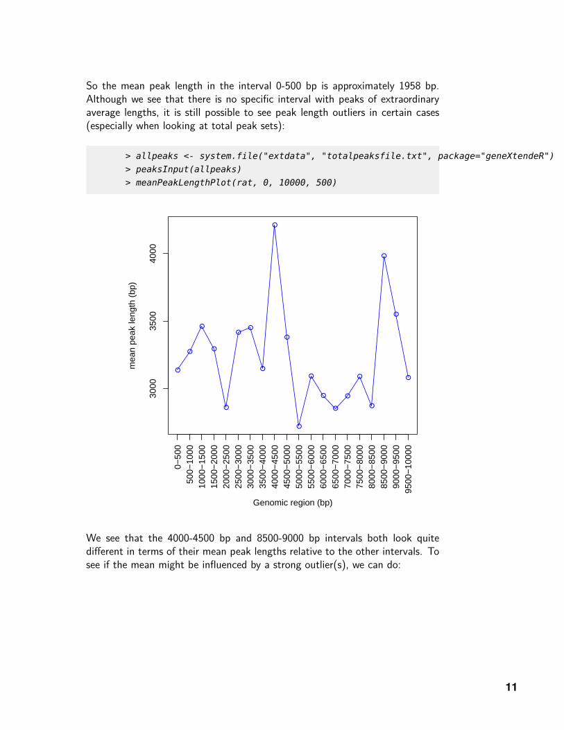
So the mean peak length in the interval 0-500 bp is approximately 1958 bp.Although we see that there is no specific interval with peaks of extraordinaryaverage lengths, it is still possible to see peak length outliers in certain cases(especially when looking at total peak sets):
> allpeaks <- system.file("extdata", "totalpeaksfile.txt", package="geneXtendeR")
> peaksInput(allpeaks)
> meanPeakLengthPlot(rat, 0, 10000, 500)
●
●
●
●
●
●●
●
●
●
●
●
●
●
●
●
●
●
●
●
3000
3500
4000
mea
n pe
ak le
ngth
(bp
)
0−50
050
0−10
0010
00−
1500
1500
−20
0020
00−
2500
2500
−30
0030
00−
3500
3500
−40
0040
00−
4500
4500
−50
0050
00−
5500
5500
−60
0060
00−
6500
6500
−70
0070
00−
7500
7500
−80
0080
00−
8500
8500
−90
0090
00−
9500
9500
−10
000
Genomic region (bp)
We see that the 4000-4500 bp and 8500-9000 bp intervals both look quitedifferent in terms of their mean peak lengths relative to the other intervals. Tosee if the mean might be influenced by a strong outlier(s), we can do:
11
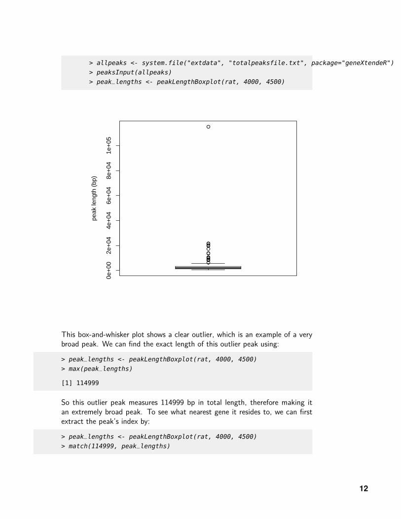
> allpeaks <- system.file("extdata", "totalpeaksfile.txt", package="geneXtendeR")
> peaksInput(allpeaks)
> peak_lengths <- peakLengthBoxplot(rat, 4000, 4500)
●●●
●
●
●
●
●
●●
●
●
●
●
●
0e+
002e
+04
4e+
046e
+04
8e+
041e
+05
peak
leng
th (
bp)
This box-and-whisker plot shows a clear outlier, which is an example of a verybroad peak. We can find the exact length of this outlier peak using:
> peak_lengths <- peakLengthBoxplot(rat, 4000, 4500)
> max(peak_lengths)
[1] 114999
So this outlier peak measures 114999 bp in total length, therefore making itan extremely broad peak. To see what nearest gene it resides to, we can firstextract the peak’s index by:
> peak_lengths <- peakLengthBoxplot(rat, 4000, 4500)
> match(114999, peak_lengths)
12
5This peak maynot be statisticallysignificant, buthow could it be ifit’s so huge? Insituations like this,it may be a goodidea to check whatis known about thegene already: http://panthertest2.usc.edu/genes/gene.do?acc=RAT%7CEnsembl=ENSRNOG00000028578%7CUniProtKB=A0A0G2K0W2.Clearly, not much isknown yet.
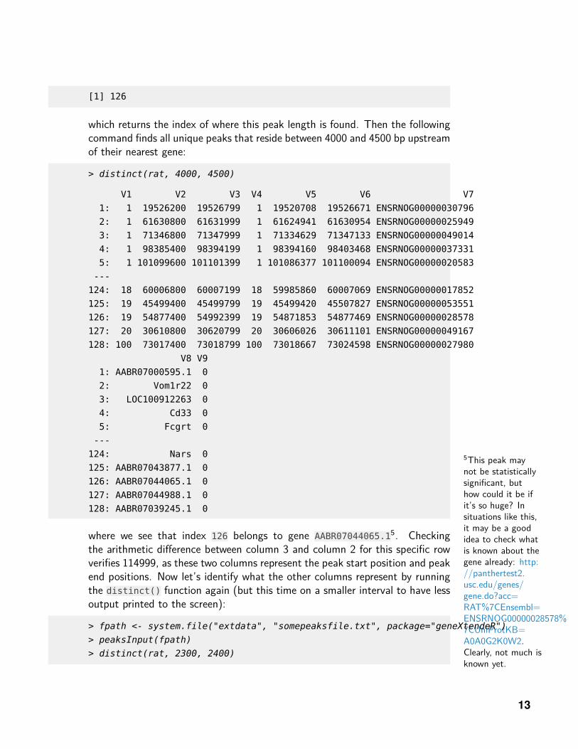
[1] 126
which returns the index of where this peak length is found. Then the followingcommand finds all unique peaks that reside between 4000 and 4500 bp upstreamof their nearest gene:
> distinct(rat, 4000, 4500)
V1 V2 V3 V4 V5 V6 V7
1: 1 19526200 19526799 1 19520708 19526671 ENSRNOG00000030796
2: 1 61630800 61631999 1 61624941 61630954 ENSRNOG00000025949
3: 1 71346800 71347999 1 71334629 71347133 ENSRNOG00000049014
4: 1 98385400 98394199 1 98394160 98403468 ENSRNOG00000037331
5: 1 101099600 101101399 1 101086377 101100094 ENSRNOG00000020583
---
124: 18 60006800 60007199 18 59985860 60007069 ENSRNOG00000017852
125: 19 45499400 45499799 19 45499420 45507827 ENSRNOG00000053551
126: 19 54877400 54992399 19 54871853 54877469 ENSRNOG00000028578
127: 20 30610800 30620799 20 30606026 30611101 ENSRNOG00000049167
128: 100 73017400 73018799 100 73018667 73024598 ENSRNOG00000027980
V8 V9
1: AABR07000595.1 0
2: Vom1r22 0
3: LOC100912263 0
4: Cd33 0
5: Fcgrt 0
---
124: Nars 0
125: AABR07043877.1 0
126: AABR07044065.1 0
127: AABR07044988.1 0
128: AABR07039245.1 0
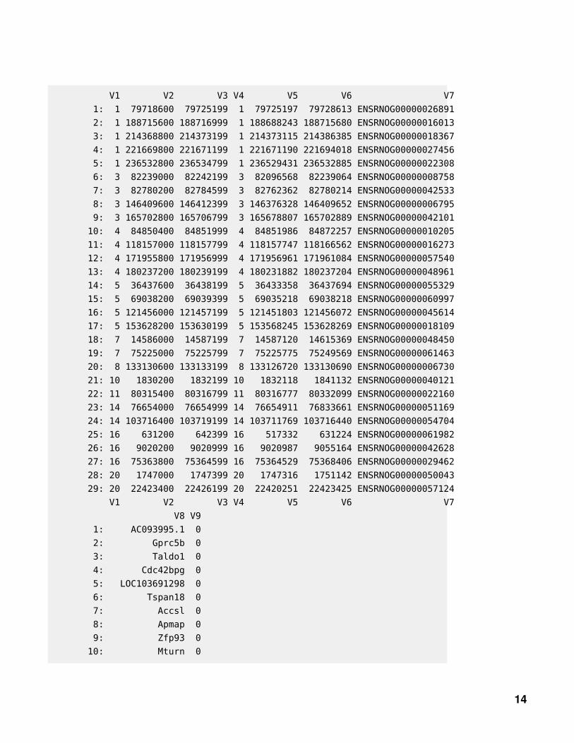
where we see that index 126 belongs to gene AABR07044065.15. Checkingthe arithmetic difference between column 3 and column 2 for this specific rowverifies 114999, as these two columns represent the peak start position and peakend positions. Now let’s identify what the other columns represent by runningthe distinct() function again (but this time on a smaller interval to have lessoutput printed to the screen):
> fpath <- system.file("extdata", "somepeaksfile.txt", package="geneXtendeR")
> peaksInput(fpath)
> distinct(rat, 2300, 2400)
13
V1 V2 V3 V4 V5 V6 V7
1: 1 79718600 79725199 1 79725197 79728613 ENSRNOG00000026891
2: 1 188715600 188716999 1 188688243 188715680 ENSRNOG00000016013
3: 1 214368800 214373199 1 214373115 214386385 ENSRNOG00000018367
4: 1 221669800 221671199 1 221671190 221694018 ENSRNOG00000027456
5: 1 236532800 236534799 1 236529431 236532885 ENSRNOG00000022308
6: 3 82239000 82242199 3 82096568 82239064 ENSRNOG00000008758
7: 3 82780200 82784599 3 82762362 82780214 ENSRNOG00000042533
8: 3 146409600 146412399 3 146376328 146409652 ENSRNOG00000006795
9: 3 165702800 165706799 3 165678807 165702889 ENSRNOG00000042101
10: 4 84850400 84851999 4 84851986 84872257 ENSRNOG00000010205
11: 4 118157000 118157799 4 118157747 118166562 ENSRNOG00000016273
12: 4 171955800 171956999 4 171956961 171961084 ENSRNOG00000057540
13: 4 180237200 180239199 4 180231882 180237204 ENSRNOG00000048961
14: 5 36437600 36438199 5 36433358 36437694 ENSRNOG00000055329
15: 5 69038200 69039399 5 69035218 69038218 ENSRNOG00000060997
16: 5 121456000 121457199 5 121451803 121456072 ENSRNOG00000045614
17: 5 153628200 153630199 5 153568245 153628269 ENSRNOG00000018109
18: 7 14586000 14587199 7 14587120 14615369 ENSRNOG00000048450
19: 7 75225000 75225799 7 75225775 75249569 ENSRNOG00000061463
20: 8 133130600 133133199 8 133126720 133130690 ENSRNOG00000006730
21: 10 1830200 1832199 10 1832118 1841132 ENSRNOG00000040121
22: 11 80315400 80316799 11 80316777 80332099 ENSRNOG00000022160
23: 14 76654000 76654999 14 76654911 76833661 ENSRNOG00000051169
24: 14 103716400 103719199 14 103711769 103716440 ENSRNOG00000054704
25: 16 631200 642399 16 517332 631224 ENSRNOG00000061982
26: 16 9020200 9020999 16 9020987 9055164 ENSRNOG00000042628
27: 16 75363800 75364599 16 75364529 75368406 ENSRNOG00000029462
28: 20 1747000 1747399 20 1747316 1751142 ENSRNOG00000050043
29: 20 22423400 22426199 20 22420251 22423425 ENSRNOG00000057124
V1 V2 V3 V4 V5 V6 V7
V8 V9
1: AC093995.1 0
2: Gprc5b 0
3: Taldo1 0
4: Cdc42bpg 0
5: LOC103691298 0
6: Tspan18 0
7: Accsl 0
8: Apmap 0
9: Zfp93 0
10: Mturn 0
14
11: Fam136a 0
12: AABR07062363.1 0
13: Bhlhe41 0
14: AABR07047528.1 0
15: U6 0
16: LOC102552337 0
17: Clic4 0
18: Cyp4f37 0
19: AABR07057510.3 0
20: Ccr1l1 0
21: RGD1565158 0
22: Rtp2 0
23: Clnk 0
24: AABR07016558.1 0
25: AABR07024473.2 0
26: RGD1561145 0
27: Defal1 0
28: Olr1735 0
29: AABR07044824.1 0
V8 V9
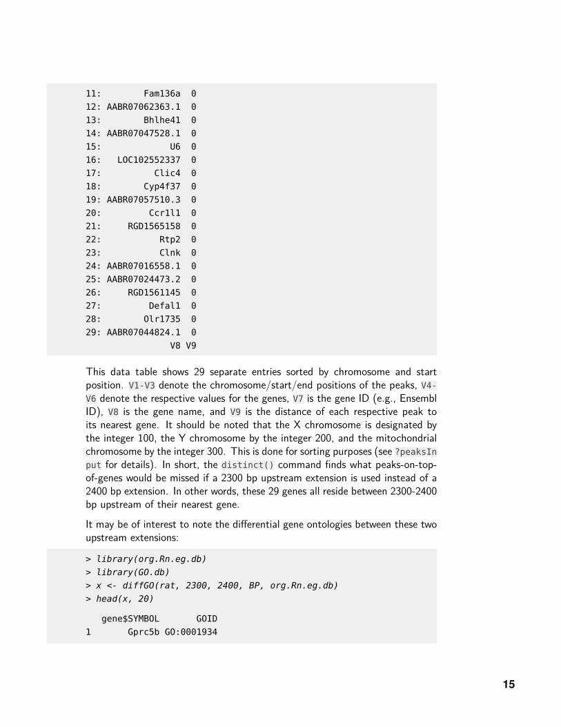
This data table shows 29 separate entries sorted by chromosome and startposition. V1-V3 denote the chromosome/start/end positions of the peaks, V4-V6 denote the respective values for the genes, V7 is the gene ID (e.g., EnsemblID), V8 is the gene name, and V9 is the distance of each respective peak toits nearest gene. It should be noted that the X chromosome is designated bythe integer 100, the Y chromosome by the integer 200, and the mitochondrialchromosome by the integer 300. This is done for sorting purposes (see ?peaksInput for details). In short, the distinct() command finds what peaks-on-top-of-genes would be missed if a 2300 bp upstream extension is used instead of a2400 bp extension. In other words, these 29 genes all reside between 2300-2400bp upstream of their nearest gene.
It may be of interest to note the differential gene ontologies between these twoupstream extensions:
> library(org.Rn.eg.db)
> library(GO.db)
> x <- diffGO(rat, 2300, 2400, BP, org.Rn.eg.db)
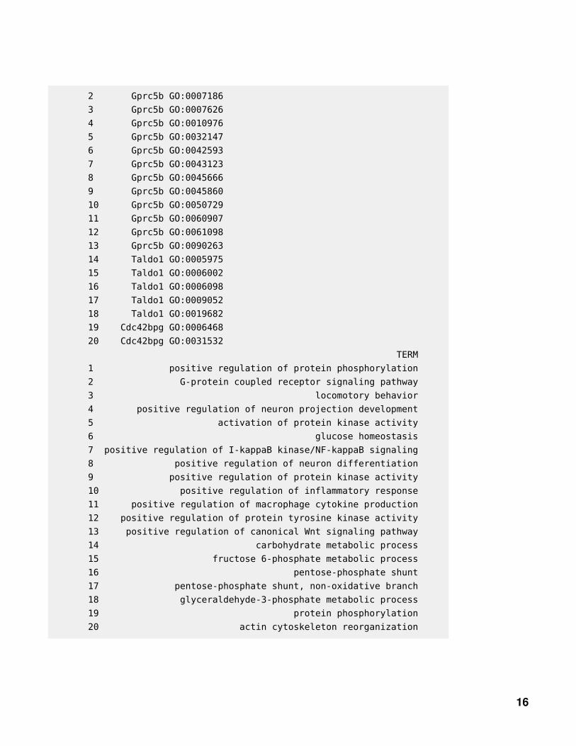
> head(x, 20)
gene$SYMBOL GOID
1 Gprc5b GO:0001934
15
2 Gprc5b GO:0007186
3 Gprc5b GO:0007626
4 Gprc5b GO:0010976
5 Gprc5b GO:0032147
6 Gprc5b GO:0042593
7 Gprc5b GO:0043123
8 Gprc5b GO:0045666
9 Gprc5b GO:0045860
10 Gprc5b GO:0050729
11 Gprc5b GO:0060907
12 Gprc5b GO:0061098
13 Gprc5b GO:0090263
14 Taldo1 GO:0005975
15 Taldo1 GO:0006002
16 Taldo1 GO:0006098
17 Taldo1 GO:0009052
18 Taldo1 GO:0019682
19 Cdc42bpg GO:0006468
20 Cdc42bpg GO:0031532
TERM
1 positive regulation of protein phosphorylation
2 G-protein coupled receptor signaling pathway
3 locomotory behavior
4 positive regulation of neuron projection development
5 activation of protein kinase activity
6 glucose homeostasis
7 positive regulation of I-kappaB kinase/NF-kappaB signaling
8 positive regulation of neuron differentiation
9 positive regulation of protein kinase activity
10 positive regulation of inflammatory response
11 positive regulation of macrophage cytokine production
12 positive regulation of protein tyrosine kinase activity
13 positive regulation of canonical Wnt signaling pathway
14 carbohydrate metabolic process
15 fructose 6-phosphate metabolic process
16 pentose-phosphate shunt
17 pentose-phosphate shunt, non-oxidative branch
18 glyceraldehyde-3-phosphate metabolic process
19 protein phosphorylation
20 actin cytoskeleton reorganization
16
This dataframe shows the first 20 unique gene ontology terms, their IDs, andrespective gene symbols. Clearly, gene name Gprc5b has several BP ontologiesrelated explicitly to the brain, while Taldo1 does not. Considering that the ChIP-seq peaks dataset used as input into geneXtendeR comes from a ChIP-seq studyinvestigating the prefrontal cortex, this suggests that a 2400 bp extension maybe more suitable for this brain dataset. However, such decisions are left entirelyto the discretion and judgment of the user in deciding the relative importanceof specific genes and their respective GO terms (BP, CC, or MF) to the goalsof the computational analysis (as well as plans for experimental follow-up andvalidation). See Discussion section for details.
It is also critical to note that the diffGO() function returns ALL known geneontologies, NOT a gene ontology enrichment analysis (more about this in Dis-cussion section). The goal is to provide users with knowledge regarding all pos-sible known roles of any given gene. For example, by knowing that a potentialgene candidate has previously been linked with known brain-related ontologies,a user may be prompted to look more closely into the relevant literature behindthis gene and its implications to the biological question under study (beforeembarking on making a decision about its potential impact and suitability as agood candidate for experimental validation).
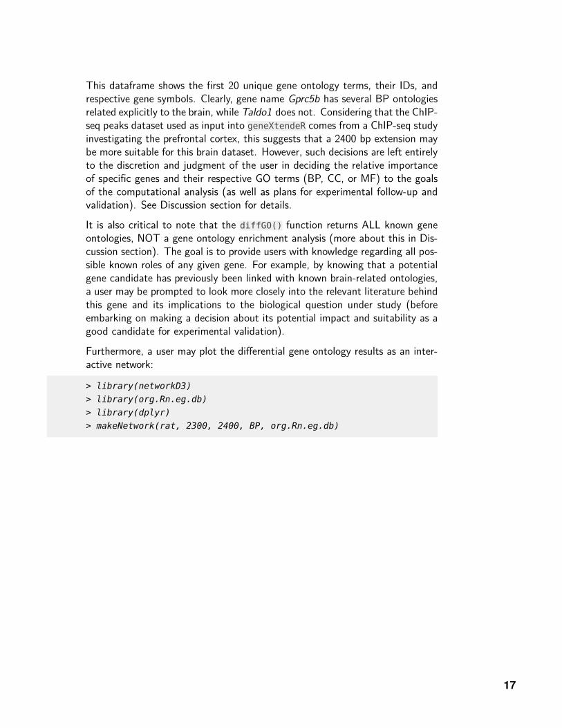
Furthermore, a user may plot the differential gene ontology results as an inter-active network:
> library(networkD3)
> library(org.Rn.eg.db)
> library(dplyr)
> makeNetwork(rat, 2300, 2400, BP, org.Rn.eg.db)
17
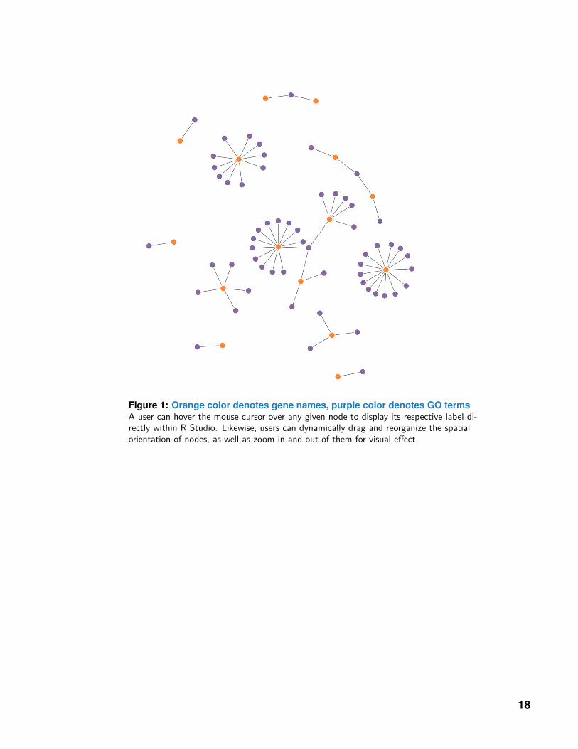
Figure 1: Orange color denotes gene names, purple color denotes GO termsA user can hover the mouse cursor over any given node to display its respective label di-rectly within R Studio. Likewise, users can dynamically drag and reorganize the spatialorientation of nodes, as well as zoom in and out of them for visual effect.
18
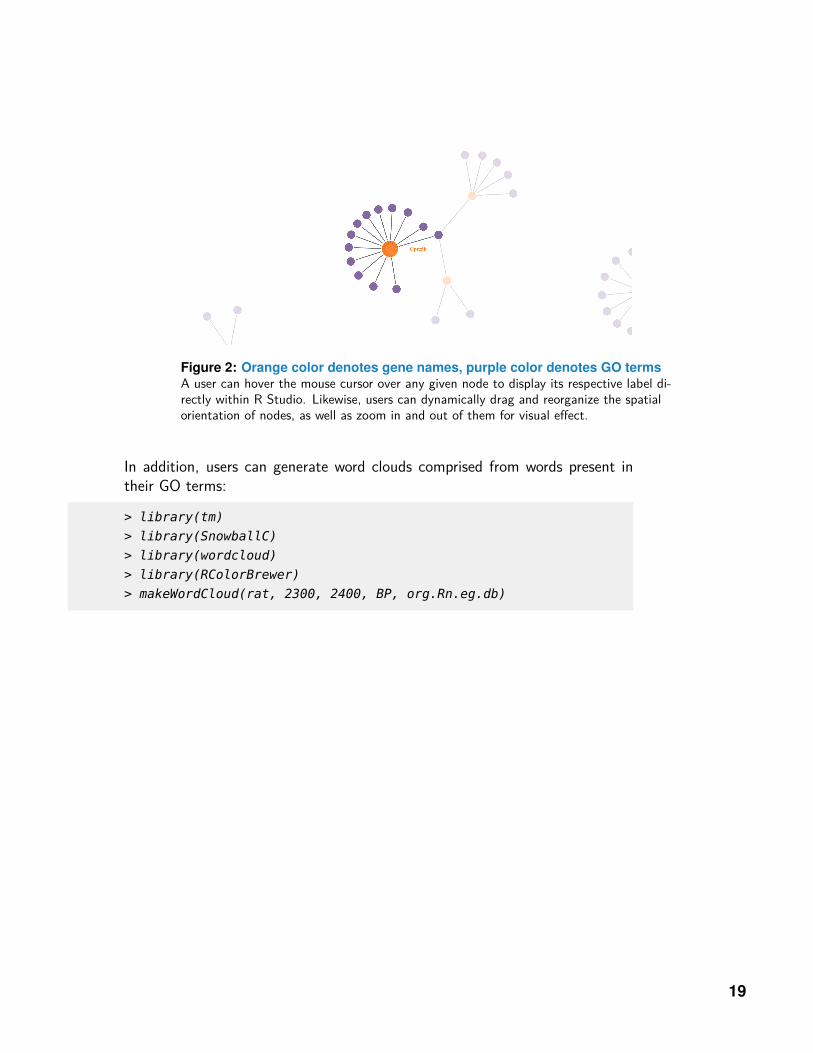
Figure 2: Orange color denotes gene names, purple color denotes GO termsA user can hover the mouse cursor over any given node to display its respective label di-rectly within R Studio. Likewise, users can dynamically drag and reorganize the spatialorientation of nodes, as well as zoom in and out of them for visual effect.
In addition, users can generate word clouds comprised from words present intheir GO terms:
> library(tm)
> library(SnowballC)
> library(wordcloud)
> library(RColorBrewer)
> makeWordCloud(rat, 2300, 2400, BP, org.Rn.eg.db)
19
Figure 3: Word cloud generated from words comprising gene ontology terms ofcategory BPThis word cloud shows the words that are used within BP gene ontology terms of peaksfound to be present between 2300 and 2400 bp upstream of their nearest genes.
It may also be of interest to visually examine the most frequently used wordsfound within GO terms:
> library(tm)
> library(SnowballC)
> library(wordcloud)
> library(RColorBrewer)
> plotWordFreq(rat, 2300, 2400, BP, org.Rn.eg.db, 10)
20
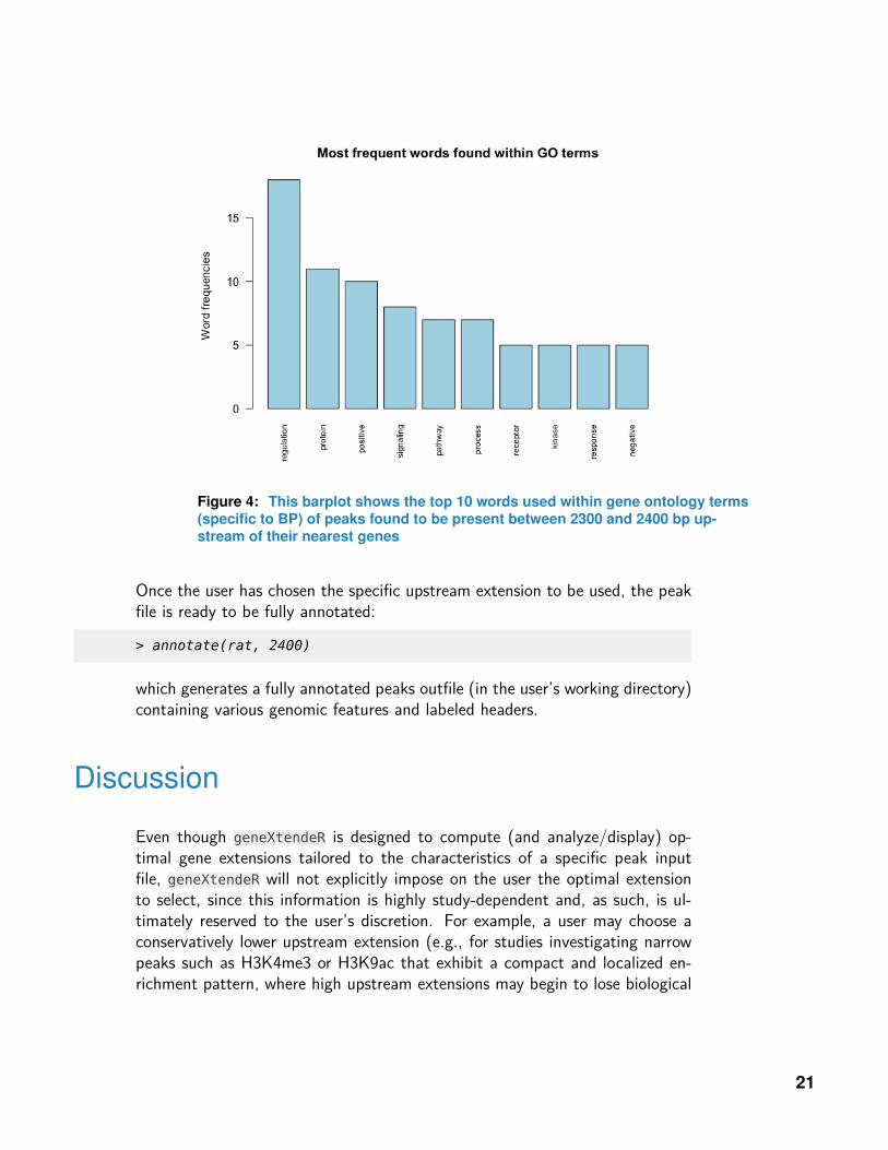
Figure 4: This barplot shows the top 10 words used within gene ontology terms(specific to BP) of peaks found to be present between 2300 and 2400 bp up-stream of their nearest genes
Once the user has chosen the specific upstream extension to be used, the peakfile is ready to be fully annotated:
> annotate(rat, 2400)
which generates a fully annotated peaks outfile (in the user’s working directory)containing various genomic features and labeled headers.
Discussion
Even though geneXtendeR is designed to compute (and analyze/display) op-timal gene extensions tailored to the characteristics of a specific peak inputfile, geneXtendeR will not explicitly impose on the user the optimal extensionto select, since this information is highly study-dependent and, as such, is ul-timately reserved to the user’s discretion. For example, a user may choose aconservatively lower upstream extension (e.g., for studies investigating narrowpeaks such as H3K4me3 or H3K9ac that exhibit a compact and localized en-richment pattern, where high upstream extensions may begin to lose biological
21
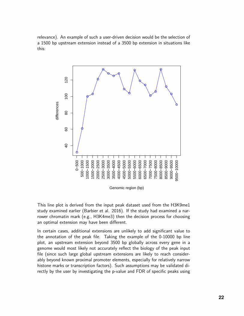
relevance). An example of such a user-driven decision would be the selection ofa 1500 bp upstream extension instead of a 3500 bp extension in situations likethis:
●
●
●●
●
●
●●
●
●
●
●
●
●
●
●
●
●
●
●
4060
8010
012
0
diffe
renc
es
0−50
050
0−10
0010
00−
1500
1500
−20
0020
00−
2500
2500
−30
0030
00−
3500
3500
−40
0040
00−
4500
4500
−50
0050
00−
5500
5500
−60
0060
00−
6500
6500
−70
0070
00−
7500
7500
−80
0080
00−
8500
8500
−90
0090
00−
9500
9500
−10
000
Genomic region (bp)
This line plot is derived from the input peak dataset used from the H3K9me1study examined earlier (Barbier et al. 2016). If the study had examined a nar-rower chromatin mark (e.g., H3K4me3) then the decision process for choosingan optimal extension may have been different.
In certain cases, additional extensions are unlikely to add significant value tothe annotation of the peak file. Taking the example of the 0-10000 bp lineplot, an upstream extension beyond 3500 bp globally across every gene in agenome would most likely not accurately reflect the biology of the peak inputfile (since such large global upstream extensions are likely to reach consider-ably beyond known proximal promoter elements, especially for relatively narrowhistone marks or transcription factors). Such assumptions may be validated di-rectly by the user by investigating the p-value and FDR of specific peaks using
22
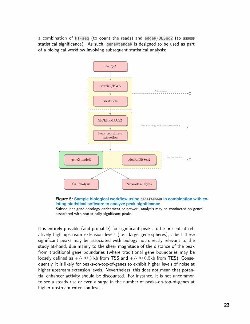
a combination of HT-seq (to count the reads) and edgeR/DESeq2 (to assessstatistical significance). As such, geneXtendeR is designed to be used as partof a biological workflow involving subsequent statistical analysis:
FastQC
Bowtie2/BWA
SAMtools
SICER/MACS2
Peak coordinateextraction
geneXtendeR edgeR/DESeq2
GO analysis Network analysis
Alignment
Peak calling and post-processing
optimization
Figure 5: Sample biological workflow using geneXtendeR in combination with ex-isting statistical software to analyze peak significanceSubsequent gene ontology enrichment or network analysis may be conducted on genesassociated with statistically significant peaks.
It is entirely possible (and probable) for significant peaks to be present at rel-atively high upstream extension levels (i.e., large gene-spheres), albeit thesesignificant peaks may be associated with biology not directly relevant to thestudy at-hand, due mainly to the sheer magnitude of the distance of the peakfrom traditional gene boundaries (where traditional gene boundaries may beloosely defined as +/- ≈ 3 kb from TSS and +/- ≈ 0.5kb from TES). Conse-quently, it is likely for peaks-on-top-of-genes to exhibit higher levels of noise athigher upstream extension levels. Nevertheless, this does not mean that poten-tial enhancer activity should be discounted. For instance, it is not uncommonto see a steady rise or even a surge in the number of peaks-on-top-of-genes athigher upstream extension levels:
23
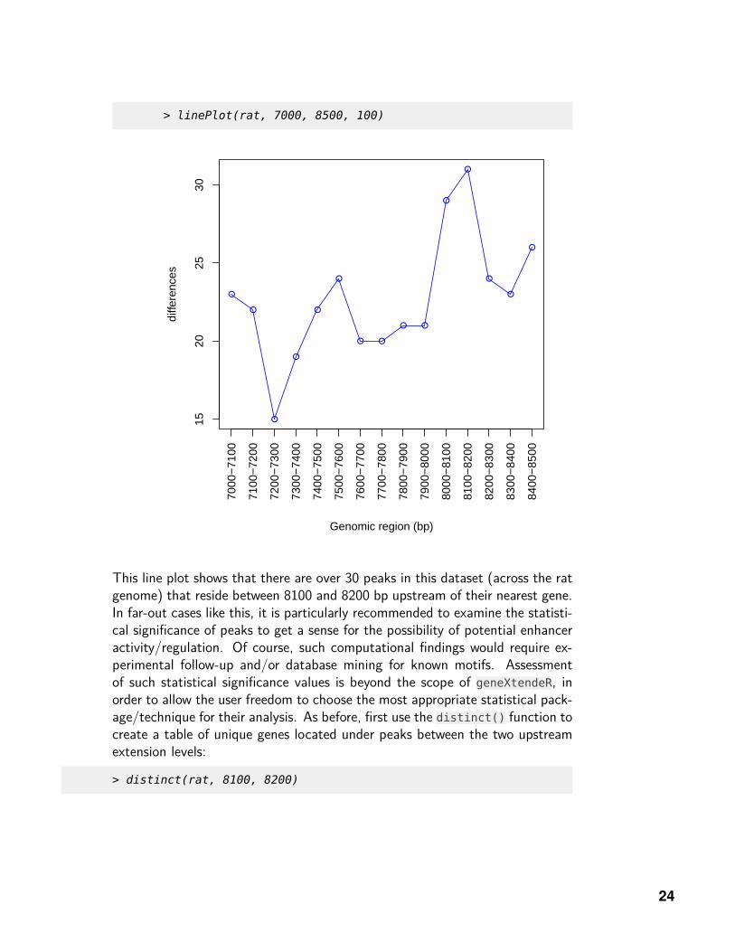
> linePlot(rat, 7000, 8500, 100)
●
●
●
●
●
●
● ●
● ●
●
●
●
●
●
1520
2530
diffe
renc
es
7000
−71
00
7100
−72
00
7200
−73
00
7300
−74
00
7400
−75
00
7500
−76
00
7600
−77
00
7700
−78
00
7800
−79
00
7900
−80
00
8000
−81
00
8100
−82
00
8200
−83
00
8300
−84
00
8400
−85
00Genomic region (bp)
This line plot shows that there are over 30 peaks in this dataset (across the ratgenome) that reside between 8100 and 8200 bp upstream of their nearest gene.In far-out cases like this, it is particularly recommended to examine the statisti-cal significance of peaks to get a sense for the possibility of potential enhanceractivity/regulation. Of course, such computational findings would require ex-perimental follow-up and/or database mining for known motifs. Assessmentof such statistical significance values is beyond the scope of geneXtendeR, inorder to allow the user freedom to choose the most appropriate statistical pack-age/technique for their analysis. As before, first use the distinct() function tocreate a table of unique genes located under peaks between the two upstreamextension levels:
> distinct(rat, 8100, 8200)
24
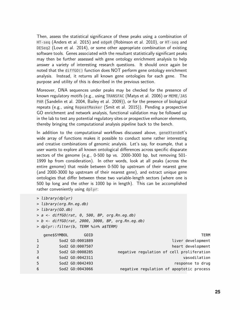
Then, assess the statistical significance of these peaks using a combination ofHT-seq (Anders et al. 2015) and edgeR (Robinson et al. 2010), or HT-seq andDESeq2 (Love et al. 2014), or some other appropriate combination of existingsoftware tools. Genes associated with the resultant statistically significant peaksmay then be further assessed with gene ontology enrichment analysis to helpanswer a variety of interesting research questions. It should once again benoted that the diffGO() function does NOT perform gene ontology enrichmentanalysis. Instead, it returns all known gene ontologies for each gene. Thepurpose and utility of this is described in the previous section.
Moreover, DNA sequences under peaks may be checked for the presence ofknown regulatory motifs (e.g., using TRANSFAC (Matys et al. 2006) or MEME/JASPAR (Sandelin et al. 2004, Bailey et al. 2009)), or for the presence of biologicalrepeats (e.g., using RepeatMasker (Smit et al. 2015)). Pending a prospectiveGO enrichment and network analysis, functional validation may be followed upin the lab to test any potential regulatory sites or prospective enhancer elements,thereby bringing the computational analysis pipeline back to the bench.
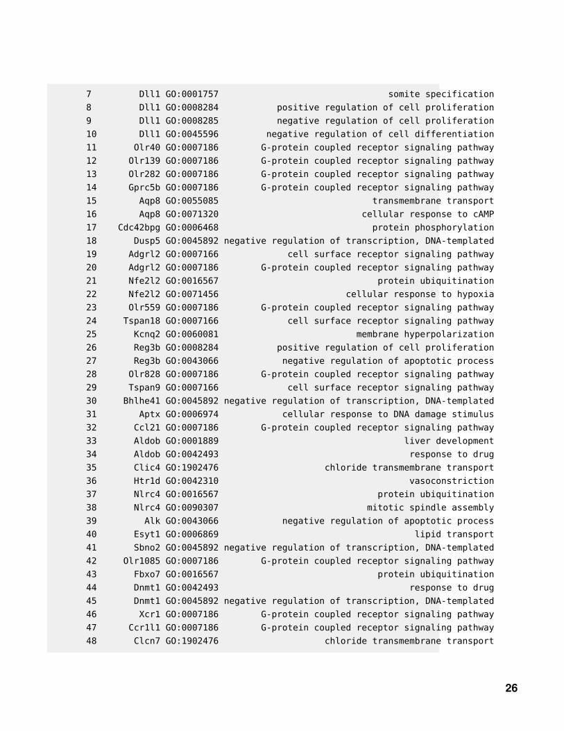
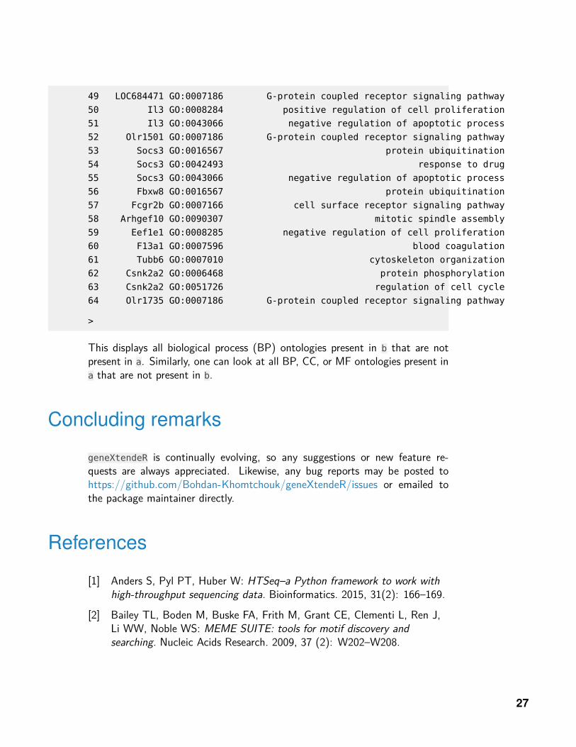
In addition to the computational workflows discussed above, geneXtendeR’swide array of functions makes it possible to conduct some rather interestingand creative combinations of genomic analysis. Let’s say, for example, that auser wants to explore all known ontological differences across specific disparatesectors of the genome (e.g., 0-500 bp vs. 2000-3000 bp, but removing 501-1999 bp from consideration). In other words, look at all peaks (across theentire genome) that reside between 0-500 bp upstream of their nearest gene(and 2000-3000 bp upstream of their nearest gene), and extract unique geneontologies that differ between these two variable-length sectors (where one is500 bp long and the other is 1000 bp in length). This can be accomplishedrather conveniently using dplyr:
> library(dplyr)
> library(org.Rn.eg.db)
> library(GO.db)
> a <- diffGO(rat, 0, 500, BP, org.Rn.eg.db)
> b <- diffGO(rat, 2000, 3000, BP, org.Rn.eg.db)
> dplyr::filter(b, TERM %in% a$TERM)
gene$SYMBOL GOID TERM
1 Sod2 GO:0001889 liver development
2 Sod2 GO:0007507 heart development
3 Sod2 GO:0008285 negative regulation of cell proliferation
4 Sod2 GO:0042311 vasodilation
5 Sod2 GO:0042493 response to drug
6 Sod2 GO:0043066 negative regulation of apoptotic process
25
7 Dll1 GO:0001757 somite specification
8 Dll1 GO:0008284 positive regulation of cell proliferation
9 Dll1 GO:0008285 negative regulation of cell proliferation
10 Dll1 GO:0045596 negative regulation of cell differentiation
11 Olr40 GO:0007186 G-protein coupled receptor signaling pathway
12 Olr139 GO:0007186 G-protein coupled receptor signaling pathway
13 Olr282 GO:0007186 G-protein coupled receptor signaling pathway
14 Gprc5b GO:0007186 G-protein coupled receptor signaling pathway
15 Aqp8 GO:0055085 transmembrane transport
16 Aqp8 GO:0071320 cellular response to cAMP
17 Cdc42bpg GO:0006468 protein phosphorylation
18 Dusp5 GO:0045892 negative regulation of transcription, DNA-templated
19 Adgrl2 GO:0007166 cell surface receptor signaling pathway
20 Adgrl2 GO:0007186 G-protein coupled receptor signaling pathway
21 Nfe2l2 GO:0016567 protein ubiquitination
22 Nfe2l2 GO:0071456 cellular response to hypoxia
23 Olr559 GO:0007186 G-protein coupled receptor signaling pathway
24 Tspan18 GO:0007166 cell surface receptor signaling pathway
25 Kcnq2 GO:0060081 membrane hyperpolarization
26 Reg3b GO:0008284 positive regulation of cell proliferation
27 Reg3b GO:0043066 negative regulation of apoptotic process
28 Olr828 GO:0007186 G-protein coupled receptor signaling pathway
29 Tspan9 GO:0007166 cell surface receptor signaling pathway
30 Bhlhe41 GO:0045892 negative regulation of transcription, DNA-templated
31 Aptx GO:0006974 cellular response to DNA damage stimulus
32 Ccl21 GO:0007186 G-protein coupled receptor signaling pathway
33 Aldob GO:0001889 liver development
34 Aldob GO:0042493 response to drug
35 Clic4 GO:1902476 chloride transmembrane transport
36 Htr1d GO:0042310 vasoconstriction
37 Nlrc4 GO:0016567 protein ubiquitination
38 Nlrc4 GO:0090307 mitotic spindle assembly
39 Alk GO:0043066 negative regulation of apoptotic process
40 Esyt1 GO:0006869 lipid transport
41 Sbno2 GO:0045892 negative regulation of transcription, DNA-templated
42 Olr1085 GO:0007186 G-protein coupled receptor signaling pathway
43 Fbxo7 GO:0016567 protein ubiquitination
44 Dnmt1 GO:0042493 response to drug
45 Dnmt1 GO:0045892 negative regulation of transcription, DNA-templated
46 Xcr1 GO:0007186 G-protein coupled receptor signaling pathway
47 Ccr1l1 GO:0007186 G-protein coupled receptor signaling pathway
48 Clcn7 GO:1902476 chloride transmembrane transport
26
49 LOC684471 GO:0007186 G-protein coupled receptor signaling pathway
50 Il3 GO:0008284 positive regulation of cell proliferation
51 Il3 GO:0043066 negative regulation of apoptotic process
52 Olr1501 GO:0007186 G-protein coupled receptor signaling pathway
53 Socs3 GO:0016567 protein ubiquitination
54 Socs3 GO:0042493 response to drug
55 Socs3 GO:0043066 negative regulation of apoptotic process
56 Fbxw8 GO:0016567 protein ubiquitination
57 Fcgr2b GO:0007166 cell surface receptor signaling pathway
58 Arhgef10 GO:0090307 mitotic spindle assembly
59 Eef1e1 GO:0008285 negative regulation of cell proliferation
60 F13a1 GO:0007596 blood coagulation
61 Tubb6 GO:0007010 cytoskeleton organization
62 Csnk2a2 GO:0006468 protein phosphorylation
63 Csnk2a2 GO:0051726 regulation of cell cycle
64 Olr1735 GO:0007186 G-protein coupled receptor signaling pathway
>
This displays all biological process (BP) ontologies present in b that are notpresent in a. Similarly, one can look at all BP, CC, or MF ontologies present ina that are not present in b.
Concluding remarks
geneXtendeR is continually evolving, so any suggestions or new feature re-quests are always appreciated. Likewise, any bug reports may be posted tohttps://github.com/Bohdan-Khomtchouk/geneXtendeR/issues or emailed tothe package maintainer directly.
References
[1] Anders S, Pyl PT, Huber W: HTSeq–a Python framework to work withhigh-throughput sequencing data. Bioinformatics. 2015, 31(2): 166–169.
[2] Bailey TL, Boden M, Buske FA, Frith M, Grant CE, Clementi L, Ren J,Li WW, Noble WS: MEME SUITE: tools for motif discovery andsearching. Nucleic Acids Research. 2009, 37 (2): W202–W208.
27
[3] Barbier E, Johnstone AL, Khomtchouk BB, Tapocik JD, Pitcairn C,Rehman F, Augier E, Borich A, Schank JR, Rienas CA, Van Booven DJ,Sun H, Nätt D, Wahlestedt C, Heilig M: Dependence-induced increase ofalcohol self-administration and compulsive drinking mediated by thehistone methyltransferase PRDM2. Molecular Psychiatry. 2016, NaturePublishing Group. doi: 10.1038/mp.2016.131.
[4] Heinz S, Benner C, Spann N, Bertolino E et al.: Simple Combinations ofLineage-Determining Transcription Factors Prime cis-RegulatoryElements Required for Macrophage and B Cell Identities. Mol Cell 2010,38(4): 576–589.
[5] Khomtchouk BB, Van Booven DJ, Wahlestedt C: geneXtendeR:R/Bioconductor package for functional annotation of histonemodification ChIP-seq data in a 3D genome world. bioRxiv. 2016, 1–15.
[6] Koohy H, Down TA, Spivakov M, Hubbard T: A Comparison of PeakCallers Used for DNase-Seq Data. PLoS One. 2014, 9(8): e105136.
[7] Love MI, Huber W, Anders S: Moderated estimation of fold change anddispersion for RNA-seq data with DESeq2. Genome Biology. 2014,15:550.
[8] Matys V, Kel-Margoulis OV, Fricke E, Liebich I, Land S, Barre-Dirrie A,Reuter I, Chekmenev D, Krull M, Hornischer K, Voss N, Stegmaier P,Lewicki-Potapov B, Saxel H, Kel AE, Wingender E: TRANSFAC and itsmodule TRANSCompel: transcriptional gene regulation in eukaryotes.2006. Nucleic Acids Research. 34 (Database issue): D108–110.
[9] Quinlan AR, Hall IM: BEDTools: a flexible suite of utilities for comparinggenomic features. Bioinformatics. 2010, 26(6): 841–842.
[10] Robinson MD, McCarthy DJ, Smyth GK: edgeR: a Bioconductor packagefor differential expression analysis of digital gene expression data.Bioinformatics. 2010, 26: 139–140.
[11] Sandelin A, Alkema W, Engstrom P, Wasserman WW, Lenhard B:JASPAR: an open-access database for eukaryotic transcription factorbinding profiles. Nucleic Acids Research. 2004, 32 (Database issue):D91–D94.
[12] Smit AFA, Hubley R, Green P. RepeatMasker Open-4.0. 2013-2015<http://www.repeatmasker.org>.
[13] Thomas R, Thomas S, Holloway AK, Pollard KS: Features that definethe best ChIP-seq peak calling algorithms. Briefings in Bioinformatics.2017, 18(3): 441–450.
28
[14] Zang C, Schones DE, Zeng C, Cui K, Zhao K, Peng W: A clusteringapproach for identification of enriched domains from histone modificationChIP-Seq data. Bioinformatics. 2009, 25(15): 1952–1958.
[15] Zhang Y, Liu T, Meyer CA, Eeckhoute J, Johnson DS, Bernstein BE,Nusbaum C, Myers RM, Brown M, Li W, Liu XS: Model-based analysisof ChIP-Seq (MACS). Genome Biology. 2008, 9(9): R137.
[16] Zhu L, Gazin C, Lawson N, Pages H, Lin S, Lapointe D, Green M:ChIPpeakAnno: a Bioconductor package to annotate ChIP-seq andChIP-chip data. BMC Bioinformatics. 2010, 11(1), pp. 237.
29