Genotype Error Detection using Hidden Markov Models of

Haplotype Diversity∗

Justin Kennedy† Ion Mandoiu† Bogdan Pasaniuc†

July 5, 2008

Abstract

The presence of genotyping errors can invalidate statistical tests for linkage and disease association,

particularly for methods based on haplotype analysis. Becker et al. have recently proposed a simple

likelihood ratio approach for detecting errors in trio genotype data. Under this approach, a SNP genotype

is flagged as a potential error if the likelihood associated with the original trio genotype data increases

by a multiplicative factor exceeding a user selected threshold when the SNP genotype under test is

deleted. In this paper we give improved error detection methods using the likelihood ratio test approach

in conjunction with likelihood functions that can be efficiently computed based on a Hidden Markov

Model of haplotype diversity in the population under study. Experimental results on both simulated and

real datasets show that proposed methods have highly scalable running time and achieve significantly

improved detection accuracy compared to previous methods.

1 Introduction

The sequencing of the human genome coupled with the initial mapping of human haplotypes by the HapMap

project and rapid advances in SNP genotyping technologies have recently opened up the era of genome-wide

∗A preliminary version of this paper will appear in Proc. 7th Workshop on Algorithms in Bioinformatics (WABI), Springer

Verlag Lecture Notes in Computer Science, 2007.

†Computer Science and Engineering Department, University of Connecticut, 371 Fairfield Way, Unit 2155, Storrs, CT

06269-2155. E-mail: {jlk02019,ion,bogdan}@engr.uconn.edu.

1

association studies, which promise to uncover the genetic basis of common complex diseases such as diabetes

and cancer by analyzing the patterns of genetic variation within healthy and diseased individuals. However,

the validity of associations uncovered in these studies critically depends on the accuracy of genotype data.

Despite recent progress in genotype calling algorithms (Cutler et al., 2001; Di et al., 2005; Marchini et al.,

2007; Nicolae et al., 2006; Rabbee & Speed, 2005; Xiao et al., 2007), significant error levels remain present

in SNP genotype data due to factors ranging from human error and sample quality to sequence variation

and assay failure, see (Pompanon et al., 2005) for a recent survey. A recent study of dbSNP genotype data

(Zaitlen et al., 2005) found that as much as 1.1% of about 20 million SNP genotypes typed multiple times

have inconsistent calls, and are thus incorrect in at least one dataset.

Recommended quality control procedures such as the use of external control samples from HapMap and

duplication of internal samples (NCI-NHGRI Working Group on Replication in Association Studies, 2007)

provide an estimate of error rates, but do not eliminate them. Although systematic errors such as assay

failure can be detected by departure from Hardy-Weinberg equilibrium proportions (Hosking et al., 2004;

Leal, 2005), and, when genotype data is available for related individuals, some errors become detectable as

Mendelian Inconsistencies (MIs), a large fraction of errors remains undetected by these analyses, e.g., as

much as 70% of errors in mother-father-child trio genotype data are undetected by Mendelian consistency

analysis (Douglas et al., 2002; Gordon et al., 1999). Since even low error levels can lead to inflated false

positive rates and substantial losses in the statistical power of linkage and association studies (Ahn et al.,

2007; Abecasis et al., 2001; Cherny et al., 2001; Gordon et al., 2002; Mitchell et al., 2003; Zheng & Tian,

2005), detecting Mendelian consistent errors remains a critical task in genetic data analysis. This task

becomes particularly important in the context of association studies based on haplotypes instead of single

locus markers, where error rates as low as 0.1% may invalidate some statistical tests for disease association

(Knapp & Becker, 2004).

A powerful approach of dealing with genotyping errors is to explicitly model them in downstream statis-

tical analyses, see, e.g., (Cheng, 2007; Hao & Wang, 2004; Liu et al., 2007). While powerful, this approach

often leads to complex statistical models and impractical runtime for large datasets such as those generated

by genome-wide association studies. A more practical approach is to perform genotype error detection as

2

a separate analysis step following genotype calling. SNP genotypes flagged as putative errors can be either

excluded from downstream analyses or retyped when high quality genotype data is required. Indeed, such

a separate error detection step is currently implemented in all widely-used software packages for pedigree

genotype data analysis including Mendel (Sobel et al., 2002), Merlin (Abecasis et al., 2002), Sibmed (Dou-

glas et al., 2000), and SimWalk2 (Sobel & Lange, 1996; Sobel et al., 2002), all of which detect Mendelian

consistent errors by independently analyzing each pedigree and identifying loci of excessive recombination.

Unfortunately, these methods have very limited power to detect errors in genotype data from small pedi-

grees such as mother-father-child trios, and do not apply at all to genotype data from unrelated individuals.

(Becker et al., 2006) have recently introduced the use of population level haplotype frequency information

for genotype error detection in trio data via a simple likelihood ratio test. However, detection accuracy of

their method is severely limited by the reliance on explicit enumeration of most frequent haplotypes within

short blocks of consecutive SNP loci.

In this paper we propose novel methods for genotype error detection extending the likelihood ratio error

detection approach of (Becker et al., 2006). While we focus on detecting errors in trio genotype data, our

proposed methods apply with minor modifications to genotype data coming from unrelated individuals and

small pedigrees other than trios. Unlike (Becker et al., 2006), we employ a hidden Markov model (HMM)

to represent frequencies of all possible haplotypes over the set of typed loci. Similar HMMs have been

successfully used in recent works (Kimmel & Shamir, 2005; Rastas et al., 2007; Scheet & Stephens, 2006;

Schwartz, 2004) for genotype phasing and disease association. Two limitations of previous uses of HMMs in

this context have been the relatively slow training based on genotype data and the inability to exploit available

pedigree information. We overcome these limitations by training our HMM using haplotypes inferred by the

pedigree-aware phasing algorithm of (Gusev et al., to appear), based on entropy minimization.

(Becker et al., 2006) use maximum phasing probability of a trio genotype as the likelihood function

whose sensitivity to single SNP genotype deletions signals potential errors. The former is heuristically

approximated by a computationally expensive search over quadruples of frequent haplotypes inferred for each

window. We show that, when haplotype frequencies are implicitly represented using an HMM, computing the

maximum trio phasing probability is, unfortunately, hard to approximate in polynomial time. Despite this

3

hardness result, we are able to significantly improve both detection accuracy and speed compared to (Becker

et al., 2006) by using alternate likelihood functions such as Viterbi probability and the total trio genotype

probability, both of which can be computed for commonly used unrelated and trio genotype data within

a worst-case runtime that increases linearly in the number of SNP loci and that of genotyped individuals.

Further improvements in detection accuracy for genotype trio data are obtained by combining likelihood

ratios computed for different subsets of trio members. Empirical experiments show that this technique is

very effective in reducing false positives within correctly typed SNP genotypes for which the same locus is

mistyped in related individuals.

The rest of the paper is organized as follows. We introduce basic notations in Section 2 describe the

structure of the HMM used to represent haplotype frequencies in Section 3, and present the likelihood ratio

approach of (Becker et al., 2006) in Section 4. In Section 5 we show that the likelihood function in (Becker

et al., 2006) cannot be approximated efficiently when an HMM is used to represent haplotype frequencies,

and then, in Section 6, we give three alternative likelihood functions that can be computed efficiently based

on an HMM. Finally, we give experimental results assessing the error detection accuracy of our methods on

both simulated and real datasets in Section 7, and conclude with ongoing research directions in Section 8.

2 Preliminaries

We start by introducing basic terminology and notations used throughout the paper. We denote the major

and minor alleles at a SNP locus by 0 and 1. A SNP genotype represents the pair of alleles present in an

individual at a SNP locus. Possible SNP genotype values are 0/1/2/?, where 0 and 1 denote homozygous

genotypes for the major and minor alleles, 2 denotes the heterozygous genotype, and ? denotes missing data.

SNP genotype g is said to be explained by an ordered pair of alleles (σ, σ′) ∈ {0, 1}2 if g =?, or g ∈ {0, 1}

and σ = σ′ = g, or g = 2 and σ 6= σ′.

We denote by n the number of SNP loci typed in the population under study. A multi-locus genotype (or

simply genotype) is a 0/1/2/? vector G of length n, while a haplotype is a 0/1 vector H of length n. An ordered

pair (H, H ′) of haplotypes explains multi-locus genotype G iff, for every i = 1, . . . , n, the pair (H(i), H ′(i))

explains G(i). A trio genotype is a triple T = (Gm, Gf , Gc) consisting of mother, father, and child multi-

4

locus genotypes. Assuming that no recombination takes place within the set of SNP loci of interest, we say

that an ordered 4-tuple (H1, H2, H3, H4) of haplotypes explains trio genotype T = (Gm, Gf , Gc) iff (H1, H2)

explains Gm, (H3, H4) explains Gf , and (H1, H3) explains Gc. A genotype duo consisting of mother-child or

father-child genotypes is defined similarly. An ordered 3-tuples of haplotypes (H1, H2, H3) is said to explain

such a duo iff (H1, H2) explains the parent genotype and (H1, H3) explains the child genotype.

3 Hidden Markov ModelFigure 1

belongs

here.

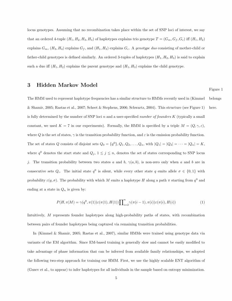
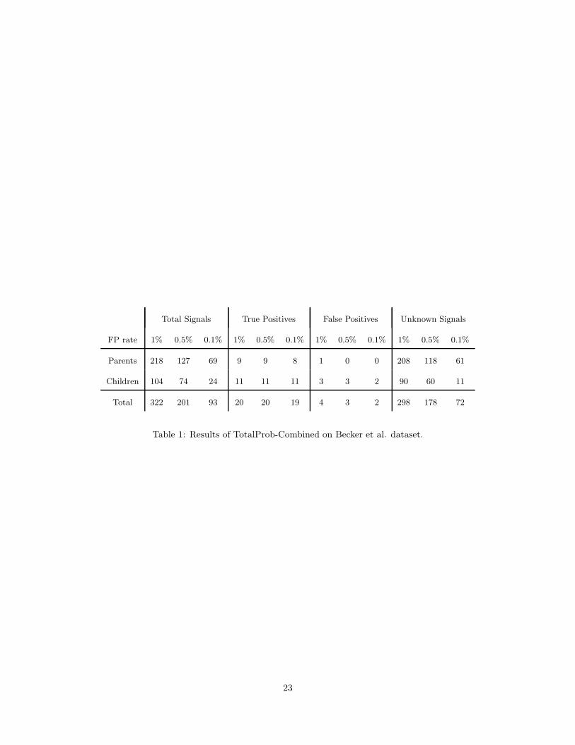
The HMM used to represent haplotype frequencies has a similar structure to HMMs recently used in (Kimmel

& Shamir, 2005; Rastas et al., 2007; Scheet & Stephens, 2006; Schwartz, 2004). This structure (see Figure 1)

is fully determined by the number of SNP loci n and a user-specified number of founders K (typically a small

constant, we used K = 7 in our experiments). Formally, the HMM is specified by a triple M = (Q, γ, ε),

where Q is the set of states, γ is the transition probability function, and ε is the emission probability function.

The set of states Q consists of disjoint sets Q0 = {q0}, Q1, Q2, . . . , Qn, with |Q1| = |Q2| = · · · = |Qn| = K,

where q0 denotes the start state and Qj , 1 ≤ j ≤ n, denotes the set of states corresponding to SNP locus

j. The transition probability between two states a and b, γ(a, b), is non-zero only when a and b are in

consecutive sets Qi. The initial state q0 is silent, while every other state q emits allele σ ∈ {0, 1} with

probability ε(q, σ). The probability with which M emits a haplotype H along a path π starting from q0 and

ending at a state in Qn is given by:

P (H, π|M) = γ(q0, π(1))ε(π(1), H(1))∏n

i=2γ(π(i − 1), π(i))ε(π(i), H(i)) (1)

Intuitively, M represents founder haplotypes along high-probability paths of states, with recombination

between pairs of founder haplotypes being captured via remaining transition probabilities.

In (Kimmel & Shamir, 2005; Rastas et al., 2007), similar HMMs were trained using genotype data via

variants of the EM algorithm. Since EM-based training is generally slow and cannot be easily modified to

take advantage of phase information that can be inferred from available family relationships, we adopted

the following two-step approach for training our HMM. First, we use the highly scalable ENT algorithm of

(Gusev et al., to appear) to infer haplotypes for all individuals in the sample based on entropy minimization.

5

ENT can handle genotypes related by arbitrary pedigrees, and has been shown to yield high phasing accuracy

as measured by the so called switching error, which implies that inferred haplotypes are locally correct with

very high probability. In the second step we use the classical Baum-Welch algorithm (Baum et al., 1970) to

train the HMM based on the haplotypes inferred by ENT.

4 Likelihood ratio approach to genotype error detection

Our detection methods are based on the likelihood ratio approach of (Becker et al., 2006). We call likelihood

function any function L assigning non-negative real-values to trio genotypes, with the further constraint

that L is non-decreasing under data deletion. Let T = (Gm, Gf , Gc) denote a trio genotype, x ∈ {m, f, c}

denote one of the individuals in the trio (mother, father, or child), and i denote one of the n SNP loci. The

trio genotype T(x,i) is obtained from T by marking SNP genotype Gx(i) as missing. The likelihood ratio of

SNP genotype Gx(i) is defined asL(T(x,i))

L(T ) . Notice that, by L’s monotony under data deletion, the likelihood

ratio is always greater or equal to 1. A SNP genotype Gx(i) is flagged as a potential error whenever the

corresponding likelihood ratio exceeds a user specified detection threshold t. A variant of this basic approach

relies on simultaneously testing the mother/father/child SNP genotypes at a locus. In this variant, SNP

locus i is flagged as a potential error whenever L(Ti)L(T ) ≥ t, where Ti is the trio genotype obtained from T by

deleting all three SNP genotypes Gm(i), Gf (i), and Gc(i).

The likelihood function used by Becker et al. (Becker et al., 2006) is the maximum trio phasing probability,

L(T ) = max(H1,H2,H3,H4)

P (H1)P (H2)P (H3)P (H4) (2)

where the above maximum is computed over all 4-tuples (H1, H2, H3, H4) of haplotypes that explain T .

Clearly, the maximum phasing probability is monotonic under data deletion, since deleting SNP genotypes

increases the number of compatible 4-tuples. The use of maximum trio phasing probability as likelihood

function is intuitively appealing, since one does not expect a large increase in this probability when a single

SNP genotype is deleted.

The computational complexity of computing the maximum trio phasing probability L(T ) depends on

the encoding used to represent haplotype frequencies. When the N = 2n haplotype frequencies are given

6

explicitly, computing L(T ) can be trivially done in O(N 4) time. Unfortunately, such an explicit represen-

tation can only be used for a small number n of SNP loci. To maintain practical running time, (Becker

et al., 2006) adopted a heuristic that starts by creating a short list of haplotypes with frequency exceeding

a certain threshold, followed by a pruned search over 4-tuples of haplotypes from this list. Due to the high

computation cost of the search algorithm, the list of haplotypes must be kept very short – between 50 and

100 for the experiments reported in (Becker et al., 2006) – which makes the approach applicable only for

windows of few consecutive SNP loci. This limits the amount of linkage information used in error detection,

explaining at least in part the high number of false positives observed in (Becker et al., 2006) within cor-

rectly typed SNP genotypes located in the neighborhood of SNP genotypes that are mistyped in the same

individual.

The HMM described in previous section provides a much more compact representation of haplotype

frequencies, that can be used for large numbers of SNP loci. Although the probability of any given 4-tuple of

haplotypes explaining a genotype trio can be computed efficiently based on this representation, approximating

the maximum trio phasing probability is shown in next section to be computationally hard. To overcome

this difficulty, in Section 6 we propose alternative likelihood functions that are efficiently computable based

on an HMM representation of haplotype frequencies.

5 Inapproximability of maximum phasing probability

We first consider the problem of computing the maximum phasing probability for a single multi-locus geno-

type:

Maximum genotype phasing probability: Given an HMM model of haplotype diversity with n SNP

loci and K founders and a genotype G ∈ {0, 1, 2, ?}n, find

P (G|M) = max(H1,H2)

P (H1|M)P (H2|M) (3)

where the maximum is computed over all pairs (H1, H2) of haplotypes that explain G.

Theorem 1 Maximum genotype phasing probability cannot be approximated within a factor of O(n12−ε) for

any ε > 0, unless ZPP=NP.

7

Proof. We give a reduction from the problem of computing the size of the maximum clique in an undirected

graph, refining the construction used in (Lyngsø & Pedersen, 2002) to show hardness of approximation for

the consensus string problem.

Let G = (V , E) be a graph with n vertices V = {1, . . . , n}. We will build an HMM MG with n + 1 SNP

loci and a total of K = 4n founders. In addition to the silent start state q0, MG contains for each vertex v

of G and each SNP locus i ∈ {0, 1, . . . , n} four states denoted qiv,j , j = 1, 2, 3, 4 such that qi

v,1 and qiv,3 emit

0 with probability 1, while qiv,2 and qi

v,4 emit 1 with probability 1. For every v ∈ V there are two transitions

from the start state q0 to q0v,2 and q0

v,3, each with probability 2deg(v)

γ, where deg(v) denotes the degree of v

in G and γ =∑

v∈V 2deg(v) is a normalizing constant.

Remaining non-zero probability transitions take place only from a state qi−1v,j to a state qi

v,j′ with ei-

ther j, j′ ∈ {1, 2} or j, j′ ∈ {3, 4}. Non-zero probability transitions within the first two “rows” of states

corresponding to vertex v ∈ V (i.e., states qiv,j with j = 1 and j = 2) are as follows:

• For every SNP locus i ∈ {1, . . . , n} \ {v} such that i is not adjacent to v in G, MG has transitions with

probability 1 from qi−1v,j , j = 1, 2, to qi

v,1

• For every SNP locus i ∈ {1, . . . , n} \ {v} such that i is adjacent to v in G, MG has transitions with

probability 1/2 from qi−1v,j , j = 1, 2, to both qi

v,1 and qiv,2

• Finally, MG has transitions with probability 1 from qv−1v,j , j = 1, 2, to qv

v,2.

By construction, each haplotype emitted along a path within the first two rows of states corresponding to

vertex v consists of a 1 followed by the characteristic vector of one of the 2deg(v) subsets of V that contain v

and zero or more of its neighbors.

Non-zero probability transitions within last two rows of states corresponding to vertex v ∈ V (i.e., states

qiv,j with j = 3 and j = 4) follow a symmetric pattern:

• For every SNP locus i ∈ {1, . . . , n} \ {v} such that i is not adjacent to v, MG has transitions with

probability 1 from qi−1v,j , j = 3, 4, to qi

v,4

• For every SNP locus i ∈ {1, . . . , n}\{v} such that i is adjacent to v, MG has transitions with probability

1/2 from qi−1v,j , j = 3, 4, to both qi

v,3 and qiv,4

8

• MG has transitions with probability 1 from qv−1v,j , j = 3, 4, to qv

v,3.

By construction, haplotypes emitted with non-zero probability along paths within v’s last two rows consist

of a 0 followed by the characteristic vector of the complement of a subset of V that contains v and zero or

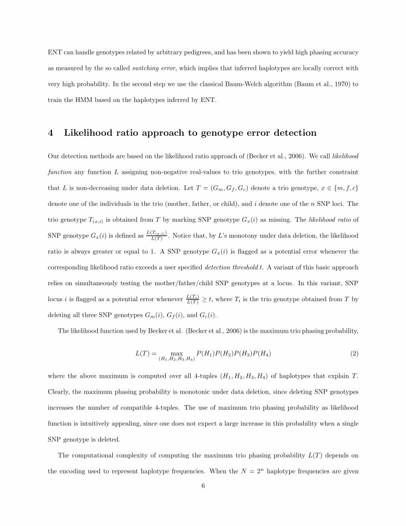
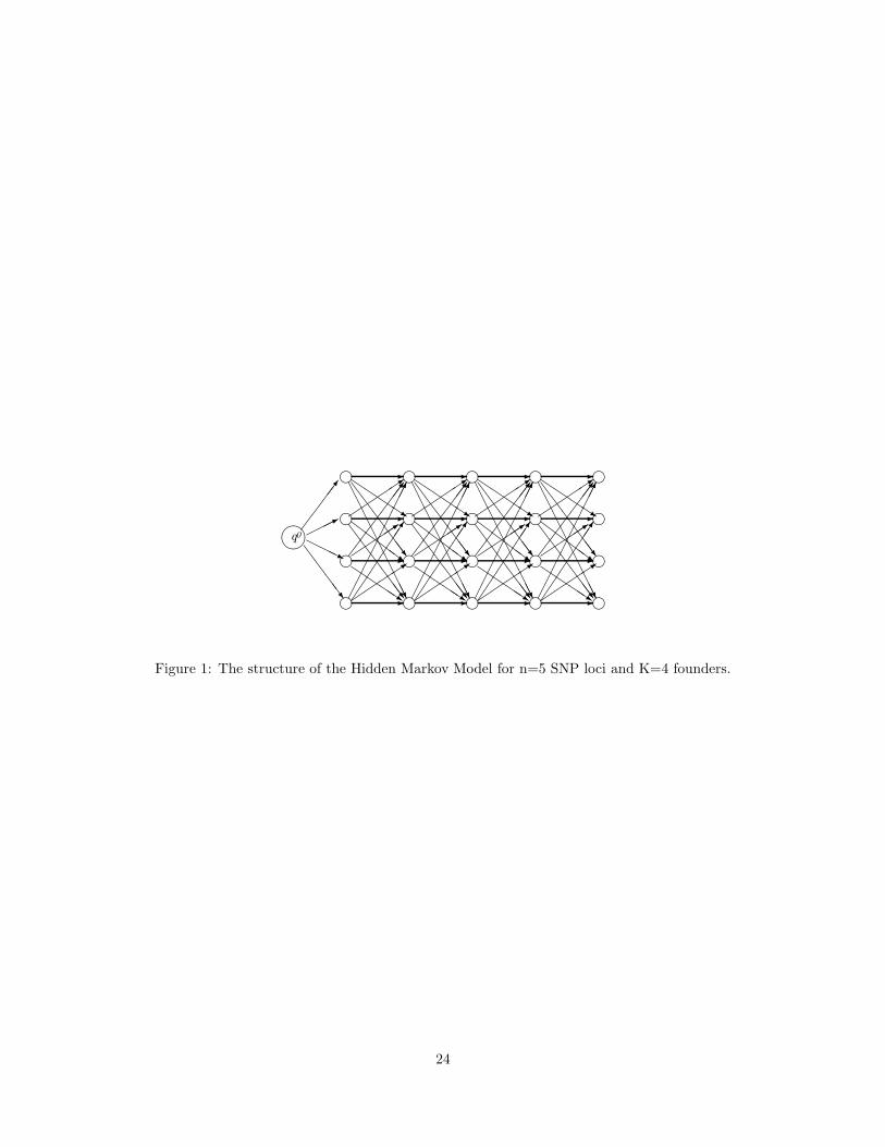
more of its neighbors. To illustrate the construction, Figure 2(b) gives the structure of MG for the simple

graph G in Figure 2(a). Figure 2

belongs

here.

Note that, within the group of states corresponding to vertex v, a haplotype is emitted by MG along

a unique path whose probability 2deg(v)

γ· 1

2deg(v) = 1γ

is independent of v and the haplotype itself. Thus, a

haplotype H consisting of a 1 followed by the characteristic vector of a clique of size k of G is emitted by MG

with probability of k/γ, since there is exactly one path emitting H within each group of states corresponding

to clique vertices. Conversely, any haplotype H starting with 1 that is emitted by MG with probability of

k/γ or more defines a clique of size k or more in G (consisting of vertices v whose groups of states emit H).

Let now G be the multi-locus genotype of length n that is heterozygous at every SNP locus. Clearly, G

can only be explained by pairs (H1, H2) of haplotypes for which H2 = H1, where H denotes the haplotype

obtained by swapping 0’s and 1’s in H . Since the construction of MG implies that P (H |MG) = P (H |MG)

for every haplotype H , it follows that

P (G|MG ) =(

maxH

P (H |MG))2

and therefore G has a clique of size k or more iff P (G|MG) ≥ (k/γ)2. Since clique is hard to approximate

within a factor of O(|V|1−ε) for any ε > 0 unless ZPP=NP (Hastad, 1999), the theorem follows. ut

Remark. Computing maximum phasing probability is closely related to the optimal genotype phasing

problem, which, given an HMM M and a multi-locus genotype G, asks for a pair (H1, H2) of haplotypes

maximizing P (H1|M)P (H2|M). Optimal genotype phasing was conjectured to be NP-hard by (Rastas et al.,

2007). Since computing phasing probability P (H1|M)P (H2|M) can be done in polynomial time for a given

pair (H1, H2) of haplotypes by two runs of the forward algorithm, Theorem 1 trivially extends to the optimal

genotype phasing problem.

The problem of computing the trio-based likelihood function of (Becker et al., 2006) based on an HMM

representation of haplotype frequencies is formalized as follows:

9

Maximum trio phasing probability: Given an HMM model M of haplotype diversity with n SNP loci

and K founders and a trio genotype T = (Gm, Gf , Gc), find

L(T |M) = max(H1,H2,H3,H4)

P (H1|M)P (H2|M)P (H3|M)P (H4|M) (4)

where the maximum is computed over all 4-tuples (H1, H2, H3, H4) of haplotypes that explain T .

Theorem 2 For every ε > 0, maximum trio phasing probability cannot be approximated within a factor of

O(n14−ε) for any ε > 0, unless ZPP=NP.

Proof. We use a reduction similar to that in the proof of Theorem 1. When T consists of three geno-

types that are heterozygous at every locus, the only 4-tuples of haplotypes that explain T are of the form

(H, H, H, H) for some haplotype H . Using the fact that P (H |MG) = P (H |MG) it follows that G has a clique

of size k or more iff P (T |MG) ≥ (k/γ)4, and the theorem follows again from the hardness of approximation

established for the clique problem in (Hastad, 1999). ut

6 Efficiently computable likelihood functions

In this section we consider three alternatives to the likelihood function used in (Becker et al., 2006), and

describe efficient algorithms for computing them given an HMM model of haplotype diversity. As shown in

Section 7, all three alternatives yield similar error detection accuracy, significantly higher than that obtained

in (Becker et al., 2006).

6.1 Viterbi probability

The probability with which the HMM M emits four haplotypes (H1, H2, H3, H4) along a set of 4 paths

(π1, π2, π3, π4) is obtained by a straightforward extension of (1). The first proposed likelihood function is the

Viterbi probability, defined, for a given trio genotype T , as the maximum probability of emitting haplotypes

that explain T along four HMM paths. Viterbi probability can be computed using a “4-path” extension of

the classical Viterbi algorithm (Viterbi, 1967) as follows.

10

For every 4-tuple q = (q1, q2, q3, q4) ∈ Q4j , let Vf (j; q) denote the maximum probability of emitting alleles

that explain the first j SNP genotypes of trio T along a set of 4 paths ending at states (q1, q2, q3, q4) (we will re-

fer to these values as the forward Viterbi values). Also, let Γ(q′, q) = γ(q′1, q1)γ(q′2, q2)γ(q′3, q3)γ(q′4, q4) be the

probability of transition in M from the 4-tuple q′ ∈ Q4j−1 to the 4-tuple q ∈ Q4

j . Then, Vf (0; (q0, q0, q0, q0)) =

1 and

Vf (j; q) = E(j; q) maxq′∈Q4

j−1

{Vf (j − 1; q′)Γ(q′, q)} (5)

Here, E(j; q) = max(σ1,σ2,σ3,σ4)

∏4i=1 ε(qi, σi), where the maximum is computed over all 4-tuples (σ1, σ2, σ3, σ4)

that explain T ’s SNP genotypes at locus j. For a given trio genotype T , the Viterbi probability of T is given

by V (T ) = maxq∈Q4n{Vf (n; q)}.

The time needed to compute forward Viterbi values with the above recurrences is O(nK8), where n

denotes the number of SNP loci and K denotes the number of founders. Indeed, for each one of the O(K4)

4-tuples q ∈ Q4j , computing the maximum in (5) takes O(K4) time. A K3 speed-up is obtained by identifying

and re-using common terms between the maximums (5) corresponding to different 4-tuples q. Thus, instead

of applying (5) directly we compute, for every j, the following:

• m1(j; q1, q′

2, q′

3, q′

4) = maxq′

1∈Qj{Vf (j − 1; (q′1, q

′

2, q′

3, q′

4))γ(q′1, q1)} for each (q1, q′

2, q′

3, q′

4) ∈ Qj × Q3j−1

• m2(j; q1, q2, q′

3, q′

4) = maxq′

2∈Qj{m1(j; (q1, q

′

2, q′

3, q′

4))γ(q′2, q2)} for each (q1, q2, q′

3, q′

4) ∈ Q2j × Q2

j−1

• m3(j; q1, q2, q3, q′

4) = maxq′

3∈Qj

{m2(j; (q1, q2, q′

3, q′

4))γ(q′3, q3)}for each (q1, q2, q3, q′

4) ∈ Q3j × Qj−1

• Vf (j; q) = E(j; q) maxq′

4∈Qj

{m3(j; (q1, q2, q3, q′

4))γ(q′4, q4)} for each q = (q1, q2, q3, q4) ∈ Q4j

A similar speed-up idea was proposed in the context of single genotype phasing by (Rastas et al., 2007).

To apply the likelihood ratio test, we also need to compute Viterbi probabilities for trios with one of

the SNP genotypes deleted. A naıve approach is to compute each of these probabilities from scratch using

the above O(nK5) algorithm. However, this would result in a runtime that grows quadratically with the

number of SNPs. A more efficient algorithm is obtained by also computing backward Viterbi values Vb(j; q),

defined as the maximum probability of emitting alleles that explain genotypes at SNP loci j + 1, . . . , n of

trio T along a set of 4 paths starting at the states of q ∈ Q4j . Once forward and backward Viterbi values

are available, the Viterbi probability of a modified trio can be computed in O(K5) time by using again the

11

above speed-up idea, for an overall runtime of O(nK5) per trio. For unrelated individuals similar speed-up

ideas lead to a runtime of O(nK3) per individual.

6.2 Probability of Viterbi haplotypes

The Viterbi algorithm described in previous section yields, together with the 4 Viterbi paths, a 4-tuple

of haplotypes which we refer to as the Viterbi haplotypes. Viterbi haplotypes for the original trio can be

computed by traceback. Similarly, Viterbi haplotypes corresponding to modified trios can be computed

without increasing the asymptotic runtime via a bi-directional traceback. The second likelihood function

that we considered is the probability of Viterbi haplotypes, which is obtained by multiplying individual

probabilities of Viterbi haplotypes. The probability of each Viterbi haplotype can be computed using the

standard forward algorithm in O(nK) time. Unfortunately, Viterbi paths for modified trios can be completely

different from each other, and the probability of each of them must be computed from scratch by using the

forward algorithm. This results in an overall runtime of O(nK5 +n2K) per trio, respectively O(nK3 +n2K)

per individual for genotype data from unrelated individuals.

6.3 Total trio genotype probability

The third considered likelihood function is the total trio genotype probability, i.e., the total probability P (T )

with which M emits any four haplotypes that explain T along any 4-tuple of paths. Using again the forward

algorithm, P (T ) can be computed as∑

q∈Q4n

p(n; q), where p(0; (q0, q0, q0, q0)) = 1 and

p(j; q) = E(j; q)∑

q′∈Q4j−1

p(j − 1; q′)Γ(q′, q) (6)

The time needed to compute P (T ) with the standard recurrence is O(nK8), but a K3 speed-up can again

be achieved by re-using common terms and computing, in order:

• s1(j; q1, q′

2, q′

3, q′

4) =∑

q′

1∈Qj−1p(j − 1; (q′1, q

′

2, q′

3, q′

4))γ(q′1, q1) for each (q1, q′

2, q′

3, q′

4) ∈ Qj × Q3j−1

• s2(j; q1, q2, q′

3, q′

4) =∑

q′

2∈Qj−1s1(j; (q1, q

′

2, q′

3, q′

4))γ(q′2, q2) for each (q1, q2, q′

3, q′

4) ∈ Q2j × Q2

j−1

• s3(j; q1, q2, q3, q′

4) =∑

q′

3∈Qj−1s2(j; (q1, q2, q

′

3, q′

4))γ(q′3, q3) for each (q1, q2, q3, q′

4) ∈ Q3j × Qj−1

12

• p(j; q) = E(j; q)∑

q′

4∈Qj−1s3(j; (q1, q2, q3, q

′

4))γ(q′4, q4) for each q = (q1, q2, q3, q4) ∈ Q4j

This allows computing P (T |M) in O(nK5) time. By using a forward-backward algorithm, we can obtain

within the same time bound all likelihood ratios for the SNP genotypes in the trio T . For unrelated individuals

the runtime reduces to O(nK3) per individual.

7 Experimental results

7.1 Experimental setup

HMM-based genotype error detection algorithms using the three likelihood functions described in Section 6

were implemented in C++. We tested the performance of our methods on both synthetic datasets and a

real dataset obtained from (Becker et al., 2006). Synthetic datasets were generated as follows. We started

from the real dataset in (Becker et al., 2006), which consists of 551 trios genotyped at 35 SNP loci spanning

a region of 91,391 base pairs from chromosome 16. The FAMHAP software (Becker & Knapp, 2004) was

used to estimate the frequencies of the haplotypes present in the population. The 705 haplotypes that had

positive FAMHAP estimated frequencies were used to derive synthetic datasets with 30-551 trios as follows.

For each trio, four haplotypes were randomly picked by random sampling from the estimated haplotype

frequency distribution. Two of these haplotypes were paired to form the mother genotype, and the other

two were paired to form the father genotype. We created child genotypes by randomly picking from each

parent a transmitted haplotype (assuming that no recombination is taking place). To make the datasets

more realistic, missing data was inserted into the resulting genotypes by replicating the missing data patterns

observed in the real dataset.

Finally, errors were inserted to the genotype data using four models simulating error types generated by

commonly used genotyping technologies (Douglas et al., 2000):

• Random allele model. Under this model, we selected each (trio, SNP locus) pair with a probability of

δ (δ was set to 1% in our experiments). For each selected pair, we picked uniformly at random one of

the non-missing alleles and flipped its value.

• Random genotype model. Again, we selected each (trio, SNP locus) pair with probability δ. For each

13

selected pair, we picked uniformly at random one of the non-missing SNP genotypes and replaced it at

random with one of the two other possible SNP genotypes, according to the expected Hardy-Weinberg

equilibrium genotype frequencies (p2, q2, respectively 2pq for 0, 1, and 2 genotypes, where p is the

estimated probability of allele 0 and q = 1 − p).

• Heterozygous-to-homozygous model. Each heterozygous SNP genotype was selected with probability

δ, and selected genotypes were replaced with equal probability by one of the two homozygous SNP

genotypes.

• Homozygous-to-heterozygous model. Each homozygous SNP genotype was replaced by the heterozygous

SNP genotype with probability δ.

7.2 Results on synthetic datasets

Following the standard practice, we first removed the trivially detected MI errors by marking child SNP

genotypes involved in MIs as missing (similar results were obtained by marking all three SNP genotypes as

missing). To assess error detection accuracy of different methods in a threshold-independent manner we use

receiver operating characteristic (ROC) curves, i.e., plots of achievable sensitivity vs. false positive rates,

where

• the sensitivity is defined as the ratio between the number of Mendelian consistent errors flagged by

the algorithm and the total number of Mendelian consistent errors inserted; and

• the false positive rate is defined as the ratio between the number of non-errors flagged by the algorithm

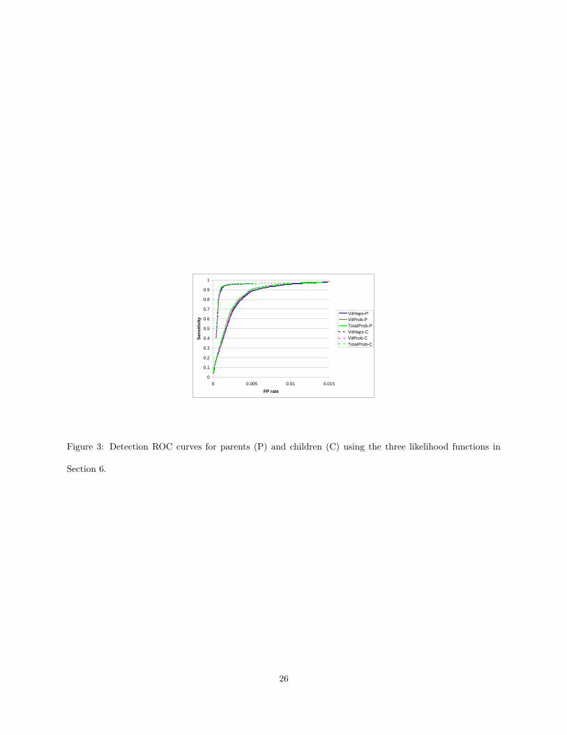
and the total number of non-errors.Figure 3

belongs

here.

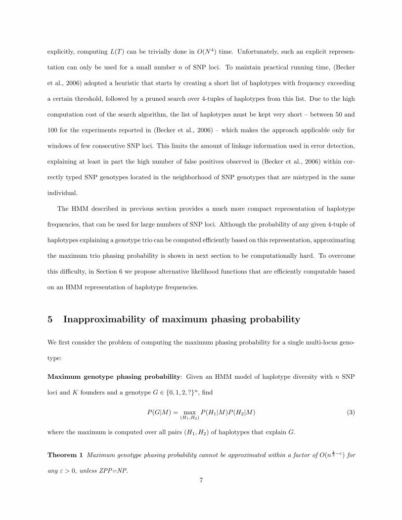
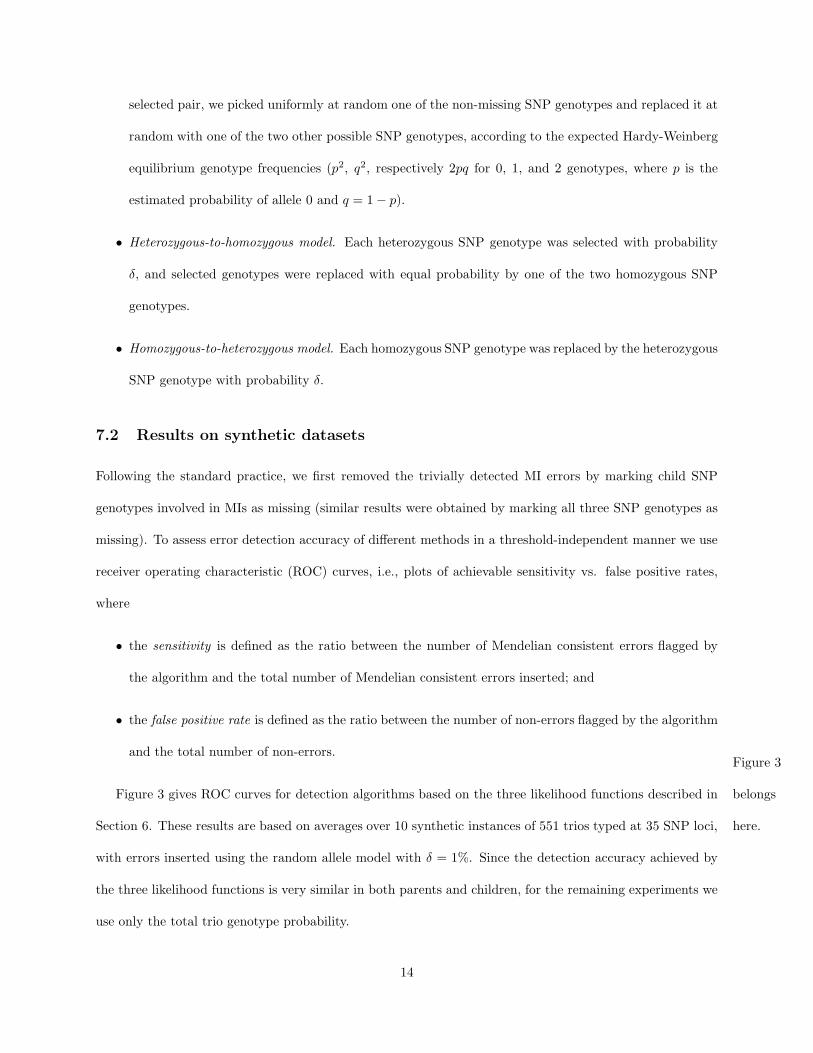
Figure 3 gives ROC curves for detection algorithms based on the three likelihood functions described in

Section 6. These results are based on averages over 10 synthetic instances of 551 trios typed at 35 SNP loci,

with errors inserted using the random allele model with δ = 1%. Since the detection accuracy achieved by

the three likelihood functions is very similar in both parents and children, for the remaining experiments we

use only the total trio genotype probability.

14

It is well known that there is an asymmetry in the amount of information gained from trio genotype

data about children and parent haplotypes: while each of the two child haplotypes are constrained to be

compatible with two genotypes, only one of the parent haplotypes has the same degree of constraint. This

asymmetry is known to make errors in children more likely to result in MIs (Douglas et al., 2002; Gordon

et al., 1999). As shown by the ROC curves in Figure 3, the asymmetry also leads to significantly higher

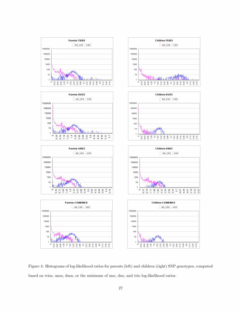
detection sensitivity in children versus parents. Figure 4

belongs

here.

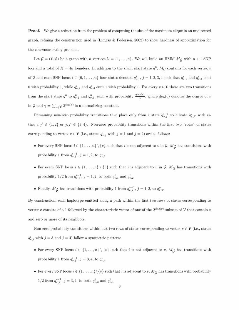
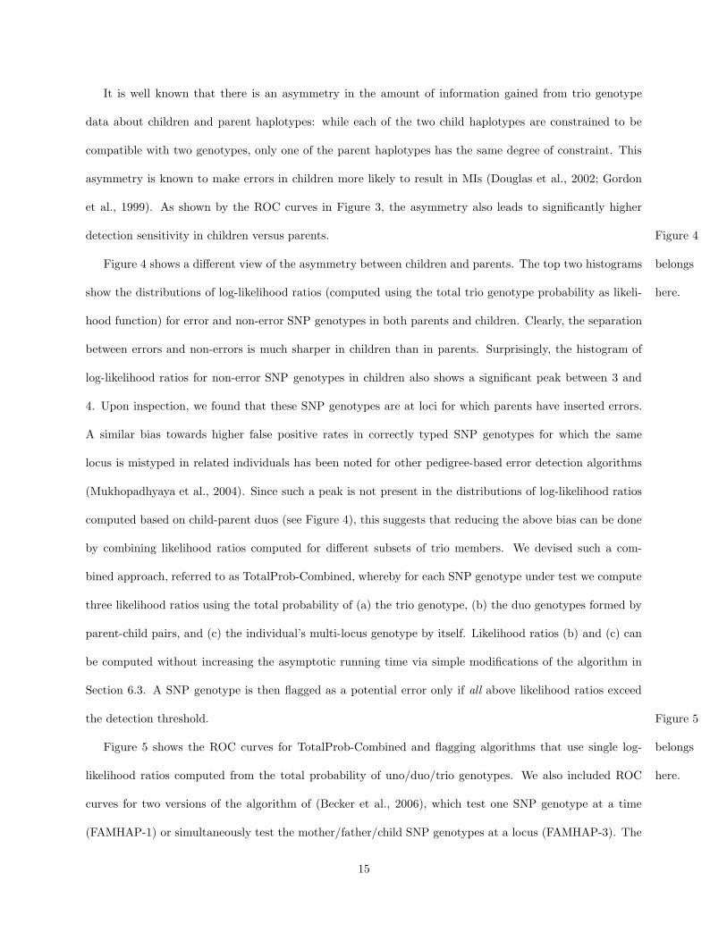
Figure 4 shows a different view of the asymmetry between children and parents. The top two histograms

show the distributions of log-likelihood ratios (computed using the total trio genotype probability as likeli-

hood function) for error and non-error SNP genotypes in both parents and children. Clearly, the separation

between errors and non-errors is much sharper in children than in parents. Surprisingly, the histogram of

log-likelihood ratios for non-error SNP genotypes in children also shows a significant peak between 3 and

4. Upon inspection, we found that these SNP genotypes are at loci for which parents have inserted errors.

A similar bias towards higher false positive rates in correctly typed SNP genotypes for which the same

locus is mistyped in related individuals has been noted for other pedigree-based error detection algorithms

(Mukhopadhyaya et al., 2004). Since such a peak is not present in the distributions of log-likelihood ratios

computed based on child-parent duos (see Figure 4), this suggests that reducing the above bias can be done

by combining likelihood ratios computed for different subsets of trio members. We devised such a com-

bined approach, referred to as TotalProb-Combined, whereby for each SNP genotype under test we compute

three likelihood ratios using the total probability of (a) the trio genotype, (b) the duo genotypes formed by

parent-child pairs, and (c) the individual’s multi-locus genotype by itself. Likelihood ratios (b) and (c) can

be computed without increasing the asymptotic running time via simple modifications of the algorithm in

Section 6.3. A SNP genotype is then flagged as a potential error only if all above likelihood ratios exceed

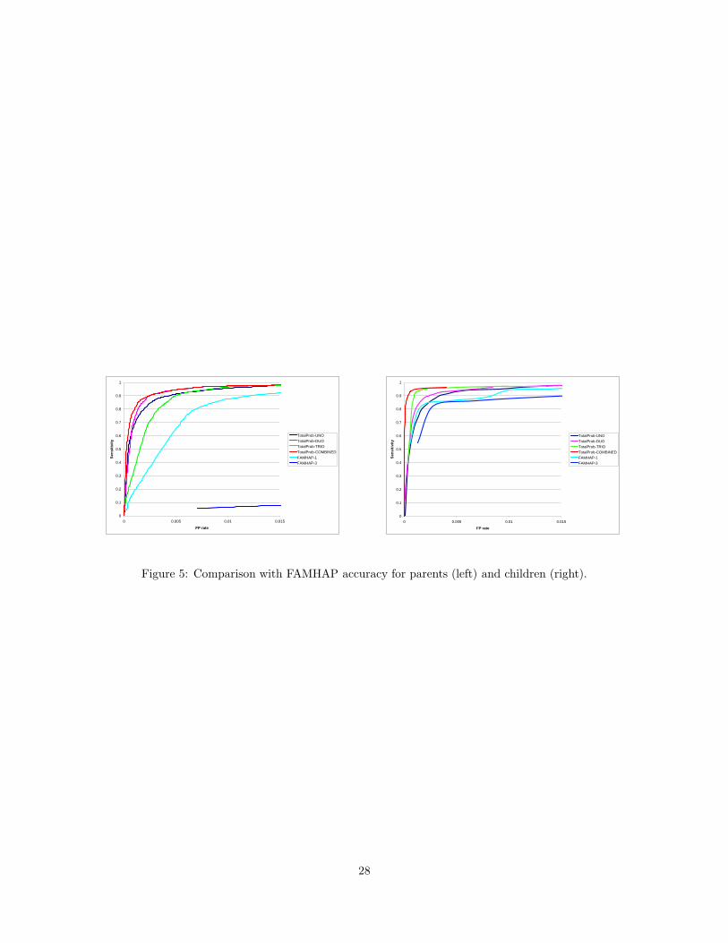
the detection threshold. Figure 5

belongs

here.

Figure 5 shows the ROC curves for TotalProb-Combined and flagging algorithms that use single log-

likelihood ratios computed from the total probability of uno/duo/trio genotypes. We also included ROC

curves for two versions of the algorithm of (Becker et al., 2006), which test one SNP genotype at a time

(FAMHAP-1) or simultaneously test the mother/father/child SNP genotypes at a locus (FAMHAP-3). The

15

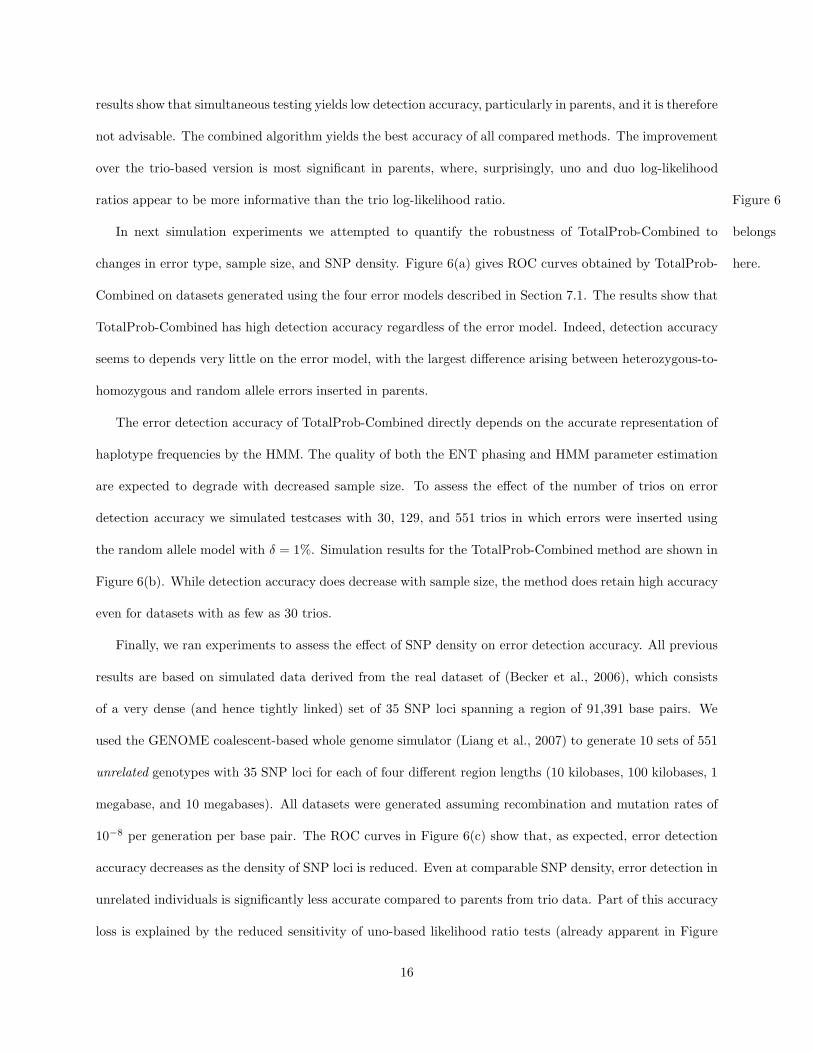
results show that simultaneous testing yields low detection accuracy, particularly in parents, and it is therefore

not advisable. The combined algorithm yields the best accuracy of all compared methods. The improvement

over the trio-based version is most significant in parents, where, surprisingly, uno and duo log-likelihood

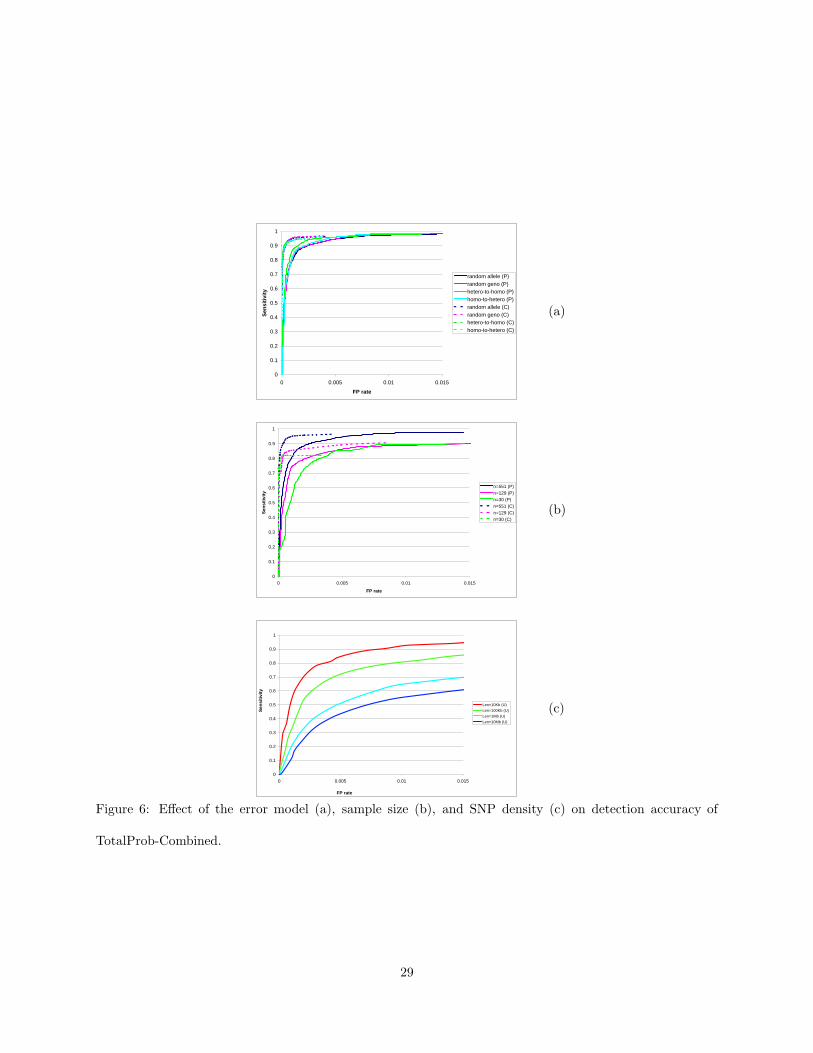
ratios appear to be more informative than the trio log-likelihood ratio. Figure 6

belongs

here.

In next simulation experiments we attempted to quantify the robustness of TotalProb-Combined to

changes in error type, sample size, and SNP density. Figure 6(a) gives ROC curves obtained by TotalProb-

Combined on datasets generated using the four error models described in Section 7.1. The results show that

TotalProb-Combined has high detection accuracy regardless of the error model. Indeed, detection accuracy

seems to depends very little on the error model, with the largest difference arising between heterozygous-to-

homozygous and random allele errors inserted in parents.

The error detection accuracy of TotalProb-Combined directly depends on the accurate representation of

haplotype frequencies by the HMM. The quality of both the ENT phasing and HMM parameter estimation

are expected to degrade with decreased sample size. To assess the effect of the number of trios on error

detection accuracy we simulated testcases with 30, 129, and 551 trios in which errors were inserted using

the random allele model with δ = 1%. Simulation results for the TotalProb-Combined method are shown in

Figure 6(b). While detection accuracy does decrease with sample size, the method does retain high accuracy

even for datasets with as few as 30 trios.

Finally, we ran experiments to assess the effect of SNP density on error detection accuracy. All previous

results are based on simulated data derived from the real dataset of (Becker et al., 2006), which consists

of a very dense (and hence tightly linked) set of 35 SNP loci spanning a region of 91,391 base pairs. We

used the GENOME coalescent-based whole genome simulator (Liang et al., 2007) to generate 10 sets of 551

unrelated genotypes with 35 SNP loci for each of four different region lengths (10 kilobases, 100 kilobases, 1

megabase, and 10 megabases). All datasets were generated assuming recombination and mutation rates of

10−8 per generation per base pair. The ROC curves in Figure 6(c) show that, as expected, error detection

accuracy decreases as the density of SNP loci is reduced. Even at comparable SNP density, error detection in

unrelated individuals is significantly less accurate compared to parents from trio data. Part of this accuracy

loss is explained by the reduced sensitivity of uno-based likelihood ratio tests (already apparent in Figure

16

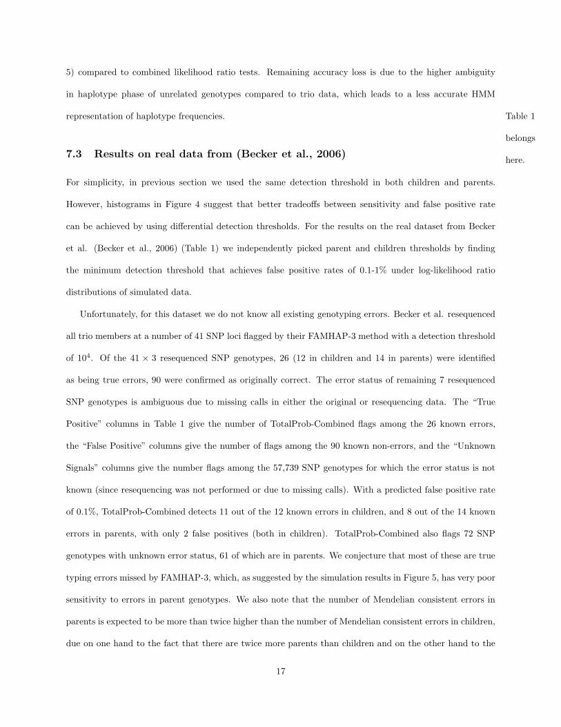
5) compared to combined likelihood ratio tests. Remaining accuracy loss is due to the higher ambiguity

in haplotype phase of unrelated genotypes compared to trio data, which leads to a less accurate HMM

representation of haplotype frequencies. Table 1

belongs

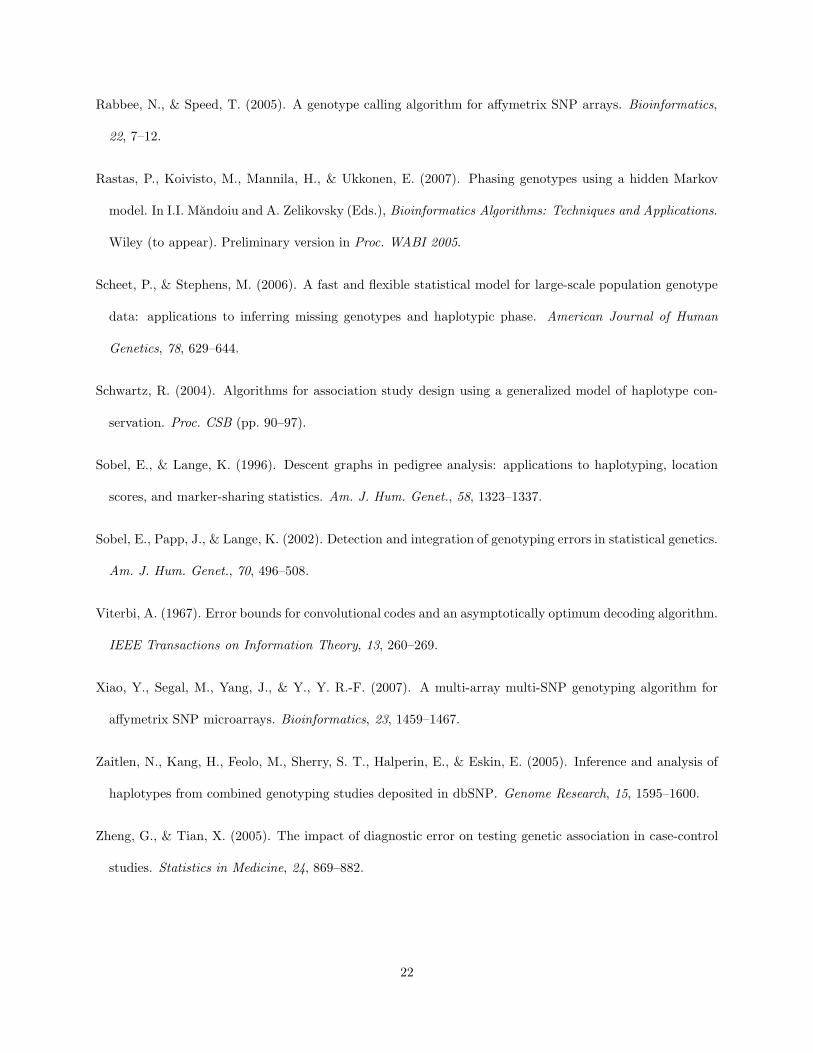
here.7.3 Results on real data from (Becker et al., 2006)

For simplicity, in previous section we used the same detection threshold in both children and parents.

However, histograms in Figure 4 suggest that better tradeoffs between sensitivity and false positive rate

can be achieved by using differential detection thresholds. For the results on the real dataset from Becker

et al. (Becker et al., 2006) (Table 1) we independently picked parent and children thresholds by finding

the minimum detection threshold that achieves false positive rates of 0.1-1% under log-likelihood ratio

distributions of simulated data.

Unfortunately, for this dataset we do not know all existing genotyping errors. Becker et al. resequenced

all trio members at a number of 41 SNP loci flagged by their FAMHAP-3 method with a detection threshold

of 104. Of the 41 × 3 resequenced SNP genotypes, 26 (12 in children and 14 in parents) were identified

as being true errors, 90 were confirmed as originally correct. The error status of remaining 7 resequenced

SNP genotypes is ambiguous due to missing calls in either the original or resequencing data. The “True

Positive” columns in Table 1 give the number of TotalProb-Combined flags among the 26 known errors,

the “False Positive” columns give the number of flags among the 90 known non-errors, and the “Unknown

Signals” columns give the number flags among the 57,739 SNP genotypes for which the error status is not

known (since resequencing was not performed or due to missing calls). With a predicted false positive rate

of 0.1%, TotalProb-Combined detects 11 out of the 12 known errors in children, and 8 out of the 14 known

errors in parents, with only 2 false positives (both in children). TotalProb-Combined also flags 72 SNP

genotypes with unknown error status, 61 of which are in parents. We conjecture that most of these are true

typing errors missed by FAMHAP-3, which, as suggested by the simulation results in Figure 5, has very poor

sensitivity to errors in parent genotypes. We also note that the number of Mendelian consistent errors in

parents is expected to be more than twice higher than the number of Mendelian consistent errors in children,

due on one hand to the fact that there are twice more parents than children and on the other hand to the

17

higher probability that errors in parents remain undetected as Mendelian inconsistencies (Douglas et al.,

2002; Gordon et al., 1999).

8 Conclusions

In this paper we have proposed high-accuracy methods for detection of errors in trio and unrelated genotype

data based on Hidden Markov Models of haplotype diversity. The need for such methods is expected to

increase in the future as genotype analysis methods shift towards the use of haplotypes. The runtime of

our methods scales linearly with the number of trios and SNP loci, making them appropriate for handling

the datasets generated by current large-scale association studies. Our simulation results further indicate the

significant increase in detection accuracy when using genotype data for families of related genotypes such

as trios. Parent-child relationships are well-known to help disambiguating a significant amount of phase

uncertainty by application of simple Mendelian transmission rules. However, our results suggest that the

value of incorporating family relationships in analysis methods can go well beyond these “first order” effects.

A case in point is the sharp increase observed in children genotype error detection sensitivity due to the

use of a trio-based likelihood function. A similar “virtuous cycle” effect was pointed out in ENT phasing

accuracy: not only the number of ambiguous positions decreases significantly when phasing related versus

unrelated genotypes, but the relative phasing accuracy of the algorithm increases significantly as well (Gusev

et al., to appear).

In ongoing work we are extending the TotalProb-Combined method to arbitrary pedigrees. We are also

exploring the use of locus dependent detection thresholds, methods for assigning p-values to error predictions,

and iterative methods which use maximum likelihood to correct MIs and SNP genotypes flagged with a high

detection threshold, then recompute log-likelihoods to flag additional genotypes. Finally, we are exploring

integration of population-level haplotype frequency information with typing confidence scores for further

improvements in error detection accuracy, particularly in the case of unrelated genotype data.

18

Acknowledgments

We would like to thank the authors of (Becker et al., 2006) for kindly providing us the real dataset used

in their paper. This work was supported in part by NSF CAREER award IIS-0546457 and NSF award

DBI-0543365.

References

Abecasis, G., Cherny, S., & Cardon, L. (2001). The impact of genotyping error on family-based analysis of

quantitative traits. Eur. J. Hum. Genet., 9, 130–134.

Abecasis, G., Cherny, S., Cookson, W., & Cardon, L. (2002). Merlin-rapid analysis of dense genetic maps

using sparse gene flow trees. Nat Genet, 30, 97–101.

Ahn, K., Haynes, C., Kim, W., Fleur, R., Gordon, D., & Finch, S. (2007). The effects of SNP genotyping

errors on the power of the Cochran-Armitage linear trend test for case/control association studies. Ann.

Hum. Genet., 71, 249–261.

Baum, L., Petrie, T., Soules, G., & Weiss, N. (1970). A maximization technique occurring in the statistical

analysis of probabilistic functions of Markov chains. Ann. Math. Statist., 41, 164–171.

Becker, T., & Knapp, M. (2004). Maximum-likelihood estimation of haplotype frequencies in nuclear families.

Genet. Epidemiol., 27, 21–32.

Becker, T., Valentonyte, R., Croucher, P., Strauch, K., Schreiber, S., Hampe, J., & Knapp, M. (2006).

Identification of probable genotyping errors by consideration of haplotypes. European Journal of Human

Genetics, 14, 450–458.

Cheng, K. (2007). Analysis of case-only studies accounting for genotyping error. Ann. Hum. Genet., 71,

238–248.

Cherny, S., Abecasis, G., Cookson, W., Sham, P., & Cardon, L. (2001). The effect of genotype and pedigree

error on linkage analysis: Analysis of three asthma genome scans. Genet. Epidemiol., 21, S117–S122.

19

Cutler, D., Zwick, M., Carrasquillo, M., C.T.Yohn, Tobin, K., Kashuk, C., Matthews, D., Shah, N., Eichler,

E., J.A.Warrington, & Chakravarti, A. (2001). High-throughput variation detection and genotyping using

microarrays. Genome Research, 11, 1913–1925.

Di, X., Matsuzaki, H., Webster, T., Hubbell, E., Liu, G., Dong, S., Bartell, D., Huang, J., Chiles, R., Yang,

G., Shen, M.-M., Kulp, D., Kennedy, G., Mei, R., Jones, K., & Cawley, S. (2005). Dynamic model based

algorithms for screening and genotyping over 100k SNPs on oligonucleotide microarrays. Bioinformatics,

21, 1958–1963.

Douglas, J., Boehnke, M., & Lange, K. (2000). A multipoint method for detecting genotyping errors and

mutations in sibling-pair linkage data. AJHG, 66, 1287–1297.

Douglas, J., Skol, A., & Boehnke, M. (2002). Probability of detection of genotyping errors and mutations as

inheritance inconsistencies in nuclear-family data. AJHG, 70, 487–495.

Gordon, D., Finch, S., Nothnagel, M., & Ott, J. (2002). Power and sample size calculations for case-control

genetic association tests when errors are present: Application to single nucleotide polymorphisms. Human

Heredity, 54, 22–33.

Gordon, D., Heath, S., & Ott, J. (1999). True pedigree errors more frequent than apparent errors for single

nucleotide poloymorphisms. Hum. Hered., 49, 65–70.

Gusev, A., Pasaniuc, B., & Mandoiu, I. (to appear). Highly scalable genotype phasing by entropy minimiza-

tion. IEEE/ACM Transactions on Computational Biology and Bioinformatics.

Hao, K., & Wang, X. (2004). Incorporating individual error rate into association test of unmatched case-

control design. Human Heredity, 58, 154–163.

Hastad, J. (1999). Clique is hard to approximate within n1−ε. Acta Mathematica, 182, 105–142.

Hosking, L., Lumsden, S., Lewis, K., Yeo, A., McCarthy, L., Bansal, A., Riley, J., Purvis, I., & Xu, C.

(2004). Detection of genotyping errors by hardy-weinberg equilibrium testing. Eur J. Hum Genet, 12,

395–399.

20

Kimmel, G., & Shamir, R. (2005). A block-free hidden Markov model for genotypes and its application to

disease association. Journal of Computational Biology, 12, 1243–1260.

Knapp, M., & Becker, T. (2004). Impact of genotyping errors on type I error rate of the haplotype-sharing

transmission/disequilibrium test (HS-TDT). Am. J. Hum. Genet., 74, 589–591.

Leal, S. (2005). Detection of genotyping errors and pseudo-SNPs via deviations from Hardy-Weinberg

equilibrium. Genet Epidemiol, 29, 204–214.

Liang, L., Zollner, S., & Abecasis, G. (2007). GENOME: a rapid coalescent-based whole genome simulator.

Bioinformatics, 23, 1565–1567.

Liu, W., Yang, T., Zhao, W., & Chase, G. (2007). Accounting for genotyping errors in tagging SNP selection.

Am. J. Hum. Genet., 71, 467–479.

Lyngsø, R., & Pedersen, C. (2002). The consensus string problem and the complexity of comparing hidden

markov models. J. Comput. Syst. Sci., 65, 545–569.

Marchini, J., Spencer, C., Teo, Y., & Donnelly, P. (2007). A bayesian hierarchical mixture model for genotype

calling in a multi-cohort study. in preparation.

Mitchell, A., Cutler, D., & Chakravarti, A. (2003). Undetected genotyping errors cause apparent overtrans-

mission of common alleles in the transmission/disequilibrium test. Am, J. Hum Genet, 72, 598–610.

Mukhopadhyaya, N., Buxbauma, S., & Weeks, D. (2004). Comparative study of multipoint methods for

genotype error detection. Hum. Hered., 58, 175–189.

NCI-NHGRI Working Group on Replication in Association Studies (2007). Replicating genotype-phenotype

associations. Nature, 447, 655–660.

Nicolae, D., Wu., X., Miyake, K., & Cox, N. (2006). Gel: a novel genotype calling algorithm using emperical

likelihood. Bioinformatics, 22, 1942–1947.

Pompanon, F., Bonin, A., Bellemain, E., & Taberlet, P. (2005). Genotyping errors: causes, consequences

and solutions. Nat. Rev. Genet., 6, 847–859.

21

Rabbee, N., & Speed, T. (2005). A genotype calling algorithm for affymetrix SNP arrays. Bioinformatics,

22, 7–12.

Rastas, P., Koivisto, M., Mannila, H., & Ukkonen, E. (2007). Phasing genotypes using a hidden Markov

model. In I.I. Mandoiu and A. Zelikovsky (Eds.), Bioinformatics Algorithms: Techniques and Applications.

Wiley (to appear). Preliminary version in Proc. WABI 2005.

Scheet, P., & Stephens, M. (2006). A fast and flexible statistical model for large-scale population genotype

data: applications to inferring missing genotypes and haplotypic phase. American Journal of Human

Genetics, 78, 629–644.

Schwartz, R. (2004). Algorithms for association study design using a generalized model of haplotype con-

servation. Proc. CSB (pp. 90–97).

Sobel, E., & Lange, K. (1996). Descent graphs in pedigree analysis: applications to haplotyping, location

scores, and marker-sharing statistics. Am. J. Hum. Genet., 58, 1323–1337.

Sobel, E., Papp, J., & Lange, K. (2002). Detection and integration of genotyping errors in statistical genetics.

Am. J. Hum. Genet., 70, 496–508.

Viterbi, A. (1967). Error bounds for convolutional codes and an asymptotically optimum decoding algorithm.

IEEE Transactions on Information Theory, 13, 260–269.

Xiao, Y., Segal, M., Yang, J., & Y., Y. R.-F. (2007). A multi-array multi-SNP genotyping algorithm for

affymetrix SNP microarrays. Bioinformatics, 23, 1459–1467.

Zaitlen, N., Kang, H., Feolo, M., Sherry, S. T., Halperin, E., & Eskin, E. (2005). Inference and analysis of

haplotypes from combined genotyping studies deposited in dbSNP. Genome Research, 15, 1595–1600.

Zheng, G., & Tian, X. (2005). The impact of diagnostic error on testing genetic association in case-control

studies. Statistics in Medicine, 24, 869–882.

22

Total Signals True Positives False Positives Unknown Signals

FP rate 1% 0.5% 0.1% 1% 0.5% 0.1% 1% 0.5% 0.1% 1% 0.5% 0.1%

Parents 218 127 69 9 9 8 1 0 0 208 118 61

Children 104 74 24 11 11 11 3 3 2 90 60 11

Total 322 201 93 20 20 19 4 3 2 298 178 72

Table 1: Results of TotalProb-Combined on Becker et al. dataset.

23

gg

gg

-Q

QQQs

AAAAAAAAAU

SS

SS

SSw

-

-

-����������

�

��

��3QQ

QQs

��

��3

��

��

��7�

���3

ZZ

ZZ~

SS

SS

SSw

gg

gg

-Q

QQQs

AAAAAAAAAU

SS

SS

SSw

-

-

-����������

�

��

��3QQ

QQs

��

��3

��

��

��7�

���3

ZZ

ZZ~

SS

SS

SSw

gg

gg

-Q

QQQs

AAAAAAAAAU

SS

SS

SSw

-

-

-����������

�

��

��3QQ

QQs

��

��3

��

��

��7�

���3

ZZ

ZZ~

SS

SS

SSw

gg

gg

-Q

QQQs

AAAAAAAAAU

SS

SS

SSw

-

-

-����������

�

��

��3QQ

QQs

��

��3

��

��

��7�

���3

ZZ

ZZ~

SS

SS

SSw

gg

gg

� ��

���*HHHjSS

SSw

��

��7

q0

Figure 1: The structure of the Hidden Markov Model for n=5 SNP loci and K=4 founders.

24

� ��1

� ��3

� ��2

� ��4

@@

@@�

��

�

(a)

l1l0l0

l1-

-

���*-

-HHHj

l0l1

-

- ���*-

-HHHj

l0l1

-

- ���*-

-HHHj

l0l1

-

- ���*-

-HHHj l l l

l lll l l

l

l ll l

l

l ll l

l ll

ll

ll

ll

ll l l

l

l ll l l

l

ll

ll

l

l

l

����

HHHj- ���*

HHHj-

���*���*-

-���*

-HHHj

���*-

HHHj-

���*-

���*-

HHHj-

-HHHj

HHHj-

-

HHHj-

-

HHHj

���*

- ���*-

-���*

-HHHj

���*-

-HHHj

���*

-HHHj

-���*

-HHHj

-

-

-

0

1 1 1

0

0 0 0

1 1

0 0

1 1 1

0

1 1

0

0

1 1 1

0

0

1 1

0

0 0 0

1 1

0 0

1 1

0

1

1

0

1

0

1

0

0

Start

(b)

Figure 2: A sample graph (a) and the corresponding HMM constructed as in the proof of Theorem 1 (b).

The groups of states associated with each vertex are enclosed within dashed boxes. Only states reachable

from the start state are shown, with each non-start state labeled by the allele emitted with probability 1.

25

0

0.1

0.2

0.3

0.4

0.5

0.6

0.7

0.8

0.9

1

0 0.005 0.01 0.015

FP rate

Sen

siti

vity

VitHaps-PVitProb-PTotalProb-PVitHaps-CVitProb-CTotalProb-C

Figure 3: Detection ROC curves for parents (P) and children (C) using the three likelihood functions in

Section 6.

26

Parents-TRIOS

1

10

100

1000

10000

100000

10000000

0.32

0.64

0.96

1.28 1.6

1.92

2.24

2.56

2.88 3.2

3.52

3.84

4.16

4.48 4.8

5.12

5.44

5.76

NO_ERR ERR

Children-TRIOS

1

10

100

1000

10000

100000

1000000

0

0.32

0.64

0.96

1.28 1.6

1.92

2.24

2.56

2.88 3.2

3.52

3.84

4.16

4.48 4.8

5.12

5.44

5.76

NO_ERR ERR

Parents-DUOS

1

10

100

1000

10000

100000

1000000

0

0.38

0.76

1.14

1.52 1.

9

2.28

2.66

3.04

3.42 3.

8

4.18

4.56

4.94

5.32 5.

7

NO_ERR ERR

Children-DUOS

1

10

100

1000

10000

100000

1000000

0

0.32

0.64

0.96

1.28 1.6

1.92

2.24

2.56

2.88 3.2

3.52

3.84

4.16

4.48 4.8

5.12

5.44

5.76

NO_ERR ERR

Parents-UNOS

1

10

100

1000

10000

100000

1000000

0

0.36

0.72

1.08

1.44 1.8

2.16

2.52

2.88

3.24 3.6

3.96

4.32

4.68

5.04 5.4

5.76

NO_ERR ERR

Children-UNOS

1

10

100

1000

10000

100000

1000000

0

0.37

0.74

1.11

1.48

1.85

2.22

2.59

2.96

3.33 3.7

4.07

4.44

4.81

5.18

5.55

5.92

NO_ERR ERR

Parents-COMBINED

1

10

100

1000

10000

100000

1000000

0

0.32

0.64

0.96

1.28 1.6

1.92

2.24

2.56

2.88 3.2

3.52

3.84

4.16

4.48 4.8

5.12

5.44

5.76

NO_ERR ERR

Children-COMBINED

1

10

100

1000

10000

100000

1000000

0

0.32

0.64

0.96

1.28 1.6

1.92

2.24

2.56

2.88 3.2

3.52

3.84

4.16

4.48 4.8

5.12

5.44

5.76

NO_ERR ERR

Figure 4: Histograms of log-likelihood ratios for parents (left) and children (right) SNP genotypes, computed

based on trios, unos, duos, or the minimum of uno, duo, and trio log-likelihood ratios.

27

0

0.1

0.2

0.3

0.4

0.5

0.6

0.7

0.8

0.9

1

0 0.005 0.01 0.015

FP rate

Sen

siti

vity

TotalProb-UNOTotalProb-DUOTotalProb-TRIOTotalProb-COMBINEDFAMHAP-1FAMHAP-3

0

0.1

0.2

0.3

0.4

0.5

0.6

0.7

0.8

0.9

1

0 0.005 0.01 0.015

FP rate

Sen

siti

vity

TotalProb-UNO

TotalProb-DUO

TotalProb-TRIO

TotalProb-COMBINED

FAMHAP-1

FAMHAP-3

Figure 5: Comparison with FAMHAP accuracy for parents (left) and children (right).

28

0

0.1

0.2

0.3

0.4

0.5

0.6

0.7

0.8

0.9

1

0 0.005 0.01 0.015

FP rate

Sen

siti

vity

random allele (P)random geno (P)hetero-to-homo (P)homo-to-hetero (P)random allele (C)random geno (C)hetero-to-homo (C)homo-to-hetero (C)

(a)

0

0.1

0.2

0.3

0.4

0.5

0.6

0.7

0.8

0.9

1

0 0.005 0.01 0.015

FP rate

Sen

siti

vity

n=551 (P)n=129 (P)n=30 (P)n=551 (C)n=129 (C)n=30 (C)

(b)

0

0.1

0.2

0.3

0.4

0.5

0.6

0.7

0.8

0.9

1

0 0.005 0.01 0.015

FP rate

Sen

siti

vity

Len=10Kb (U)

Len=100Kb (U)

Len=1Mb (U)

Len=10Mb (U)

(c)

Figure 6: Effect of the error model (a), sample size (b), and SNP density (c) on detection accuracy of

TotalProb-Combined.

29