Geometric Level Set Methods in Imaging, Vision, and Graphics || Editing Geometric Models

23

Editing Geometric Models

Ken Museth, Ross Whitaker and David Breen

AbstractWe have developed a level set framework for editing closed geometric

models. Level set models are deformable implicit surfaces where the de-formation of the surface is controlled by a speed function in the level setpartial differential equation. In this chapter we define several speed func-tions that provide a set of surface editing operators. The speed functionsdescribe the velocity at each point on the evolving surface in the direction ofthe surface normal. All of the information needed to deform a surface is en-capsulated in the speed function, providing a simple, unified computationalframework. The user combines pre-defined building blocks to create the de-sired speed function. The surface editing operators are quickly computedand may be applied both regionally and globally. The level set frameworkoffers several advantages. 1) By construction, self-intersection cannot occur,which guarantees the generation of physically-realizable, simple, closed sur-faces. 2) Level set models easily change topological genus, and 3) are freeof the edge connectivity and mesh quality problems associated with meshmodels. We present five examples of surface editing operators: blending,smoothing, sharpening, openings/closings and embossing. We demonstratetheir effectiveness on several scanned objects and scan-converted models.

23.1 Introduction

The creation of complex models for such applications as movie special effects,graphic arts, and computer-aided design can be a time-consuming, tedious, anderror-prone process. One of the solutions to the model creation problem is 3Dphotography [61], i.e. scanning a 3D object directly into a digital representation.However, the scanned model is rarely in a final desired form. The scanning pro-cess is imperfect and introduces errors and artifacts, or the object itself may beflawed.

3D scans can be converted to polygonal and parametric surface meshes[174, 26, 17]. Many algorithms and systems for editing these polygonal and

442 Museth, Whitaker & Breen

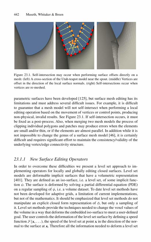
Figure 23.1. Self-intersection may occur when performing surface offsets directly on amesh: (left) A cross-section of the Utah-teapot model near the spout. (middle) Vertices areoffset in the direction of the local surface normals. (right) Self-intersections occur whenvertices are re-meshed.

parametric surfaces have been developed [125], but surface mesh editing has itslimitations and must address several difficult issues. For example, it is difficultto guarantee that a mesh model will not self-intersect when performing a localediting operation based on the movement of vertices or control points, producingnon-physical, invalid results. See Figure 23.1. If self-intersection occurs, it mustbe fixed as a post-process. Also, when merging two mesh models the process ofclipping individual polygons and patches may produce errors when the elementsare small and/or thin, or if the elements are almost parallel. In addition while it isnot impossible to change the genus of a surface mesh model [46], it is certainlydifficult and requires significant effort to maintain the consistency/validity of theunderlying vertex/edge connectivity structure.

23.1.1 New Surface Editing Operators

In order to overcome these difficulties we present a level set approach to im-plementing operators for locally and globally editing closed surfaces. Level setmodels are deformable implicit surfaces that have a volumetric representation[401]. They are defined as an iso-surface, i.e. a level set, of some implicit func-tion �. The surface is deformed by solving a partial differential equation (PDE)on a regular sampling of �, i.e. a volume dataset. To date level set methods havenot been developed for adaptive grids, a limitation of current implementations,but not of the mathematics. It should be emphasized that level set methods do notmanipulate an explicit closed form representation of �, but only a sampling ofit. Level set methods provide the techniques needed to change the voxel values ofthe volume in a way that deforms the embedded iso-surface to meet a user-definedgoal. The user controls the deformation of the level set surface by defining a speedfunction�� ), the speed of the level set at point � in the direction of the nor-mal to the surface at �. Therefore all the information needed to deform a level set

23. Editing Geometric Models 443

model may be encapsulated in a single speed function ��, providing a simple,unified computational framework.

We have developed a number of surface editing operators within a level setframework by defining several new level set speed functions. The cut-and-pasteoperator (Section 23.5.1) gives the user the ability to copy, remove and mergelevel set models (using volumetric CSG operations) and automatically blends theintersection regions (See Section 23.5.2). Our smoothing operator allows a userto define a region of interest and smooths the enclosed surface to a user-definedcurvature value. See Section 23.5.3. We have also developed a point-attractionoperator. See Section 23.5.4. Here, a regionally constrained portion of a level setsurface is attracted to a single point. By defining line segments, curves, polygons,patches and 3D objects as densely sampled point sets, the single point attractionoperator may be combined to produce a more general surface embossing opera-tor. As noted by others, the opening and closing morphological operators may beimplemented in a level set framework [459, 334]. We have also found them use-ful for performing global blending (closing) and smoothing (opening) on level setmodels. Since all of the operators accept and produce the same volumetric repre-sentation of closed surfaces, the operators may be applied repeatedly to producea series of surface editing operations. See Figure 23.11.

23.1.2 Benefits and Issues

Performing surface editing operations within a level set framework provides sev-eral advantages and benefits. Many types of surfaces may be imported into theframework as a distance volume, a volume dataset that stores the signed short-est distance to the surface at each voxel. This allows a number of differenttypes of surfaces to be modified with a single, powerful procedure. By construc-tion, the framework always produces non-self-intersecting surfaces that representphysically-realizable objects, an important issue in computer-aided design. SeeFigure 23.2. Level set models easily change topological genus, and are free ofthe edge connectivity and mesh quality problems associated with deforming andmodifying mesh models. Additionally, some reconstruction algorithms producevolumetric models [144, 573, 609] and volumetric scanning systems are increas-ingly being employed in a number of diverse fields. Therefore volumetric modelsare becoming more prevalent and there is a need to develop powerful editingoperators that act on these types of models directly. There are implementationissues to be addressed when using level set models. Given their volumetric rep-resentation, one may be concerned about the amount of computation time andmemory needed to process level set models. Techniques have been developed tolimit level set computations to only a narrow band around the level set of interest[2, 573, 421] making the computational complexity proportional to the surfacearea of the model. We have also developed computational techniques that allowus to perform the narrow band calculations only in a portion of the volume wherethe level set is actually moving. Additionally, fast marching methods have beendeveloped to rapidly evaluate the level set equation under certain circumstances


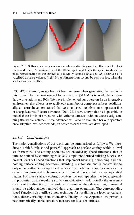
Figure 23.2. Self-intersection cannot occur when performing surface offsets in a level setframework: (left) A cross-section of the Utah-teapot model near the spout. (middle) Im-plicit representation of the surface as a discretly sampled level set, i.e. isosurface of avoxelized distance volume. (right) No self-intersection occurs, by construction, when thelevel set surface is offset.

[533, 473]. Memory usage has not been an issue when generating the results inthis paper. The memory needed for our results (512 MB) is available on stan-dard workstations and PCs. We have implemented our operators in an interactiveenvironment that allows us to easily edit a number of complex surfaces. Addition-ally, concerns have been raised that volume-based models cannot represent fineor sharp features. Recent advances [201, 283] have shown that is is possible tomodel these kinds of structures with volume datasets, without excessively sam-pling the whole volume. These advances will also be available for our operatorsonce adaptive level set methods, an active research area, are developed.

23.1.3 Contributions

The major contributions of our work can be summarized as follows: We intro-duce a unified, robust and powerful approach to surface editing within a levelset framework. The editing operators are encoded by speed functions, that inturn are defined by combining relatively simple pre-defined building blocks. Wepresent level set speed functions that implement blending, smoothing and em-bossing surface editing operators. Blending is automatic and is constrained toonly occur within a user-specified distance to an arbitrarily complex intersectioncurve. Smoothing and embossing are constrained to occur within a user-specifiedregion. For these surface editing operators the user specifies the local geomet-ric properties of the resulting surface modifications. Additionally the user mayconstraint the direction of the surface movements, thus determining if materialshould be added and/or removed during editing operations. The correspondingspeed functions also utilize a new technique for localizing the level set calcula-tions, thereby making them interactive. Finally, in the Appendix, we present anew, numerically-stable curvature measure for level set surfaces.


23.2 Previous Work

Three areas of research are closely related to our level set surface editing work;volumetric sculpting, mesh-based surface editing/fairing and implicit modeling.Volumetric sculpting provides methods for directly manipulating the voxels ofa volumetric model. CSG Boolean operations [241, 560] are commonly foundin volume sculpting systems, providing a straightforward way to create complexsolid objects by combining simpler primitives. One of the first volume sculptingsystems is presented in [205]. [561] improved on this work by introducing toolsfor carving and sawing. More recently [425] implemented a volumetric sculptingsystem based on the Adaptive Distance Fields (ADF) [201], allowing for modelswith adaptive resolution.

Performing CSG operations on mesh models is a long-standing area of research[433, 301]. Recently CSG operations were developed for multi-resolution subdi-vision surfaces by [46], but this work did not address the problem of blendingor smoothing the sharp features often produced by the operations. However, thesmoothing of meshes has been studied on several occasions [572, 509, 284]. [155]have developed a method for fairing irregular meshes using diffusion and curva-ture flow, demonstrating that mean-curvature based flow produces the best resultsfor smoothing.

There exists a large body of surface editing work based on implicit models[55]. This approach uses implicit surface representations of analytic primitives orskeletal offsets. The implicit modeling work most closely related to ours is foundin [582]. They describe techniques for performing blending, warping and booleanoperations on skeletal implicit surfaces. [154] address the converse problem ofpreventing unwanted blending between implicit primitives, as well as maintaininga constant volume during deformation.

Level set methods have been successfully applied in computer graphics,computer vision and visualization [476, 458], for example medical image seg-mentation [331, 574], shape morphing [67], 3D reconstruction [573, 609], andrecently for the animation of liquids [198].

Our work stands apart from previous work in several ways. We have not de-veloped volumetric modeling tools. Our editing operators act on surfaces thathappen to have an underlying volumetric representation, but are based on themathematics of deforming implicit surfaces. Our editing operators share severalof the capabilities of mesh-based tools, but are not hampered by the difficultiesof maintaining vertex/edge information. Since level set models are not tied to anyspecific implicit basis functions, they easily represent complex models to withinthe resolution of the sampling. Our work is the first to utilize level set methods toperform user-controlled editing of complex geometric models.


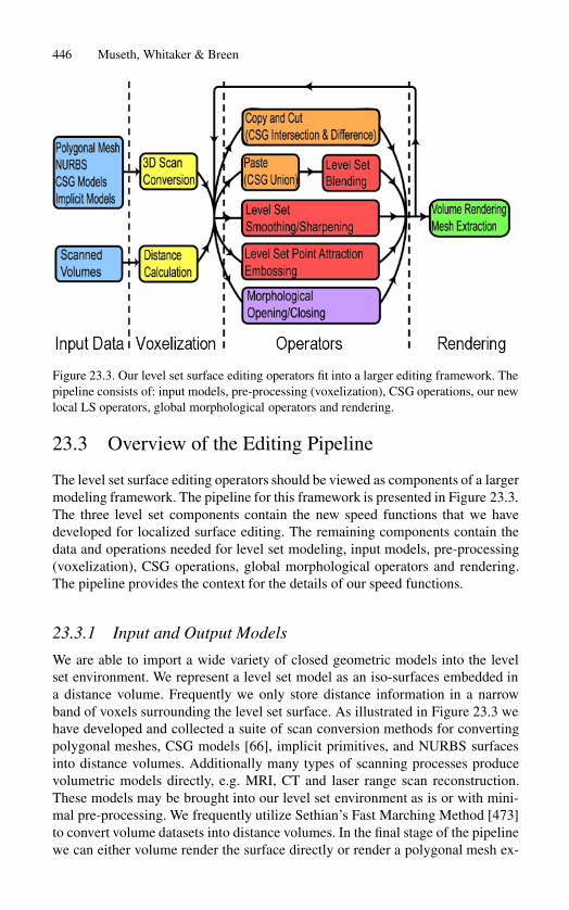
Figure 23.3. Our level set surface editing operators fit into a larger editing framework. Thepipeline consists of: input models, pre-processing (voxelization), CSG operations, our newlocal LS operators, global morphological operators and rendering.

23.3 Overview of the Editing Pipeline

The level set surface editing operators should be viewed as components of a largermodeling framework. The pipeline for this framework is presented in Figure 23.3.The three level set components contain the new speed functions that we havedeveloped for localized surface editing. The remaining components contain thedata and operations needed for level set modeling, input models, pre-processing(voxelization), CSG operations, global morphological operators and rendering.The pipeline provides the context for the details of our speed functions.

23.3.1 Input and Output Models

We are able to import a wide variety of closed geometric models into the levelset environment. We represent a level set model as an iso-surfaces embedded ina distance volume. Frequently we only store distance information in a narrowband of voxels surrounding the level set surface. As illustrated in Figure 23.3 wehave developed and collected a suite of scan conversion methods for convertingpolygonal meshes, CSG models [66], implicit primitives, and NURBS surfacesinto distance volumes. Additionally many types of scanning processes producevolumetric models directly, e.g. MRI, CT and laser range scan reconstruction.These models may be brought into our level set environment as is or with mini-mal pre-processing. We frequently utilize Sethian’s Fast Marching Method [473]to convert volume datasets into distance volumes. In the final stage of the pipelinewe can either volume render the surface directly or render a polygonal mesh ex-


tracted from the volume. While there are numerous techniques available for bothapproaches, we found extracting and rendering Marching Cubes meshes [320] tobe satisfactory.

23.4 Level Set Surface Modeling

The Level Set Method, first presented in [401], can be considered a mathematicaltool for modeling surface deformations. A deformable (i.e. time-dependent) sur-face is implicitly represented as an iso-surface of a time-varying scalar function,�� . A detailed description of level set models is presented in the first chapterof this book.

23.4.1 Level Set Speed Function Building Blocks

Given the definition

��

�� (23.1)

the fundamental level set equation can be written as

��

�� (23.2)

where �� and � � �� are the velocity and normal vectors at � on thesurface. We assume a positive-inside/negative-outside sign convention for �� ,i.e. � points outward. Eq. (23.1) introduces the speed function� , which is a user-defined scalar function that can depend on any number of variables including �,�, � and its derivatives evaluated at �, as well as a variety of external input data.�� is a signed scalar function that defines the motion (i.e. speed) of the level setsurface in the direction of the local normal � at �.

The speed function is usually based on a set of geometric measures of the im-plicit level set surface and input data. The challenge when working with level setmethods is determining how to combine the building blocks to produce a localmotion that creates the desired global or regional behavior of the surface. Thegeneral structure for the speed functions used in our surface editing operators is

�� (23.3)

where �� is a distance-based cut-off function which depends on a distancemeasure � to a geometric structure �. �� is a cut-off function that controls thecontribution of �� to the speed function. �� is a function that depends on geo-metric measures � derived from the level set surface, e.g. curvature. Thus, ��acts as a region-of-influence function that regionally constrains the LS calcula-tion. �� is a filter of the geometric measure and �� provides the geometriccontribution of the level set surface. In general � is defined as zero, first, or secondorder measures of the level set surface.


0.2 0.4 0.6 0.8 1�0.2

0.2

0.4

0.6

0.8

1

Βmin Βmax

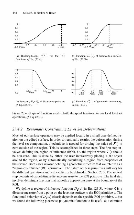
(a) Building-block, � ��, for the ROIfunctions, cf. Eq. (23.4).

-0.5 -0.25 0.25 0.5 0.75 1-0.2

0.2

0.4

0.6

0.8

1

dmin dmax

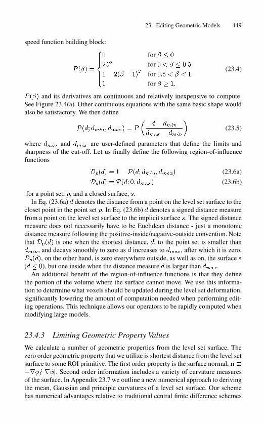
(b) Function, ��, of distance to a surface,cf. Eq. (23.6b).

0.2 0.4 0.6 0.8 1-0.2

0.2

0.4

0.6

0.8

1

dmin dmax

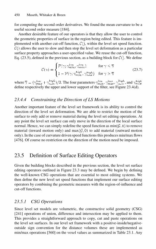
(c) Function, ��, of distance to point set,cf. Eq. (23.6a).

0.2 0.4 0.6 0.8 1�0.2

0.2

0.4

0.6

0.8

1

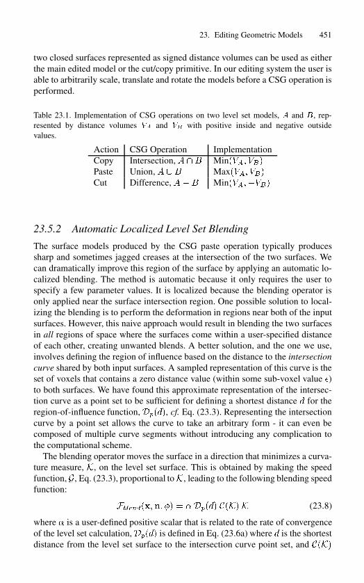
Γminlow Γmax

low Γminhigh Γmax

high

(d) Function, ��, of geometric measure, �,cf. Eq. (23.7).

Figure 23.4. Graph of functions used to build the speed functions for our local level setoperations, cf. Eq. (23.3).

23.4.2 Regionally Constraining Level Set Deformations

Most of our surface operators may be applied locally in a small user-defined re-gion on the edited surface. In order to regionally restrict the deformation duringthe level set computation, a technique is needed for driving the value of �� tozero outside of the region. This is accomplished in three steps. The first step in-volves defining the region of influence (ROI), i.e. the region where �� shouldbe non-zero. This is done by either the user interactively placing a 3D objectaround the region, or by automatically calculating a region from properties ofthe surface. Both cases involve defining a geometric structure that we refer to as a“region-of-influence (ROI) primitive”. The nature of these primitives will vary forthe different operations and will explicitly be defined in Section 23.5. The secondstep consists of calculating a distance measure to the ROI primitive. The final stepinvolves defining a function that smoothly approaches zero at the boundary of theROI.

We define a region-of-influence function �� in Eq. (23.3), where � is adistance measure from a point on the level set surface to the ROI primitive �. Thefunctional behavior of�� clearly depends on the specific ROI primitive, �, butwe found the following piecewise polynomial function to be useful as a common


speed function building block:

� ��

��

� for � � �

�� for � � � � ��

�� for ��

� for � � ��

(23.4)

� �� and its derivatives are continuous and relatively inexpensive to compute.See Figure 23.4(a). Other continuous equations with the same basic shape wouldalso be satisfactory. We then define

��

��

��

�(23.5)

where �� and �� are user-defined parameters that define the limits andsharpness of the cut-off. Let us finally define the following region-of-influencefunctions

�� (23.6a)

�� (23.6b)

for a point set, �, and a closed surface, �.In Eq. (23.6a) � denotes the distance from a point on the level set surface to the

closet point in the point set �. In Eq. (23.6b) � denotes a signed distance measurefrom a point on the level set surface to the implicit surface �. The signed distancemeasure does not necessarily have to be Euclidean distance - just a monotonicdistance measure following the positive-inside/negative-outside convention. Notethat �� is one when the shortest distance, �, to the point set is smaller than��, and decays smoothly to zero as � increases to ��, after which it is zero.��, on the other hand, is zero everywhere outside, as well as on, the surface �(� � �), but one inside when the distance measure � is larger than ��.

An additional benefit of the region-of-influence functions is that they definethe portion of the volume where the surface cannot move. We use this informa-tion to determine what voxels should be updated during the level set deformation,significantly lowering the amount of computation needed when performing edit-ing operations. This technique allows our operators to be rapidly computed whenmodifying large models.

23.4.3 Limiting Geometric Property Values

We calculate a number of geometric properties from the level set surface. Thezero order geometric property that we utilize is shortest distance from the level setsurface to some ROI primitive. The first order property is the surface normal, � ��. Second order information includes a variety of curvature measuresof the surface. In Appendix 23.7 we outline a new numerical approach to derivingthe mean, Gaussian and principle curvatures of a level set surface. Our schemehas numerical advantages relative to traditional central finite difference schemes


for computing the second order derivatives. We found the mean curvature to be auseful second order measure [184].

Another desirable feature of our operators is that they allow the user to controlthe geometric properties of surface in the region being edited. This feature is im-plemented with another cut-off function, ��, within the level set speed function.�� allows the user to slow and then stop the level set deformation as a particularsurface property approaches a user-specified value. We reuse the cut-off function,Eq. (23.5), defined in the previous section, as a building block for ��. We define

��

��

�� for � � �

�� for � � �

(23.7)

where � � �� . The four parameters ��, ��, �� , and ��

define respectively the upper and lower support of the filter, see Figure 23.4(d).

23.4.4 Constraining the Direction of LS Motions

Another important feature of the level set framework is its ability to control thedirection of the level set deformation. We are able to restrict the motion of thesurface to only add or remove material during the level set editing operations. Atany point the level set surface can only move in the direction of the local surfacenormal. Hence, we can simply redefine the speed function as min�� to removematerial (inward motion only) and max�� to add material (outward motiononly). In the case of curvature driven speed functions this produces min/max flows[476]. Of course no restriction on the direction of the motion need be imposed.

23.5 Definition of Surface Editing Operators

Given the building blocks described in the previous section, the level set surfaceediting operators outlined in Figure 23.3 may be defined. We begin by definingthe well-known CSG operations that are essential to most editing systems. Wethen define the new level set speed functions that implement our surface editingoperators by combining the geometric measures with the region-of-influence andcut-off functions.

23.5.1 CSG Operations

Since level set models are volumetric, the constructive solid geometry (CSG)[241] operations of union, difference and intersection may be applied to them.This provides a straightforward approach to copy, cut and paste operations onthe level set surfaces. In our level set framework with a positive-inside/negative-outside sign convention for the distance volumes these are implemented asmin/max operations [560] on the voxel values as summarized in Table 23.1. Any


two closed surfaces represented as signed distance volumes can be used as eitherthe main edited model or the cut/copy primitive. In our editing system the user isable to arbitrarily scale, translate and rotate the models before a CSG operation isperformed.

Table 23.1. Implementation of CSG operations on two level set models, � and �, rep-resented by distance volumes �� and �� with positive inside and negative outsidevalues.

Action CSG Operation ImplementationCopy Intersection, � � � Min�� Paste Union, � � � Max�� Cut Difference, �� Min��

23.5.2 Automatic Localized Level Set Blending

The surface models produced by the CSG paste operation typically producessharp and sometimes jagged creases at the intersection of the two surfaces. Wecan dramatically improve this region of the surface by applying an automatic lo-calized blending. The method is automatic because it only requires the user tospecify a few parameter values. It is localized because the blending operator isonly applied near the surface intersection region. One possible solution to local-izing the blending is to perform the deformation in regions near both of the inputsurfaces. However, this naive approach would result in blending the two surfacesin all regions of space where the surfaces come within a user-specified distanceof each other, creating unwanted blends. A better solution, and the one we use,involves defining the region of influence based on the distance to the intersectioncurve shared by both input surfaces. A sampled representation of this curve is theset of voxels that contains a zero distance value (within some sub-voxel value �)to both surfaces. We have found this approximate representation of the intersec-tion curve as a point set to be sufficient for defining a shortest distance � for theregion-of-influence function, ��, cf. Eq. (23.3). Representing the intersectioncurve by a point set allows the curve to take an arbitrary form - it can even becomposed of multiple curve segments without introducing any complication tothe computational scheme.

The blending operator moves the surface in a direction that minimizes a curva-ture measure, �, on the level set surface. This is obtained by making the speedfunction, �, Eq. (23.3), proportional to�, leading to the following blending speedfunction:

�� (23.8)

where � is a user-defined positive scalar that is related to the rate of convergenceof the level set calculation,�� is defined in Eq. (23.6a) where � is the shortestdistance from the level set surface to the intersection curve point set, and ��


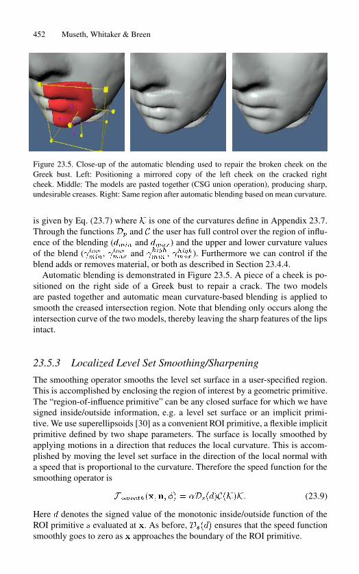
Figure 23.5. Close-up of the automatic blending used to repair the broken cheek on theGreek bust. Left: Positioning a mirrored copy of the left cheek on the cracked rightcheek. Middle: The models are pasted together (CSG union operation), producing sharp,undesirable creases. Right: Same region after automatic blending based on mean curvature.

is given by Eq. (23.7) where � is one of the curvatures define in Appendix 23.7.Through the functions�� and � the user has full control over the region of influ-ence of the blending (�� and ��) and the upper and lower curvature valuesof the blend (��, �� and �

�� , �� ). Furthermore we can control if the

blend adds or removes material, or both as described in Section 23.4.4.Automatic blending is demonstrated in Figure 23.5. A piece of a cheek is po-

sitioned on the right side of a Greek bust to repair a crack. The two modelsare pasted together and automatic mean curvature-based blending is applied tosmooth the creased intersection region. Note that blending only occurs along theintersection curve of the two models, thereby leaving the sharp features of the lipsintact.

23.5.3 Localized Level Set Smoothing/Sharpening

The smoothing operator smooths the level set surface in a user-specified region.This is accomplished by enclosing the region of interest by a geometric primitive.The “region-of-influence primitive” can be any closed surface for which we havesigned inside/outside information, e.g. a level set surface or an implicit primi-tive. We use superellipsoids [30] as a convenient ROI primitive, a flexible implicitprimitive defined by two shape parameters. The surface is locally smoothed byapplying motions in a direction that reduces the local curvature. This is accom-plished by moving the level set surface in the direction of the local normal witha speed that is proportional to the curvature. Therefore the speed function for thesmoothing operator is

�� (23.9)

Here � denotes the signed value of the monotonic inside/outside function of theROI primitive � evaluated at �. As before, �� ensures that the speed functionsmoothly goes to zero as � approaches the boundary of the ROI primitive.


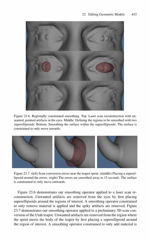
Figure 23.6. Regionally constrained smoothing. Top: Laser scan reconstruction with un-wanted, pointed artifacts in the eyes. Middle: Defining the regions to be smoothed with twosuperellipsoids. Bottom: Smoothing the surface within the superellipsoids. The surface isconstrained to only move inwards.

Figure 23.7. (left) Scan conversion errors near the teapot spout. (middle) Placing a superel-lipsoid around the errors. (right) The errors are smoothed away in 15 seconds. The surfaceis constrained to only move outwards.

Figure 23.6 demonstrates our smoothing operator applied to a laser scan re-construction. Unwanted artifacts are removed from the eyes by first placingsuperellipsoids around the regions of interest. A smoothing operator constrainedto only remove material is applied and the spiky artifacts are removed. Figure23.7 demonstrates our smoothing operator applied to a preliminary 3D scan con-version of the Utah teapot. Unwanted artifacts are removed from the region wherethe spout meets the body of the teapot by first placing a superellipsoid aroundthe region of interest. A smoothing operator constrained to only add material is


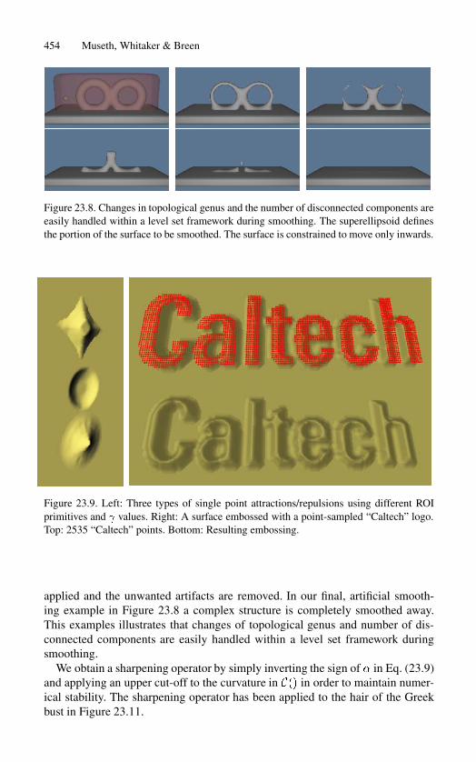
Figure 23.8. Changes in topological genus and the number of disconnected components areeasily handled within a level set framework during smoothing. The superellipsoid definesthe portion of the surface to be smoothed. The surface is constrained to move only inwards.

Figure 23.9. Left: Three types of single point attractions/repulsions using different ROIprimitives and � values. Right: A surface embossed with a point-sampled “Caltech” logo.Top: 2535 “Caltech” points. Bottom: Resulting embossing.

applied and the unwanted artifacts are removed. In our final, artificial smooth-ing example in Figure 23.8 a complex structure is completely smoothed away.This examples illustrates that changes of topological genus and number of dis-connected components are easily handled within a level set framework duringsmoothing.

We obtain a sharpening operator by simply inverting the sign of � in Eq. (23.9)and applying an upper cut-off to the curvature in �� in order to maintain numer-ical stability. The sharpening operator has been applied to the hair of the Greekbust in Figure 23.11.


23.5.4 Point Set Attraction and Embossing

We have developed an operator that attracts and repels the surface towards andaway from a point set. These point sets can be samples of lines, curves, planes,patches and other geometric shapes, e.g. text. By placing the point sets near thesurface, we are able to emboss the surface with the shape of the point set. Similarto the smoothing operator, the user encloses the region to be embossed with a ROIprimitive e.g. a superellipsoid. The region-of-interest function for this operator is��, Eq. (23.6b).

First, assume that all of the attraction points are located outside the level setsurface. � denotes the attraction point in the set that is closest to �, a point on thelevel set surface. Our operator only allows the level set surface to move towards� if the unit vector, � � �� , is pointing in the same direction as thelocal surface normal � at �. Hence, the speed function should only be non-zerowhen � � � � � � �. Since the sign of � � � is reversed if � is located insidethe level set surface, we simply require � � �sign�� to be positive forany closest attraction point �. This amounts to having only positive cut-off valuesfor ��. Finally we let � � �� since this will guarantee that the level setsurface will stop once it reaches �. The following speed function implements thepoint set attraction operator:

�� (23.10)

where � is a signed distance measure to a ROI primitive evaluated at � on thelevel set surface, � is the closest point in the set to �, and � is defined in the textabove. The shape of the primitive and the values of the four positive parameters inEq. (23.7) define the footprint and sharpness of the embossing. See Figure 23.9,left. Point repulsion is obtained by making � negative. Note that Eq. (23.10) isjust one example of many possible point set attraction speed functions.

In Figure 23.9, right, a plane surface is embossed with 2535 points that havebeen acquired by scanning an image of a “Caltech” logo. The actual points areshown at the top, and the resulting embossing at the bottom.

23.5.5 Global Morphological Operators

The new level set operators presented above were designed to perform localizeddeformations of a level set surface. However, if the user wishes to perform aglobal smoothing of a level set surface, it is advantageous to use an operatorother than ��. For a global smoothing the level set propagation is com-puted on the whole volume, which can be slow for large volumes. However,in this case morphological opening and closing operators [467] offer faster al-ternatives for globally smoothing level set surfaces. While we are not the firstto explore morphological operators within a level set framework [459, 334], wehave implemented them and find them useful. Morphological openings and clos-ings consist of two fundamental operators, dilations �� and erosions��. Dilationcreates an offset surface a distance � outward from the original surface, and ero-


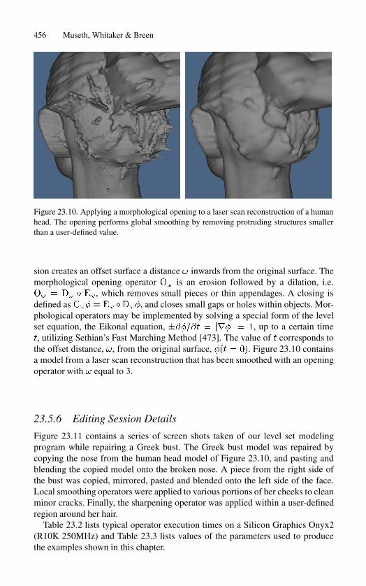
Figure 23.10. Applying a morphological opening to a laser scan reconstruction of a humanhead. The opening performs global smoothing by removing protruding structures smallerthan a user-defined value.

sion creates an offset surface a distance � inwards from the original surface. Themorphological opening operator �� is an erosion followed by a dilation, i.e.�� Æ ��, which removes small pieces or thin appendages. A closing isdefined as �� Æ��, and closes small gaps or holes within objects. Mor-phological operators may be implemented by solving a special form of the levelset equation, the Eikonal equation, �� , up to a certain time�, utilizing Sethian’s Fast Marching Method [473]. The value of � corresponds tothe offset distance, �, from the original surface, �� . Figure 23.10 containsa model from a laser scan reconstruction that has been smoothed with an openingoperator with � equal to 3.

23.5.6 Editing Session Details

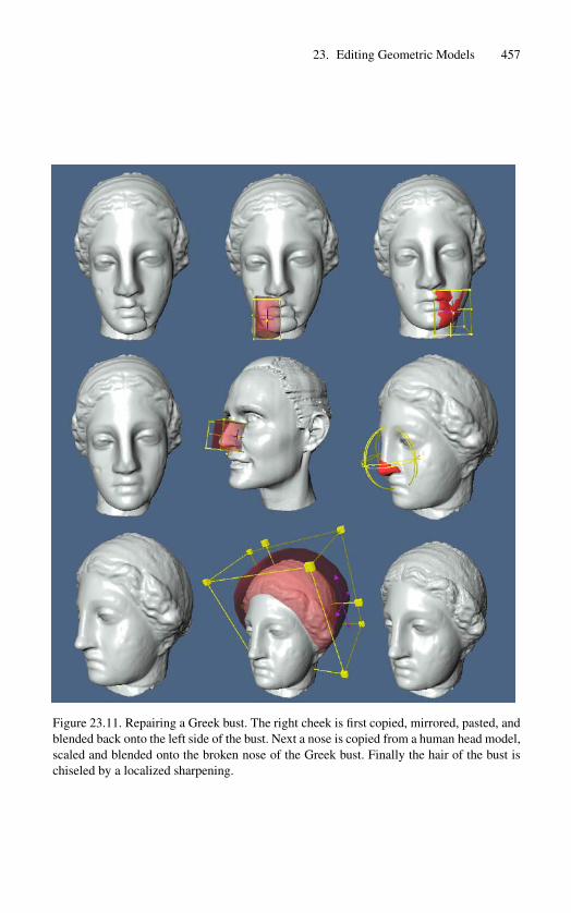
Figure 23.11 contains a series of screen shots taken of our level set modelingprogram while repairing a Greek bust. The Greek bust model was repaired bycopying the nose from the human head model of Figure 23.10, and pasting andblending the copied model onto the broken nose. A piece from the right side ofthe bust was copied, mirrored, pasted and blended onto the left side of the face.Local smoothing operators were applied to various portions of her cheeks to cleanminor cracks. Finally, the sharpening operator was applied within a user-definedregion around her hair.

Table 23.2 lists typical operator execution times on a Silicon Graphics Onyx2(R10K 250MHz) and Table 23.3 lists values of the parameters used to producethe examples shown in this chapter.


Figure 23.11. Repairing a Greek bust. The right cheek is first copied, mirrored, pasted, andblended back onto the left side of the bust. Next a nose is copied from a human head model,scaled and blended onto the broken nose of the Greek bust. Finally the hair of the bust ischiseled by a localized sharpening.


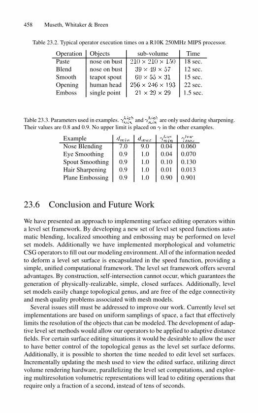
Table 23.2. Typical operator execution times on a R10K 250MHz MIPS processor.

Operation Objects sub-volume TimePaste nose on bust �� 18 sec.Blend nose on bust �� 12 sec.Smooth teapot spout �� 15 sec.Opening human head �� 22 sec.Emboss single point �� 1.5 sec.

Table 23.3. Parameters used in examples. �� and �� are only used during sharpening.Their values are 0.8 and 0.9. No upper limit is placed on � in the other examples.

Example ��

��

Nose Blending 7.0 9.0 0.04 0.060Eye Smoothing 0.9 1.0 0.04 0.070Spout Smoothing 0.9 1.0 0.10 0.130Hair Sharpening 0.9 1.0 0.01 0.013Plane Embossing 0.9 1.0 0.90 0.901

23.6 Conclusion and Future Work

We have presented an approach to implementing surface editing operators withina level set framework. By developing a new set of level set speed functions auto-matic blending, localized smoothing and embossing may be performed on levelset models. Additionally we have implemented morphological and volumetricCSG operators to fill out our modeling environment. All of the information neededto deform a level set surface is encapsulated in the speed function, providing asimple, unified computational framework. The level set framework offers severaladvantages. By construction, self-intersection cannot occur, which guarantees thegeneration of physically-realizable, simple, closed surfaces. Additionally, levelset models easily change topological genus, and are free of the edge connectivityand mesh quality problems associated with mesh models.

Several issues still must be addressed to improve our work. Currently level setimplementations are based on uniform samplings of space, a fact that effectivelylimits the resolution of the objects that can be modeled. The development of adap-tive level set methods would allow our operators to be applied to adaptive distancefields. For certain surface editing situations it would be desirable to allow the userto have better control of the topological genus as the level set surface deforms.Additionally, it is possible to shorten the time needed to edit level set surfaces.Incrementally updating the mesh used to view the edited surface, utilizing directvolume rendering hardware, parallelizing the level set computations, and explor-ing multiresolution volumetric representations will lead to editing operations thatrequire only a fraction of a second, instead of tens of seconds.


We have presented five example level set surface editing operators. Given thegenerality and flexibility of our framework many more can be developed. Weintend to explore operators that utilize Gaussian and principal curvature, extendembossing to work directly with lines, curves and solid objects, and ones thatmay be utilized for general surface manipulations, such as dragging, warping,and sweeping.

Acknowledgements

We would like to thank Sean Mauch for his scan conversion programs, Jasonwood for his useful visualization tools, Al Barr and Mathieu Desbrun for theirhelpful suggestions, and Katrine Museth for helping us with one of the figures.The Greek bust and human head models were provided by Cyberware Inc. Theteapot model was provided by the University of Utah’s Geometric Design andComputation Group. This work was financially supported by National ScienceFoundation grants ASC-89-20219, ACI-9982273 and ACI-0083287.

23.7 Appendix: Curvature of Level Set Surfaces

The principle curvatures and principle directions are the eigenvalues and eigen-vectors of the shape matrix [164]. For an implicit surface, the shape matrix is thederivative of the normalized gradient (surface normals) projected onto the tangentplane of the surface. If we let the normals be � � ��, the derivative of thisis the �� matrix

� �

��

��

��

��

��

��

�� (23.11)

The projection of this derivative matrix onto the tangent plane gives the shapematrix [164] � � � �� , where � is the exterior product. The eigen-values of the matrix� are �� and zero, and the eigenvectors are the principledirections and the normal, respectively. Because the third eigenvalue is zero, wecan compute �� and various differential invariants directly from the invariantsof�. Thus the weighted curvature flow is computing from� using the identities � ��, � � ��, and � � �� . The choice of numericalmethods for computing � is discussed in the following section. The principlecurvature are calculated by solving the quadratic

��

��

�� (23.12)

In many circumstances, the curvature term, which is a kind of directionaldiffusion, which does not suffer from overshooting, can be computed directlyfrom first- and second-order derivatives of � using central difference schemes.


n[p-1,q] n[p,q]

n[p,q-1]

n[p,q]

p-1 p p+1

q-1

q

q+1

N computed asdifference of normals atoriginal grid location

Staggered normalscomputed using 6neighbors (18 in 3D)

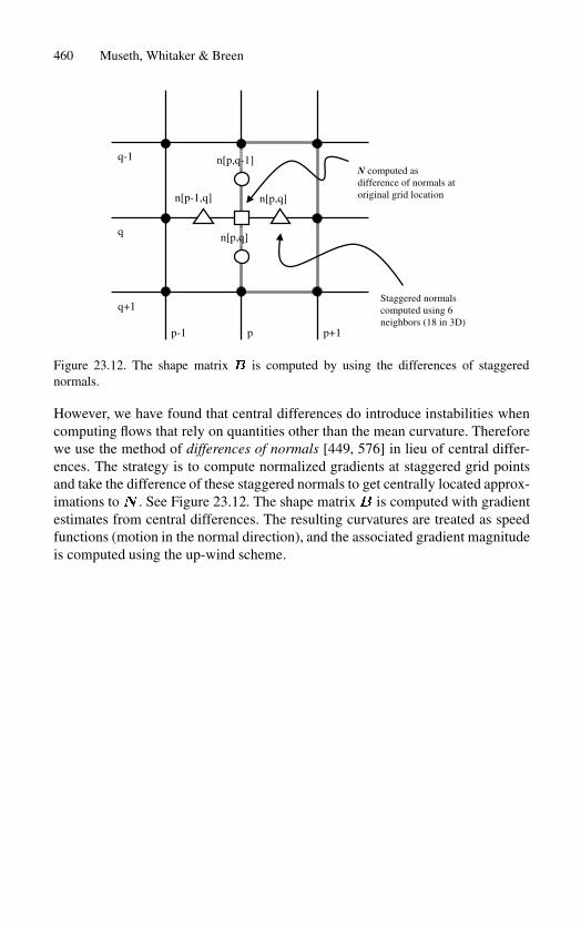
Figure 23.12. The shape matrix � is computed by using the differences of staggerednormals.

However, we have found that central differences do introduce instabilities whencomputing flows that rely on quantities other than the mean curvature. Thereforewe use the method of differences of normals [449, 576] in lieu of central differ-ences. The strategy is to compute normalized gradients at staggered grid pointsand take the difference of these staggered normals to get centrally located approx-imations to� . See Figure 23.12. The shape matrix� is computed with gradientestimates from central differences. The resulting curvatures are treated as speedfunctions (motion in the normal direction), and the associated gradient magnitudeis computed using the up-wind scheme.

Documents

Geometric Level Set Methods in Imaging, Vision, and Graphics || Editing Geometric Models