Embed Size (px)
Citation preview
MOX-Report No. 41/2015
Geometric multiscale modeling of the cardiovascularsystem, between theory and practice
Quarteroni, A.; Veneziani, A.; Vergara, C.
MOX, Dipartimento di Matematica Politecnico di Milano, Via Bonardi 9 - 20133 Milano (Italy)
[email protected] http://mox.polimi.it
Geometric multiscale modeling of the cardiovascular
system, between theory and practice
A. Quarteroni1, A. Veneziani2, C. Vergara3
September 26, 2015
1 Chair of Modelling and Scientific Computing, Ecole Polytechnique Federale de
Lausanne, Switzerland, [email protected] Department of Mathematics and Computer Science, Emory University, Atlanta, GA,
USA, [email protected] MOX, Dipartimento di Matematica, Politecnico di Milano, Italy,
Keywords: Blood flow simulation, fluid-structure interaction, 1D models, lumpedparameter models, geometric multiscale coupling
Abstract
This review paper addresses the so called geometric multiscale approachfor the numerical simulation of blood flow problems, from its origin (that wecan collocate in the second half of ’90s) to our days. By this approach theblood fluid-dynamics in the whole circulatory system is described math-ematically by means of heterogeneous featuring different degree of detailand different geometric dimension that interact together through appropri-ate interface coupling conditions.
Our review starts with the introduction of the stand-alone problems,namely the 3D fluid-structure interaction problem, its reduced representa-tion by means of 1D models, and the so-called lumped parameters (aka 0D)models, where only the dependence on time survives. We then address spe-cific methods for stand-alone 3D models when the available boundary dataare not enough to ensure the mathematical well posedness. These so-called“defective problems” naturally arise in practical applications of clinical rel-evance but also because of the interface coupling of heterogeneous problemsthat are generated by the geometric multiscale process. We also describespecific issues related to the boundary treatment of reduced models, par-ticularly relevant to the geometric multiscale coupling. Next, we detail themost popular numerical algorithms for the solution of the coupled problems.Finally, we review some of the most representative works - from differentresearch groups - which addressed the geometric multiscale approach in thepast years.
1
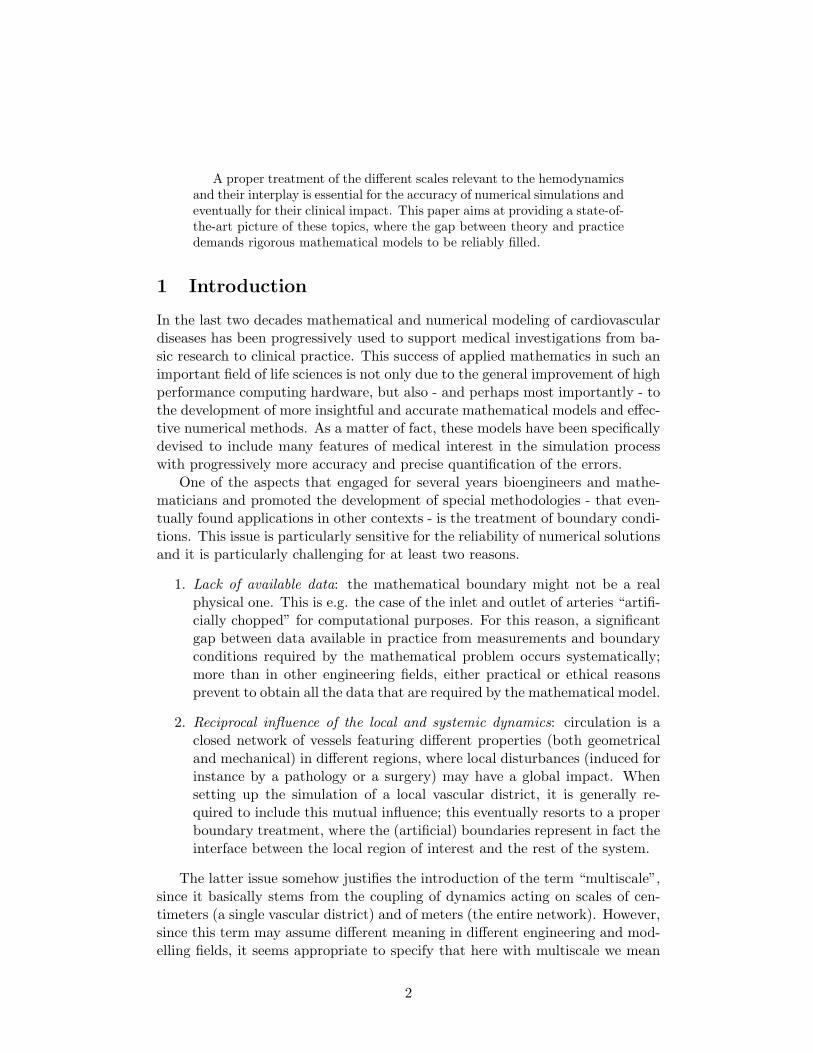
A proper treatment of the different scales relevant to the hemodynamicsand their interplay is essential for the accuracy of numerical simulations andeventually for their clinical impact. This paper aims at providing a state-of-the-art picture of these topics, where the gap between theory and practicedemands rigorous mathematical models to be reliably filled.
1 Introduction
In the last two decades mathematical and numerical modeling of cardiovasculardiseases has been progressively used to support medical investigations from ba-sic research to clinical practice. This success of applied mathematics in such animportant field of life sciences is not only due to the general improvement of highperformance computing hardware, but also - and perhaps most importantly - tothe development of more insightful and accurate mathematical models and effec-tive numerical methods. As a matter of fact, these models have been specificallydevised to include many features of medical interest in the simulation processwith progressively more accuracy and precise quantification of the errors.
One of the aspects that engaged for several years bioengineers and mathe-maticians and promoted the development of special methodologies - that even-tually found applications in other contexts - is the treatment of boundary condi-tions. This issue is particularly sensitive for the reliability of numerical solutionsand it is particularly challenging for at least two reasons.
1. Lack of available data: the mathematical boundary might not be a realphysical one. This is e.g. the case of the inlet and outlet of arteries “artifi-cially chopped” for computational purposes. For this reason, a significantgap between data available in practice from measurements and boundaryconditions required by the mathematical problem occurs systematically;more than in other engineering fields, either practical or ethical reasonsprevent to obtain all the data that are required by the mathematical model.
2. Reciprocal influence of the local and systemic dynamics: circulation is aclosed network of vessels featuring different properties (both geometricaland mechanical) in different regions, where local disturbances (induced forinstance by a pathology or a surgery) may have a global impact. Whensetting up the simulation of a local vascular district, it is generally re-quired to include this mutual influence; this eventually resorts to a properboundary treatment, where the (artificial) boundaries represent in fact theinterface between the local region of interest and the rest of the system.
The latter issue somehow justifies the introduction of the term “multiscale”,since it basically stems from the coupling of dynamics acting on scales of cen-timeters (a single vascular district) and of meters (the entire network). However,since this term may assume different meaning in different engineering and mod-elling fields, it seems appropriate to specify that here with multiscale we mean
2
the coupling of different length scales, so that we will use this term in com-bination with the adjective “geometric”. While a local detailed hemodynamicanalysis requires in general the accurate solution of fluid-structure interactionproblems (blood and vascular walls), henceforth in the true 3D domain, quan-titative investigations of the cardiovascular system have often been based onsurrogate models featuring lower geometric dimensions. We recall the pioneer-ing work by Otto Frank [70], followed up by the simulators of Nico Westerhof[205], based on the analogy of the circulatory network with electrical circuits.These are lumped parameter or - with a popular notation that follows from dis-carding an explicit dependence on any space dimension and that will be usedextensively later on - 0D models. Even earlier (two centuries!) L. Euler proposedhis equations for describing the motion of a fluid in elastic pipes, having in mindblood flow in arteries [53]. This system of equations has then provided the base-line for assembling mathematical models of several arterial segments, in eachof them the axial dynamics is the only one retained, resorting to what we willdenote as 1D models. Because of their hyperbolic nature, these models turnedout to be particularly effective in capturing the pressure wave propagation alongthe arterial tree.
The two issues listed above turn out to be strictly related. In order to addresspoint 2 above bioengineers looked for reliable boundary conditions for a districtof interest by solving Westerhof-like 0D models to be prescribed in a specificdistrict. Then, to solve the incompressible Navier-Stokes equations in that dis-trict, this naturally brought up the problem of defective data set, as for point 1.For example, a lumped parameter as well as 1D model can provide a flow rateincoming a district of interest. However a Navier-Stokes solver for that districtrequires the whole velocity field at the boundaries. A practical and popular ap-proach consists in conjecturing an a priori velocity profile (typically a parabolicone) to be fitted with the flow rate available from the systemic model. Similarconsiderations hold for Neumann-like conditions such as those prescribing thetraction or the pressure. However, the accuracy of these heuristic approachesmay be sometimes questionable. A more sound mathematical approach wasdeemed in order to enhance both reliability and accuracy. Starting from thesecond half of 90’s with the paper [165], this problem challenged several groupsand led to many different ideas.
The purpose of this work is to critically review these topics in order tohighlight the important impact that mathematically sound methods may haveon the accuracy of the results. Nevertheless, we will include in our discussionalso practical aspects that need to be considered when performing geometricmultiscale simulations on real problems.
Moving from a brief description (Sect. 2) of the different models that can beused in a stand-alone fashion to describe the circulation with a different level ofdetail (3D, 1D or 0D), we consider more specifically the issues related to theirboundary treatment in Sect. 3. While for the 3D problem we need to considerhow to fill the gap between insufficient available data and a complete data set,
3
for 1D problems the treatment of the boundary requires special techniques toavoid numerical artifacts in computing the pressure wave propagation. Finally,for 0D models the concept of “boundary” is actually inappropriate, since themodel reduction drops the explicit space dependence. However, in view of cou-pling dimensionally heterogeneous models, we need to address how data at theinterface of the lumped parameter compartment can be spatially localized. InSect. 4 we address extensively the coupling of the different models that leads to a“geometric multiscale“ description, whereas we will address different approachesfor the numerical solution of the dimensionally heterogeneous problems in Sect.5. In Sect. 6 we provide an annotated review of selected works to outline signif-icant contributions of the literature over the last two decades. Conclusions andperspectives follow in Sect. 7.
2 Stand-alone models: fluid, structure and their in-
teraction
In this section, we start from the classical 3D model for fluid-structure interactionin hemodynamics. We then address the 1D and finally 0D models. Each of thesemodels is standing alone; the analysis of coupling will make the subject of nextsections. We necessarily limit to a brief introduction to this vast and still activefield of research.
2.1 The 3D model
2.1.1 Modeling blood, vascular wall and their interaction
We start considering a 3D high fidelity description of blood flowing in a vesselof interest, the vascular wall deformation, and their interaction (fluid-structureinteraction - FSI).
It is worth mentioning that many vascular diseases affect large and mediumsized arteries. In such districts, blood is modeled by means of the Navier-Stokes(NS) equations for incompressible homogeneous Newtonian fluids [149, 184, 185,64]. Effects related to non-Newtonian rheology such as the ones induced bypathologies (for instance the sickle cell disease) or in the capillaries need to bespecifically addressed and are not considered in the present work. We refer theinterested reader to, e.g., [171].
As for the structure problem, we assume the arterial wall to obey a (possiblynonlinear) finite elastic law relating stress to strain in the arterial tissue. This isclearly a simplification of the indeed far more complex behavior of arterial walls[90, 91] that however we postulate for the sake of simplicity. In more realisticsettings, strain is function of the stress but also of the loading history [72].
For the mathematical formulation of the problem, we find convenient towrite the fluid equations with respect to an Eulerian frame of reference, and wedenote by Ωf ⊂ R
3 the time-varying arterial lumen (see Figure 1, left), while
4
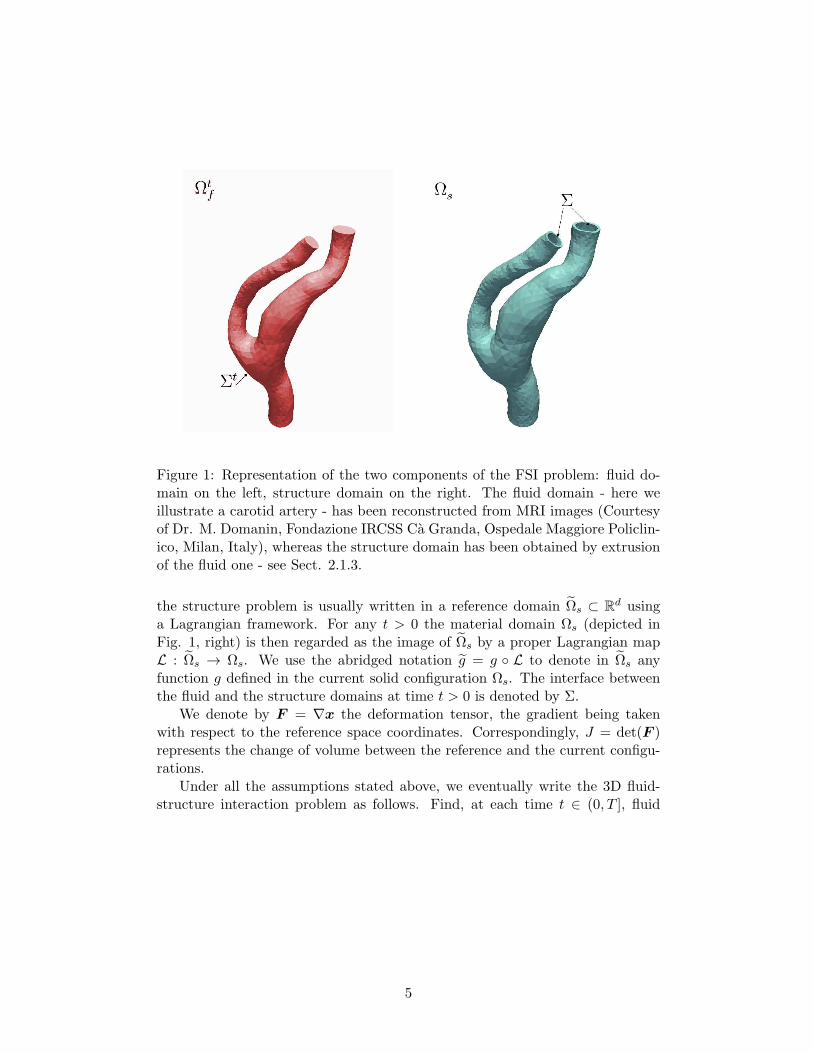
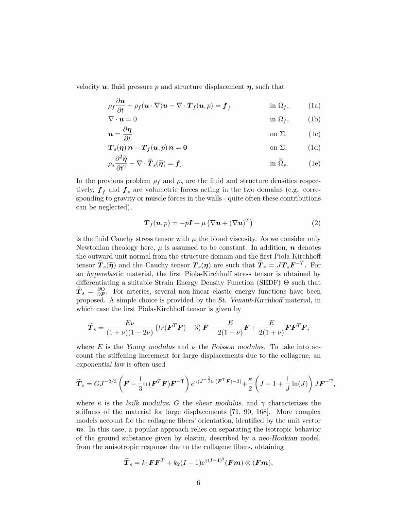
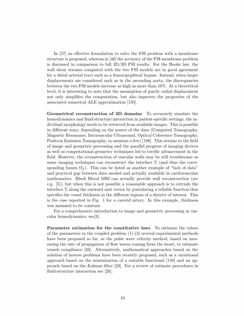
Figure 1: Representation of the two components of the FSI problem: fluid do-main on the left, structure domain on the right. The fluid domain - here weillustrate a carotid artery - has been reconstructed from MRI images (Courtesyof Dr. M. Domanin, Fondazione IRCSS Ca Granda, Ospedale Maggiore Policlin-ico, Milan, Italy), whereas the structure domain has been obtained by extrusionof the fluid one - see Sect. 2.1.3.
the structure problem is usually written in a reference domain Ωs ⊂ Rd using
a Lagrangian framework. For any t > 0 the material domain Ωs (depicted inFig. 1, right) is then regarded as the image of Ωs by a proper Lagrangian mapL : Ωs → Ωs. We use the abridged notation g = g L to denote in Ωs anyfunction g defined in the current solid configuration Ωs. The interface betweenthe fluid and the structure domains at time t > 0 is denoted by Σ.
We denote by F = ∇x the deformation tensor, the gradient being takenwith respect to the reference space coordinates. Correspondingly, J = det(F )represents the change of volume between the reference and the current configu-rations.
Under all the assumptions stated above, we eventually write the 3D fluid-structure interaction problem as follows. Find, at each time t ∈ (0, T ], fluid
5
velocity u, fluid pressure p and structure displacement η, such that
ρf∂u
∂t+ ρf (u · ∇)u−∇ · T f (u, p) = ff in Ωf , (1a)
∇ · u = 0 in Ωf , (1b)
u =∂η
∂ton Σ, (1c)
T s(η)n− T f (u, p)n = 0 on Σ, (1d)
ρs∂2η
∂t2−∇ · T s(η) = f s in Ωs. (1e)
In the previous problem ρf and ρs are the fluid and structure densities respec-tively, ff and f s are volumetric forces acting in the two domains (e.g. corre-sponding to gravity or muscle forces in the walls - quite often these contributionscan be neglected),
T f (u, p) = −pI + µ(∇u+ (∇u)T
)(2)
is the fluid Cauchy stress tensor with µ the blood viscosity. As we consider onlyNewtonian rheology here, µ is assumed to be constant. In addition, n denotesthe outward unit normal from the structure domain and the first Piola-Kirchhofftensor T s(η) and the Cauchy tensor T s(η) are such that T s = JT sF
−T . Foran hyperelastic material, the first Piola-Kirchhoff stress tensor is obtained bydifferentiating a suitable Strain Energy Density Function (SEDF) Θ such thatT s = ∂Θ
∂F . For arteries, several non-linear elastic energy functions have beenproposed. A simple choice is provided by the St. Venant-Kirchhoff material, inwhich case the first Piola-Kirchhoff tensor is given by
T s =Eν
(1 + ν)(1− 2ν)
(tr(F TF )− 3
)F − E
2(1 + ν)F +
E
2(1 + ν)FF TF ,
where E is the Young modulus and ν the Poisson modulus. To take into ac-count the stiffening increment for large displacements due to the collagene, anexponential law is often used
T s = GJ−2/3
(F − 1
3tr(F TF )F−T
)eγ(J
−
23 tr(F TF )−3)+
κ
2
(J − 1 +
1
Jln(J)
)JF−T,
where κ is the bulk modulus, G the shear modulus, and γ characterizes thestiffness of the material for large displacements [71, 90, 168]. More complexmodels account for the collagene fibers’ orientation, identified by the unit vectorm. In this case, a popular approach relies on separating the isotropic behaviorof the ground substance given by elastin, described by a neo-Hookian model,from the anisotropic response due to the collagene fibers, obtaining
T s = k1FF T + k2(I − 1)eγ(I−1)2(Fm)⊗ (Fm),
6
with I = m · (F TF m) being an invariant of the system and k1, k2 suitablematerial parameters [91]. More complete laws also account for the symmetricalhelical arrangement of the collagene fibers, with directionsm andm′ lying in thetangential plane of the artery [91]. The arterial tissue is sometimes considered asincompressible [38]. In this case, one has to enforce the constraint J = 1 and inthe related Cauchy stress tensor the term −psI is added, ps being the hydrostaticpressure (which plays the role of Lagrange multiplier of the incompressibilityconstraint).
The matching conditions enforced at the FS interface follow from the con-tinuity of velocities (kinematic condition) (1c) and the continuity of tractions(dynamic condition) (1d).
Finally, problem (1) is completed by boundary conditions at ∂Ωf \ Σ and
∂Ωs\Σ, and by initial conditions on u,η and∂η
∂t. Boundary conditions typically
prescribe:
- for the fluid subproblem, the upstream velocity uup on the proximal boundariesand absorbing traction conditions T f · n = h on the distal boundaries, h beinga suitable function [136];
- for the structure subproblem, either η = 0 (fixed boundary) or η · n = 0together with (T s · n) · τ = 0, τ being the unit tangential directions (displace-ment allowed in the tangential direction).
Other conditions may be prescribed if patient-specific measured data are avail-able. However - as pointed out in the Introduction - measures seldom providea complete data set to be used in the computation and a preprocessing step isrequired as we will illustrate in Sect. 3.
Boundary conditions at the external lateral boundary of the structure ac-count for the effect of the tissues surrounding the artery. In [126], an algebraiclaw is proposed to mimic an elastic behavior of this tissue. This law is meant atrepresenting the action of these tissues by independent springs characterized byan elastic space dependent coefficient αST (ST stands for “surrounding tissues”).This yields the following Robin boundary condition
αST η + T s(η) n = Pextn, on Σext, (3)
where Σext is the external lateral surface and Pext the external pressure. Fortuning αST , we refer the reader to [112, 43].
Under several regularity assumptions, these data may guarantee well posed-ness to the coupled fluid-structure problem, see e.g. [19, 77, 32, 113] for acomprehensive description of this topic.
7
2.1.2 Numerical discretization
Numerical approximation of (1) demands an appropriate discretization of timeas well as space variables. One of the challenging aspects here is the movementof the domain, both for the fluid and the solid. For the structure, deformationsare in general small enough so that a purely Lagrangian description is a viableoption. On the contrary, for the fluid we need to use a Lagrangian description ofthe fluid-structure interface and an Eulerian description of the proximal/distalboundaries. As pointed out in the Introduction, these are artificial portions ofthe boundary and their location does not follow the fluid displacement. Thishybrid situation led to the introduction of the so-called Arbitrary Lagrangian-
Eulerian (ALE) formulation [93, 51]. With this approach the displacement fieldat the boundary is arbitrarily extended into the domain. For instance, a har-monic lifting (i.e. the displacement computed by solving a Laplace problem)is a popular choice. This provides a convenient yet non-inertial frame of ref-erence where to write the Navier-Stokes equations (ALE formulation). In thisframework, the solution of the fluid and structure problem is supplemented bythe solution of the lifting (hereafter called “geometric coupling problem”). Dif-ferent methods can be used for the solution of the FSI plus geometric couplingproblem. Time discretization can be obtained by standard finite difference pro-cedures. Among the others, we mention Backward Difference Formulas (BDF),successfully adopted for both fluid and structure problems. Alternatively, theϑ−method for fluid and Newmark schemes for the structure are successfully usede.g. in [133]. For the space discretization, finite elements and finite volumes arethe most popular strategies. Notice however that the movement of the domainmakes the accuracy analysis of the overall procedure quite challenging as theinterplay between space and time accuracy of the discretization of the fluid,structure and geometric coupling problems is not trivial.
At the algorithmic level, after a suitable treatment of the geometric coupling(either implicit applying, e.g., the Newton method [134] or explicit by means ofextrapolation from previous time steps [55]), the FSI problem may be solved bymonolithic as well as segregated approaches. In the former case, the completenon-linear system arising after the space discretization is assembled and solvedwith a suitable preconditioned Krylov [86, 15], domain-decomposition [44, 50]or multigrid [75, 13] methods. In the partitioned case the successive solutionof the fluid and solid subproblems in an iterative framework is carried out (see,e.g., [39, 55, 11, 46, 9, 105, 134]). In this case, the schemes feature in generalpoor convergence properties due to the added mass effect, that predicts a break-down of performances when the values of the densities of fluid and structureare close as it happens in hemodynamics [39, 69, 10, 76, 137]. Alternatively, onecould consider space-time finite elements, see, e.g., [187, 17], or the iso-geometricanalysis, see [15].
It is worth noting that for problems related to the movement of structuresfloating in incompressible fluids, a successful approach is the so-called Immersed
8
Boundary Method originated by the work of C. Peskin [153, 34].Recent introductions to the numerical approximation of FSI problems can
be found in [54] (2009) and [18] (2013).
2.1.3 Further developments and comments
Modeling the structure as a 2D membrane For the sake of simplification,the structure may be modelled as a 2D membrane whose position in space atany time exactly coincides with the FS interface Σ. In this case, only the radialdisplacement ηr is considered, and a possible mathematical representation isgiven by the generalized string model [163]:
ρsHs∂2ηr∂t2
−∇ · (P∇ηr) + βHsηr = fs at Σ, (4)
where the manifold Σ represents the reference membrane configuration, Hs thestructure thickness, tensor P accounts for shear deformations and, possibly,for prestress, β(x) = E
1−ν2 (4ρ21 − 2(1 − ν)ρ2), where ρ1(x) and ρ2(x) are the
mean and Gaussian curvatures of Σ, respectively, [136], and fs the forcing term.The previous model is derived from the equations of the linear infinitesimalelasticity (Hooke law) under the assumptions of small thickness, plane stresses,and negligible elastic bending terms. To account for the effect of the surroundingtissue, the term β in (4) needs to be properly modified. For example, in the caseof an elastic tissue as in (3), we need to substitute β with β = β + αST , withαST the elastic coefficient of the tissue.
In the particular case where Σ is the lateral surface of a cylinder and anydependence on the circumferential coordinate is discarded, model (4) reduces to
ρsHs∂2ηr∂t2
− kGHs∂2ηr∂z2
+EHs
(1− ν2)R20
Hsηr = fs at Σ, (5)
k being the Timoshenko correction factor, G the shear modulus, R0 the cylinderradius, and z the axial coordinate. Often, in the latter case, also a visco-elastic
term of the form γv∂3ηr∂2z∂t
is added, with γv a suitable visco-elastic parameter[163].
When (4) is coupled with the fluid equations (1a)-(1b), possible matchingconditions read
u · n =∂ηr∂t
at Σ,
T f (u, p)n · n = fs at Σ.
In fact, the coupling occurs only in the radial direction, so that we have tocomplete the conditions at Σ for the fluid problem by prescribing tangentialinformation, e.g., homogeneous Dirichlet or Neumann data.
9
In [57] an effective formulation to solve the FSI problem with a membranestructure is proposed, whereas in [40] the accuracy of the FSI-membrane problemis discussed in comparison to full 3D/3D FSI results. For the Hooke law, thewall shear stresses computed with the two FSI models are in good agreementfor a distal arterial tract such as a femoropopliteal bypass. Instead, when largerdisplacements are considered such as in the ascending aorta, the discrepanciesbetween the two FSI models increase as high as more than 10%. At a theoreticallevel, it is interesting to note that the assumption of purely radial displacementnot only simplifies the computation, but also improves the properties of theassociated numerical ALE approximation [135].
Geometrical reconstruction of 3D domains To accurately simulate thehemodynamics and fluid-structure interaction in patient-specific settings, the in-dividual morphology needs to be retrieved from available images. This is possiblein different ways, depending on the source of the data (Computed Tomography,Magnetic Resonance, Intravascular Ultrasound, Optical Coherence Tomography,Positron Emission Tomography, to mention a few) [186]. This attains to the fieldof image and geometric processing and the parallel progress of imaging devicesas well as computational geometry techniques led to terrific advancement in thefield. However, the reconstruction of vascular walls may be still troublesome assome imaging techniques can reconstruct the interface Σ (and thus the corre-sponding lumen Ωf ). This can be listed as another example of “lack of data”and practical gap between data needed and actually available in cardiovascularmathematics. Black Blood MRI can actually provide wall reconstruction (seee.g. [5]), but when this is not possible a reasonable approach is to extrude theinterface Σ along the outward unit vector by postulating a reliable function thatspecifies the vessel thickness in the different regions of a district of interest. Thisis the case reported in Fig. 1 for a carotid artery. In this example, thicknesswas assumed to be constant.
For a comprehensive introduction to image and geometric processing in vas-cular hemodynamics, see[3].
Parameter estimation for the constitutive laws To estimate the valuesof the parameters in the coupled problem (1)-(3) several experimental methodshave been proposed so far, as the pulse wave velocity method, based on mea-suring the rate of propagation of flow waves coming form the heart, to estimatevessels compliance [33]. Alternatively, mathematical approaches based on thesolution of inverse problems have been recently proposed, such as a variational
approach based on the minimization of a suitable functional [148] and an ap-proach based on the Kalman filter [23]. For a review of estimate procedures influid-structure interaction see [20].
10
2.2 The 1D model
Numerical modeling of the whole cardiovascular system by means of 3D models iscurrently out of reach because of the complexity of the computational domain,that would require the acquisition and reconstruction of thousands (or evenmore) vessels. This would lead to huge algebraic linear systems to be solved ateach time step, not affordable also for modern supercomputers, at least not forclinical applications going beyond prototypes and proofs of concept.
On the other hand, in many applications the level of information of 3Dmodels exceeds the accuracy requested, in particular when we aim at modelingthe dynamics occurring at the systemic more than at a local level. In this caseit is preferable to adopt reduced models for which the computational efficiencyand the systemic breath are considered more important than the local accuracy.One-dimensional (1D) models for the description of blood flow in a compliantvessel where the only space coordinate is the one associated with the vessel axismay provide a good trade-off among the different requirements. They have beenintroduced almost 250 years ago by L. Euler [53], and then rediscovered in thesecond half of the XX century in [14] - see also [94, 95]. The construction ofthese models is the result of two steps.
1. The description of motion of an incompressible fluid in a single compliantpipe. Only the axial dynamics is included; several simplifying assump-tions are postulated - as we see later on - to apply conservation of massand momentum along one space dimension. A suitable constitutive law isintroduced to describe the relation between pressure and area of the pipeto include the arterial compliance;
2. The coupling of different segments composing the arterial tree by writ-ing appropriate interface conditions between the single-segment modelsobtained at the previous step.
These reduced models do not allow to describe secondary flows. However,they provide average quantities at a very low computational time, a desirablefeature that has been exploited since the ’80s (see, e.g., [7, 103, 88]). It is worthreminding the book [145] reporting accurate investigations of the circulatorysystems by means of Euler-like models.
Let us detail hereafter steps 1 and 2.
2.2.1 The Euler model for an arterial segment
One dimensional models may be derived in different ways. One of the mostpopular (and more sound from a physical standpoint) moves from the full 3Dmodel and several simplifying assumptions on the behavior of the flow, the struc-ture and their interaction. Hereby, we briefly sketch these assumptions and theconsequent modeling procedure. Ample details can be found, e.g., in [160] and[146].
11
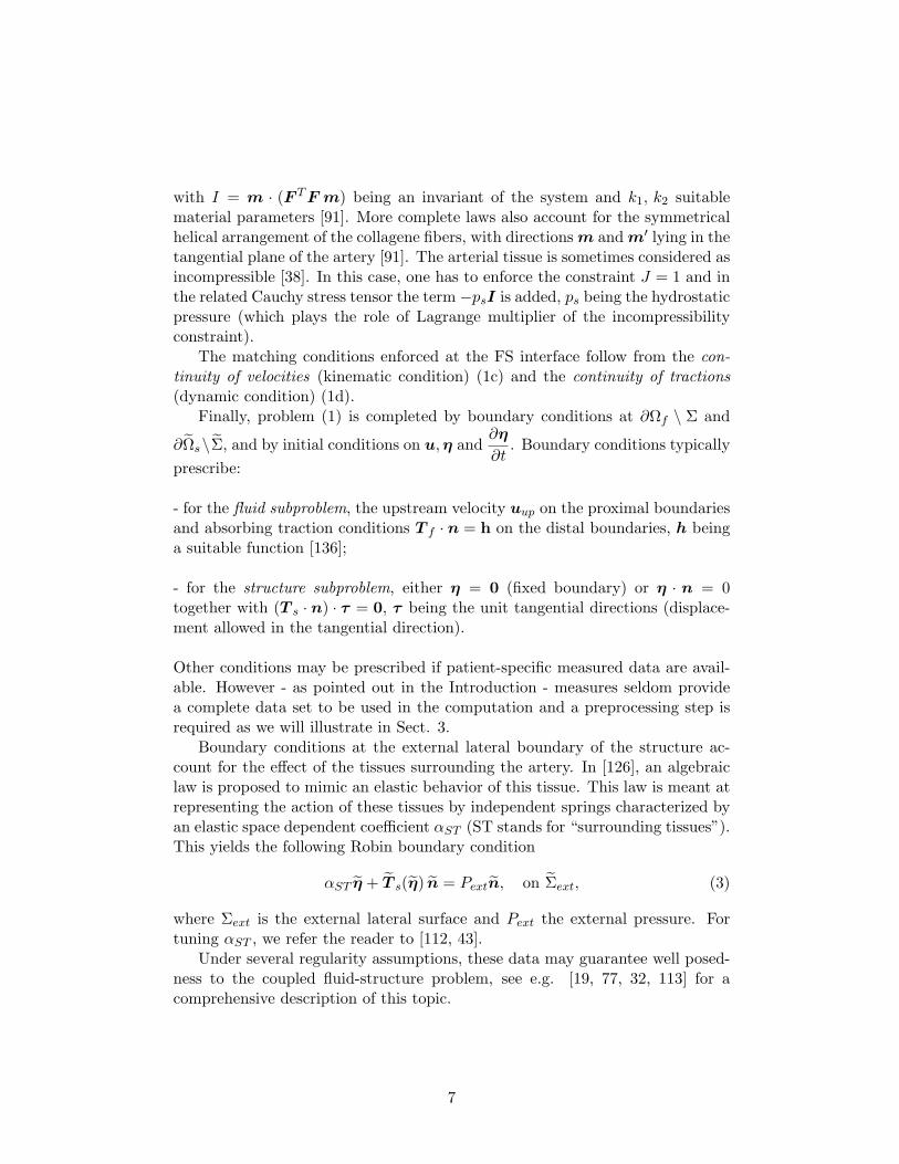
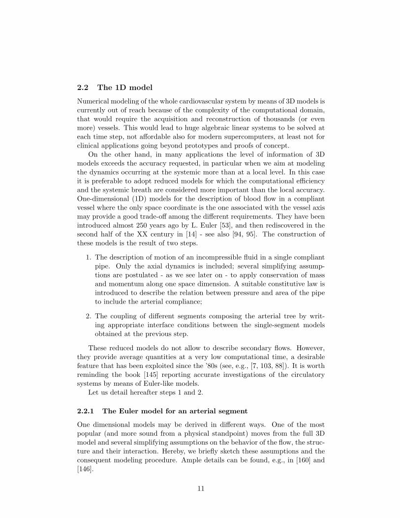
We assume the fluid domain to be represented by a cylindrical geometry ormore generally by a truncated cone. We refer for notations to Figure 2, wherea cylindrical coordinate system (r, ϕ, z) is outlined. We make the followingsimplifying assumptions: (i) the axis of the cylinder is fixed; (ii) for any z,the cross section S(t, z) is a circle (i.e. no dependence on the circumferentialcoordinate ϕ is assumed) with radius R(t, z); (iii) the solution of both fluid andstructure problems does not depend on ϕ; (iv) the pressure is constant over eachsection S(t, z); (v) the axial fluid velocity uz is dominant vs the other velocitycomponents; (vi) only radial displacements are allowed, so that the structuredeformation takes the form η = ηer, where er is the unit vector in the radialdirection; more precisely, we set η(t, z) = R(t, z) − R0(z) where R0(z) is thereference radius at the equilibrium; (vii) the viscous effects are modeled by alinear term proportional to the flow rate; (viii) the vessel structure is modeledas a membrane with constant thickness. As for assumption (vii), this is justifiedby the well known Poiseuille solution for a 3D Newtonian incompressible fluidin a circular cylinder, where the effects of viscosity are actually proportional tothe flow rate.
xz
y
R(t, z)S(t, z)
ϕ
r
Figure 2: Fluid domain for the derivation of the 1D model.
To write the reduced model, we introduce the following quantities: A(t, z) =|S(t, z)| = πR(t, z)2 (lumen section area), u(t, z) = A−1
∫S(t,z) uz(t, z)dS (mean
velocity), s(r/R) is a velocity profile such that uz(t, r, z) = u(t, z)s (r/R(t, z)),Q(t, z) = ρf
∫S(t,z) uz dS = ρfA(t, z)u(t, z) (flow rate), P (t, z) = A−1
∫S(t,z) p(t, z) dS
(mean pressure).As for the structure and its interaction with the fluid, we need a closure
condition that states a functional dependence of the pressure on the lumen area(or equivalently on the displacement ηr) of the following form
P (t, z) = Pext + ψ(A(t, z), A0(z),β(z)), (6)
where ψ is a given function satisfying ∂ψ∂A > 0, ψ(A0) = 0 and Pext the external
pressure. Here β is a vector of parameters describing the mechanical propertiesof the membrane. The condition on ∂ψ
∂A responds to the intuitive expectationthat the area gets larger when the pressure increases.
12
By integrating over the sections S the momentum fluid equation (1a) in thez− direction and the mass conservation law (1b), we obtain the following system
∂U
∂t+H(U)
∂U
∂z+B(U) = 0 z ∈ (0, L), t > 0, (7)
where U = [A Q]T is the vector of the unknowns, α =
∫S u
2z
Au2=
1
A
∫ 1
0s2(y)dy
is the so called momentum flux correction coefficient (aka Coriolis coefficient),Kr = −2πµs′(1) is the friction parameter (due to the viscous nature of the fluid),
c1 =√
Aρf
∂ψ∂A , while
H(U) =
[0 1
c21 − α(QA
)22αQA
], (8a)
B(U) =
[0
KrQA + A
ρf
∂ψ∂A0
∂A0∂z + A
ρf
∂ψ∂β
∂β∂z
](8b)
represent the flux matrix and the dissipation vector term. A complete derivationof the model can be found e.g. in [145, 94], and [146].
Alternatively, one could introduce the conservative form of the 1D system,which reads
∂U
∂t+∂F (U)
∂z+ S(U) = 0 z ∈ (0, L), t > 0, (9)
where F = [Q αQ2/A + C1]T and S = B − [0 ∂C1
∂A0
dA0dz + ∂C1
∂βdβdz ]
T , with
C1 =∫ AA0c21.
For blood flow a classical choice of the velocity profile is s(y) = γ−1(γ +2)(1 − yγ). For γ = 1 we have α = 1 (flat profile), for γ = 2 we have α = 4/3(parabolic profile). Accordingly, we have Kr = 2πµ(γ+2)(= 8πµ for a parabolicprofile). Other, more sophisticated choices can be operated. For instance in [8]the pulsatile Womersley profile - that is, the unsteady periodic counterpart ofthe Poiseuille solution for the Navier-Stokes problem in a cylinder - is accountedfor, while in [24] an approximated velocity profile is generated at each time stepby solving simplified equations near the wall and in the core of the vessel.
The term ∂A0∂z in B is typically non-positive, as it accounts for the so-called
vessel “tapering”, i.e. the fact that the area of the lumen reduces when pro-ceeding from proximal to distal direction. The term ∂β
∂z originates from possiblydifferent mechanical properties along the vessel, to describe, for example, thepresence of plaques or vascular prostheses. A special treatment of these termsobtained by regarding A0 and β as fictitious unknowns to be added to the sys-tem, is proposed in [128].
If A > 0, system (7) has two distinct real eigenvalues (see, e.g., [160])
λ1,2 = αu±√c21 + u2α(α− 1), (10)
13
hence it is strictly hyperbolic (see e.g. [111]). Under physiological conditions,c1 >> αu, yielding λ1 > 0 and λ2 < 0, thus we have two waves traveling inopposite directions.
A simple membrane law (6) can be obtained by (5) by dropping the shearand inertial terms, leading to the following algebraic relation [60, 65],
ψ(A,A0, β) = β
√A−
√A0
A0, with β =
√πHsE
1− ν2, (11)
where ν is the Poisson modulus of the membrane, E its Young modulus , and Hs
its thickness, yielding c1 =
√β√A
2ρfA0. This simple law, stating that the membrane
radial displacement ηr is linearly proportional to the fluid pressure, is successfullyconsidered in many applications, see, e.g., [181, 118, 80]. Other laws have beenproposed to account for other features of the arterial wall. For example thefollowing law stems from the generalized string model [163, 194]
ψ = m∂2A
∂t2− γ
∂A
∂t− a
∂2
∂z2
(√A−
√A0
)+ β
√A−
√A0
A0,
where m = ρsHs
2√πA0
is the mass of the membrane, γ a coefficient accounting for
visco-elastic effects and a for the longitudinal pre-stress [71]. This generatesthree differential extra-terms in the momentum equation that account for theinertial, visco-elastic and pre-stressed effects, respectively (see [60] for the ex-plicit expression of H and B in (7)). In [60] numerical results show that thewall-inertia term is important for large mass and/or high frequencies, the visco-elasticity term gives a small contribution, whereas the longitudinal pre-stressis important for strong area gradients (i.e. in presence of severe tapering orstenosis).
Different approaches have been introduced so far to account for visco-elasticeffects. For example, in [7] the author considers a dynamic Young modulus whichintroduces a phase difference between applied forces and resulting displacements.Non-linear elastic effects are described in [89, 169], by splitting the membranelaw in a non-linear elastic part and in a visco-elastic part. The first term is givenby a relation like (11) where however the parameter β depends non-linearly onthe pressure. As for the visco-elastic term, the authors consider the convolutionproduct between the elastic area and the derivative of a suitable creep function.The numerical results reported in [176, 169] show the importance of includingnon-linear terms and visco-elastic effects for the peripheral districts.
A more general membrane law is given by the following expression
ψ = β
((A
A0
)n1
−(A0
A
)n2), (12)
see [191]. For collapsible districts such as the veins, in [128] the authors pro-pose to use n1 = 10 and n2 = 3/2, which allows to properly describe the highcompliance of the veins. For a recent review on the 1D modelling of the venoussystem, see [190].
14
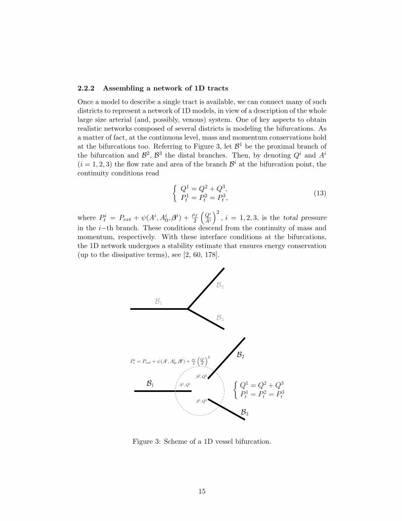
2.2.2 Assembling a network of 1D tracts
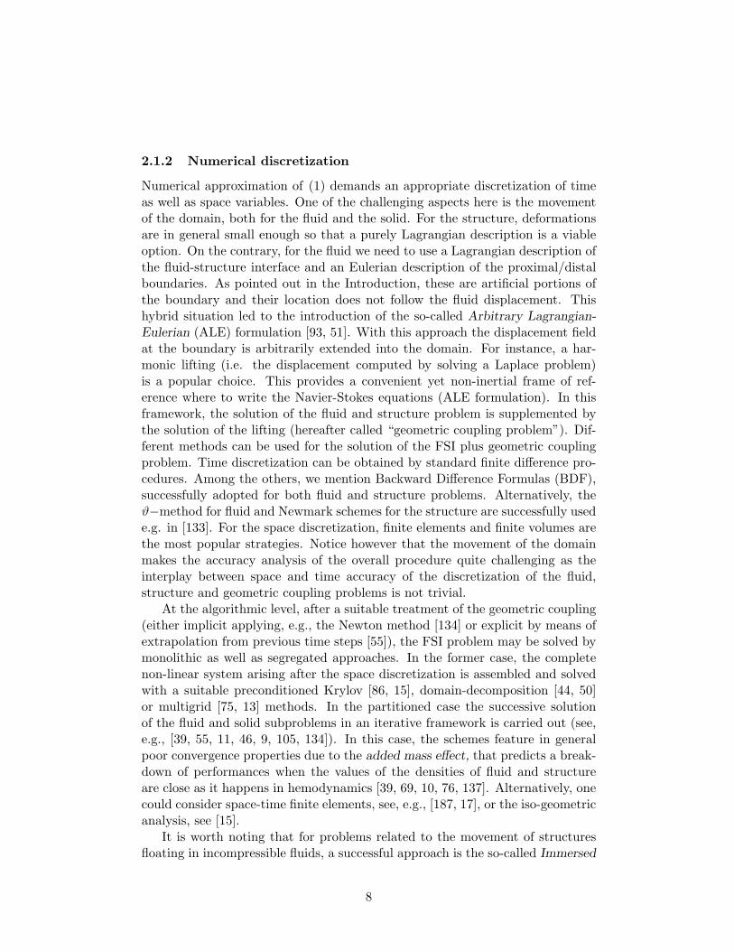
Once a model to describe a single tract is available, we can connect many of suchdistricts to represent a network of 1D models, in view of a description of the wholelarge size arterial (and, possibly, venous) system. One of key aspects to obtainrealistic networks composed of several districts is modeling the bifurcations. Asa matter of fact, at the continuous level, mass and momentum conservations holdat the bifurcations too. Referring to Figure 3, let B1 be the proximal branch ofthe bifurcation and B2, B3 the distal branches. Then, by denoting Qi and Ai
(i = 1, 2, 3) the flow rate and area of the branch Bi at the bifurcation point, thecontinuity conditions read
Q1 = Q2 +Q3,P 1t = P 2
t = P 3t ,
(13)
where P it = Pext + ψ(Ai, Ai0,βi) +
ρf2
(Qi
Ai
)2, i = 1, 2, 3, is the total pressure
in the i−th branch. These conditions descend from the continuity of mass andmomentum, respectively. With these interface conditions at the bifurcations,the 1D network undergoes a stability estimate that ensures energy conservation(up to the dissipative terms), see [2, 60, 178].
B1
B2
B3
B1
B3
B2
A1, Q1
A2, Q2
A3, Q3
Q1 = Q2 +Q3
P 1t = P 2
t = P 3t
P it = Pext + ψ(Ai, Ai
0,βi) +
ρf2
(Qi
Ai
)2
Figure 3: Scheme of a 1D vessel bifurcation.
15
2.2.3 Numerical discretization
For the numerical solution of problem (7), a common approach is based on theTaylor-Galerkin scheme, and more precisely the Lax-Wendroff scheme coupledwith Finite Element space discretization, due to its excellent dispersion prop-erties [58]. This scheme is explicit, so it is conditionally stable under the CFLcondition
∆t ≤ 1√3
h(√
c21 + u2α(α− 1) + |u|)
,
where h is the spatial gridsize and ∆t the time step, that for simplicity we haveassumed to be constant.
This method may be used in association with an operator splitting technique[60, 116], where the flow rate is split into two components, one satisfying thepure elastic problem and the second one the visco-elastic correction.
A high-order discontinuous Galerkin approximation is considered in [178,177], allowing to propagate waves of different frequencies without suffering fromexcessive dispersion and diffusion errors, so to reliably capture the reflectionat the junctions induced by tapering. Alternatively, a high-order finite volumescheme is presented in [129] and a space-time finite element method is proposedin [204]. Recently, a series of benchmark test cases with an increasing degree ofcomplexity is presented in [35] to compare different numerical schemes.
2.2.4 Further developments and comments
Validation of 1D models. The accuracy of the solution provided by the 1Dmodel is addressed in several works. Among them, we cite [7], where a networkof 128 vessels is considered for the description of the whole system, and thenumerical results have been compared successfully with measurements taken inthe ascending aorta, descending aorta, brachiocephalic and right common iliacarteries; [181], where the numerical results obtained in aorta are shown to be ingood agreement with MRI measurements; [118, 128], where a comparison within vitro measurements is performed for a complete network of the system; [169],where a comparison with clinical measurements is addressed, with a particularfocus on the circle of Willis; [181], where a validation is presented for the caseof a by-pass graft.
In order to remove the quite stringent assumption of rectilinear vessels, a 1Dmodeling procedure on general axes is investigated in [78]. A follow up of thisseminal paper can be found in [2].
Tuning the parameters. The choice of suitable parameters in the 1D sys-tem, in particular in the membrane law, is crucial to obtain accurate solutions.Besides parameters settings based on a “trial and error” approach, a more sophis-ticated strategy based on the minimization of a suitable functional is proposed
16
in [117] and then analyzed and applied to a real case in [120].An alternative approach based on the so called director theory can be found
in [170].
Accounting for the surrounding tissue. The presence of surrounding tis-sues can be integrated in 1D models in the description of the vascular membrane.For example, if the surrounding tissue is supposed to behave as an elastic body,we deduce from (3) that the effective elastic modulus β to be used in the vessellaw is β = β + αST [65].
Hierarchically refined 1D models. One of the possible drawback of 1Dmodels presented so far is that the dynamics occurring transversally to the axisof the domain is neglected. Even though over a systemic scale this may beacceptable, local dynamics may be important and worth to be included in themodel. As an alternative to full 3D modeling (and somehow to the geometricmultiscale models addressed later on), in [151] a form of hierarchical modelingis introduced to reduce the full 3D problem to a system of “psychologically”1D models. Conceptually, this approach consists of coupling a classical finiteelement discretization along the axial direction with a spectral approximationof the transversal components. The rationale is that a few modes are expectedto be enough for reliably capturing the transverse dynamics. In addition, thenumber of modes may be adaptively selected in different regions of the system[152, 1]. See [150] for a comprehensive introduction to this method and [25] forapplications to hemodynamics.
2.3 Lumped Parameter Models
In early days, modeling of large portions of the circulation was almost invariablybased on the concept of compartment. A compartment is a functional unit thatmakes sense to consider as homogeneous. Per se, this is a quite generic definition,since “being homogeneous” depends on the application and on the purpose ofthe models. We may say that for modeling circulation, a compartment is a setof vascular districts that is appropriate to regard as a unit for the applicationat hand.
For instance, when investigating fluid-dynamics in the aortic arch, local de-tails of blood flow in the lower limbs are most likely not needed, yet it is impor-tant to include the macroscopic effects induced by peripheral sites on the regionof interest. This is even more important in case of pathologies. This may alsoresult in simple “in-out” relations or transfer functions. The latter do not nec-essarily rely upon physically based arguments and sometimes empirical modelswith an accurate parameter identification can work.
In this work we are interested in performing a dimensionally heterogeneouscoupling, where compartment models are eventually coupled with the physicallybased 3D and 1D descriptions of the previous two sections. For this reason,
17
C
Q = CdP
dt
Q
P
Q
PL
Q
PR
P = RQP = LdQ
dt
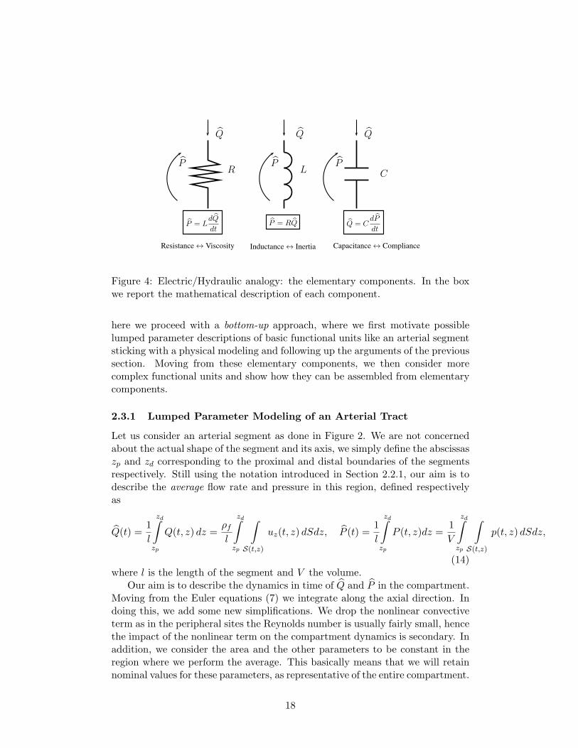
Resistance ↔ Viscosity Inductance ↔ Inertia Capacitance ↔ Compliance
Figure 4: Electric/Hydraulic analogy: the elementary components. In the boxwe report the mathematical description of each component.
here we proceed with a bottom-up approach, where we first motivate possiblelumped parameter descriptions of basic functional units like an arterial segmentsticking with a physical modeling and following up the arguments of the previoussection. Moving from these elementary components, we then consider morecomplex functional units and show how they can be assembled from elementarycomponents.
2.3.1 Lumped Parameter Modeling of an Arterial Tract
Let us consider an arterial segment as done in Figure 2. We are not concernedabout the actual shape of the segment and its axis, we simply define the abscissaszp and zd corresponding to the proximal and distal boundaries of the segmentsrespectively. Still using the notation introduced in Section 2.2.1, our aim is todescribe the average flow rate and pressure in this region, defined respectivelyas
Q(t) =1
l
zd∫
zp
Q(t, z) dz =ρfl
zd∫
zp
∫
S(t,z)
uz(t, z) dSdz, P (t) =1
l
zd∫
zp
P (t, z)dz =1
V
zd∫
zp
∫
S(t,z)
p(t, z) dSdz,
(14)where l is the length of the segment and V the volume.
Our aim is to describe the dynamics in time of Q and P in the compartment.Moving from the Euler equations (7) we integrate along the axial direction. Indoing this, we add some new simplifications. We drop the nonlinear convectiveterm as in the peripheral sites the Reynolds number is usually fairly small, hencethe impact of the nonlinear term on the compartment dynamics is secondary. Inaddition, we consider the area and the other parameters to be constant in theregion where we perform the average. This basically means that we will retainnominal values for these parameters, as representative of the entire compartment.
18
If we take the longitudinal average of the tract on the momentum equation,we loose any space dependence and obtain the ordinary differential equation
ρf l
A0
dQ
dt+ρfKRl
A20
Q+ Pd − Pp = 0, (15)
where Pd and Pp are the distal and proximal pressure, respectively. When takingthe longitudinal average of the mass conservation law, under the assumption thatthe time variations of pressure are linearly proportional to the time variation ofthe area, we obtain [146]
√A0l
β
dP
dt+ Qd − Qp = 0, (16)
where Qd and Qp are the distal and proximal flow rate, respectively.The two equations (15)-(16) represent a compartment model for an arterial
tract. Notice how three main effects are driving the motion of blood, (i) theblood inertia, (ii) the interaction with the wall, and (iii) the viscous resistance.While these effects are distributed along the 1D domain in the Euler equations(7), they are lumped in specific terms of the equations (15)-(16). In fact, the
term LdQ
dt, with L =
ρf l
A0, corresponds to the blood acceleration, so it is an
inertial term. The algebraic term RQ, with R =ρfKRl
A20
, stems from the blood
viscosity, while CdP
dt, with C =
√A0l
β, is due to the time variation of the section
as a consequence of fluid-structure interaction.Systems formally similar to (15)-(16) occur in different fields of applied math-
ematics. For instance they are obtained when studying the equations of a hy-draulic network [97] (with a coupling of 1D-0D models) and of a co-axial cable(see e.g. [174, 155]). In this respect, it is possible (and popular) to establish ananalogy between terms in the electrical as well as in the fluid-dynamics contexts,where the role of the flow rate for fluid-dynamics is played by the current, andthe pressure is corresponded by the voltage. This allows to adopt the symbol-ism of electrical circuits also in modeling the circulation. In particular, the threecontributions mentioned above are mathematically described by simple algebraicand differential equations, stated in the Table 2.3.1. The corresponding symbolsin Circuits Theory are depicted in Fig. 4.
The parameters involved in these equations depend on the specific featuresof the arterial tract. For instance, if we assume a circular cylinder with radiusR0 and a Poiseuille like flow, we obtain the following parameters [146],
R =8µl
πr40, L =
ρf l
πR20
, C =3πR3
0l
2EHs.
19
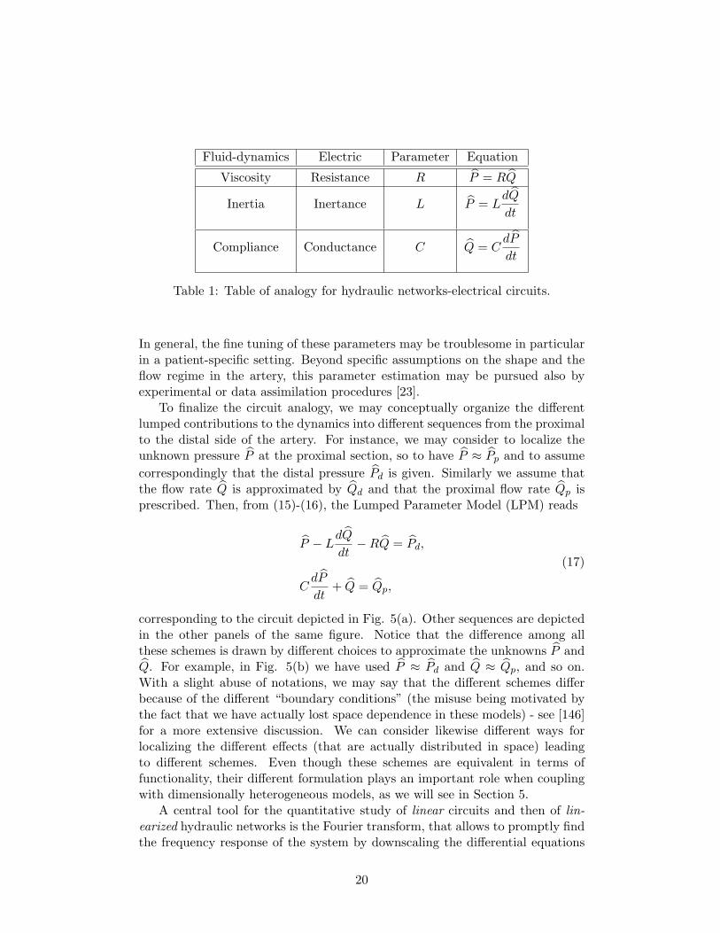
Fluid-dynamics Electric Parameter Equation
Viscosity Resistance R P = RQ
Inertia Inertance L P = LdQ
dt
Compliance Conductance C Q = CdP
dt
Table 1: Table of analogy for hydraulic networks-electrical circuits.
In general, the fine tuning of these parameters may be troublesome in particularin a patient-specific setting. Beyond specific assumptions on the shape and theflow regime in the artery, this parameter estimation may be pursued also byexperimental or data assimilation procedures [23].
To finalize the circuit analogy, we may conceptually organize the differentlumped contributions to the dynamics into different sequences from the proximalto the distal side of the artery. For instance, we may consider to localize theunknown pressure P at the proximal section, so to have P ≈ Pp and to assume
correspondingly that the distal pressure Pd is given. Similarly we assume thatthe flow rate Q is approximated by Qd and that the proximal flow rate Qp isprescribed. Then, from (15)-(16), the Lumped Parameter Model (LPM) reads
P − LdQ
dt−RQ = Pd,
CdP
dt+ Q = Qp,
(17)
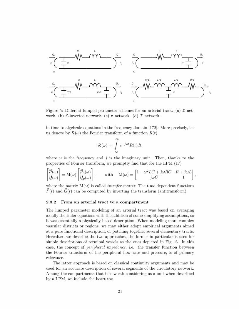
corresponding to the circuit depicted in Fig. 5(a). Other sequences are depictedin the other panels of the same figure. Notice that the difference among allthese schemes is drawn by different choices to approximate the unknowns P andQ. For example, in Fig. 5(b) we have used P ≈ Pd and Q ≈ Qp, and so on.With a slight abuse of notations, we may say that the different schemes differbecause of the different “boundary conditions” (the misuse being motivated bythe fact that we have actually lost space dependence in these models) - see [146]for a more extensive discussion. We can consider likewise different ways forlocalizing the different effects (that are actually distributed in space) leadingto different schemes. Even though these schemes are equivalent in terms offunctionality, their different formulation plays an important role when couplingwith dimensionally heterogeneous models, as we will see in Section 5.
A central tool for the quantitative study of linear circuits and then of lin-earized hydraulic networks is the Fourier transform, that allows to promptly findthe frequency response of the system by downscaling the differential equations
20
Qp
a)
Q
b)
QdQ
P
P1
Pd
P2
Pp
Pp Pd
P
L
L L/2
L
C
c) d)
Q2Q1Qp Qd
C/2
R
C/2
C
C
R
R
L/2 R/2R/2
Figure 5: Different lumped parameter schemes for an arterial tract. (a) L net-work. (b) L-inverted network. (c) π network. (d) T network.
in time to algebraic equations in the frequency domain [172]. More precisely, letus denote by R(ω) the Fourier transform of a function R(t),
R(ω) =
∞∫
−∞
e−jωtR(t)dt,
where ω is the frequency and j is the imaginary unit. Then, thanks to theproperties of Fourier transform, we promptly find that for the LPM (17)[P(ω)
Q(ω)
]= M(ω)
[Pd(ω)Qp(ω)
], with M(ω) =
[1− ω2LC + jωRC R+ jωL
jωC 1
],
where the matrix M(ω) is called transfer matrix. The time dependent functionsP (t) and Q(t) can be computed by inverting the transform (antitransform).
2.3.2 From an arterial tract to a compartment
The lumped parameter modeling of an arterial tract was based on averagingaxially the Euler equations with the addition of some simplifying assumptions, soit was essentially a physically based description. When modeling more complexvascular districts or regions, we may either adopt empirical arguments aimedat a pure functional description, or patching together several elementary tracts.Hereafter, we describe the two approaches, the former in particular is used forsimple descriptions of terminal vessels as the ones depicted in Fig. 6. In thiscase, the concept of peripheral impedance, i.e. the transfer function betweenthe Fourier transform of the peripheral flow rate and pressure, is of primaryrelevance.
The latter approach is based on classical continuity arguments and may beused for an accurate description of several segments of the circulatory network.Among the compartments that it is worth considering as a unit when describedby a LPM, we include the heart too.
21
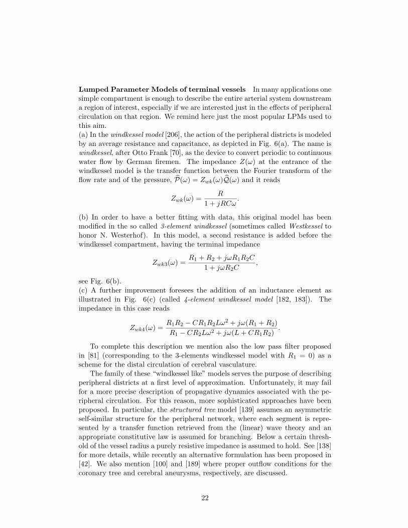
Lumped Parameter Models of terminal vessels In many applications onesimple compartment is enough to describe the entire arterial system downstreama region of interest, especially if we are interested just in the effects of peripheralcirculation on that region. We remind here just the most popular LPMs used tothis aim.(a) In the windkessel model [206], the action of the peripheral districts is modeledby an average resistance and capacitance, as depicted in Fig. 6(a). The name iswindkessel, after Otto Frank [70], as the device to convert periodic to continuouswater flow by German firemen. The impedance Z(ω) at the entrance of thewindkessel model is the transfer function between the Fourier transform of theflow rate and of the pressure, P(ω) = Zwk(ω)Q(ω) and it reads
Zwk(ω) =R
1 + jRCω.
(b) In order to have a better fitting with data, this original model has beenmodified in the so called 3-element windkessel (sometimes called Westkessel tohonor N. Westerhof). In this model, a second resistance is added before thewindkessel compartment, having the terminal impedance
Zwk3(ω) =R1 +R2 + jωR1R2C
1 + jωR2C,
see Fig. 6(b).(c) A further improvement foresees the addition of an inductance element asillustrated in Fig. 6(c) (called 4-element windkessel model [182, 183]). Theimpedance in this case reads
Zwk4(ω) =R1R2 − CR1R2Lω
2 + jω(R1 +R2)
R1 − CR2Lω2 + jω(L+ CR1R2).
To complete this description we mention also the low pass filter proposedin [81] (corresponding to the 3-elements windkessel model with R1 = 0) as ascheme for the distal circulation of cerebral vasculature.
The family of these “windkessel like” models serves the purpose of describingperipheral districts at a first level of approximation. Unfortunately, it may failfor a more precise description of propagative dynamics associated with the pe-ripheral circulation. For this reason, more sophisticated approaches have beenproposed. In particular, the structured tree model [139] assumes an asymmetricself-similar structure for the peripheral network, where each segment is repre-sented by a transfer function retrieved from the (linear) wave theory and anappropriate constitutive law is assumed for branching. Below a certain thresh-old of the vessel radius a purely resistive impedance is assumed to hold. See [138]for more details, while recently an alternative formulation has been proposed in[42]. We also mention [100] and [189] where proper outflow conditions for thecoronary tree and cerebral aneurysms, respectively, are discussed.
22
CC R
R1
R2
R1
R2CCL
Qw
pwp3w
Q3w
Q4w
p4w
QL
Figure 6: Lumped parameter models of terminal vessels. (a) windkessel; (b)3-element windkessel; (c) 4-element windkessel.
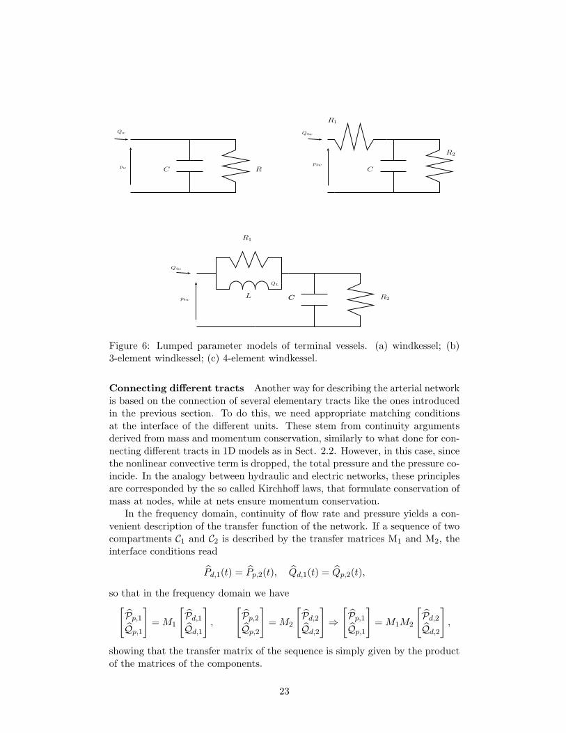
Connecting different tracts Another way for describing the arterial networkis based on the connection of several elementary tracts like the ones introducedin the previous section. To do this, we need appropriate matching conditionsat the interface of the different units. These stem from continuity argumentsderived from mass and momentum conservation, similarly to what done for con-necting different tracts in 1D models as in Sect. 2.2. However, in this case, sincethe nonlinear convective term is dropped, the total pressure and the pressure co-incide. In the analogy between hydraulic and electric networks, these principlesare corresponded by the so called Kirchhoff laws, that formulate conservation ofmass at nodes, while at nets ensure momentum conservation.
In the frequency domain, continuity of flow rate and pressure yields a con-venient description of the transfer function of the network. If a sequence of twocompartments C1 and C2 is described by the transfer matrices M1 and M2, theinterface conditions read
Pd,1(t) = Pp,2(t), Qd,1(t) = Qp,2(t),
so that in the frequency domain we have[Pp,1Qp,1
]=M1
[Pd,1Qd,1
],
[Pp,2Qp,2
]=M2
[Pd,2Qd,2
]⇒[Pp,1Qp,1
]=M1M2
[Pd,2Qd,2
],
showing that the transfer matrix of the sequence is simply given by the productof the matrices of the components.
23
♥t♦r ♥t♦r ♠ ❲ss
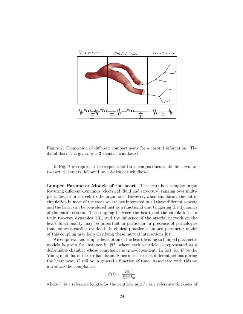
Figure 7: Connection of different compartments for a carotid bifurcation. Thedistal district is given by a 3-element windkessel.
In Fig. 7 we represent the sequence of three compartments, the first two aretwo arterial tracts, followed by a 3-element windkessel.
Lumped Parameter Models of the heart The heart is a complex organfeaturing different dynamics (electrical, fluid and structure) ranging over multi-ple scales, from the cell to the organ one. However, when simulating the entirecirculation in most of the cases we are not interested in all these different aspectsand the heart can be considered just as a functional unit triggering the dynamicsof the entire system. The coupling between the heart and the circulation is atruly two-way dynamics [131] and the influence of the arterial network on theheart functionality may be important in particular in presence of pathologiesthat induce a cardiac overload. In clinical practice a lumped parameter modelof this coupling may help clarifying these mutual interactions [61].
An empirical and simple description of the heart leading to lumped parametermodels is given for instance in [92] where each ventricle is represented as adeformable chamber whose compliance is time-dependent. In fact, let E be theYoung modulus of the cardiac tissue. Since muscles exert different actions duringthe heart beat, E will be in general a function of time. Associated with this weintroduce the compliance
C(t) =2πl30E(t)h0
,
where l0 is a reference length for the ventricle and h0 is a reference thickness of
24
♦ ♠
P P
♦♦
❱ ❱
s
ss t
tt r ♣
♥
♥
PP P
②
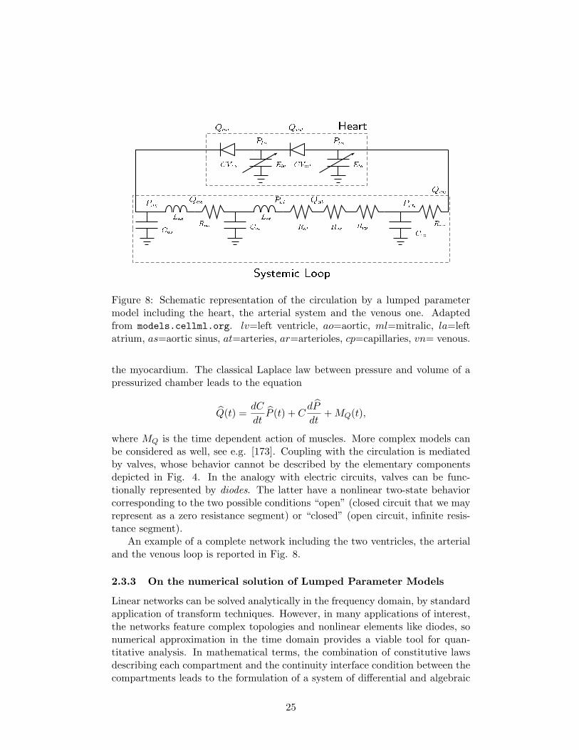
Figure 8: Schematic representation of the circulation by a lumped parametermodel including the heart, the arterial system and the venous one. Adaptedfrom models.cellml.org. lv=left ventricle, ao=aortic, ml=mitralic, la=leftatrium, as=aortic sinus, at=arteries, ar=arterioles, cp=capillaries, vn= venous.
the myocardium. The classical Laplace law between pressure and volume of apressurized chamber leads to the equation
Q(t) =dC
dtP (t) + C
dP
dt+MQ(t),
where MQ is the time dependent action of muscles. More complex models canbe considered as well, see e.g. [173]. Coupling with the circulation is mediatedby valves, whose behavior cannot be described by the elementary componentsdepicted in Fig. 4. In the analogy with electric circuits, valves can be func-tionally represented by diodes. The latter have a nonlinear two-state behaviorcorresponding to the two possible conditions “open” (closed circuit that we mayrepresent as a zero resistance segment) or “closed” (open circuit, infinite resis-tance segment).
An example of a complete network including the two ventricles, the arterialand the venous loop is reported in Fig. 8.
2.3.3 On the numerical solution of Lumped Parameter Models
Linear networks can be solved analytically in the frequency domain, by standardapplication of transform techniques. However, in many applications of interest,the networks feature complex topologies and nonlinear elements like diodes, sonumerical approximation in the time domain provides a viable tool for quan-titative analysis. In mathematical terms, the combination of constitutive lawsdescribing each compartment and the continuity interface condition between thecompartments leads to the formulation of a system of differential and algebraic
25
equations (DAE systems) that takes the form
Ady
dt+ f(t,y, z) = g(t), (18a)
Gy +Mz = c(t), (18b)
t > 0. Here y is the set of n variables whose time dynamics describes the stateof the system (pressure and flow rates in the different locations of the networkassociated with capacitance and inductance effects respectively) and z is a vectorof m additional variables needed to close the description of the network by theapplication of the balance conditions (Kirchhoff laws, given by (18b)); A is an × n matrix, G is m × n and M is m × m. The term f(t,y, z) is in generalnonlinear for the presence of diodes. g and c represent forcing terms. We assumethat initial conditions y(0) = y0 are prescribed at t = 0. In the case of interestfor cardiovascular applications, the square matrix M is generally nonsingular.This qualifies system (18) as an index 1 DAE system and we may reduce it to aclassical Cauchy problem
Ady
dt+ f(t,y,M−1(c−Gy)) = g(t),
y(0) = y0,
for which several well established numerical methods exist [36]. Among theothers we mention Runge Kutta methods that are particularly prone to time-adaptive strategies that allow an automatic selection of the time discretizationstep to fulfill user-defined accuracy requirements. We do not enter into detailshere, the interested reader is referred to [108, 162].
2.3.4 Further developments
The actual functioning of the circulatory system includes effects that cannotbe simply described by fluid-dynamics and fluid-structure interaction equations.Living systems adapt to different conditions. For instance, running requiresan increment in oxygen delivery to lower limbs that may be obtained by anincrement of the blood pumping rate and a vasodilation in the districts interestedby the physical exercise. These regulatory dynamics involve the interactionbetween fluid, mechanics and chemical reactions occurring in several parts ofthe network according to different mechanisms. For instance, a constant oxygendelivery to the brain tissues is guaranteed by complex dynamics that go underthe name of autoregulation.
A comprehensive description of these aspects is out of the scope of the presentwork. We remind however that lumped parameter models are particularly fittedto provide quantitative models since they are able of covering large portions ofthe network and of providing simple but reliable empirical models of complexdynamics occurring at different time scales. The interested reader is referred to[140, 146] and the references therein mentioned.
26
3 Boundary conditions: what we have, what is miss-
ing
When solving blood flow problems with any of the stand-alone models introducedin the previous section, we are faced with the issue of the data to be prescribedas boundary conditions for the 3D and 1D models or as forcing terms (thatsurrogate boundary conditions) for 0D models.
In clinical settings, data are retrieved from in vivo measures. This can bedone in many different ways and an extensive analysis of possible sources ofdata is certainly out of scope of the present work. In general, measures mayrefer to pointwise velocities on a (strict) subset of inflow/outflow boundariesof a vascular district (e.g. with PC-MRI) or indirectly to average quantitieslike the flow rate over a section; for the pressure, data (in particular obtainedby noninvasive measures) are almost invariably an average information over asection of interest. Quite often there are practical difficulties in retrieving dataat the distal (outlet) boundaries and no patient-specific information is available.These practical problems clearly add specific issues to the boundary treatmentof mathematical and numerical models.
Specifically, if we are using a 3D model in deformable domains that corre-spond to tracts of arteries that are artificially truncated, the correct prescriptionof boundary conditions needs to address several concerns. On the one hand, weneed to prescribe conditions consistent with the propagation dynamics describedby the FSI that in particular avoid spurious reflections at the outlets. On theother hand, partial (or absent) measures need to be properly completed to makethe 3D model well posed. The additional - somehow arbitrary - conditions needto be consistent with the physical problem. This is discussed in Sect. 3.1.
When dealing with 1D models, the lack of boundary data is in general lesstroublesome (as a matter of fact, one average-in-space quantity per boundarypoint makes the continuous problem well-posed). However, the hyperbolic na-ture of the 1D model still raises issues of prescribing conditions at the outletsin a way consistent with the propagation dynamics. In addition, numerical dis-cretization usually requires extra conditions that are absent in the continuousproblem, yet need to be retrieved in a way consistent with the orignal model.This calls for special care for boundary treatment as we will see in Sect. 3.2.
Finally, we have already pointed out that in spite of the lack of space de-pendence in 0D models, prescription of input physically corresponds to localizeddata and the type of those data needs to be compatible with the nature of thelumped parameter model. This is discussed in Sect. 3.3.
3.1 3D defective boundary problems
Mathematical theory of the incompressible Navier-Stokes equations states thatwe need to prescribe three scalar conditions at each point of the boundary.This is almost invariably impossible in clinical settings. As pointed out, phase-
27
contrast MRI provides for instance velocity data only in selected points of avascular domain that typically do not cover the entire entrance section Γ of avascular district [127]. Alternatively, the flow rate Q(t) can be obtained at Γ byproper elaboration of data retrieved e.g. by the Echo-Doppler technique basedon ultrasound [175] or by thermal images [114] - see also [208, 99]. Moreover,as we will see in Sect. 4 and 5, the prescription of defective data for the 3Dmodel is a crucial issue in view of the geometric multiscale approach we are herereviewing. For all these reason, we consider the following flow rate condition
ρf
∫
Γu · n dγ = Q. (19)
Similarly, at both the inlet and outlet sections available pressure data P (t) areconsidered representative of an average estimate, i.e. we have
1
|Γ|
∫
Γp dγ = P. (20)
Conditions (19) and (20) are called defective in the sense that they prescribejust one scalar function over the entire section Γ, marking a clear gap betweentheory and practice that needs to be filled up to get quantitative solutions to theproblem. Hereafter we illustrate some of the most common strategies to pursuethis goal.
3.1.1 Flow rate condition
Empirical approach. The most immediate way to prescribe condition (19)consists in choosing a velocity profile g such that for each t
ρf
∫
Γg(t) · n dγ = Q(t). (21)
In this way, flow rate data are converted into standard Dirichlet conditions. Thisis a popular strategy in computational hemodynamics. Classical choices for thevelocity profile are the parabolic one, which works very well for example for flowsimulations in the carotids [37], the flat one, which is quite often used for theascending aorta [126], and the one based on the Womersley solution. Noticethat both the parabolic and Womersley profiles require a circular section to beprescribed on. Non-circular sections require an appropriate morphing [84].
Unfortunately, in spite of its straightforward implementation, the a priori andarbitrary assumption on the velocity profile has a major impact on the solution,in particular in the neighborhood of the section. To reduce the sensitivity of theresults to the arbitrary choice of the profile, the computational domain can beartificially elongated by the so called flow extensions, thus involving additionalcomputational burden.
28
Augmented formulation based on Lagrange multipliers: rigid walls.The augmented formulation was proposed in [59] for the case of rigid walls andfor a steady/linear Stokes fluid model. Following this approach the flow rateboundary condition (19) is regarded as a constraint for the solution of the fluidproblem. As such it is enforced by a Lagrange multiplier approach in a waysimilar to the incompressibility. Being a scalar constraint, we need a scalarmultiplier λ, resulting in the following weak formulation: Find u ∈ V, p ∈ Qand λ ∈ R such that for all v ∈ V, q ∈ Q and ψ ∈ R, it holds
µ(∇u+ (∇u)T ,∇v
)− (p,∇ · v) + λ
∫
Γv · n dγ = F (v),
(q,∇ · u) = 0,
ψρf
∫
Γu · n dγ = ψQ,
(22)
where V = v ∈ (H1(Ωf ))3 : v|ΣD
= 0, ΣD being the portion of the boundarywhere Dirichlet conditions are prescribed, Q = L2(Ω), F accounts for possiblenon-homogeneous Dirichlet and/or Neumann conditions on ∂Ωf \ Γ, and (·, ·)denotes the L2 inner product.
It is possible to prove that beyond the flow rate condition (19)
1. the augmented formulation prescribes a constant traction on Γ alignedwith its normal direction;
2. the constant coincides with the Lagrange multiplier λ,
that means−pn+ µ
(∇u+ (∇u)T
)n = λn on Γ.
From the quantitative view point, the overall result is that a constant-in-space traction is prescribed (the constant being unknown) resulting in a lessstringent condition than the Dirichlet one of the empirical approach. Thismethod is particularly suited when the artificial cross section is orthogonal tothe longitudinal axis, so that vector n is truly aligned along the axial direc-tion. Generalization of this strategy to the unsteady/non-linear case can befound in [195], the unknown Lagrange multiplier variable being a function oftime (λ = λ(t)). Inf-sup condition for the twofold saddle point problem (22) isproved [195].
For the numerical solution of this formulation, one could rely either on amonolithic strategy where the full augmented matrix is built and solved, or onsplitting techniques. In particular, in [59, 195] it is proposed to write the Schurcomplement scalar equation with respect to the Lagrange multiplier, leading toan algorithm where two standard fluid problems with Neumann conditions onΓ need to be solved at each time step (exact splitting technique). The latterapproach preserves modularity, that is it could be implemented using avail-able standard legacy fluid solvers in a black box fashion. This is an interesting
29
property in view of the application to cases of real interest, as done e.g. in[203, 200, 154].
To reduce the computational time needed by the exact splitting approach,in [196] a different splitting procedure is proposed, which introduces an errornear the boundary that is however always remarkably smaller than the oneproduced by the empirical approach. This strategy (called inexact splitting
technique) requires the solution of just one standard fluid problem at each timestep, thus halving the computational time with respect to that of the exactsplitting technique.
To extend the augmented approach to the case of n flow rate conditions oneLagrange multiplier has to be introduced for each condition. In this case, theexact splitting procedure requires the solution of n + 1 fluid problems at eachtime step (see [59]), whereas the inexact procedure still needs to solve just onefluid problem.
Another approach, holding for the case of single as well as multiple flow rateconditions, is to perform an appropriate factorization of the augmented algebraicsystem that allows to reduce the computational costs with no extra errors, asrecently addressed in [130].
The augmented formulation has been extended to the quasi-Newtonian casein [52].
Augmented formulation: compliant walls. The extension of the aug-mented formulation to the case of compliant walls is addressed in [67]. There arebasically two strategies we may consider. In the former (“split-then-augment”)we first split the fluid-structure interaction problem in a segregated way, so toapply the augmentation procedure to the fluid subproblem at each iteration ofthe partitioned algorithm. In this case, one of the approaches described for therigid case can be applied straightforwardly. This method is successfully consid-ered in real settings in [159].
In the latter strategy (“augment-then-split”) we directly perform the aug-mentation on the FSI problem. At the numerical level, we still have the optionof pursuing either a monolithic or a partitioned approach. In the former case,suitable preconditioners are mandatory [44]. In the latter one, the problem canbe formally reduced to the Schur complement equation for the sole λ. This ac-tually implies at each time step the solution of two standard FSI problems withNeumann conditions on Γ, thus preserving modularity with respect to availableFSI legacy solvers [67].
3.1.2 Mean pressure boundary conditions
To prescribe the mean pressure condition (20) we can follow an approach similarto the empirical one, where a velocity profile is arbitrarily selected to fulfill thegiven flow rate. In this case, we can postulate that the pressure on Γ is constant
30
and that the normal viscous stress can be discarded, so that
pn− µ(∇u+ (∇u)T
)n = Pn on Γ. (23)
The previous assumption is generally acceptable because the pressure changesin arteries mainly occur along the axial direction.
This approach results in the prescription of a standard Neumann condition,being the average pressure considered as the boundary traction. In the processof numerical discretization, for P = 0 it requires no further action than justassembling the matrix for homogeneous Neumann conditions. Therefore this hasbeen called “do-nothing” approach [87]. This name is suggestive, however it hasto be kept in mind that an “action” is actually performed (even if implicitly) [194,193]. For instance, for the Stokes problem, the do-nothing approach correspondsto the following weak formulation (for the sake of simplicity we still refer to thesteady case): Find u ∈ V and p ∈ Q such that for all v ∈ V and q ∈ Q, it holds
µ(∇u+ (∇u)T ,∇v
)− (p,∇ · v) = −P
∫
Γv · n dγ + F (v),
(q,∇ · u) = 0,(24)
where we have used the same notation introduced for the augmented formula-tion (22). Even if (23) is an approximation, for a section Γ orthogonal to the
longitudinal direction the contribution
∫
Γµ(∇u+ (∇u)T
)n dγ is in general
expected to be very small if compared to∫Γ p dγ.
Besides the grad-grad formulation (24), other weak formulations may be con-sidered as well for the do-nothing approach, for example the curl-curl formulation
having the pressure as natural condition. In this case, the do-nothing approachcorresponds to the boundary condition
p = P on Γ,
the only assumption being that the pressure is constant on Γ, without any furtherrequest on the smallness of the viscous boundary term (see [41, 194, 195]).
Remark 1. In principle, also mean pressure conditions (20) can be enforcedusing a Lagrange multiplier approach, as done for the flow rate problem. In asomehow dual situation to the case of flow rate conditions, the Lagrange mul-tiplier in this case represents the normal velocity to the section Γ and the aug-mented approach is implicitly forcing it to be constant in space. While a constantpressure over Γ is an acceptable approximation, the same is not true for a normalconstant velocity. For this reason, the augmented Lagrange multiplier approachfor mean pressure conditions does not represent a reliable option.
Remark 2. A do-nothing formulation for the flow rate conditions is possibletoo, see [87, 194]. As a matter of fact, this was the first attempt to provide
31
a mathematically sound formulation to the flow rate problem. This approachrelies on the introduction of a set of functions that represents the lifting of theflow rate data inside the domain, in a way similar to what is done for standardDirichlet conditions. See also [41] for a curl-curl formulation. However, the lift-ing functions, called flux-carriers, are not easy to construct in general. Becauseof that, the do-nothing approach for flow rate conditions is not very popular.Nevertheless, it is worth noting that this formulation implies that the tractionon Γ is constant and aligned with its normal - see [194] - as for the solutionfound with the Lagrange multiplier approach. We argue therefore that the do-nothing approach for flow rate conditions computes the same solution found bythe augmented formulation (22).
Remark 3. A popular weak formulation of the incompressible Navier-Stokesequations discards the divergence free term (∇u)T in the definition of the fluidCauchy stress tensor (2), so for a constant viscosity we have ∇ · (µ (∇u)T ) = 0.This allows to have a block-diagonal pattern in the corresponding Finite Elementstiffness matrix arising after space discretization. It is pointed out in [87] thatwith this simplified formulation, the associated do-nothing condition at Γ, pn−µ∇un = Pn, is more appropriate for artificial boundaries than (23), since itcomputes correctly the Poiseuille solution - as opposed to the case with the term(∇u)T . In [194, 193] it is however pointed out how mixed Dirichlet/Neumannconditions at the artificial boundary (prescribing Neumann conditions only in thenormal direction and homogeneous Dirichlet in the tangential ones) can correctlycapture the Poiseuille solution even with the complete formulation of the fluidstress tensor.
3.1.3 A control-based approach
A different strategy for the fulfillment of condition (19) is based on the mini-mization of the mismatch functional
J(v) =1
2
(∫
Γv · n dγ −Q
)2
, (25)
constrained by the fact that v satisfies the incompressible Navier Stokes equa-tions [66].
This strategy is somehow the dual of the augmented strategy, where the de-fective boundary data were considered as a constraint to the energy minimizationof the fluid. Instead, in the current approach the aim is to minimize (25) with theconstraint given by the fluid equations. The constrained minimization problemleads to the Karush-Kuhn-Tucker (KKT) conditions, whose numerical solutioncan be obtained by iterative algorithms. In particular in [66] the normal tractionon Γ is used as control variable for the minimization of the mismatch functional.
In [67], this approach is considered for the compliant case. In particular,a fast algorithm based on a convenient combination of the iterations of the
32
partitioned FSI solver and of the constrained minimization has been introduced.In [109, 73, 74], the extensions to the non-Newtonian, quasi-Newtonian, andvisco-elastic cases are addressed.
The same approach can also be used to fulfill the mean pressure conditions(20) over one or several boundary sections. This allows to prescribe a meanpressure condition on a section oblique with respect to the longitudinal axis too.In this case the control variable is the complete traction vector, that is also thedirection of the traction is a priori unknown [66].
Two-dimensional numerical results highlight the accuracy of the control-based approach for the prescription of both defective conditions (19) and (20)at a computational cost which is comparable with the one featured by the exactsplitting strategy introduced to solve the augmented problem.
Remark 4. The above constrained minimization approach resembles variationalmethods of Data Assimilation - see e.g. [47, 48, 20, 197]. In this variationalcontext, a further possibility consists of including in (25) some sparse measuresavailable not only on the boundary but also inside the region of interest. The aimcould be to either driving the solution to match (in some sense) these data [48],possibly including stochastic information on the measurement error to quantifythe uncertainty affecting the final assimilation [49], or obtaining a better estimateof one or more parameters of physical interest, e.g. the wall compliance [148,21, 207].
3.1.4 Further developments and comments
A defective Nitsche-like approach. The original idea of Nitsche of prescrib-ing Dirichlet conditions with a penalization approach [132] has been recentlyextended to the case of flow rate boundary conditions in [209]. This strategydoes not augment the variables of the original problem, however it introducesa parameter for the penalization that needs to be properly tuned. In addition,it deals with non standard bilinear forms that require ad hoc implementation.Two dimensional numerical results shown in [209] highlight the accuracy of themethod, whereas three-dimensional results reported in [158] demonstrate thatthis is an effective approach for real applications. A similar approach has beenextended to fulfill the mean pressure condition (20) and the FSI case in [198].
Defective boundary conditions for the structure. In some circumstances,boundary information available on the (artificial) arterial cross section (indicatedby the circular annulus Γs in Figure 9) might be insufficient to provide theboundary conditions that are required to “close” the structure problem. Thisis e.g. the case where the only data available is the area of the cross-sectionallumen Γ, that is the real number (function of t) A(t). In this case we have
∫
Γ(t)r dr dϕ =
∫ 2π
0
∫ R0(ϕ)+ηr(t,ϕ)
0r dr dϕ = A(t), (26)
33
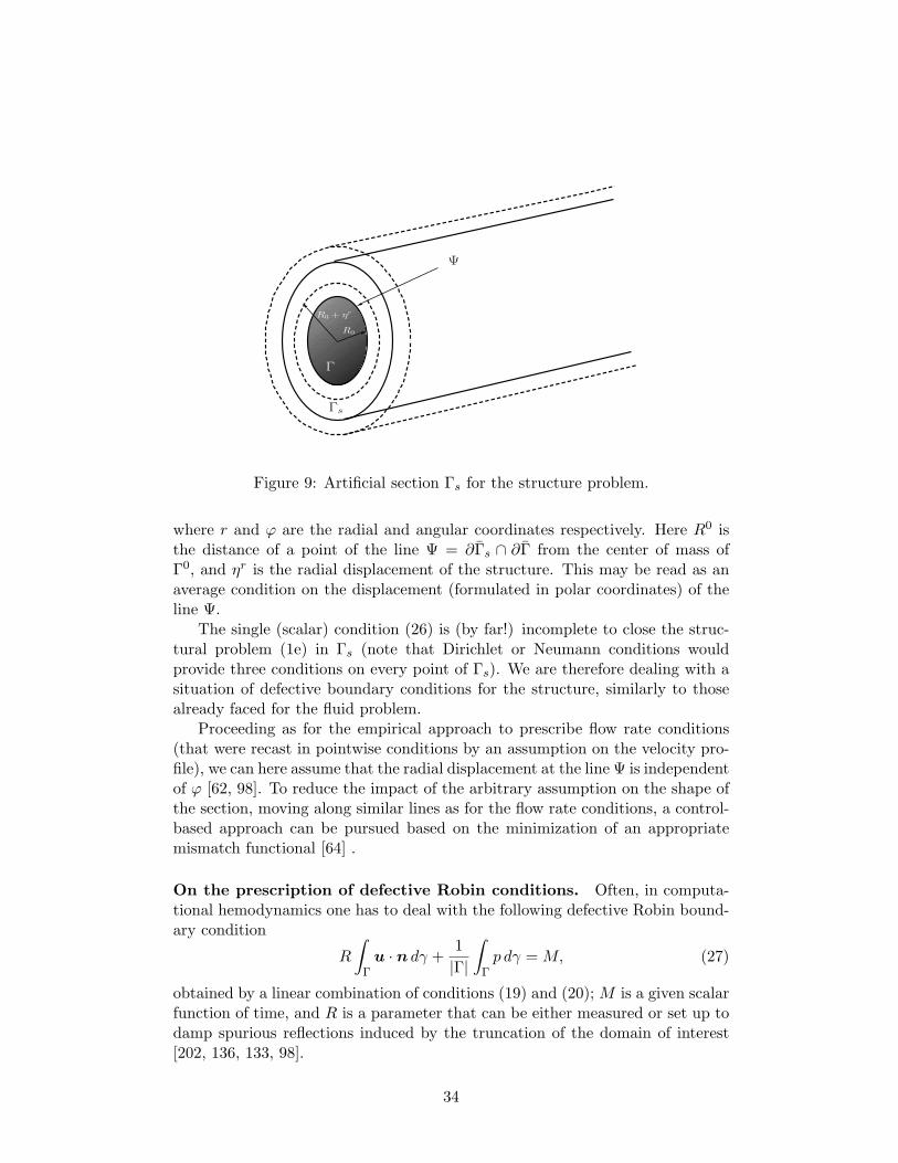
Ψ
Γ
R0
R0 + ηr
Γs
Figure 9: Artificial section Γs for the structure problem.
where r and ϕ are the radial and angular coordinates respectively. Here R0 isthe distance of a point of the line Ψ = ∂Γs ∩ ∂Γ from the center of mass ofΓ0, and ηr is the radial displacement of the structure. This may be read as anaverage condition on the displacement (formulated in polar coordinates) of theline Ψ.
The single (scalar) condition (26) is (by far!) incomplete to close the struc-tural problem (1e) in Γs (note that Dirichlet or Neumann conditions wouldprovide three conditions on every point of Γs). We are therefore dealing with asituation of defective boundary conditions for the structure, similarly to thosealready faced for the fluid problem.
Proceeding as for the empirical approach to prescribe flow rate conditions(that were recast in pointwise conditions by an assumption on the velocity pro-file), we can here assume that the radial displacement at the line Ψ is independentof ϕ [62, 98]. To reduce the impact of the arbitrary assumption on the shape ofthe section, moving along similar lines as for the flow rate conditions, a control-based approach can be pursued based on the minimization of an appropriatemismatch functional [64] .
On the prescription of defective Robin conditions. Often, in computa-tional hemodynamics one has to deal with the following defective Robin bound-ary condition
R
∫
Γu · n dγ +
1
|Γ|
∫
Γp dγ =M, (27)
obtained by a linear combination of conditions (19) and (20); M is a given scalarfunction of time, and R is a parameter that can be either measured or set up todamp spurious reflections induced by the truncation of the domain of interest[202, 136, 133, 98].
34
The prescription of such a condition for R ∈ (0,+∞) is discussed in [202],where a monolithic approach has been proposed, in [68] for the case of theaugmented and control-based formulations, and in [198] for the Nitsche strategy.
Remark 5. Using Neumann conditions at the downstream artificial sectionsmight induce numerical instabilities. These are usually called backflow instabil-ities because they are typically triggered by the backflow in diastole at the outletsections of a vascular district, see [16, 124]. In this case, using a condition like(27) will “cure” the problem by setting the (nonlinear) parameter R to be activeonly in the presence of a normal velocity component incoming the domain.
Defective conditions alternative to the mean pressure. Another possi-ble defective condition prescribes the average traction (in place of the averagepressure as done in (20)):
1
|Γ|
∫
ΓT f (u, p)n · n dγ = T, (28)
for a given function of time T (t). Its actual implementation follows closely thatof condition (20). In particular, if a do-nothing approach is considered for (28),one obtains again formulation (24), which still actually prescribes condition (23),with the right hand side P replaced by T . However, in this case condition (23)is consistent with the defective condition (28) (unlike (20), see Sect. 3.1.2).
The optimal control approach can be applied for the prescription of (28)provided that a suitable functional is considered. In [67], numerical resultshighlight the differences between the solutions obtained with this strategy toprescribe condition (20) and (28). We observe that also the Nitsche-like methodcould be extended to prescribe condition (28), as shown in [198] .
In a similar way, given two functions of time Ptot(t) and Ttot(t), we canconsider defective conditions involving the total pressure
1
|Γ|
∫
Γptotdγ = Ptot,
or the mean total normal traction
1
|Γ|
∫
ΓT f (u, ptot)n · n dγ = Ttot,
whereptot = p+
ρf2|u|2 (29)
denotes the total pressure. Notice that using the identity
(u · ∇)u =1
2∇|u|2 + curlu× u, (30)
the natural boundary conditions associated with the Navier-Stokes problem in-volve the total pressure or the total traction. The do-nothing procedure can beperformed in these cases as done for the average pressure and traction (see, e.g.,[193, 194, 62]).
35
Applications of clinical interest. We conclude this section by mentioningsome practical applications of the strategies described above for the treatmentof defective boundary conditions, in particular the one based on the augmentedapproach.
This strategy has been successfully applied to investigate the jet impingingthe ascending aortic wall downstream a bicuspid aortic valve [203, 200], or in anabdominal aortic aneurysm to assess the viscous forces [154].
Another application is proposed in [156] to improve approximation of flowrate measurements obtained by ultrasound devices. Doppler velocimetry is cur-rently used to provide an estimate of the flow rate in a vascular district startingfrom the measurement of the maximum velocity. This estimate is based on theassumption of parabolic profile (Doucette formula). Despite its popularity andsimplicity, this formula relies on an unrealistic hypothesis, that of parabolic pro-file, which makes sense only for steady flows in rectilinear circular pipes. Thebasic idea in [156] is to extend the Doucette formula including the dependenceof the flow rate also on the pulsatility, by means of the Womersley number. Thefitting of the new formula is performed by running several numerical simulationsin different scenarios by applying the flow rate with the augmented approach.This choice is motivated by the necessity of finding a relation between flow rateand maximum velocity not biased by an a priori choice of the velocity profile.Results prove the reliability of this method, which has then been successivelyvalidated in clinical settings [199, 157].
3.2 The role of the Riemann variables for 1D models
When solving propagative equations like the 1D Euler system (7), a major prob-lem is the correct treatment of the boundary conditions. For instance, whenthe end points do not correspond to physical boundaries, non-reflecting condi-tions should be prescribed to the original continuous problem. With this wemean conditions that correctly describe the motion of the different propagativecomponents, without introducing any spurious effect like unphysical reflections.Moreover, after space discretization, the number of equations at the boundarypoints is not enough to close the system at the algebraic level. This demands formore numerical boundary conditions than those required by the original problemitself.
In this regard, a key concept is that of Riemann variables. We illustratethe role of Riemann variables on the single arterial tract represented by the 1D
system (7). Let us introduce the following notation: L =
[lT1lT2
], R = [r1 r2],
where l1, l2 and r1, r2 are the left and right eigenvectors of H. We can writetherefore H = RΛL, with Λ = diag(λ1, λ2). In addition, we define the Riemannvariables W1 and W2 as
∂W1
∂U= l1,
∂W2
∂U= l2. (31)
36
These are also called characteristic variables. Notice that, depending on thevessel law and on the assumptions on the parameters of the system, an explicitexpression of the characteristic variables as a function of the physical variables
Wi = ζi(A,Q), i = 1, 2, (32)
can be derived. For example, in the case α = 1 (with α the Coriolis coefficient,see Section 2.2.1) and for the algebraic law (11) we have [60]
W1,2 = ζ1,2(A,Q) =Q
A± 4
√β
2ρfA0A1/4,
where β is given by (11).After multiplication of (7) by L, we have the characteristic system
∂W
∂t+ Λ
∂W
∂z+G(W ) = 0 z ∈ (0, L), t > 0, (33)
with G = LB. Componentwise, these equations read
∂Wi
∂t+ λi
∂Wi
∂z+Gi(W1,W2) = 0, i = 1, 2.
After introducing the characteristic lines zi(t) for i = 1, 2, solution of the prob-lems
dzidt
= λi, i = 1, 2,
our problem readsdWi
dt
∣∣∣∣z=zi(t)
+Gi(W1,W2) = 0.
When G = 0 we have two independent problems, the Wi’s are constant alongtheir respective characteristic line and they are called Riemann invariants.
As we noticed in (10), the diagonal entries of Λ are λ1 > 0 and λ2 < 0. Thismeans that the Riemann variable W1 propagates forward along z, while W2 ismoving backward. Otherwise said, z = 0 (z = L) is an inflow end point for W1
(W2), so we need one boundary condition at each end point.A first possibility is given by prescribing conditions on the primary vari-
ables to system (7), i.e. the flow rate Q = Qm(t) or the area A = Am(t) (orequivalently the pressure).
Alternatively, one could consider the linearized system (33) and prescribeone of the characteristic variables Wi so as to obtain a non-reflecting condition.In particular, following [85, 188] by the theory of characteristics we have
∂W1
∂t+R1(W1,W2) = 0 at z = 0,
∂W2
∂t+R2(W1,W2) = 0 at z = L,
(34)
37
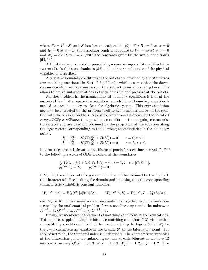
where Ri = lTi · S, and S has been introduced in (9). For R1 = 0 at z = 0and R2 = 0 at z = L, the absorbing conditions reduce to W1 = const at z = 0and W2 = const at z = L (with the constants given by the initial conditions)[60, 146].
A third strategy consists in prescribing non-reflecting conditions directly tosystem (7). In this case, thanks to (32), a non-linear combination of the physicalvariables is prescribed.
Alternative boundary conditions at the outlets are provided by the structuredtree modeling mentioned in Sect. 2.3 [139, 42], which assumes that the down-stream vascular tree has a simple structure subject to suitable scaling laws. Thisallows to derive suitable relations between flow rate and pressure at the outlets.
Another problem in the management of boundary conditions is that at thenumerical level, after space discretization, an additional boundary equation isneeded at each boundary to close the algebraic system. This extra-conditionneeds to be extracted by the problem itself to avoid inconsistencies of the solu-tion with the physical problem. A possible workaround is offered by the so-calledcompatibility conditions, that provide a condition on the outgoing characteris-tic variable and are basically obtained by the projection of the equation alongthe eigenvectors corresponding to the outgoing characteristics in the boundarypoints,
lT2 ·(∂U∂t +H(U)∂U∂z +B(U)
)= 0 z = 0, t > 0,
lT1 ·(∂U∂t +H(U)∂U∂z +B(U)
)= 0 z = L, t > 0.
In terms of characteristic variables, this corresponds for each time interval [tn, tn+1]to the following system of ODE localized at the boundaries
ddtWi(t, yi(t)) +Gi(W1,W2) = 0, i = 1, 2 t ∈ [tn, tn+1],y1(t
n+1) = L, y2(tn+1) = 0.
If Gi = 0, the solution of this system of ODE could be obtained by tracing backthe characteristic lines exiting the domain and imposing that the correspondingcharacteristic variable is constant, yielding
W2
(tn+1, 0
)=W2 (t
n, |λn2 (0)|∆t) , W1
(tn+1, L
)=W1 (t
n, L− λn1 (L)∆t) ,
see Figure 10. These numerical-driven conditions together with the ones pre-scribed by the mathematical problem form a non-linear system in the unknownsAn+1|z=0, Q
n+1|z=0, An+1|z=L, Qn+1|z=L.
Finally, we mention the treatment of matching conditions at the bifurcations.This requires supplementing the interface matching conditions (13) with furthercompatibility conditions. To find them out, referring to Figure 3, let W i
j be
the j−th characteristic variable in the branch Bi at the bifurcation point. Forease of notation, the temporal index is understood. The characteristic variablesat the bifurcation point are unknowns, so that at each bifurcation we have 12unknowns, namely Qi, i = 1, 2, 3, Ai, i = 1, 2, 3, W i
j , i = 1, 2, 3, j = 1, 2. The
38
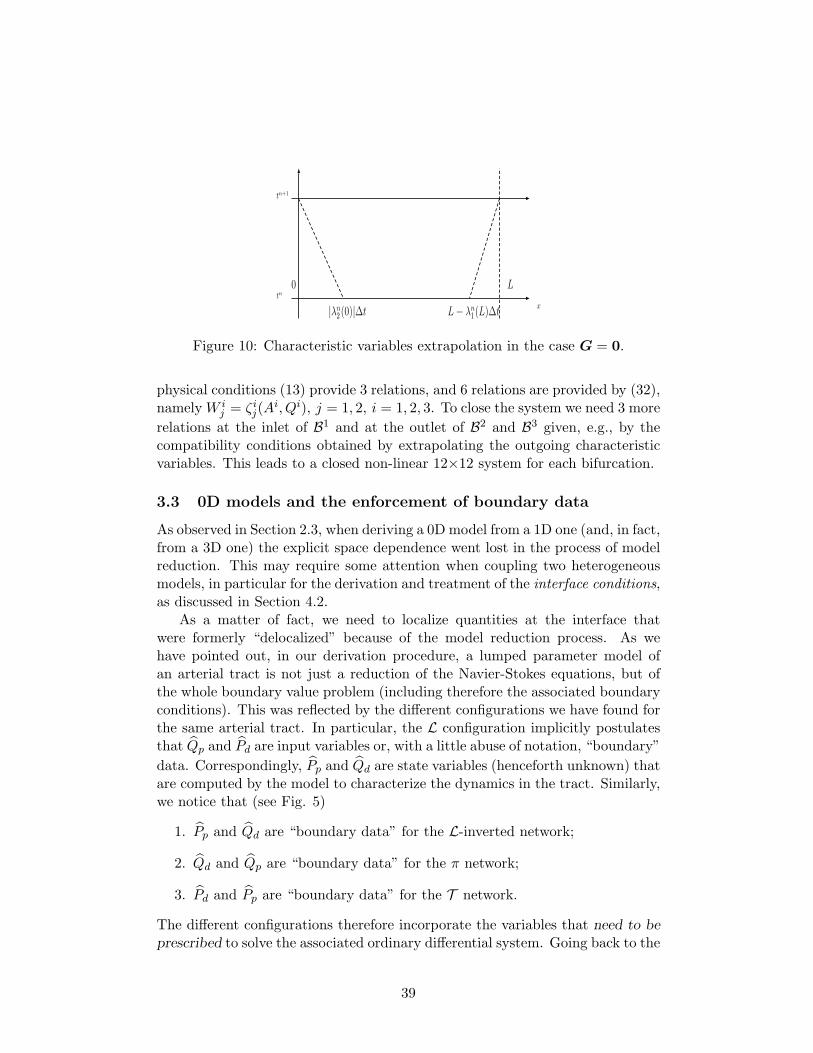
|λn2(0)|∆t L− λn
1(L)∆t
xtn
tn+1
0 L
Figure 10: Characteristic variables extrapolation in the case G = 0.
physical conditions (13) provide 3 relations, and 6 relations are provided by (32),namelyW i
j = ζij(Ai, Qi), j = 1, 2, i = 1, 2, 3. To close the system we need 3 more
relations at the inlet of B1 and at the outlet of B2 and B3 given, e.g., by thecompatibility conditions obtained by extrapolating the outgoing characteristicvariables. This leads to a closed non-linear 12×12 system for each bifurcation.
3.3 0D models and the enforcement of boundary data
As observed in Section 2.3, when deriving a 0D model from a 1D one (and, in fact,from a 3D one) the explicit space dependence went lost in the process of modelreduction. This may require some attention when coupling two heterogeneousmodels, in particular for the derivation and treatment of the interface conditions,as discussed in Section 4.2.
As a matter of fact, we need to localize quantities at the interface thatwere formerly “delocalized” because of the model reduction process. As wehave pointed out, in our derivation procedure, a lumped parameter model ofan arterial tract is not just a reduction of the Navier-Stokes equations, but ofthe whole boundary value problem (including therefore the associated boundaryconditions). This was reflected by the different configurations we have found forthe same arterial tract. In particular, the L configuration implicitly postulatesthat Qp and Pd are input variables or, with a little abuse of notation, “boundary”
data. Correspondingly, Pp and Qd are state variables (henceforth unknown) thatare computed by the model to characterize the dynamics in the tract. Similarly,we notice that (see Fig. 5)
1. Pp and Qd are “boundary data” for the L-inverted network;
2. Qd and Qp are “boundary data” for the π network;
3. Pd and Pp are “boundary data” for the T network.
The different configurations therefore incorporate the variables that need to be
prescribed to solve the associated ordinary differential system. Going back to the
39
very root of our derivation - a volume averaging of the Navier-Stokes equations -we may say that the different network topologies reflect different boundary valueproblems. When we assume flow rate as boundary data, this is corresponded byvelocity (Dirichlet) boundary conditions for the original 3D problem. Instead,traction (Neumann) conditions are corresponded by pressure data in the lumpedparameter model.
This analysis on the role of the interface variables will set up the guidelinesfor the interface treatment in case coupled models involving 0D models (thus1D/0D or 3D/0D) will be solved numerically by means of iteration-by-subdomainalgorithms, as we will see in Section 5.1.
4 Coupling of 3D-1D, 3D-0D, and 1D-0D models
Once suitable stand-alone models are available to describe some portions of thecardiovascular system with different geometric details, we are ready to buildgeometric multiscale models obtained by their coupling. In practice, the useof geometric multiscale models allows the simulation of the whole circulatorysystem (or at least of all of its most relevant elements) with low dimensionalmodels on the background and higher dimensional high fidelity models for thoseregions where a very precise numerical investigation is desired.
In particular, here we address the problems obtained by coupling 3D and 1D(Sect. 4.1), 3D and 0D (Sect. 4.2), and 1D and 0D (Sect. 4.3) models.
We illustrate our approach in the case of a cylindrical vessel. We follow twosteps:
1. domain splitting: we partition the cylindrical vessel into two non overlap-ping regions, called subdomains, and write the 3D/FSI problem over thetwo regions coupled by appropriate interface conditions;
2. dimensional model reduction: the 3D/FSI problem in one of the two sub-domains (the downstream one in our case) is downscaled to either a 1D(Sect. 4.1) or a 0D (Sect. 4.2) model; the interface conditions are adaptedcorrespondingly for the new coupled problem. For the sake of reducingfurther the computational cost, in Sect. 4.3 we reduce the upstream 3Dmodel to a 1D problem, to be coupled with a 0D model downstream.
Coupling occurs at interfaces corresponding to a cross section for the 3Dcase, to a single point for the 1D model, and to the proximal region for the 0Dmodel. The prescription of appropriate interface conditions and their accuratenumerical approximation clearly represent a crucial issue.
For the sake of notation, in what follows we add the subscript nD, n = 0, 1, 3to the quantities relevant for the corresponding problems.
40
4.1 3D-1D coupling
4.1.1 Formulation of the coupled problem: domain decompositionand reduction
Let us consider the FSI problem (1) in the 3D cylindrical domain Ω = Ωf ∪Ωs depicted in Figure 11, top, together with initial conditions and boundaryconditions at the proximal and distal boundaries Σprox and Σdist, respectively(the subscript f stands for fluid and s for structure), and at the lateral structureΣext. In short we denote (1) as
P3D(u3D, p3D,η3D; Ω) = 0, (35)
together with the specified boundary and initial conditions.We split Ω into two subdomains, Ω1 and Ω2, and call Γ = Γf ∪ Γs their
common interface, Γf being the interface for the fluid subdomain and Γs theinterface for the structure one (see Figure 11, center). Then, problem (35) isequivalently rewritten as
P3D(u13D, p
13D,η
13D; Ω1) = 0, (36a)
u13D = u2
3D on Γf , (36b)
T f (u13D, p
13D)n1 = T f (u
23D, p
23D)n2 on Γf , (36c)
η13D = η2
3D on Γs, (36d)
T s(η13D)n1 = T s(η
23D)n2 on Γs, (36e)
P3D(u23D, p
23D,η
23D; Ω2) = 0, (36f)
together with the same boundary and initial conditions (reformulated for ui3D, pi3D,η
i3D,
i = 1, 2) of (35). Here nj , j = 1, 2, is the unit vector normal to Γ and outward toΩj . We distinguish two types of interface conditions, kinematic ones (36b) and(36d), stating the continuity of the fluid velocity and of the structure displace-ment, and dynamic ones (36c) and (36e), stating the continuity of the tractions.
The equivalence between (35) and (36) is intended in the following sense: ify3D = (u3D, p3D,η3D) is a solution of problem (35), then (u3D|Ωj
, p3D|Ωj,η3D|Ωj
), j =1, 2, are the solutions of (36). Conversely, if y1
3D and y23D solve problem (36),
then the vector y3D such that y3D|Ωj= y
j3D, j = 1, 2, solves problem (35), see,
e.g., [164, 64].Successively we replace the distal 3D problem in Ω2 with a 1D model, while
in Ω1 we retain the same 3D problem of (36a). In particular, by representingwith z ∈ [0, L] the longitudinal abscissa of the centerline of the cylinder Ω2, thecorresponding 3D and 1D models will be coupled at the interface Γ located atthe point z = 0 (see Fig. 11, bottom). Then, the 3D-1D coupled problem isgiven by coupling (36a) and (7), with prescribed initial conditions at t = 0 and(i) boundary conditions at Σ1
prox and Σ1ext for the 3D subdomain; (ii) boundary
conditions at z = L for the 1D subdomain. These conditions may be selected
41
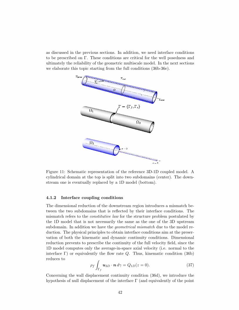
as discussed in the previous sections. In addition, we need interface conditionsto be prescribed on Γ. These conditions are critical for the well posedness andultimately the reliability of the geometric multiscale model. In the next sectionswe elaborate this topic starting from the full conditions (36b-36e).
Figure 11: Schematic representation of the reference 3D-1D coupled model. Acylindrical domain at the top is split into two subdomains (center). The down-stream one is eventually replaced by a 1D model (bottom).
4.1.2 Interface coupling conditions
The dimensional reduction of the downstream region introduces a mismatch be-tween the two subdomains that is reflected by their interface conditions. Themismatch refers to the constitutive law for the structure problem postulated bythe 1D model that is not necessarily the same as the one of the 3D upstreamsubdomain. In addition we have the geometrical mismatch due to the model re-duction. The physical principles to obtain interface conditions aim at the preser-vation of both the kinematic and dynamic continuity conditions. Dimensionalreduction prevents to prescribe the continuity of the full velocity field, since the1D model computes only the average-in-space axial velocity (i.e. normal to theinterface Γ) or equivalently the flow rate Q. Thus, kinematic condition (36b)reduces to
ρf
∫
Γf
u3D · n dγ = Q1D(z = 0). (37)
Concerning the wall displacement continuity condition (36d), we introduce thehypothesis of null displacement of the interface Γ (and equivalently of the point
42
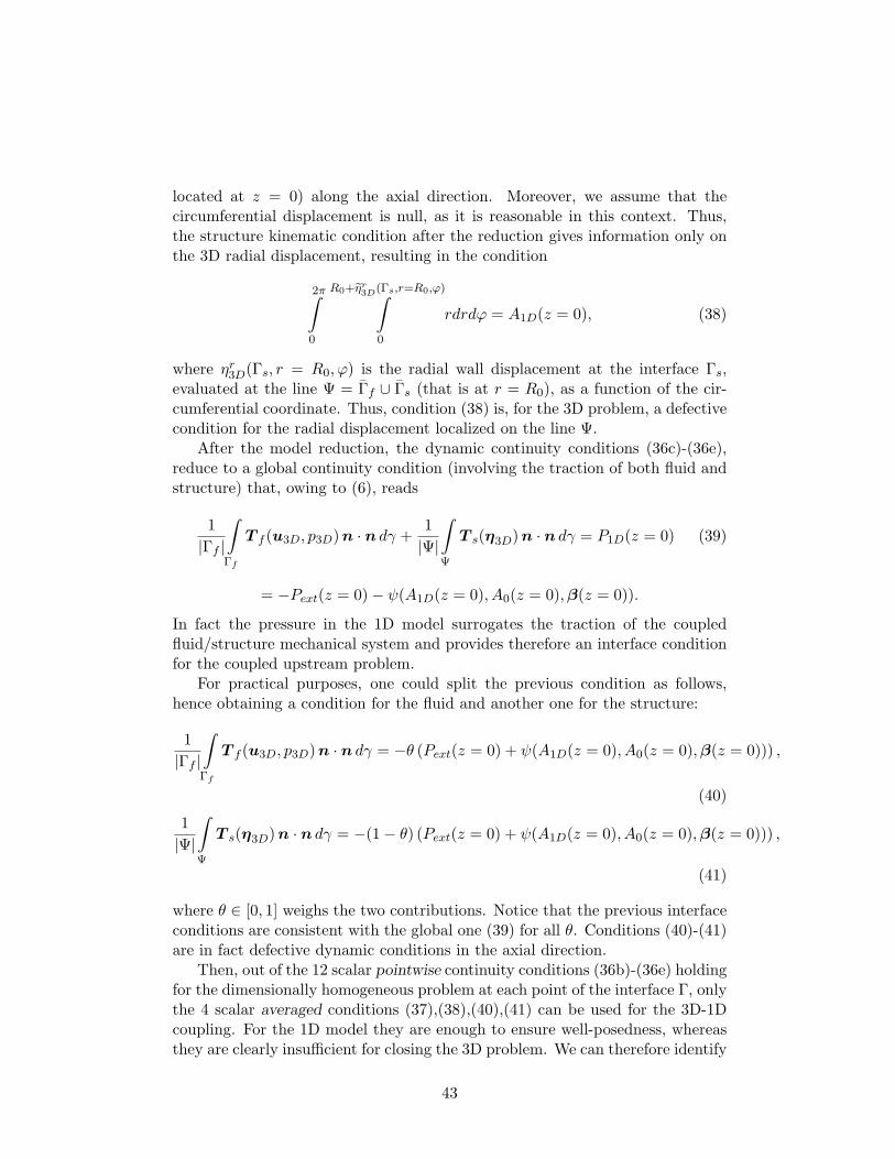
located at z = 0) along the axial direction. Moreover, we assume that thecircumferential displacement is null, as it is reasonable in this context. Thus,the structure kinematic condition after the reduction gives information only onthe 3D radial displacement, resulting in the condition
2π∫
0
R0+ηr3D(Γs,r=R0,ϕ)∫
0
rdrdϕ = A1D(z = 0), (38)
where ηr3D(Γs, r = R0, ϕ) is the radial wall displacement at the interface Γs,evaluated at the line Ψ = Γf ∪ Γs (that is at r = R0), as a function of the cir-cumferential coordinate. Thus, condition (38) is, for the 3D problem, a defectivecondition for the radial displacement localized on the line Ψ.
After the model reduction, the dynamic continuity conditions (36c)-(36e),reduce to a global continuity condition (involving the traction of both fluid andstructure) that, owing to (6), reads
1
|Γf |
∫
Γf
T f (u3D, p3D)n · n dγ +1
|Ψ|
∫
Ψ
T s(η3D)n · n dγ = P1D(z = 0) (39)
= −Pext(z = 0)− ψ(A1D(z = 0), A0(z = 0),β(z = 0)).
In fact the pressure in the 1D model surrogates the traction of the coupledfluid/structure mechanical system and provides therefore an interface conditionfor the coupled upstream problem.
For practical purposes, one could split the previous condition as follows,hence obtaining a condition for the fluid and another one for the structure:
1
|Γf |
∫
Γf
T f (u3D, p3D)n · n dγ = −θ (Pext(z = 0) + ψ(A1D(z = 0), A0(z = 0),β(z = 0))) ,
(40)
1
|Ψ|
∫
Ψ
T s(η3D)n · n dγ = −(1− θ) (Pext(z = 0) + ψ(A1D(z = 0), A0(z = 0),β(z = 0))) ,
(41)
where θ ∈ [0, 1] weighs the two contributions. Notice that the previous interfaceconditions are consistent with the global one (39) for all θ. Conditions (40)-(41)are in fact defective dynamic conditions in the axial direction.
Then, out of the 12 scalar pointwise continuity conditions (36b)-(36e) holdingfor the dimensionally homogeneous problem at each point of the interface Γ, onlythe 4 scalar averaged conditions (37),(38),(40),(41) can be used for the 3D-1Dcoupling. For the 1D model they are enough to ensure well-posedness, whereasthey are clearly insufficient for closing the 3D problem. We can therefore identify
43
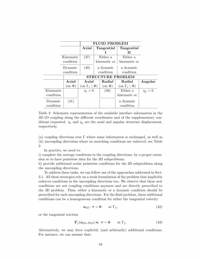
FLUID PROBLEM
Axial Tangential TangentialI II
Kinematic (37) Either a Either acondition kinematic or kinematic or
Dynamic (40) a dynamic a dynamiccondition condition condition
STRUCTURE PROBLEM
Axial Axial Radial Radial Angular(on Ψ) (on Γs \Ψ) (on Ψ) (on Γs \Ψ)
Kinematic ηz = 0 (38) Either a ηϕ = 0condition kinematic or
Dynamic (41) a dynamiccondition condition
Table 2: Schematic representation of the available interface information in the3D-1D coupling along the different coordinates and of the supplementary con-ditions requested. ηz and ηϕ are the axial and angular structure displacement,respectively.
(a) coupling directions over Γ where some information is exchanged, as well as(ii) uncoupling directions where no matching conditions are enforced, see Table2.
In practice, we need to:i) complete the average conditions in the coupling directions, by a proper exten-sion so to have pointwise data for the 3D subproblems;ii) provide additional scalar pointwise conditions for the 3D subproblems alongthe uncoupling directions.
To address these tasks, we can follow one of the approaches addressed in Sect.3.1. All these strategies rely on a weak formulation of the problem that implicitlyenforces conditions in the uncoupling directions too. We observe that these newconditions are not coupling conditions anymore and are directly prescribed tothe 3D problem. Thus, either a kinematic or a dynamic condition should beprescribed for each uncoupling directions. For the fluid problem, these additionalconditions can be a homogeneous condition for either the tangential velocity
u3D · τ = 0 at Γf , (42)
or the tangential traction
T f (u3D, p3D)n · τ = 0 at Γf . (43)
Alternatively, we may force explicitly (and arbitrarily) additional conditions.For instance, we can assume that:
44
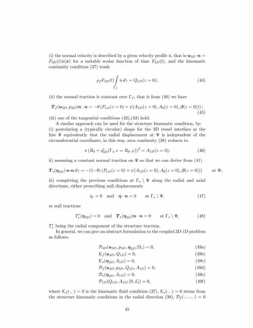
(i) the normal velocity is described by a given velocity profile u, that is u3D ·n =F3D(t)u(x) for a suitable scalar function of time F3D(t), and the kinematiccontinuity condition (37) reads
ρfF3D(t)
∫
Γf
u dγ = Q1D(z = 0); (44)
(ii) the normal traction is constant over Γf , that is from (40) we have
T f (u3D, p3D)n · n = −θ (Pext(z = 0) + ψ(A1D(z = 0), A0(z = 0),β(z = 0))) ;(45)
(iii) one of the tangential conditions (42),(43) hold.A similar approach can be used for the structure kinematic condition, by:
(i) postulating a (typically circular) shape for the 3D vessel interface at theline Ψ equivalently that the radial displacement at Ψ is independent of thecircumferential coordinate; in this way, area continuity (38) reduces to
π (R0 + ηr3D(Γs, r = R0, ϕ))2 = A1D(z = 0); (46)
ii) assuming a constant normal traction on Ψ so that we can derive from (41)
T s(η3D)n·n dγ = −(1−θ) (Pext(z = 0) + ψ(A1D(z = 0), A0(z = 0),β(z = 0))) at Ψ;
iii) completing the previous conditions at Γs \ Ψ along the radial and axialdirections, either prescribing null displacements
ηr = 0 and η · n = 0 at Γs \Ψ, (47)
or null tractions
T rs (η3D) = 0 and T s(η3D)n · n = 0 at Γs \Ψ, (48)
T rs being the radial component of the structure traction.In general, we can give an abstract formulation to the coupled 3D-1D problem
as follows:
P3D(u3D, p3D,η3D; Ω1) = 0, (49a)
Kf (u3D, Q1D) = 0, (49b)
Ks(η3D, A1D) = 0, (49c)
Df (u3D, p3D, Q1D, A1D) = 0, (49d)
Ds(η3D, A1D) = 0, (49e)
P1D(Q1D, A1D; [0, L]) = 0, (49f)
where Kf (·, ·) = 0 is the kinematic fluid condition (37), Ks(·, ·) = 0 stems fromthe structure kinematic conditions in the radial direction (38), Df (·, ·, ·, ·) = 0
45
and Ds(·, ·) = 0 relate to the continuity of the fluid and structure tractions inthe normal direction (40)-(41), and as usual P3D and P1D are abstract represen-tations of the stand-alone 3D and 1D problems, respectively. Different interfaceconditions yield different global problems. The choice of those conditions istherefore critical to guarantee the well posedness (and ultimately the reliability)of the coupled multiscale model. It is therefore important to analyze the prop-erty of energy conservation of every approach and its impact on the physicalconsistency as well as numerical stability.
Remark 6. In the conditions (45)-(46) the area A1D occurs in both the structuredisplacement and fluid traction interface conditions, as a consequence of theconstitutive law in the 1D subproblem. For the 3D problem this may result in anunphysical constraint between the fluid and the structure. In fact, the materialmismatch between the two subproblems - different vessel laws are considered inthe 1D and 3D subproblems - may lead to unreliable results in the 3D domain.A practical cure consists of replacing the kinematic interface conditions for thestructure (such as (46)) by assuming that condition (47) (or alternatively (48))holds true also at Ψ. Using one of these conditions in fact decouples the 3Dstructure and the 1D reduced model. In this case, (49c) reduces to Ks(η3D) = 0.
4.1.3 Energy estimates and interface conditions
For the analysis of the 3D-1D coupled problem, let us assume that the boundaryconditions over the proximal and the distal portions of the boundary of Ω1∪[0, L]and the external side Σext of the 3D domain are homogeneous, i.e.
u3D = 0 at Σf,prox(t), t > 0, (50a)
η3D = 0 at Σs,prox(t), t > 0, (50b)
αST η3D + T s(η3D) n = 0 at Σext, t > 0, (50c)
for the 3D subproblem (we recall that αST is the coefficient accounting for thepresence of surrounding tissues introduced in (3)) and
Q1D = 0 at z = L, (51)
for the 1D one. Moreover, we assume for simplicity Pext = 0.Let us introduce the following total energy for the 3D problem [58, 65]
E3D(t) =ρf2
∫
Ωf
|u3D|2 dΩ+∫
Ωs
ρs2| ˙η3D|2 dΩ+
∫
Ωs
Θ(η3D) dΩ+
∫
Σext
αST |η3D|2dγ
and the following one for the 1D model [58]
E1D(t) =ρf2
∫ L
0A1D u
21D dx+
∫ L
0χ(A1D) dx,
46
where χ(A) =
∫ A
A0
ψ(τ) dτ , ψ being the vessel law (see (6), we outlined its
dependence on A only as it is functional to the estimates we are interestedin), and Θ(η) is the strain energy density function introduced in Section 2.1.Notice that the stand-alone 3D and 1D problems satisfy bounds for this energyfunctionals as proved in [58].
Let Ptot = ψ(A) +ρf2u2 be the total pressure for the 1D model, and ptot in
(29) the total pressure for the 3D model. Then, we have the following resultthat extends the bounds to the multiscale case [65].
Proposition 1. For the interface coupling conditions holding at Γ let us assumethat the following inequality holds
∫
Γf
T f (u3D, ptot,3D)n·u3D dγ+
∫
Γs
T s(η3D)n· ˙η3D dγ+Q1D(z = 0)Ptot,1D(z = 0) ≤ 0.
(52)Then, the coupled 3D-1D problem (1),(7),(50),(51) satisfies the energy decayproperty
d
dt
(E3D(t) + E1D(t)
)≤ 0
for all t > 0.
In particular for inequality (52) to be fulfilled it is sufficient that the interfaceconditions
ρf
∫
Γf
u3D · n dγ = Q1D(z = 0), (53a)
(T f (u3D, ptot,3D)n) |Γf= −Ptot,1D(z = 0)n (53b)
hold for the fluid, together with
T s(η3D)n = 0 at Γs (54)
for the structure [62, 65]. Similarly, inequality (52) holds if relation (54) isreplaced by
η3D · n = 0 at Γs,
(T s(η3D)n)× n = 0 at Γs.(55)
Note that (54) and (55) are in fact independent of the 1D model, resultingin boundary conditions for the 3D structure problems only. This introduces adiscontinuity in the displacement between the 3D and the 1D model.
Instead, conditions
1
|Γf |
∫
Γf
T f (u3D, ptot,3D)n · n dγ = −Ptot,1D(z = 0), (56)
47
or1
|Γf |
∫
Γf
ptot,3D dγ = Ptot,1D(z = 0) (57)
do not guarantee the fulfillment of (52) and thus the energy decay property.Also conditions involving the kinetic pressure (as opposed to the total pres-
sure considered in (56)-(57)) like
1
|Γf |
∫
Γf
T f (u3D, p3D)n · n dγ = −ψ(A1D(z = 0)), (58)
or1
|Γf |
∫
Γf
p3D dγ = ψ(A1D(z = 0)) (59)
do not satisfy condition (52). More precisely, in this case we have
d
dt
(E3D(t) + E1D(t)
)=ρf2
((Q1D(t, z = 0))3
(A1D(t, z = 0))2−∫
Γf
|u3D(t)|2u3D(t) · n dγ).
Even though (theoretically) the right hand side is not necessarily (always) neg-ative [65], numerical evidence suggests that these conditions are actually stable,see [115].
Instead of conditions (58) or (59), in analogy with the general treatment ofthe dynamic conditions provided by (40)-(41), one could also consider a dynamiccondition for the structure, obtaining either
1
|Γf |
∫
Γf
T f (u3D, p3D)n · n dγ = −θψ(A1D(z = 0))
or1
|Γf |
∫
Γf
p3D dγ = θψ(A1D(z = 0)), (60)
in combination with
1
|Ψ|
∫
Ψ
T s(η3D)n · n dγ = −(1− θ)ψ(A1D(z = 0), A0(z = 0),β(z = 0)), (61)
for a suitable θ ∈ [0, 1].
4.1.4 Further developments and comments
Coupling of a 1D model with a 3D rigid model. The arterial pressurewave propagation involves wave lengths typically larger than the size of a do-main to be treated by a full 3D model. This may be troublesome for coupledproblems because on the one hand the physical consistency requires to treatfluid-structure interaction in both the subproblems, however the 3D subproblem
48
is affected by a significant computational burden when FSI is included. De-pending on the applications, it may be reasonable to still approximate the 3Dmodel as a rigid one, in particular when the 1D model is essentially regardedas a physically consistent way of supplying reliable boundary conditions for the3D one. However, this approximation generates a strong discontinuity in theway the wall dynamics is described in the overall problem. This may originatespurious reflections and numerical instabilities at the 3D-1D interface.
A possible remedy has been proposed in [143], by pretending the 3D modelto be compliant at the interface with the 1D submodel by introducing lumpedcompliances. This approach can be interpreted as a 3D-0D-1D coupling, the 0Dbeing the “virtual” portion of the domain where the effects of compliance areintroduced in the model. Alternatively, this modification can be regarded as amodification of the interface conditions between the 3D (only fluid) model andthe 1D one to introduce the effects of compliance. Here, we follow this secondinterpretation. In particular, let us define
P3D =1
|Γf |
∫
Γf
p3D dγ, Q3D = ρf
∫
Γf
u3D · n dγ. (62)
Then, consider the interface conditions
P1D = P3D − LdQ3D
dt−R2Q3D +R1C
dP3D
dt−R1CL
d2P3D
dt2−R1Q3D,
Q3D = Q1D −R1CdQ1D
dt− C
dP1D
dt,
to couple the rigid 3D model to the 1D problem. Here, R1, R2 are two resistances(accounting for viscous effects), L is related to blood inertia and C gathers thecompliance of the 3D model to the interface with the 1D to damp spuriousreflections induced by the structural discontinuity. The cost of the 3D solutionis simply that of a fluid solved in a domain with rigid boundaries. Should wefollow the 3D-0D-1D interpretation of this approach, these conditions stem fromsimple hydraulic network of π type interfacing the two subproblems.
Results presented in [143] show that with an appropriate choice of the param-eters R1, R2, L and C, flow rate and pressure at the systemic level are acceptable,while keeping relatively low computational costs. Yet, choosing the parametersmay be troublesome in patient-specific settings and ad hoc data assimilationprocedures are recommended.
The role of the characteristics for the interface conditions. As we dis-cussed in Sect. 3.2, the 1D problem is strictly hyperbolic and from the mathe-matical standpoint it features two characteristic or Riemann variables propagat-ing in two opposite directions along the 1D domain. Because of the hyperbolicnature of the problem, at the interface with the 3D model it is appropriate theprescription of the Riemann variable that is entering Ω1D. In our example, with
49
the 1D domain located distally to Ω3D, this is W1. For this reason, in practiceone between the pressure or traction interface conditions (53b), (56), (57), (58)or (59) can be replaced by a condition expressing the continuity of W1 [58]. Inparticular, at each time t we may consider condition (53a) and
W1(z = 0) = ζ1 (|Γf |, Q3D) , (64)
with ζ1 given by (32) and Q3D by (62).It is possible to prove that this condition together with (53a) implies the con-
tinuity of the area at the interface while the continuity of the pressure/tractionis not guaranteed.
4.2 3D-0D coupling
4.2.1 Formulation of the problem
In some cases the knowledge of the space dependence of the variables of interestis not crucial in the downstream region Ω2. The dynamics here can be describedby a compartment represented by a lumped parameter model. Following up theoutline of the present section, this case can be regarded as a further simplificationof the 3D-1D model previously considered, where the 1D downstream subdomainis replaced by a 0D description.
Interface conditions between the 3D and the 0D subdomain can be devised byproceeding as done for the 3D-1D case, in particular by prescribing again kine-matic and dynamic continuity conditions, in a form that is adapted to the con-text of the lumped parameter model. For instance, if P3D(u3D, p3D,η3D; Ω1) =0 is the abridged notation for the 3D model (including the inlet conditionson fluid velocity or traction and on structure displacement or traction) andP0D(Q0D, P0D) = 0 represents the downstream lumped parameter model (wherewe highlighted the dependence on the proximal quantities Q0D and P0D), we candevise a set of interface conditions reading as
ρf
∫
Γf
u3D · n dγ = Q0D, (65a)
1
|Γf |
∫
Γf
T f (u3D, p3D)n · n dγ = −θP0D, (65b)
2π∫
0
R0+ηr3D(Γs,r=R0,ϕ)∫
0
rdrdϕ = ψ−1(P0D), (65c)
1
|Ψ|
∫
Ψ
T s(η3D)n · n dγ = −(1− θ)P0D, (65d)
50
where ψ is given by the the algebraic equation (11) relating the area and thepressure and used in the derivation of the 0D model and where again θ ∈ [0, 1].In analogy with the 3D-1D case, we can use for the dynamic fluid continuitya condition like (59) on the mean pressure instead of the normal traction. Asfor the coupling between 3D and 1D models, also in this case the conditions are“defective” for the 3D subdomain and the problem needs to be completed asdone in the previous section.
When coupling 3D with 0D models, three issues need to be enphasized:
1. In the derivation of the 0D model one assumption is that convective termsare in general small. For this reason, the basic derivation for an arterialsegment leads to a linear model, the nonlinear terms having been dropped.Consequently, on the 0D side the pressure coincides with the total pressure,so that a total pressure interface condition simply reads
1
|Γf |
∫
Γf
ptot,3D dγ = P0D.
2. As pointed out in Sect. 2.3, the mathematical formulation of the 0Dmodel does not separate the equations of the dynamics from the “boundaryconditions”; the latter are directly incorporated in the system of ordinarydifferential equations, since the space dependence in the model is dropped.This feature is crucial when devising segregated algorithms for solving the3D-0D problem, since the mathematical representation of the 0D problemhas to be compatible with the associated interface conditions. We willaddress this concept in Section 5.
3. As for the 3D-1D coupling, the mismatch of the structural constitutive lawsseparately postulated in the two subdomains may lead to some spuriousnumerical effects. In this case, often the continuity of the displacement andtractions for the structure problem (65c)-(65d) are dropped and they arereplaced by a homogeneous boundary condition for η3D or for Ts(η3D).
In many applications [202, 102] when coupling 3D and 0D models, the lumpedparameter subdomain is intended to provide just a transfer function to incor-porate the presence of the peripheral impedance into the simulation of the 3Dsubdomain. In this case, the windkessel model and its variants addressed inSect. 2.3.2 provide an excellent simplified description to be embedded straight-forwardly into the solution of the 3D problem. We illustrate a semi-analyticapproach for solving this case in the next subsection.
More generally, coupling between the two models stems genuinely from thenecessity of solving the different scales (local and global) and a windkessel modelis not accurate enough for the level of detail required to the systemic submodel.An example extensively addressed in the literature is given by the numericalmodeling of the Total CavoPulmonary Connection (TCPC), see e.g. [107, 106,
51
121, 83]. In this case, the 0D model - that is in general nonlinear due to thepresence of the valves - is not directly included in the 3D solution; segregatedapproaches are indeed more indicated. This topic will be covered in Section 5.
4.2.2 Monolithic Solution of 3D-0D windkessel models
When the 0D differential system can be formally solved by standard techniquesfor ordinary differential equations, the resulting solutions combine pressure andflow rate to provide a Robin-type defective boundary condition for the 3D fluidproblem.
We illustrate this outcome in the case of the 3-element windkessel peripheralmodels. The extension to the 4-element windkessel models is technically moreinvolved but promptly derived following similar steps.
Let us consider the 3-element windkessel model represented in Fig. 6(b).Referring to the notation reported in the figure, we use here the subscript “0D”to denote quantities related to the lumped parameter model. This model corre-sponds to the differential equation
d(P0D −R1Q0D)
dt+
1
R2C(P0D −R1Q0D) =
Q0D
C.
By a standard application of the method of integrating factors (see e.g. [36]) wefind
P0D(t) = R1Q0D(t)+(P0D(0)−R1Q0D(0)) e−t/(R2C)+
1
C
t∫
0
eτ−t/(R2C)Q0D(τ)dτ.
(66)For the continuity of the normal velocity and of the tractions that we postu-
late at the interface, we setQ0D = ρf
∫
Γf
u3D·n dγ, and P0D = − 1
|Γf |
∫
Γf
T f (u3D, p3D)n·
n dγ. Once plugged in (66), these lead to the following resistance defective con-dition
1
|Γf |
∫
Γf
T f (u3D, p3D)n · n dγ +R1ρf
∫
Γf
u3D · n dγ +ρfC
t∫
0
eτ−t/(R2C)
∫
Γf
u3D(x, τ) · n dγdτ =
1
|Γf |
∫
Γf
T f (u3D(x, 0), p3D(x, 0))n · n dγ +R1ρf
∫
Γf
u3D(x, 0) · n dγ
e−t/(R2C)n.
The previous condition can eventually be incorporated into the variational for-mulation of the Navier-Stokes equations [202].
In practice, in a time-discrete setting for the numerical solution of the prob-lem, (66) is applied over the timeline of the single time step between tn and tn+1,
52
used in combination with a quadrature rule (e.g. the trapezoidal rule) to treatthe third term at the left hand side, leading to
1
|Γf |
∫
Γf
T f (un+13D , pn+1
3D )n · n dγ+ρf (R1+1/2C)
∫
Γf
un+13D ·n dγ = G(un3D, pn3D,u0
3D, p03D),
(67)for a suitable function G of the outlined arguments.
Remark 7. For the practical prescription of condition (67) a possible solutionis given by evaluating the flow rate term through a suitable extrapolation fromprevious time steps, thus leading to a mean traction condition, which could beprescribed, e.g., with the do-nothing approach presented in Sect 3.1.2. This solu-tion is very attractive when one wants to use a commercial solver. In principle,we could follow a dual approach where we extrapolate the mean pressure fromprevious time steps, thus obtaining in fact a flow rate condition. Although possi-ble, this approach requires the treatment of defective flux conditions. As we haveseen in Sect. 3, this is much more complicated, so the previous approach is byfar the most popular.
4.3 1D-0D coupling
At last, we consider the case when a lumped parameter model is coupled to a 1Dmodel in order to include the effects of systemic circulation, for instance whenperipheral circulation is accounted for by means of a suitable boundary conditionto close a 1D model. In this case, the role of the lumped parameter model is tocalculate the pressure wave reflections generated by peripheral districts and bythe microcirculation [63]. In a different context, 0D models have been coupledwith a 1D description of the circulatory network in [61] to include the action ofthe heart.
Coherently with the previous assumptions in the present section, we considerhere the case when a single arterial cylindrical segment is described by a 1Dmodel, proximally in a region Ω1, and by a 0D model in a region Ω2 locateddistally. As done in Sect. 4.1, we start with a split-by-subdomain representationof the same problem in terms of 1D models. Over the segment spanned by theaxial abscissa z ∈ [−L,L] the unsplit 1D problem
P1D(Q1D, A1D, [−L,L]) = 0 (68)
is formulated as the coupling of two 1D subproblems in Ω1 ≡ [−L, 0] and Ω2 ≡[0, L], respectively
P1D
(Q1
1D, A11D, [−L, 0]
)= 0, (69a)
Q11D(z = 0) = Q2
1D(z = 0), (69b)
ψ(A11D(z = 0)) = ψ(A2
1D(z = 0)), (69c)
P1D(Q21D, A
21D, [0, L]) = 0. (69d)
53
Here we have understood convenient conditions at the proximal z = −L anddistal z = L boundaries in the abridged notation P1D(Q
i1D, A
i1D, ·) for i = 1, 2.
In addition, we introduced interface conditions based on the continuity of massand momentum. The latter is written in terms of pressure, regarded as functionof the area Ai1D, i = 1, 2. Other interface conditions can be considered as well,for instance involving the total pressure rather than the pressure. If the functionψ representing the vessel law is the same for the two subproblems, as it is oftenthe case, the continuity of the pressure and that of the flow rates implies thecontinuity of the total pressure. From the mathematical point of view it makessense to consider alternative equivalent interface conditions formulated in termsof characteristic variablesW j
i (Ai1D, Q
i1D), i, j = 1, 2, since they precisely consider
quantities with a well defined direction of propagation.Next, we replace the downstream 1D problem with a suitable 0D model for
a cylindrical segment (and including the appropriate boundary conditions atz = L), leading to the geometric multiscale model
P1D(Q1D, A1D; [−L, 0]) = 0, (70a)
Q1D(z = 0) = Q0D, (70b)
ψ(A1D(z = 0)) = P0D, (70c)
P0D(Q0D, P0D) = 0, (70d)
where again Q0D and P0D represent the proximal quantities in the 0D model.Also in this case, we can replace one of the interface conditions stemming fromthe continuity of mass and momentum with one for the characteristic variableW2
W2(z = 0) = ζ2(ψ−1(P0D), Q0D
), (71)
with ζ2 given by (32). This prevents the occurrence of numerical artifacts in-troduced by approximation errors that trigger unphysical reflections at z = L[63, 56].
In comparison with the 3D-0D case, this coupling is much more intuitive,since both 1D and 0D models compute average area and flow rate over differentpoints of the axis, and no defective conditions need to be sorted out at thecoupling interface. In particular, if the 0D model is simple (like for a cylindricalsegment as well as a windkessel model) a semi-analytical approach based on themethod of integrating factors illustrated in the previous section can be pursued.This means that the pressure P0D can be explicitly computed as a function ofthe flow rate Q0D and used straightforwardly in the prescription of W2.
More in general, when the 0D network is more complicated for the presenceof several compartments and/or nonlinear terms, a partitioned approach has tobe preferred, as we will see in the next Section.
54
5 Numerical strategies
The numerical solution of the coupled geometric multiscale problems presentedin Sect. 4 requires special care. The intrinsic heterogeneity and the diversenature of the problem components drives the set up of a solution algorithm andits analysis. Generally speaking, two basic options can be pursued, a monolithicapproach and a partitioned or segregated one. The latter strategy seems to bemore natural - apart from special cases like the 3D-windkessel coupled modeladdressed in Sect. 4.2.2 - and is discussed in the next subsections.
As for the temporal stability of the solver, this generally follows from therestrictions induced by the time advancing schemes adopted for the differentcomponents of the multiscale model. While implicit or semi-implicit approachesare preferred for the 3D models to avoid stability restrictions of parabolic typein the fluid problem (e.g. the time step ∆t bounded by a quantity scaling withh2), 1D models are usually solved by explicit methods subject to CFL stabilityconditions. General statements on the most restrictive conditions are difficult todraw, as they depend on the specific problem (the vascular district for the 3Dmodel as well as the portion of the network for the 1D one). For this reason, inpartitioned schemes where the different solvers are called in an either sequentialor parallel fashion, it is worth resorting to multi-level time stepping techniques,where the different geometric components are solved with individual convenienttime steps and matching interface conditions are fulfilled thanks to suitablesynchronization procedures [28, 116] - see also Sect. 6.4.2
In the remainder of this Section we keep considering the time discretizationof the coupled problems already introduced in Sect. 4. However, we will dropthe time index n+ 1 for the sake of notation.
5.1 Partitioned algorithms: generalities
A quite natural approach for solving heterogeneous problems is to split theminto their homogeneous components and to delegate iterative schemes to enforcetheir matching. This holds for many applications in multi-physics, and remark-ably for fluid-structure interaction problems [164]. Dimensionally heterogeneousproblems like the ones generated by the geometric multiscale modeling are noexception. As a matter of fact, the intrinsic modularity of this approach per-fectly fits into the need of solving diverse mathematical (and numerical) coupledproblems, including 3D, 1D partial as well as ordinary differential equations [63].
In the previous section, we introduced the sequence (i) domain splitting;(ii) model simplification, to obtain in a systematic way geometric multiscalemodels. Here we bring this procedure to the final step, namely the iterativesubstructuring formulation [164]. This introduces a sequence of dimensionallyhomogeneous problems in the two subdomains, where the interface conditionsiteratively provide boundary data.
When resorting to these domain decomposition techniques, there are basi-
55
cally two fundamental issues to consider at a very general level, namely (a) thewell posedness of each subproblem at every iteration; (b) the convergence of theiterative procedure.
Point (a) in general may be standard when domain decomposition is used asa framework to exploit parallel architectures for solving homogeneous problems.This however is not the case of geometric multiscale models, where the dimen-sional mismatch unavoidably leads to defective boundary problems for the 3Dmodel. The well posedness of the 3D FSI model - at both the continuous andthen at the numerical level - with defective boundary data needs to be carefullyanalyzed - see Sect. 3.1.
Another non-trivial issue arises when considering lumped parameter modelsfor which - as previously pointed out - the concept of boundary data is an abuse,yet physically intuitive, and requires specific adjustments in the formulation ofthe 0D problem. We will address these issues in detail in the next subsections.
As for point (b), we can take advantage of standard techniques for iterativesubstructuring methods, including either sequential block Gauss-Seidel like orparallel block Jacobi like formulations of the algorithm. While it is fairly com-plicated to apply the general theory of iterative schemes to our dimensionallyheterogeneous problems, the gallery of examples in Sect. 6 illustrates successfulschemes for different possible couplings.
It is worth noting that, originally conceived as a numerical solution proce-dure, the partitioned formulation turned out to be an effective tool to investigatewell posedness of geometric multiscale problems, by applying appropriate fixedpoint theorems, as we will specify in Sect. 5.3 [167, 56].
Our exemplifications here will be limited to the simple cylindrical domainintroduced in Sect. 4. For the sake of clarity, we summarize here the notation.With a little abuse we will denote the time-discrete stand-alone models with thesame compact notation used in Section 4 for their time-continuous counterparts.Hence:
- P3D(u3D, p3D,η3D; Ω) = 0 represents the time-discrete 3D problem in theFSI domain Ω with suitable boundary conditions at the fluid and struc-ture inlets and at the physical boundary. The specific time-discretizationscheme used is not important at this stage. At the interface with othersubdomains we postulate conditions like the ones specified in Sect. 4 thatin the framework of partitioned algorithms will provide boundary data.
- P1D(Q1D, A1D; [0, L]) = 0 represents a time-discrete 1D model in the do-main [0, L]. On one side of the domain we will have standard boundaryconditions inherited from the boundary-value problem; on the other one,interface conditions with the corresponding subdomain will provide thenecessary data to solve it as a standard stand-alone problem.
- P0D(S0D) = 0 represents one of the possible problems originating by thetime discretization of the ordinary differential system associated with the
56
networks depicted in Fig. 5, where S0D is the proximal variable (pressureor flow rate) that determine the state of the network.
5.2 The 3D-1D case
Let us consider a partitioned algorithm for the 3D-1D coupled problem. Wespecifically refer to the time discretization of (49) when interface conditionDf (·, ·, ·, ·) = 0 is given by (59), as a special instance of (49d). In Algorithm 1we reported the pseudo-code of this “Flow rate/Mean pressure” scheme whereat each iteration the flow rate computed by the 1D model is used to feed the3D problem as boundary condition for the fluid, whereas the interface meanpressure computed by the 3D problem provides the boundary condition at theinterface with the 1D model [58]. For the sake of exposition we set Pext = 0 andwe do not report explicitly the dependence of A1D on A0 and β.
In Algorithm 1, the kinematic structure condition (49c) has been rewrittenin order for the 1D area at the previous iteration to feed the 3D problem.
Any of the methods illustrated in Section 3.1 can be used to solve the defec-tive 3D problems and compute numerically the 3D fluid velocity and pressureas well as the structure displacement.
As an alternative to Algorithm 1, one could swap the roles of the interfaceconditions, prescribing the mean pressure to the 3D problem and the flow rateto the 1D problem (“Mean pressure/Flow rate” algorithm). In this case at eachiteration we solve a mean pressure defective condition for the 3D problem, withone of the strategies described in Section 3.1. The two schemes, “Flow rate/Meanpressure” and “Mean pressure/Flow rate”, converge to the same solution andthe choice between them is essentially driven by efficiency arguments.
However, there are other possible conditions to be considered for the cou-pling. For instance, interface condition (57) involving the mean total pressurecan replace (59) in Algorithm 1. In this case, the following alternative boundarycondition on the mean pressure for the 1D problem replaces (73b) accordingly
P(k)1D (z = 0) =
1
|Γf |
∫
Γf
p(k)3D dγ +
1
2
1
|Γf |
∫
Γf
|u(k−1)3D |2 dγ −
(Q
(k−1)1D (z = 0)
ρfA(k−1)1D (z = 0)
)2.
This follows from a proper linearization of (57) with a fixed point argumentwithin the same loop used to enforce the fulfillment of the interface conditions[65].
The same conditions can be enforced differently thanks to identity (30) inthe weak formulation of the Navier-Stokes equations and a do-nothing approachas proposed in [62]. In fact, this allows to impose the total pressure as a naturalcondition, thus avoiding subiterations. Since the interface conditions involve thetotal pressure, henceforth differing from the ones considered in Algorithm 1, theconverged solution found will be in general different.
57
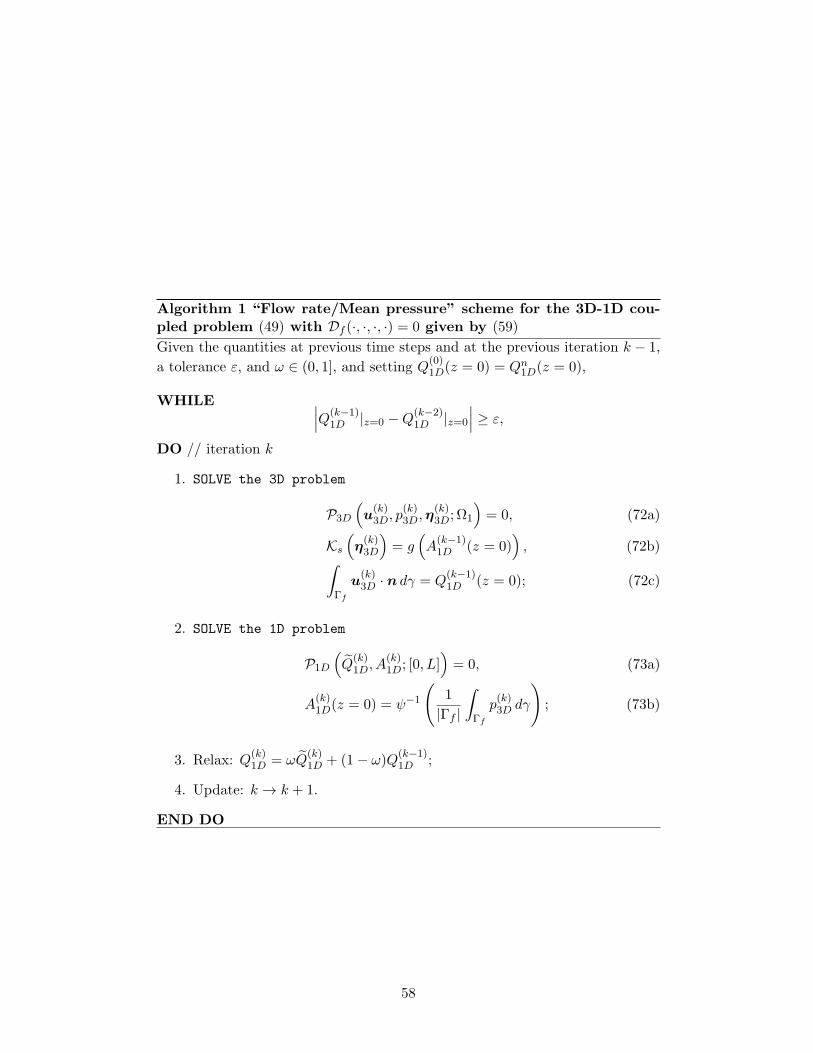
Algorithm 1 “Flow rate/Mean pressure” scheme for the 3D-1D cou-pled problem (49) with Df (·, ·, ·, ·) = 0 given by (59)
Given the quantities at previous time steps and at the previous iteration k − 1,
a tolerance ε, and ω ∈ (0, 1], and setting Q(0)1D(z = 0) = Qn1D(z = 0),
WHILE ∣∣∣Q(k−1)1D |z=0 −Q
(k−2)1D |z=0
∣∣∣ ≥ ε,
DO // iteration k
1. SOLVE the 3D problem
P3D
(u(k)3D, p
(k)3D,η
(k)3D; Ω1
)= 0, (72a)
Ks
(η(k)3D
)= g
(A
(k−1)1D (z = 0)
), (72b)
∫
Γf
u(k)3D · n dγ = Q
(k−1)1D (z = 0); (72c)
2. SOLVE the 1D problem
P1D
(Q
(k)1D, A
(k)1D; [0, L]
)= 0, (73a)
A(k)1D(z = 0) = ψ−1
(1
|Γf |
∫
Γf
p(k)3D dγ
); (73b)
3. Relax: Q(k)1D = ωQ
(k)1D + (1− ω)Q
(k−1)1D ;
4. Update: k → k + 1.
END DO
58
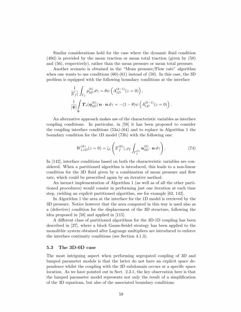
Similar considerations hold for the case where the dynamic fluid condition(49d) is provided by the mean traction or mean total traction (given by (58)and (56), respectively), rather than the mean pressure or mean total pressure.
Another scenario is obtained in the “Mean pressure/Flow rate” algorithmwhen one wants to use conditions (60)-(61) instead of (59). In this case, the 3Dproblem is equipped with the following boundary conditions at the interface
1
|Γf |
∫
Γf
p(k)3D dγ = θψ
(A
(k−1)1D (z = 0)
),
1
|Ψ|
∫
Ψ
T s(η(k)3D)n · n dγ = −(1− θ)ψ
(A
(k−1)1D (z = 0)
).
An alternative approach makes use of the characteristic variables as interfacecoupling conditions. In particular, in [58] it has been proposed to considerthe coupling interface conditions (53a)-(64) and to replace in Algorithm 1 theboundary condition for the 1D model (73b) with the following one:
W(k)1,1D(z = 0) = ζ1
(|Γ(k)f |, ρf
∫
Γ(k)f
u(k)3D · n dγ
). (74)
In [142], interface conditions based on both the characteristic variables are con-sidered. When a partitioned algorithm is introduced, this leads to a non-linearcondition for the 3D fluid given by a combination of mean pressure and flowrate, which could be prescribed again by an iterative method.
An inexact implementation of Algorithm 1 (as well as of all the other parti-tioned procedures) would consist in performing just one iteration at each timestep, yielding an explicit partitioned algorithm, see for example [62, 142].
In Algorithm 1 the area at the interface for the 1D model is retrieved by the3D pressure. Notice however that the area computed in this way is used also asa (defective) condition for the displacement of the 3D structure, following theidea proposed in [58] and applied in [115].
A different class of partitioned algorithms for the 3D-1D coupling has beendescribed in [27], where a block Gauss-Seidel strategy has been applied to themonolithic system obtained after Lagrange multipliers are introduced to enforcethe interface continuity conditions (see Section 4.1.3).
5.3 The 3D-0D case
The most intriguing aspect when performing segregated coupling of 3D andlumped parameter models is that the latter do not have an explicit space de-pendence whilst the coupling with the 3D subdomain occurs at a specific spacelocation. As we have pointed out in Sect. 2.3.1, the key observation here is thatthe lumped parameter model represents not only the result of a simplificationof the 3D equations, but also of the associated boundary conditions.
59
For a model retaining space dependence (either 3D or 1D), different data canbe prescribed at the boundary. Conversely, the specific formulation of a lumpedparameter model of a cylindrical compliant pipe depends on the data prescribedto force its dynamics (see Fig. 5). The portion of the lumped parameter modelreceiving this input reflects the nature of the data. This leads to the concept ofbridging region [167].
The bridging region is an abstract concept to identify the transition betweenthe region occupied by the 3D model and the “region” where the 0D model holds.In fact, it is functionally surrogated by an ODE that makes this transition math-ematically correct. The word “correct” refers to the compatibility between theinterface conditions that in the segregated algorithm are eventually associatedwith the subdomains and the surrogate model that governs the transition in the0D region.
For instance, pressure input data for the 0D model will require a bridgingregion for the computation of the flow rates. This bridging region in fact inter-acts with the 3D model through an inductive term, representing a differentialequation for the flow rate. Similarly, flow rate input data call for the pressure atthe interface as state variable. This means that the bridging region, mathemat-ically represented by a differential equation for the pressure, will be representedby a compliance term (see Fig. 5.3).
On the contrary, if we prescribe a pressure (or a flow rate) to feed a compliant(or inertial) region, the dynamic of the pressure (flow rate) there does not needto be computed; the mathematical model of the hydraulic network features adifferential equation for pressure (flow rate) and it is thus redundant. It may beconveniently reduced (by eliminating the redundant component) to solve it.
More in general, we say that we have the bridging region compatibility if thedata that feed the lumped parameter model are consistent, in the sense thatthey generate no redundancy in the hydraulic network.
This connection between input data and network topology has a central rolewhen devising partitioned algorithms. In fact, when we segregate the computa-tion of the different subdomains, the interface conditions are iteratively associ-ated with the subproblems as boundary data. In non-overlapping partitions, wehave different conditions (Dirichlet/Neumann, Robin/Robin, etc.) to associatewith the different subdomains. For dimensionally heterogeneous models involv-ing a 0D subdomain, the selected boundary condition acts as forcing term forthe lumped parameter system. Under bridging region compatibility the natureof this forcing term dictates then the topology of the network. We illustrate thisconcept in Fig. 5.3. If we associate flow rate conditions to the 0D system thenthe compatible bridging region will have a compliance term (capacitance) at theinlet. Similarly, bridging region compatibility implies that pressure input findsan inertial term (inductance) at the “entrance” of the 0D subdomain. Algorithm2 illustrates a simple instance of this scenario. More precisely, we consider thecoupled problem 3D-0D with interface conditions (65). In this case, the flowrate condition (65a) requires a compatible bridging region like a L or π network,
60
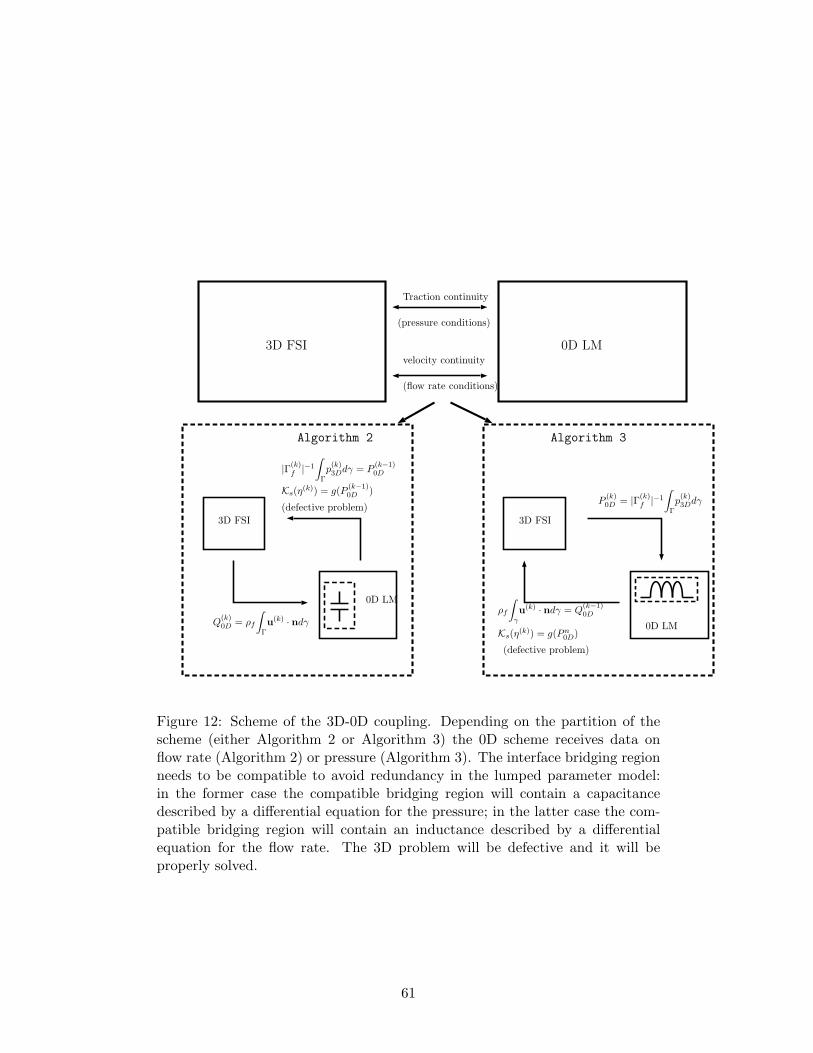
0D LM
(defective problem)
ρf
∫
γu(k) · ndγ = Q
(k−1)0D
P(k)0D = |Γ(k)
f |−1
∫
Γp(k)3Ddγ
3D FSI
0D LM
Q(k)0D = ρf
∫
Γu(k) · ndγ
(defective problem)
|Γ(k)f |−1
∫
Γp(k)3Ddγ = P
(k−1)0D
3D FSI
Algorithm 2 Algorithm 3
Ks(η(k)) = g(Pn0D)
Ks(η(k)) = g(P
(k−1)0D )
Traction continuity
velocity continuity
(pressure conditions)
(flow rate conditions)
3D FSI 0D LM
Figure 12: Scheme of the 3D-0D coupling. Depending on the partition of thescheme (either Algorithm 2 or Algorithm 3) the 0D scheme receives data onflow rate (Algorithm 2) or pressure (Algorithm 3). The interface bridging regionneeds to be compatible to avoid redundancy in the lumped parameter model:in the former case the compatible bridging region will contain a capacitancedescribed by a differential equation for the pressure; in the latter case the com-patible bridging region will contain an inductance described by a differentialequation for the flow rate. The 3D problem will be defective and it will beproperly solved.
61
that links the 3D with a compliance term. On the 3D side, the data retrievediteratively from the lumped parameter model are clearly defective. The meanpressure 3D for the fluid may be completed with the “do-nothing” approachconverting pressure data to natural Neumann conditions on the tractions. Infact, the pressure and the area are related by an algebraic law, so that once oneis computed the other is promptly recovered. In particular, area retrieved fromthe lumped parameter model may be used to prescribe a defective structuredisplacement for the 3D problem (see Sect. 3.1.4). In an oversimplified setting,displacement may be simply set to zero, as we discussed in the Remark 6.
In Algorithm 2 we use a strongly or implicit coupling iterative procedure.The different problems are iteratively solved within each time step up to thefulfillment of the chosen convergence criterion. The mean pressure is prescribedto the 3D model as a mean pressure condition. Again, a condition on the meannormal traction or on the mean total pressure could be considered as well. Asfor the 3D-1D coupling, an explicit variant performs just one iteration per timestep. This is based on a time extrapolation argument of interface variables. Forinstance, in Algorithm 2 we may perform at each time step tn+1 just one iterationby using as initial guess the pressure retrieved at time tn as boundary conditionfor the 3D fluid problem. The rationale is that Pn0D is a first order approximationof Pn+1
0D with respect to ∆t. This time extrapolation (or similar with higher orderdependence on the time step) generally introduces a stability limitation to thetime step that may adversely impact the computational advantage of not solvingthe subproblems several times at each time step - see [161]. We call this secondapproach weakly or loosely coupled.
In Algorithm 3 we illustrate the “dual” case where pressure data are pre-scribed to the 0D model interfacing with an inductive bridging region, like theone for instance of a L−inverted or T network (see Fig. 5). Correspondingly,the 3D fluid model receives flow rate prescribed for instance by a Lagrange mul-tiplier approach (see Sect. 3.1). Other approaches for this are possible as well.As for the 3D structure, area condition are prescribed by properly extrapolat-ing data from the previous iterations/time steps. Again, simplified coupling isoften performed by prescribing null displacement in the axial direction and nulltraction in the tangential directions.
An example of application of Algorithm 3 (for a 3D problem with rigidboundary) is reported in [195].
The convergence of these schemes can be proven by means of general ab-stract arguments for iterative methods. Let F be the abstract notation for thedifferential operator related to a suitable linearization of the fluid-structure 3Dproblem P3D = 0 operating on the variables v3D. Correspondingly, B representsthe action of the variables of the lumped parameter models v0D so that at eachtime step P3D = 0 can be rewritten in the generic form
Fv3D + Bv0D = b3D,
where b3D collects the effect of forcing terms, time discretization terms, bound-
62
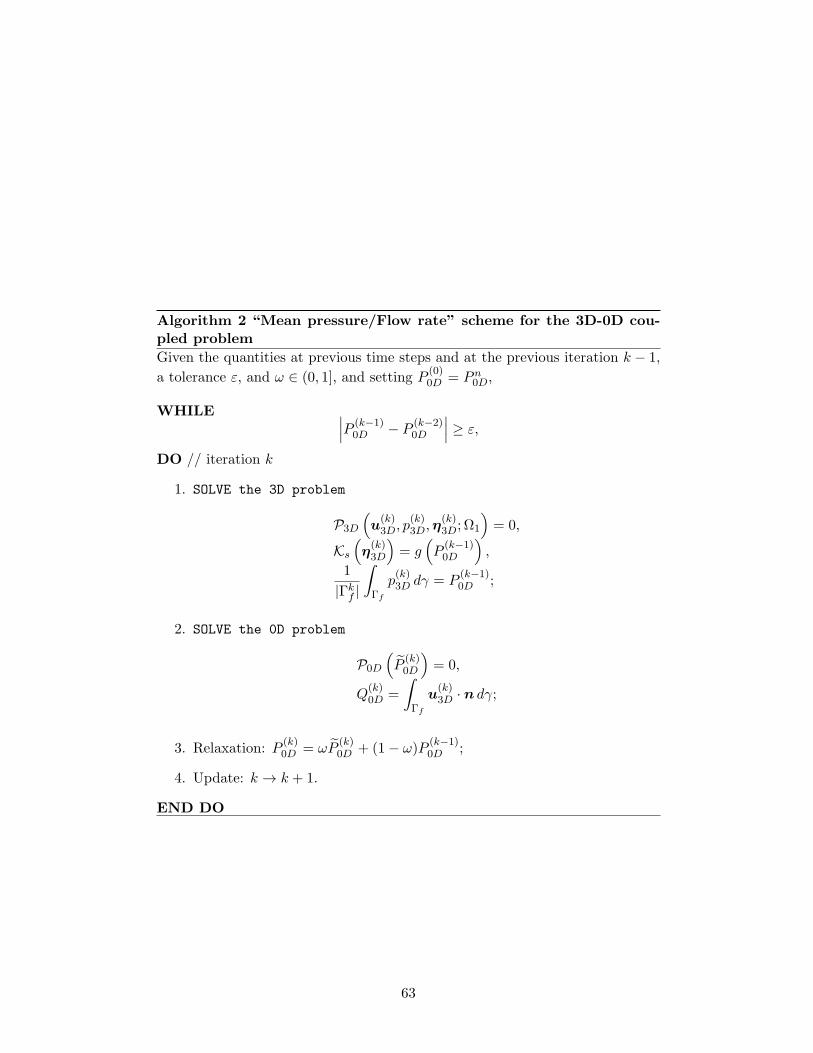
Algorithm 2 “Mean pressure/Flow rate” scheme for the 3D-0D cou-pled problem
Given the quantities at previous time steps and at the previous iteration k − 1,
a tolerance ε, and ω ∈ (0, 1], and setting P(0)0D = Pn0D,
WHILE ∣∣∣P (k−1)0D − P
(k−2)0D
∣∣∣ ≥ ε,
DO // iteration k
1. SOLVE the 3D problem
P3D
(u(k)3D, p
(k)3D,η
(k)3D; Ω1
)= 0,
Ks
(η(k)3D
)= g
(P
(k−1)0D
),
1
|Γkf |
∫
Γf
p(k)3D dγ = P
(k−1)0D ;
2. SOLVE the 0D problem
P0D
(P
(k)0D
)= 0,
Q(k)0D =
∫
Γf
u(k)3D · n dγ;
3. Relaxation: P(k)0D = ωP
(k)0D + (1− ω)P
(k−1)0D ;
4. Update: k → k + 1.
END DO
63
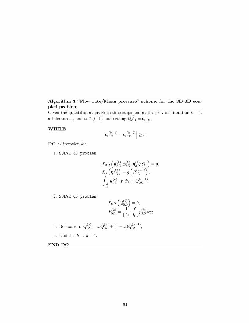
Algorithm 3 “Flow rate/Mean pressure” scheme for the 3D-0D cou-pled problem
Given the quantities at previous time steps and at the previous iteration k − 1,
a tolerance ε, and ω ∈ (0, 1], and setting Q(0)0D = Qn0D,
WHILE ∣∣∣Q(k−1)0D −Q
(k−2)0D
∣∣∣ ≥ ε,
DO // iteration k :
1. SOLVE 3D problem
P3D
(u(k)3D, p
(k)3D,η
(k)3D; Ω1
)= 0,
Ks
(η(k)3D
)= g
(P
(k−1)0D
),∫
Γkf
u(k)3D · n dγ = Q
(k−1)0D ;
2. SOLVE 0D problem
P0D
(Q
(k)0D
)= 0,
P(k)0D =
1
|Γf |
∫
Γf
p(k)3D dγ;
3. Relaxation: Q(k)0D = ωQ
(k)0D + (1− ω)Q
(k−1)0D ;
4. Update: k → k + 1.
END DO
64
ary data (with the exclusion of the interface variables) and time discretization.Similarly, we rewrite P0D = 0 in the form
Lv0D +Dv3D = b0D,
where L is the differential system of the lumped parameter model, D representsthe action of the interface variables computed by the linearized 3D model, andb0D collects the external forcing and time discretization terms.
After appropriate discretization and linearization procedures, the multiscalemodel can be therefore written in the matrix like formulation
[F BD L
] [v3D
v0D
]=
[b3D
b0D
].
In this respect, the iterative methods illustrated in Algorithm 2 and 3 can beregarded as block relaxed Gauss-Seidel schemes. As a matter of fact, if we definethe operator L0D ≡ L−1D and L3D ≡ F−1B, then the relaxed Gauss-Seidelmethod can be formulated as
v(k+1)0D = [(1− ω)I + ωL0DL3D]v
(k)0D + f
(k)0D ,
for a suitable vector f(k)0D . In principle, convergence can be guaranteed by prov-
ing that for an appropriate choice of the relaxation parameter ω the operator[(1− ω)I + ωL0DL3D] is a contraction. In practice, it is fairly difficult to findan explicit formula for ω (generally dependent on the discretization parameters)and a trial and error approach is used. The previous analysis holds also for the3D-1D coupling. In this case, the dependence of the optimal ω on the physicalparameters of the problem has been numerically investigated in [58] .
Robin/Robin interface conditions. In the examples above we have consid-ered interface conditions involving pressure and velocity (converted in averagepressures and flow rates for the 0D) separately. As for Domain Decompositionmethods, this corresponds to selecting Dirichlet/Neumann schemes, where thevelocity conditions represent Dirichlet conditions and the pressure the Neumannones. Other conditions can be equivalently considered, for instance Robin/Robinconditions stemming from a linear combination of the Dirichlet/Neumann ones.From the standpoint of the continuous - dimensionally homogeneous - problem,all these choices are equivalent. The only requisite is that the two selected condi-tions are linearly independent one of the other. Conversely, from the standpointof the approximation, the different conditions will generally lead to different nu-merical sequences (all sharing the same limit, though) and, most importantly,to different numerical performances. An appropriate selection of the param-eters of the combination is in fact expected to accelerate the convergence ofthe partitioned scheme. We observe that for the hydraulic network topology,Robin conditions correspond to introducing a lumped resistance on the interface
65
branch of the bridging region. This case has been considered in [167]. Instead,for the 3D problem, the Robin/Robin scheme would lead to a defective resistancecondition (see (27) and the related paragraph).
Remark 8. Failing to fulfill the bridging region compatibility may introducesome troubles in the segregated algorithm. In fact, if the redundancy of the 0Dmodel is not properly managed, the solution of the 0D compartment may sufferfrom numerical instabilities that affect the convergence of the partitioned scheme.This is illustrated in the counterexample reported in the Appendix of [125].
Remark 9. The original basic iterative scheme can be generalized for the sake ofnumerical efficiency in several ways. For instance, in [22] the partitioning of thegeometrical multiscale model is combined with a fractional step method for solvingthe fluid problem, so that the dimensional mismatch at the interface affects onlyone substep of the 3D problem with a global mitigation of the numerical effectsof the mathematical heterogeneity of the two subproblems.
Segregated schemes as a well posedness fixed point analysis tool. Asfor the theoretical aspects pointed out in the introduction to this section, bridg-ing region compatibility is relevant to ensure the well posedness of each sub-domain problem. In fact, in terms of network analysis it guarantees that thesimple State Variable solution approach described in [104] can be pursued, sinceit implies the absence of capacitance loops and inductance cut sets. In mathe-matical terms, 0D models are described by Differential Algebraic Systems (DAE)of equations and bridging region compatibility guarantees that the system is oftype 1 [6], so it reduces to a standard system of ODE. On the other hand, thedefective 3D problem may be completed as illustrated above (and previouslyin Sect. 3.1). Assuming therefore that also the 3D problem is well posed, theiterative procedure explained in the algorithms above can be used not only forachieving the numerical solution of the coupled problem, but also for proving itswell posedness. As a matter of fact, the coupled solution may be regarded as thefixed point of the iterative scheme. In this perspective, existence (at least locallyin time) follows from the application of fixed point theorems. In particular, inProposition 5.1 of [167] the Schauder fixed point principle was used to analyzethe case of 3D problem with rigid boundaries, after showing that (i) for suitableassumptions on the initial data and under bridging region compatibility, eachsubproblem is well posed; at the numerical level, this implies that the the blockoperators L and F are invertible; (ii) the operator T = L0DL3D is locally-in-time compact. In particular, the proposition was proved for a problem whereall the data used as input to the 0D model where flow rates and the bound-ary conditions for the 3D one were of (defective) pressure types completed withthe “do-nothing” approach. The arguments may be generalized to other casesthough, see [56].
66
5.4 The 1D-0D case
We discuss here about partitioned algorithms related to the time discretizatonof the 1D-0D coupled problem introduced in Section 4.3, which is formally givenby (70). These algorithms are based on the iterative exchange of the interfaceconditions between the 1D and the 0D models. Again, the concept of bridgingregion should be carefully addressed since the 0D model beckons one of the twointerface conditions. In particular, for the solution of (70) a “Pressure/Flowrate” scheme like the one reported in Algorithm 2 could be considered, wherethe pressure condition (70c) is prescribed to the 1D model and the flow ratecondition (70b) to the 0D model. Viceversa, a “Flow rate/Pressure” schemesimilar to the one reported in Algorithm 3 could be considered as well.
An explicit version of “Pressure/Flow rate” algorithm has been used in [56].Instead, a condition on the incoming characteristic variable for the 1D model toreplace the one on the pressure has been proposed in [63].
It is worth mentioning that - similarly to the 3D-0D case - a partitionedapproach has also provided the framework for the well posedness analysis of thisheterogeneous problem via the application of a fixed point theorem, as illustratedin [56].
5.5 Further developments and comments
The partitioned strategies presented in the previous subsections arise from suit-able iterative methods (such as the block Gauss-Seidel method) applied to the“monolithic” coupled problems. A different approach to solve the coupled prob-lems presented in Section 4 relies on writing an equation involving only theinterface unknowns and on its iterative numerical solution (possibly after a suit-able linearization). We can interpret this interface equation as the geometricheterogeneous counterpart of the Schur complement equation, often consideredin the Domain Decomposition method [164].
In [110], a non-linear system of equations involving the interface unknownsrelated to the pressure and the flow rate has been derived for a general networkcomposed by “complex” (3D or 2D) and “simple” (1D or 0D) models, with anarbitrary connectivity. Then, the authors proposed to apply to this interfaceequation either the Broyden method or the Newton one used in combinationwith GMRes - see also Sect. 6.4.2.
A similar strategy has been considered in [115], where the authors detailedthe computation of the Jacobian entries (or of suitable approximations) relatedto the application of the Newton method to the interface equation. The sameframework has been applied in [26] to an interface equation related to flow ratesand total pressure.
The methods derived from an interface equation are particular suited in thecase on multiple interfaces, such as those that arise in complex arterial networksbecause of their simplicity. As a matter of fact, they deal with arrays that
67
corresponds to a lower dimensional space (single points) yielding therefore asubstantial topological simplification.
Finally, we stress again that segregated algorithms are not the only option.Iterative methods applied directly to the monolithic coupled linearized systemhave been advocated in [27, 29].
6 An annotated review of selected works
In this section, we review some of the most-representative contributions to thegeometric multiscale approach in the past fifteen years. For several possiblecoupling problems (3D-1D, 3D-0D, 1D-0D or 3D-1D-0D), we chose two papers,the former with a more theoretical focus on numerical algorithms and theirperformances; the latter more oriented to practical aspects and applications. Inthis choice we necessarily had to discard many contributions. We tried howeverto give an exhaustive outlook to the available literature in the previous sections.
6.1 3D-1D coupling
6.1.1 “On the coupling of 3D and 1D Navier-Stokes equations forflow problems in compliant vessels”, by L. Formaggia, J.F.Gerbeau, F. Nobile, A. Quarteroni, 2001 [58]
The coupling 3D/FSI -1D models is addressed for the first time in [58], where cru-cial mathematical and numerical topics are elucidated and problematic aspects -still open and debated - are highlighted. In particular, the authors consider thecoupling between a 3D/FSI problem with the membrane structure (5) and a 1Dmodel with the algebraic vessel law (11). Energy estimates for the stand-alone3D/FSI and 1D models are provided. For the 3D/FSI problem, the authors de-rive the energy estimate for different boundary conditions on the structure at theoutlet. They consider in particular the case of absorbing boundary conditionsfor the structure, an effective tool to avoid spurious reflections. Referring to thenotation of Section 2.1.3 and to Figure 11, this outlet condition reads
∂ηr∂t
−√kGHs
ρs
∂ηr∂z
= 0. at Σs,dist.
The estimates for the stand-alone models provide the starting point for provingthe global energy estimate reported here in Proposition 1.
For the numerical simulations, the authors resort to a partitioned algorithm(see Algorithm 1). More precisely, mean traction condition (58) is prescribed tothe the 3D fluid problem, whilst 1D model is equipped with condition (74) onthe incoming characteristic variable.
Results are presented both in 2D and 3D cylindrical domains with differentradii and a proximal pressure impluse triggering the dynamics.
68
Hereafter, we report the main results highlighted by the numerical experi-ments.
- An explicit partitioned algorithm manages the 3D-1D coupling with stableresults in the simplified settings tested.
- Condition (72b) to guarantee the continuity of the area (38) at the in-terface leads to numerical instabilities. Most likely this follows form themismatch of the structure laws of the 3D/FSI and 1D models. This con-dition was then replaced by homogeneous Dirichlet condition in the axialdirection and homogeneous Neumann conditions in the tangential one forthe structure.
- Both in the 2D and in the 3D experiments, the stand-alone 3D/FSI modelwith standard outlet boundary conditions exhibits remarkable spurious re-flections. Conversely, these reflections are highly damped in the multiscale3D/FSI-1D model.
- In order to assess the consistency of the geometric multiscale model withthe full high-fidelity one, the authors compare the results of a 2D/FSI sim-ulation and the companion 2D/FSI-1D multiscale model where the distalhalf of the domain is replaced by a 1D system. Results pinpoint that thetwo models are in good agreement until the pressure wave reaches the in-terface between 2D and 1D subdomains (velocity and pressure mismatchin the L2 norm being less than 2.5% and 1.5% respectively). The assess-ment of this consistency is clearly crucial for the reliability of the results.For this reason, this topic has been successively addressed for the case ofa thick structure, in [62] for the case of a cylindrical domain, and in [65]for the case of real geometries. In the latter work, the authors stress theimportance of accounting for the variations of A0 along z in the 1D model(that is ∂A0
∂z 6= 0 in (8b), as we have for instance for stenoses or for tapering
- in this latter case ∂A0∂z ≤ 0) in order to guarantee the consistency.
6.1.2 ‘On the potentialities of 3d-1d coupled models in hemodynam-ics simulations” by P.J. Blanco, M.R. Pivello, S.A. Urquiza,R.A. Feijoo, 2009 [29]
The authors investigate here the consistency of the 3D/FSI-1D coupled systemin real geometries with a circulatory network represented by a system of 1Dproblems. In particular they consider the 55 arteries-network proposed in [7].Each segment is assumed to obey the algebraic vessel law (11). A 3D/FSIproblem with the membrane structure law (5) replaces different portions of thenetwork in the different experiments An implicit partitioned scheme with 3 to 6iterations per time step is exploited.
We report the main results highlighted by the numerical experiments.
69
- The first numerical experiment is intended to analyze numerically the im-pact of the location of the 1D segment replaced by the 3D/FSI model inthe multiscale setting. For this reason, three cases are considered: (i) the3D region Afull replaces a significant portion of the femoral artery; (ii) the3D region Aprox replaces only the first proximal part of the same artery;(iii) the 3D region Adist replaces only the distal tract of the same artery. Inparticular, the two latter domains are selected in such a way that Adist isan almost rectilinear morphology as opposed to Aprox that is significantlycurved. The three multiscale problems are eventually tested against thefull 1D stand-alone model. Results are in good agreement as for the aver-age flow and pressure. In addition, pointwise velocity in the high fidelitymodels is much more similar in the multiscale problems Afull and Aprox
than for the fully 1D and the multiscale with Adist. This because the basic1D model postulates a rectilinear segment - as seen in Sect. 2 - so thecurvature of the femoral artery is not included in the last two cases as itis in the former two, and this significant affects the numerical results.
- In the second test, the authors compare the 1D network with a 3D/FSI-1D,where the high-fidelity model is used to represent the left carotid artery.The aim is to assess te sensitivity of the 3D solution to the inflow conditionsprescribed at the heart. Four typical flow waveform characterizing the flowentering the ascending aorta are employed. The results show that whilethese conditions have a major impact on the systemic 1D solution, thelocal solution in the 3D model (including the wall shear stress) is quiteinsensitive to the different waveforms.
6.2 3D-0D coupling
6.2.1 “Coupling between lumped and distributed models for bloodflow problems” by A. Quarteroni, S. Ragni and A. Veneziani,2001 [161]
As we mentioned in Sect. 1, the interplay between local and systemic dynamicsin determining the boundary conditions for a numerical simulation was well ev-ident before mathematical multiscale models were developed. In fact, in [147] a3D rigid simulation of the cavopulmonary anastomosis was assisted by a lumpedparameter model. The latter was a lumped parameter network covering the en-tire circulation with the role of finding boundary data to be properly prescribedto the stand-alone restricted 3D model of the region of interest. Two separatesolvers were used in this way to improve the reliability of the accurate 3D simula-tion as opposed to the seminal paper [161]. The latter provides the first exampleof a mathematically sound coupled model, where a rigid Navier-Stokes code anda lumped parameter solver defined on non-overlapping regions work in a trulymultiscale fashion. At this proof-of-concept stage the full solver is actually in2D, since a customized research software developed by the authors was used.
70
The conceptual scheme for multiscale modeling is not however affected by thisfact and the paper illustrates results when the systemic network has a certainlevel of complexity, including modeling of the heart and the valves. In partic-ular, the strategy is to segregate the computation in the two subdomains (2Dand 0D) with an explicit time advancing. More precisely, given all the velocityand pressure quantities at a given time step,
1. the solution of the lumped parameter model is computed by using the fullvelocity available from the previous time step, averaged along the interfaceand acting as a forcing term; this obtains the average pressure at theinterface;
2. the latter is used as boundary condition for the 2D problem. More pre-cisely, the related 2D Navier-Stokes pressure drop problem is solved withthe “do-nothing” approach; the nonlinear convective term is approximatedwith a semi-implicit approach.
This completes the multiscale coupling step at a given instant and the time loopmoves forward (see Algorithm 5.2 for the version of this algorithm correspondingto the FSI problem).
Notice that the topology of the lumped parameter solver is selected to be”bridging region compatible”, having capacitance at the interfaces, with pressurerepresenting a state variable for the ODE solver.
The paper presents an algebraic formulation of both the explicit and implicitformulation - based on subiterations between the two solvers at each time step.The time step is selected to guarantee stability to the semi-implicit Navier-Stokessolver. In the simplified test cases considered, the explicit solver is overall stable.
The effectiveness of the multiscale segregated solver is assessed in differenttests. A first test compares the results in a 2D pipe region with the pressure dropprescribed by the network with the available relative Womersley solution, prov-ing the consistency of the multiscale solution with the analytical one. Similarly,the consistency between the solution of the lumped parameter multiscale solverand a stand-alone lumped parameter systemic model is tested, showing that themultiscale model succeeds in providing accurate results in a region of interest,yet preserving an excellent quantitative assessment of the systemic circulation.
As preliminary nontrivial results, the solver is then tested on a simplifiedcoronary by-pass anastomosis test case. The test points out the importance ofa genuine multiscale modeling to capture the local and global different hemody-namics triggered by different morphological (even if simplified) features.
In spite of its simplicity, this paper provides the basis for many multiscalemodels relying on segregated schemes in more realistic contexts. In this respect,we mention [107, 106, 121] applied to the Total Cavopulmonary Connection ob-tained as a therapy for Left Ventricle Hypoplasia Syndrome and [12] for theanalysis of carotid stenosis. In the latter paper, an extensive comparison of dif-ferent boundary conditions in both stand-alone and multiscale settings is carried
71
out, pointing out the importance of the combination of local/systemic perspec-tives granted by multiscale coupling for the reliability of numerical simulations.
More recently, an implicit segregated solver is used in [125] for a detailedanalysis of the Cavopulmonary Connection. The paper points out the nega-tive impact that may have the violation of bridging region compatibility on thestability of the numerical solver.
6.2.2 “On Coupling a Lumped Parameter Heart Model and a Three-Dimensional Finite Element Aorta Model” by H. Kim, I.E.Vignon-Clementel, C. Figueroa, J. Ladisa, K. Jansen, J. Fein-stein, and C. Taylor, 2009 [102]
Paper [102] presents a sophisticated implementation of the 3D-0D coupling forthe reliable simulation of the aortic flow including a simplified model of the heart.The approach followed by the authors in this case is an instance of the “coupledmultidomain method” introduced in [202]. As pointed out in Sect. 4.2.2, this ismonolithic coupling of the 3D and the 0D model. The 0D model at the outflowis actually a 3-element windkessel. As we have seen, a semi-analytical solutionof the network is available thanks to the method of integrating factor. This isincluded in the variational formulation of the Navier-Stokes equation. In thespirit of the “do-nothing” approach indicated in [87], the selected variationalformulation automatically includes the 0D available solution and enforces theinterface conditions filling the gap between the 3D and 0D models.
A distinctive feature of the paper is the inclusion of the heart dynamicsrepresented by a 0D model as well. A similar procedure was carried out in [61]with a 1D-0D coupling to cover the 55 largest arteries represented by 1D modelsdynamically interfaced with the left ventricle (0D). In particular, the nature ofthe boundary conditions for the 3D model at the interface with the heart areselected differently over the heart beat,
1. pressure conditions with the coupled multidomain method are prescribedwhen the valve is open;
2. homogeneous Dirichlet conditions are prescribed when the valve is closed.
With “pressure conditions” we mean here again the inclusion in the Navier-Stokes variational formulation of data on the average pressure provided by anelastance-varying model for the ventricle. The switch of the valve between thetwo possible conditions is governed by
- the difference between the ventricular and the aortic pressures to changefrom close to open: when the ventricular pressure is greater than the aorticone, the type of boundary condition changes;
- the flow rate to change from open to close: when the flow at the interfacebecomes retrograde, the type of the prescribed conditions changes.
72
The model is applied to patient-specific aortic geometries. The detailed3D model includes a linearly elastic deformable wall. Several simulations werecarried out testing the multiscale solver under different conditions
1. rest vs exercise conditions, by reducing the downstream resistances (corre-sponding to vessel dilation) and shortening the heart beat duration underexercise;
2. aortic coarctation, pre vs post surgery, by reconstructing the case of anaortic coarctation and then removing it virtually.
As a complex proof of concept yet based on real cases, the paper illustrates theexcellent reliability of coupled multiscale solvers to provide important quanti-tative tools in the investigation of cardiovascular diseases. Another importantcontribution of the paper is the accurate quantification of the lumped param-eters of the 0D solver, based on a trial and error approach to match availablemeasures. In fact the quantification of parameters for the network is a crucialaspects raising significant practical issues in patient-specific settings, still to besolved.
6.3 1D-0D coupling
6.3.1 ”Multiscale modelling of the circulatory system: a prelimi-nary analysis”, by L. Formaggia, F. Nobile, A. Quarteroni, A.Veneziani, 1999 [63]
The need of sound mathematical models and numerical methods for couplingthe different space scales driving the hemodynamics in living organisms wasfirstly stressed in [194] and [166] and eventually advocated in [63] with prelimi-nary exploring arguments. A general perspective on the different mathematicalchallenges represented by coupling dimensionally heterogeneous problems is en-visioned (see Fig. 1 of that paper) and some specific aspects of the low-fidelitymodels (1D and 0D) are addressed.
Specifically for the multiscale modeling the coupling between a 0D networkand a single tract of the systemic tree representing a portion of the descendingaorta described by a 1D model is explored for the first time. The 0D modelaccounts for the heart modeling with its four valves, the systemic and the pul-monary tree with 30 compartments. The 1D model is based on the algebraicvessel law (11) and Coriolis coefficient is set to be α = 1 for simplicity.
The 1D-0D coupling occurs both proximally and distally to the 1D model,that is thus “embedded” in the 0D model. A segregated scheme is adopted, withtwo different approaches at the two interfaces. At each time step the 1D modelfeeds the lumped parameter system with the flow rate proximally and the meanpressure distally. In turn the 0D model computes pressure and flow rate at thetwo respective interfaces. These quantities are properly combined so to prescribein fact the incoming characteristic variables to the 1D model - see (74).
73
A summary of the results follows.
- An explicit treatment of the partitioned algorithm based on performingjust one iteration per time step may be enough to obtain stable results.
- The adoption of the characteristic variables as boundary conditions for the1D ending points is able to eliminate spurious boundary reflections fromthe 1D solution.
- A consistency check with a stand-alone 0D problem, where the 1D model issubstituted by an elementary 0D compartment with appropriate parame-ters, highlights that the pressure waveforms perfectly matched at the distalinterface, whereas small artifacts as reflections (not visible in the pure 0Dmodel) occur at the proximal interface with the 1D model.
More than for the complexity of the models presented - that is indeed quitelimited - this paper has the value of providing a first mathematical formulationof geometrical multiscale concepts, anticipating different problems and possiblevariants.
6.3.2 ”A global multiscale mathematical model for the human circu-lation with emphasis on the venous system”, by L.O. Mullerand E.F. Toro, 2014 [129]
In this work, the authors study the entire cardiovascular system, with a particu-lar attention to the vein system of the head and neck. The final aim is the studyof neurovascular diseases linked to the venous vasculature of the head and neck.
They consider a detailed 1D model of the arterial and venous systems, withalmost 100 branches for each system. A detailed description of the venous sys-tem of the head and neck is obtained by reconstructing 3D geometries with thesoftware VMTK [4] and successively extracting the centerlines to build the re-lated 1D network. The wall law is given by (12), with different values of n1 andn2 depending on the district considered. Vein valves are modeled with diodes.To date, this is one of the most complex 1D anatomy-based networks togetherwith the ADAN network featuring about 2000 segments presented in [31].
For including the heart and the pulmonary circulation, a 0D model suit-ably coupled with the 1D model is introduced. This comprises the four heartchambers and corresponding cardiac valves, as well as a simplified description ofthe arteries and veins in the pulmonary circulation, arterioles, capillaries, andvenules. These are in fact artery-vein connections coupling the arterial and thevenous systems and are modeled by means of 0D compartments with differentcharacteristics, so as to consider different type of connections (e.g. distributionof flow from a single artery to multiple veins, or more arteries feeding a singlevein).
For the numerical solution of the coupled 1D-0D problem, the authors usea partitioned algorithm where the 1D model provides mean pressure terms to
74
the 0D system, and it receives the incoming characteristics based on the lumpedparameter results. An explicit procedure is proven to be enough to providestable and accurate results, as in [63].
In what follows we report the main results obtained by the authors.
- Agreement with physiological values in the heart and artery system isexcellent. Specifically: (a) pressure variation and volume curves well rep-resent physiological conditions in atria and ventricles. (b) also the resultsobtained in the major arteries (aorta, legs arteries, internal carotid, basilarand vertebral arteres) are in good agreement with data reported in the liter-ature; (c) the values of computed pressures in the arterioles, capillaries, andvenules varied around physiological values (40-60, 20-30, and 13-17 mmHg,respectively); (d) results obtained in the venous system were found to beaccurate when compared with PC-MRI flow data retrieved in the neck;In particular, numerical results obtained in the systemic venous systemcapture the biphasic behavior characterizing the hemodynamic in thesevessels, where two marked peaks in both pressure and flow are present.
- The model does not include respiration, gravity and tone regulations. How-ever, in view of the very good agreement with experimental data, the au-thors argue that these features have probably a minor role, at least whensimulating rest supine position. Possible techniques to account for theseaspects and preliminary numerical results are nevertheless discussed.
6.4 3D-1D-0D coupling
6.4.1 “Large scale simulation of the human arterial tree” by Grin-berg et al., 2009 [79]
Even though the complete coupling of all the three levels all together, 3D,1D,0D,was early prospected in [63], in practice it has been implemented in relatively fewcontributions. In spite of its solid mathematical foundation, the coupling of thethree - so mathematically diverse - models raises some practical issues and theadditional effort is not always justified by the applications. For instance, whenthe 3D component is assumed to be rigid, in many cases a direct interface with0D models for the systemic circulation is preferred, since propagative dynamicsare not the main focus. On the other hand, when the simulation of the pres-sure wave propagation is the main concern, 3D/FSI-1D models are preferred,possibly with simplified terminal boundary conditions yet subject to a trivial0D interpretation, as we have illustrated in Sect. 4.2.2. Alternatively, when thesystemic dynamics is of major interest, 1D-0D models may be enough.
In some cases (see Sect. 4.1), 0D models have been used in 3D-1D coupling forrepresenting a specific feature missed in the 3D models - like, e.g., the compliance- rather than for representing a particular peripheral compartment, see [143].
Nevertheless, we mention the paper [79] for providing a detailed analysis ofthe computational costs of a complete coupling.
75
In particular, two aspects are peculiar of the approach presented by theauthors.
1. The spectral element method is used for simulating the fluid dynamics in3D. This is advocated as alternative to the finite element method andprovides a trade off between the accuracy (given by spectral methods) andthe geometrical versatility (yielded by finite element decomposition).
2. Multilevel partitioning of the arterial tree is necessary for an efficient nu-merical solution of the problem. This means that two layers of subdomainsare envisioned, (i) an “external” layer of subdomains coupled by an explicitenforcement of the interface conditions , (i) an “inner” level where eachdomain of the external partition is split into a number of strongly coupledsubdomains. Computational facilities employed to solve this include thou-sands of parallel processors. The efficient exploitation of such facilitiesdemands 4-5 layers of processors groups on a single computer or 5-6 whenon grids.
The combination of highly performing parallel facilities and high order meth-ods allows the 3D simulation of large portions of the vasculature, even if typicallyonly the fluid part. Yet, this is not enough even in principle for solving the en-tire 3D system, with an estimated number of grid points (for the fluid) of 85.5billions, out of scale for petaflop computers. Not to mention the substantial im-possibility of retrieving geometrical data below a certain space scale. The need ofproperly coupling methods for including the other regions of the circulatory sys-tem is clearly pointed out on the basis of the imaging discriminant: what can bereconstructed from patient-specific images being “super-pixel” sized is treated asa 3D model, what is sup-pixel dimensioned can be solved only with low-fidelitymodels. Under this perspective, the following nomenclature is introduced.
- MaN, standing forMacroscopic Network, is used to identify the vessels witha diameter larger than 0.5mm, where a complete Navier-Stokes model canbe solved after a proper patient-specific image processing. In particular,the authors present a 3D parallel simulation of the cerebral vasculatureincluding 65 rigid vessels with 4 inlets, 31 outlets, by using 3265 CPUswith simulations of polynomial order 5.
- MeN, standing for Mesoscopic Network, for vessels with diameter rangingdown to 10µm radius. In these regions 1D models are considered as appro-priate, spanning small arteries and arterioles in a number of 10 millions.
- MiN, standing for Microvascular Network, for the capillary bed comprisingbillions of arteries. Here the compartment representation is necessary.Lumped parameter models can be used as a closure approach for terminalconditions to 1D models. When the MeN covers a large number of arteries,an homogenization of the bed based on the Darcy Law can be used as well(see also [45]).
76
Although not providing any specific example of coupling of the three levels,the authors give a reliable estimate of computational costs required with theaim of simulating the three levels with the suggested cut-offs (5mm radius forMaN, 10µm for MeN) as a part of the Virtual Physiological Human (VPH -http://www.physiome.org) project. For instance, if MaN includes 100 arteries ofthe cerebral vasculature, this will require 27.7 wall-clock hours per cardiac cycleon 40,000 processors. Within the same time 10 millions of arterioles modeledby 1D models branching according to the Murray’s law can be solved with adiscontinuous Galerkin method. Likewise, 30,000 processors are required forcovering the capillary beds in the same time with a Darcy empirical model.The memory requirements for this simulation range from 100 to 500 Terabytes,depending on the accuracy of the solver. These numbers apply to the cerebraldistricts and need to be multiplied by a factor of 10 for the entire circulation.In summary, 110,000 processors are estimated to be required for a 1-day-per-cardiac-cycle simulation, using however a memory considered out of scale at thedate of the paper.
Up to date, the significance of these numbers for 2015 is not only to stressthe intrinsic extreme complexity of the problem, as stated in the final sentence”there is much more modeling complexity to be added in the VPH, includingblood rheology, biochemistry, blood-endothelium interactions etc., which willmake such full-scale simulations intractable even on the next generation of hex-ascale computers”. This statement also stresses how important is the judiciousmodeling of the vessel network for clinical purposes. If the dimensionally hetero-geneous coupling is to date the only possible way to deal with these problems,fortunately in many applications we do not need this level of complexity, sincethe interest for a specific pathology calls for a focal quantitative analysis. Theappropriate selection of the different regions to be described by the differentmodels is crucial anyway to have both reliable and timely simulations.
6.4.2 “A black-box decomposition approach for coupling heteroge-neous components in hemodynamics simulations” by P.J. Blanco,J. Leiva and G. Buscaglia, 2013 [28]
After a first proof of concept in [30] where the three different components areassembled by a block Gauss-Seidel approach, P.J. Blanco and coauthors proposean effective strongly modular approach in [28]. The three levels of modeling arehere denoted by HP (High-Pressure), LP (Low-Pressure) and SV (Single Ves-sel). The first one is basically described by 1D models completed by windkesselelements as terminal conditions; the second one is described by 0D networks;and the last one is represented by 3D models, including the Navier-Stokes equa-tions and the independent rings as a simple structural membrane model (see[101, 163]).
The motivation given is that the three components have not only a differentspace scale, but different numerical features that it is worth treating in a modular
77
or “black-box” fashion. The advantages of this approach pointed out here arethat
- the codes of the different moduli do not need to be accessed to run thesolver (henceforth improving code readability and maintainability);
- legacy well tested codes for each subproblem can be exploited;
- the effects of nonlinearities numerically reflected by iterations of properlinearization methods are confined and managed within a single modulus;
- the different time scales that guarantee numerical stability to the differentmoduli can be handled separately, with an overall efficiency gain.
The dimensionally heterogeneous solver is obtained by coupling the differentmoduli prescribing continuity of the interface variables and the correspondingfluxes. The defective problems are managed by a variational “do-nothing” ap-proach and the interfaces with 0D models obey the bridging region compatibilitythat we addressed in Sect. 5.3 (even if this denomination is not used in [28]). Forthe sake of a strong modular approach, each modulus is regarded as an input-output relation between the interface variables. Then, a Broyden-like methodfor solving nonlinear problems is used for the numerical coupling. This approachrelies on the correction of the current solution of a generic equation by comput-ing its residual. For heterogeneous models, this results in solving the differentmoduli individually - with a specific time step - while the synchronization re-quired by the Broyden algorithm is performed according to a global time step(larger than the modular ones). Inner iterations of the solvers of each componenttake care of the nonlinearities of the single modulus, while the Broyden outeriterations manage the coupling.
The approach is tested on three cases, (i) a 1D-0D model of the entire circu-lation; (2) a 3D-1D-0D model related to the cerebral circulation with a patient-specific model of an aneurysm; (3) a 3D-1D-0D model of the arm. The resultsconfirm the efficiency of the modularity approach. In particular, substepping forthe lumped parameter (closed loops) components allows a flexible managementof nonlinearities as opposed to a monolithic approach. An appropriate tuning ofthe parameters of the numerical discretization/linearization can in fact reducesignificantly the computational time of a monolithic solver depending on thenature of the 0D model. In addition, the number of Broyden iterations is prettyinsensitive to the number of interface variables; this property guarantees highlyscalability properties of the heterogeneous solver.
The combination of the modular approach with the Broyden framework forouter iterations seems therefore to be one of the most effective methods for usingdimensionally heterogeneous solvers in clinical applications.
78
7 Conclusions
When translating mathematical models into real practical applications the gapbetween theory and practice comes into play and our sins - so to say with theproverb - find us out. This is particularly sensible for life sciences, when theconstraints determining the gap have a diverse nature - from practical to ethical.It is reasonable to think that some of those constraints will be dropped or atleast reduced but some other will always stand. For the successful impact ofnumerical methods it is crucial not to give up with mathematical rigor whenfilling the gap.
Impact of numerical methods in cardiovascular sciences ultimately meansproviding tools for quantitative analysis to be used in the clinical routine andfor the decision-making process. This scenario implies an additional constraint:the computational time needs to be fitted - or more realistically compressed -into the clinical and sometimes emergency timelines. Computer Aided Clin-ical Trials (CACT) are now a reality [192], as large clinical studies are pro-gressively supported by numerical models to complement data retrieved frompatients in traditional manners. Reliability and efficiency are both fundamen-tal and competing issues. As we have pointed out in the previous sections,geometric multiscale models provided the solution for filling the gap betweenavailable/measurable data and all the information required to make mathemati-cal models theoretically sound. Enhanced computational power, albeit expected,will not guarantee to obtain patient-specific full model (3D) analysis for years.Dimensionally heterogeneous models have provided the appropriate versatile so-lution to be calibrated to diverse clinical problems. This has been testified bythe formidable methodological developments over the years summarized in thispaper as well as by several demonstrations in the literature that are a robustproof-of-concept and sometimes go beyond. As Fig. 1 in [63] was prepared toillustrate our prospected vision in a file called “dream.fig”, we can certainly statethat the dream came true. In addition, these studies have provided indicationsfor problems in other fields, yet requiring dimensional heterogeneous modeling[122, 123, 45, 201, 119, 141] - just to mention some.
However, CACT and the clinical environments are raising several challengesstill demanding for the development of mathematical tools as well the properexploitation of infrastructures. In particular, we highlight two aspects that wethink may be decisive for the overall impact of computational hemodynamicsand geometric multiscale models on healthcare and society.
- Patient-specific parameter estimation. As also highlighted by the presentwork, reduced models features parameters that surrogate different aspectsof the dynamics of interest. A precise patient-specific quantification ofthose parameters is not trivial, since it is not obtained by direct measure-ments of physical quantities. The accurate quantification can be obtainedby a combination of measures and numerical techniques that goes under
79
the more general name of data assimilation [197]. There are different ap-proaches to attack this problem, from stochastic-based methods like theKalman filter to variational techniques possibly paired with model reduc-tion, see e.g. [23, 21, 20, 207, 96]. These methods are to date quitecomputationally intensive and often do not fit into timelines of medicalinterest, basically for the intrinsic nonlinearity of the problems at handand the large number of parameters that need to be estimated. Trial anderror approaches based on empirical adjustments of parameters availablefrom the literature are usually preferred. The definition of rigorous andeffective methods to achieve multiparameter estimation is in this contexta major challenge for the years to come.
- Heterogeneous platforms management. Local clusters may not be ade-quate to deliver the computational needs of the quantitative analysis oflarge numbers of patients. Alternative solutions like grids and on-demandcloud resources may be the answer. In fact, it is not realistic to prospectthat hospitals and healthcare facilities will equip with High PerformanceComputing resources, they will rather outsource the needed services. Theefficient workload splitting over heterogeneous architectures for CFD inhemodynamics raises nontrivial problems in terms of efficiency and costevaluation [179, 180, 144, 82]. The interplay between heterogeneous ar-chitectures and heterogeneous geometrical multiscale models partially ad-dressed in [79], need to be investigated in more detail for the effectivedeployment of infrastructures to assist the clinical activity.
From the perspective of scientific research, geometric multiscale modeling ofthe circulation has triggered in the years truly interdisciplinary efforts with acombination of biology, medicine, radiology and imaging sciences, mathemat-ics (both theoretical and applied) and computer science. The role of rigorousmathematical tools is central. The appropriate formulation of problems withdifferent geometric scales is in fact fundamental for overcoming the “insuper-able difficulties” of the circulation (using Euler words) that still challenge themost modern computing architectures. Also, it clearly demonstrates that thegap between theory and practice can be actually filled by converting empiricalengineering ideas into rigorous numerical methods. It is worth remembering howthis research strongly relies on the contribution of “giant” mathematicians likeL. Euler. Without the incredibly pioneering Euler’s intuitions for representingthe blood circulation none of the present geometric multiscale numerical modelswould have been possible.
The challenge of computational hemodynamics to cardiovascular diseases ison, the progressive refinement of methodologies and technologies gives more thana reason to get hope - and numerical mathematics of multiscale models had, hasand will have to play a fundamental part in this.
80
Acknowledgments
AV wants to acknowledge the support of the National Science Foundation GrantsDMS 1419060 and DMS 1412963 projects, Georgia Research Alliance, The Coul-ter Foundation, Emory University Research Committee 2015, Abbott Inc. andFondazione Cariplo (Italy) for the support given relevant for the topics presentedhere. CV and AQ has been partially supported by the Italian MIUR PRIN09project no. 2009Y4RC3B 001. The research of AQ was also supported by theSwiss National Science Foundation (SNF), project no. 140184.
References
[1] M. Aletti, A. Bortolossi, S. Perotto, and A. Veneziani. One-dimensionalsurrogate models for advection-diffusion problems. In Numerical Math-ematics and Advanced Applications-ENUMATH 2013, pages 447–455.Springer, 2015.
[2] D. Amadori, S. Ferrari, and L. Formaggia. Derivation and analysis ofa fluid-dynamical model in thin and long elastic vessels. Networks andHeterogeneous Media, 2(1):99–125, 2007.
[3] L. Antiga, J. Peiro, and D.A. Steinman. From image data to computationaldomains. In Cardiovascular mathematics, edited by A. Quarteroni, L.Formaggia, A. Veneziani, Chapter 4, pages 123–175. Springer, 2009.
[4] L. Antiga and D. Steinman. The vascular modeling toolkit (VMTK), 2009.
[5] L. Antiga, B.A. Wasserman, and D.A. Steinman. On the overestimationof early wall thickening at the carotid bulb by black blood mri, with impli-cations for coronary and vulnerable plaque imaging. Magnetic Resonancein Medicine, 60(5):1020–1028, 2008.
[6] U.M. Ascher and L.R. Petzold. Computer methods for ordinary differentialequations and differential-algebraic equations, volume 61. Siam, 1998.
[7] A. P. Avolio. Multi-branched model of the human arterial system. Medicaland Biological Engineering and Computing, 18:709–718, 1980.
[8] K. Azer and C.S. Peskin. A one-dimensional model of blood flow in arter-ies with friction and convection based on the Womersley velocity profile.Cardiovasc Eng, 7:51–73, 2007.
[9] S. Badia, F. Nobile, and C. Vergara. Fluid-structure partitioned pro-cedures based on Robin transmission conditions. J. Comput. Physics,227:7027–7051, 2008.
81
[10] S. Badia, F. Nobile, and C. Vergara. Robin-Robin preconditioned Krylovmethods for fluid-structure interaction problems. Comput. Methods Appl.Mech. Engrg., 198(33-36):2768–2784, 2009.
[11] S. Badia, A. Quaini, and A. Quarteroni. Modular vs. non-modular precon-ditioners for fluid-structure systems with large added-mass effect. Comput.Methods Appl. Mech. Engrg., 197:4216–4232, 2008.
[12] R. Balossino, G. Pennati, F. Migliavacca, L. Formaggia, A. Veneziani,M. Tuveri, and G. Dubini. Computational models to predict stenosisgrowth in carotid arteries: which is the role of boundary conditions? Com-put Methods Biomech Biomed Engin., 12(1):113–123, 2009.
[13] A. Barker and X.C. Cai. Scalable parallel methods for monolithic couplingin fluid-structure interaction with application to blood flow modeling. J.Comput. Phys., 229:642–659, 2010.
[14] A.C.L. Barnard, W.A. Hunt, W.P. Timlake, and E. Varley. A theory offluid flow in compliant tubes. Biophysical journal, 6(6):717–724, 1966.
[15] Y. Bazilevs, V.M Calo, Y. Zhang, and T.J.R Hughes. Isogeometric fluid-structure interaction analysis with applications to arterial blood flow.Computational Mechanics, 38(4–5):310–322, 2006.
[16] Y. Bazilevs, J.R. Gohean, T.J.R. Hughes, R.D. Moser, and Y. Zhang.Patient-specific isogeometric fluid–structure interaction analysis of tho-racic aortic blood flow due to implantation of the jarvik 2000 left ventricu-lar assist device. Computer Methods in Applied Mechanics and Engineer-ing, 198(45):3534–3550, 2009.
[17] Y. Bazilevs, K. Takizawa, and T.E. Tezduyar. Computational fluid-structure interaction: methods and applications. John Wiley & Sons, 2012.
[18] Y. Bazilevs, K. Takizawa, and T.E. Tezduyar. Computational fluid-structure interaction: methods and applications. John Wiley & Sons, 2013.
[19] H. Beirao da Veiga. On the existence of strong solutions to a coupled fluid-structure evolution problem. Journal of Mathematical Fluid Mechanics,6(1):21–52, 2004.
[20] L. Bertagna, M. D’Elia, M. Perego, and A. Veneziani. Data assimilation incardiovascular fluid–structure interaction problems: An introduction. InFluid-Structure Interaction and Biomedical Applications, pages 395–481.Springer, 2014.
[21] L. Bertagna and A. Veneziani. A model reduction approach for the vari-ational estimation of vascular compliance by solving an inverse fluid–structure interaction problem. Inverse Problems, 30(5), 2014.
82
[22] C. Bertoglio, A. Caiazzo, and M. Fernandez. Fractional-step schemes forthe coupling of distributed and lumped models in hemodynamics. SIAMJ Sc Comp, 35(3):B551–B575, 2013.
[23] C. Bertoglio, P. Moireau, and J.F. Gerbeau. Sequential parameter esti-mation for fluid-structure problems: Application to hemodynamics. In-ternational Journal for Numerical Methods in Biomedical Engineering,28(4):434–455, 2012.
[24] D. Bessems, M. Rutten, and F.N. Van De Vosse. A wave propagationmodel of blood flow in large vessels using an approximate velocity profilefunction. J. Fluid Mech., 580:145–168, 2007.
[25] P.J. Blanco, L.A. Mansilla Alvarez, and R.A. Feijoo. Hybrid element-based approximation for the navierstokes equations in pipe-like domains.Computer Methods in Applied Mechanics and Engineering, 283:971 – 993,2015.
[26] P.J. Blanco, S. Deparis, and A.C.I. Malossi. On the continuity of meantotal normal stress in geometrical multiscale cardiovascular problems. JComp Phys, 51:136–155, 2013.
[27] P.J. Blanco, R.A. Feijoo, and S.A. Urquiza. A unified variational approachfor coupling 3d-1d models and its blood flow applications. Comput. Meth-ods Appl. Mech. Engrg., 196:4391–4410, 2007.
[28] P.J. Blanco, J.S. Leiva, and G.C. Buscaglia. A black-box decompositionapproach for coupling heterogeneous components in hemodynamics simu-lations. International journal for numerical methods in biomedical engi-neering, 29(3):408–427, 2013.
[29] P.J. Blanco, M.R. Pivello, S.A. Urquiza, and R.A. Feijoo. On the poten-tialities of 3d-1d coupled models in hemodynamics simulations. J Biomech,42:919–930, 2009.
[30] P.J. Blanco, S.A. Urquiza, and R.A. Feijoo. Assessing the influence ofheart rate in local hemodynamics through coupled 3d-1d-0d models. IntJ Num Meth Biomed Eng, 26:890–903, 2010.
[31] P.J. Blanco, S.M. Watanabe, M.A.R.F. Passos, Lemos P., Feijoo R.A.,et al. An anatomically detailed arterial network model for one-dimensionalcomputational hemodynamics. Biomedical Engineering, IEEE Transac-tions on, 62(2):736–753, 2015.
[32] T. Bodnar, G.P. Galdi, and S. Necasova. Fluid-Structure Interaction andBiomedical Applications. Springer, 2014.
83
[33] J.M. Boese, M. Bock, S.O. Schoenberg, and L.R. Schad. Estimation of aor-tic compliance using magnetic resonance pulse wave velocity measurement.Physics in Medicine and Biology, 45(6):1703–1713, June 2000. PMID:10870719.
[34] D. Boffi and L. Gastaldi. A finite element approach for the immersedboundary method. Comp. and Struct, 81(8-11):491–501, 2003.
[35] E. Boileau, P. Nithiarasu, P.J. Blanco, L.O. Muller, F.E. Fossan, L.R.Hellevik, W.P. Donders, W. Huberts, M. Willemet, and J. Alastruey. Abenchmark study of numerical schemes for one-dimensional arterial bloodflow modelling. International journal for numerical methods in biomedicalengineering, DOI: 10.1002/cnm.2732, 2015.
[36] W. Boyce and R.C. DiPrima. Elementary differential equations and bound-ary value problems. john willey and sons. Inc. New York, hal, 511, 2008.
[37] I.C. Campbell, J. Ries, S.S. Dhawan, A.A. Quyyumi, W.R. Taylor, andJ.N. Oshinski. Effect of inlet velocity profiles on patient-specific compu-tational fluid dynamics simulations of the carotid bifurcation. J BiomechEng, 134(5):051001, 2012.
[38] T.E. Carew, R.N. Vaishnav, and D.J. Patel. Compressibility of the arterialwall. Circ Res, 23:61–68, 1968.
[39] P. Causin, J.F. Gerbeau, and F. Nobile. Added-mass effect in the designof partitioned algorithms for fluid-structure problems. Comput. MethodsAppl. Mech. Engrg., 194(42-44):4506–4527, 2005.
[40] C.M. Colciago, S. Deparis, and A. Quarteroni. Comparisons between re-duced order models and full 3d models for fluidstructure interaction prob-lems in haemodynamics. Journal of Computational and Applied Mathe-matics, 2754:120–138, 2014.
[41] C. Conca, C. Pares, O. Pironneau, and M. Thiriet. Navier-Stokes equa-tions with imposed pressure and velocity fluxes. International Journal forNumerical Methods in Fluids, (20(4)):267–287, 1995.
[42] W. Cousins and P.A. Gremaud. Boundary conditions for hemodynamics:The structured tree revisited. J Comp Phys, 231(18):6086–6096, 2012.
[43] P. Crosetto. Fluid-Structure Interaction Problems in Hemodynamics: For-mulation, Solver, Preconditioners and Applications. PhD thesis, EcolePolytechnique Federale de Lausanne, 2011.
[44] P. Crosetto, S. Deparis, G. Fourestey, and A. Quarteroni. Parallel algo-rithms for fluid-structure interaction problems in haemodynamics. SIAMJ. Sci. Comput., 33:1598–1622, 2011.
84
[45] C. D’Angelo and A. Quarteroni. On the coupling of 1d and 3d diffusion-reaction equations: Application to tissue perfusion problems. Mathemati-cal Models and Methods in Applied Sciences, 18(08):1481–1504, 2008.
[46] J. Degroote, K.J. Bathe, and J. Vierendeels. Performance of a new parti-tioned procedure versus a monolithic procedure in fluid–structure interac-tion. Computer & Structures, 11-12(87):793–801, 2009.
[47] M. D’Elia, L. Mirabella, T. Passerini, M. Perego, M. Piccinelli, C. Vergara,and A. Veneziani. Applications of variational data assimilation in compu-tational hemodynamics, volume Modeling of Physiological Flows. Springer,2011.
[48] M. D’Elia, M. Perego, and A. Veneziani. A variational data assimilationprocedure for the incompressible navier-stokes equations in hemodynamics.J. Sc. Comp., 52(2):340–359, 2012.
[49] M. D’Elia and A. Veneziani. Uncertainty quantification for data assimi-lation in a steady incompressible navier-stokes problem. ESAIM: Mathe-matical Modelling and Numerical Analysis, 47(04):1037–1057, 2013.
[50] S. Deparis, D. Forti, G. Grandperrin, and A. Quarteroni. Facsi: A blockparallel preconditioner for fluidstructure interaction in hemodynamics.MATHICSE Technical Report, 13, 2015.
[51] J. Donea. An arbitrary Lagrangian-Eulerian finite element method fortransient dynamic fluid-structure interaction. Comput. Methods Appl.Mech. Engrg., 33:689–723, 1982.
[52] V.J. Ervin and H. Lee. Numerical approximation of a quasi-newtonianstokes flow problem with defective boundary conditions. SIAM J. Numer.Anal., 45(5):21202140, 2007.
[53] L. Euler. Principia pro motu sanguinis per arterias determinando. Operaposthuma mathematica et physica anno 1844 detecta. Ediderunt P.H. Fusset N. Fuss Petropoli; Apund Eggers et Socios., 1:814–823, 1775.
[54] M.A. Fernandez and J.F. Gerbeau. Algorithms for fluid-structure interac-tion problems. In Cardiovascular mathematics, edited by A. Quarteroni,L. Formaggia, A. Veneziani, Chapter 9, pages 307–346. Springer, 2009.
[55] M.A. Fernandez, J.F. Gerbeau, and C. Grandmont. A projection semi-implicit scheme for the coupling of an elastic structure with an incom-pressible fluid. Int. J. Num. Methods Engrg., 69(4):794–821, 2007.
[56] M.A. Fernandez, V. Milisic, and A. Quarteroni. Analysis of a geometricalmultiscale blood flow model based on the coupling of odes and hyperbolicpdes. Multiscale Model Simul, 4(1):215–236, 2005.
85
[57] C.A. Figueroa, I.E. Vignon-Clementel, K.E. Jansen, T.J.R Hughes, andC.A. Taylor. A coupled momentum method for modeling blood flow inthree-dimensional deformable arteries. Computer Methods in Applied Me-chanics and Engineering, 195(41–43):5685–5706, 2006.
[58] L. Formaggia, J.F. Gerbeau, F. Nobile, and A. Quarteroni. On the couplingof 3D an 1D Navier-Stokes equations for flow problems in compliant vessels.Comput. Methods Appl. Mech. Engrg., 191(6-7):561–582, 2001.
[59] L. Formaggia, J.F. Gerbeau, F. Nobile, and A. Quarteroni. Numericaltreatment of defective boundary conditions for the Navier-Stokes equation.SIAM J. Numer. Anal., 40(1):376–401, 2002.
[60] L. Formaggia, D. Lamponi, and A. Quarteroni. One-dimensional mod-els for blood flow in arteries. Journal of Engineering Mathematics, 47(3-4):251–276, 2003.
[61] L. Formaggia, D. Lamponi, M. Tuveri, and A. Veneziani. Numerical mod-eling of 1d arterial networks coupled with a lumped parameters descriptionof the heart. Computer Methods in Biomechanics and Biomedical Engi-neering, 9(5):273–288, 2006.
[62] L. Formaggia, A. Moura, and F. Nobile. On the stability of the couplingof 3d and 1d fluid-structure interaction models for blood flow simulations.M2AN Math. Model. Numer. Anal., 41(4):743–769, 2007.
[63] L. Formaggia, F. Nobile, A. Quarteroni, and A. Veneziani. Multiscalemodelling of the circulatory system: a preliminary analysis. Comput andVisual in Science, 2:75–83, 1999.
[64] L. Formaggia, A. Quarteroni, and A. Veneziani (Eds.). Cardiovascu-lar Mathematics - Modeling and simulation of the circulatory system.Springer, 2009.
[65] L. Formaggia, A. Quarteroni, and C. Vergara. On the physical consistencybetween three-dimensional and one-dimensional models in haemodynam-ics. J. Comput. Physics, 244:97–112, 2013.
[66] L. Formaggia, A. Veneziani, and C. Vergara. A new approach to numeri-cal solution of defective boundary value problems in incompressible fluiddynamics. SIAM J. Numer. Anal., 46(6):2769–2794, 2008.
[67] L. Formaggia, A. Veneziani, and C. Vergara. Flow rate boundary problemsfor an incompressible fluid in deformable domains: formulations and solu-tion methods. Comput. Methods Appl. Mech. Engrg., 199 (9-12):677–688,2009.
86
[68] L. Formaggia and C. Vergara. Prescription of general defective boundaryconditions in fluid-dynamics. Milan Journal of Mathematics, 80(2):333–350, 2012.
[69] C. Forster, W. Wall, and E. Ramm. Artificial added mass instabilities insequential staggered coupling of nonlinear structures and incompressibleviscous flow. Comput. Methods Appl. Mech. Engrg., 196(7):1278–1293,2007.
[70] O. Franck. The basic shape of the arterial pulse. first treatise: mathemat-ical analysis. 1899. J. Mol. Cell. Cardiol., 22(3):255–277, 1990.
[71] Y. Fung. Biomechanics: mechanical properties of living tissues. Springer,1993.
[72] Y. C. Fung, K. Fronek, and P. Patitucci. Pseudoelasticity of arteries andthe choice of its mathematical expression. American Journal of Physiology,237(5):H620–H631, 1979.
[73] K. Galvin and H. Lee. Analysis and approximation of the cross model forquasi-newtonian flows with defective boundary conditions. Appl. Math.Comp., 222:244254, 2013.
[74] K. Galvin, H. Lee, and L.G. Rebholz. Approximation of viscoelasticflows with defective boundary conditions. J. Non Newt. Fl. Mech., 169-170:104113, 2012.
[75] M.W. Gee, U. Kuttler, and W.A. Wall. Truly monolithic algebraicmultigrid for fluid-structure interaction. Int. J. Num. Methods Engrg.,85(8):987–1016, 2011.
[76] L. Gerardo Giorda, F. Nobile, and C. Vergara. Analysis and optimizationof robin-robin partitioned procedures in fluid-structure interaction prob-lems. SIAM J. Numer. Anal., 48(6):2091–2116, 2010.
[77] C. Grandmont. Analyse Mathematique et Numerique de Quelques Prob-lemes d Interaction Fluide-Structure. PhD thesis, Laboratoire d AnalyseNumrique de Paris VI, 1998.
[78] A.E. Green, P.M. Naghdi, and M. J. Stallard. A direct theory of vis-cous fluid flow in pipes II. Flow of incompressible viscous fluid in curvedpipes. Philosophical Transactions of the Royal Society of London. SeriesA: Physical and Engineering Sciences, 342:543–572, 1993.
[79] L. Grinberg, T. Anor, J.R. Madsen, A. Yakhot, and G.E. Karniadakis.Large-scale simulation of the human arterial tree. Clinical and Experi-mental Pharmacology and Physiology, 36(2):194–205, 2009.
87
[80] L. Grinberg, E. Cheever, T. Anor, J.R. Madsen, and G.E. Karniadakis.Modeling blood flow circulation in intracranial arterial networks: a com-parative 3d/1d simulation study. Annals of Biomed Eng, 39(1):297–309,2010.
[81] L. Grinberg and G.E. Karniadakis. Outflow boundary conditions for ar-terial networks with multiple outlets. Annals of Biomed Eng, 36(9):1496–1514, 2008.
[82] S. Guzzetti, T. Passerini, J. Slawinsky, U. Villa, A. Veneziani, and V. Sun-deram. Platform and algorithm effects on computational fluid dynamicsapplications in life sciences. Tr-2015-006, Dept. Math. and Comp. Science,Emory Univ, Atlanta, GA, USA, 2015.
[83] C.M. Haggerty, L. Mirabella, M. Restrepo, D. A de Zelicourt, J. Rossignac,F. Sotiropoulos, T.L. Spray, K.R. Kanter, M.A. Fogel, and A.P. Yo-ganathan. Patient-specific surgery planning for the fontan procedure. InComputer Models in Biomechanics, pages 217–228. Springer, 2013.
[84] X. He, D.N. Ku, and J.E. Moore Jr. Simple calculation of the velocityprofiles for pulsatile flow in a blood vessel using mathematica. Ann BiomedEng, 21:45–49, 1993.
[85] G.W. Hedstrom. Nonreflecting boundary conditions for nonlinear hyper-bolic systems. Journal of Computational Physics, 30(2):222–237, 1979.
[86] M. Heil. An efficient solver for the fully coupled solution of large-displacement fluid-structure interaction problems. Comput. Methods Appl.Mech. Engrg., 193:1–23, 2004.
[87] J.G. Heywood, R. Rannacher, and S. Turek. Artificial boundaries and fluxand pressure conditions for the incompressible Navier-Stokes equations.Int. J. Num. Methods Fluids, 22:325–352, 1996.
[88] B. Hillen, H.W. Hoogstraten, and L. Post. A wave propagation model ofblood flow in large vessels using an approximate velocity profile function.J Biomech, 19:187–194, 1986.
[89] R. Holenstein, P. Niederer, and M. Anliker. A viscoelastic model for usein predicting arterial pulse waves. J Biomech Eng, 102:318–325, 1980.
[90] G.A. Holzapfel, T.C. Gasser, and R.W. Ogden. A new constitutive frame-work for arterial wall mechanics and a comparative study of material mod-els. J Elast, 61:1–48, 2000.
[91] G.A. Holzapfel and R.W. Ogden. Constitutive modelling of arteries. Proc.R. Soc. Lond. Ser. A Math. Phys. Eng. Sci., 466(2118):1551–1596, 2010.
88
[92] F.C. Hoppensteadt and C.S. Peskin. Mathematics in medicine and the lifesciences. Springer, 1992.
[93] T. J. R. Hughes, W. K. Liu, and T. K. Zimmermann. Lagrangian-Eulerianfinite element formulation for incompressible viscous flows. Comput. Meth-ods Appl. Mech. Engrg., 29(3):329–349, 1981.
[94] T.J.R. Hughes. A Study of the One-Dimensional Theory of Arterial PulsePropagation. PhD thesis, University of California, Berkeley, 1974.
[95] T.J.R. Hughes and J. Lubliner. On the one-dimensional theory of bloodflow in the larger vessels. Mathematical Biosciences, 18(1-2):161–170, 1973.
[96] L. Itu, P. Sharma, T. Passerini, A. Kamen, C. Suciu, and D. Comani-ciu. A parameter estimation framework for patient-specific hemodynamiccomputations. Journal of Computational Physics, 281:316–333, 2015.
[97] K.P. Ivanov and E.G. Bournaski. Combined distributed and lumped pa-rameters model for transient flow analysis in complex pipe networks. Com-puter methods in applied mechanics and engineering, 130(1):47–56, 1996.
[98] J. Janela, A. Moura, and A. Sequeira. Absorbing boundary conditionsfor a 3d non-newtonian fluid–structure interaction model for blood flow inarteries. International Journal of Engineering Science, 48(11):1332–1349,2010.
[99] AK Jayanthy, N Sujatha, and M Ramasubba Reddy. Measuring bloodflow: techniques and applications-a review. Int. J. Res. Review Appl. Sci,6:203–216, 2011.
[100] D.A. Johnson, U.P. Naik, and A.N. Beris. Efficient implementation of theproper outlet flow conditions in blood flow simulations through asymmetricarterial bifurcations. Int. J. Num. Methods Fluids, 66(11):1383–1408, 2011.
[101] G. Karner, K. Perktold, M. Hofer, and D. Liepsch. Flow characteristicsin an anatomically realistic compliant carotid artery bifurcation model.Methods in Biomechanics and Biomedical Engineering, 2(39–41):171–185,1999.
[102] H. Kim, I.E. Vignon-Clementel, C. Figueroa, J. Ladisa, K. Jansen, J. Fe-instein, and C. Taylor. On coupling a lumped parameter heart modeland a three-dimensional finite element aorta model. Ann Biomed Eng,37:2153–2169, 2009.
[103] R.H. Kufahl and M.E. Clark. A circle of willis simulation using distensiblevessels and pulsatile flow. J Biomech Eng, 107(2):112–122, 1985.
[104] E.S. Kuh and R.A. Rohrer. The state-variable approach to network anal-ysis. Proceedings of the IEEE, 53(7):672–686, 1965.
89
[105] U. Kuttler, M. Gee, C. Forster, A. Comerford, and W.A. Wall. Couplingstrategies for biomedical fluid-structure interaction problems. Int. J. Num.Methods Biomed. Engrg., 26:305–321, 2010.
[106] K. Lagana, R. Balossino, F. Migliavacca, G. Pennati, E.L. Bove, M.R.de Leval, and G. Dubini. Multiscale modeling of the cardiovascular sys-tem: application to the study of pulmonary and coronary perfusions inthe univentricular circulation. Journal of biomechanics, 38(5):1129–1141,2005.
[107] K. Lagana, G. Dubini, F. Migliavacca, R. Pietrabissa, G. Pennati,A. Veneziani, and A. Quarteroni. Multiscale modelling as a tool to pre-scribe realistic boundary conditions for the study of surgical procedures.Biorheol, 39(3-4):359–364, 2002.
[108] J.D. Lambert. Computational methods in ordinary differential equations.Chichester, New York, 2014.
[109] H. Lee. Optimal control for quasi-newtonian flows with defective boundaryconditions. Comput. Methods Appl. Mech. Engrg., 200:24982506, 2011.
[110] J.S. Leiva, P.J. Blanco, and G.C. Buscaglia. Partitioned analysis fordimensionally-heterogeneous hydraulic networks. Mult Model Simul,9:872–903, 2011.
[111] R.J. LeVeque. Numerical methods for conservation laws, volume 132.Birkhauser Basel, 1992.
[112] Y. Liu, C. Charles, M. Gracia, H. Gregersen, and G. S. Kassab. Surround-ing tissues affect the passive mechanics of the vessel wall: theory andexperiment. Am J Physiol Heart Circ Physiol, 293:H3290–H3300, 2007.
[113] Y. Maday. Analysis of coupled models for fluid-structure interaction ofinternal flows. In Cardiovascular mathematics, edited by A. Quarteroni,L. Formaggia, A. Veneziani, Chapter 8, pages 279–306. Springer, 2009.
[114] A. Mahmoud, A. El-Barkouky, H.E. Farag, J. Graham, and A. Farag.A non-invasive method for measuring blood flow rate in superficial veinsfrom a single thermal image. In Computer Vision and Pattern RecognitionWorkshops (CVPRW), 2013 IEEE Conference on, pages 354–359. IEEE,2013.
[115] A.C.I. Malossi, P.J. Blanco, P. Crosetto, S. Deparis, and A. Quarteroni.Implicit coupling of one-dimensional and three-dimensional blood flowmodels with compliant vessels. Multiscale Model Simul, 11(2):474–506,2013.
90
[116] A.C.I. Malossi, P.J. Blanco, and S. Deparis. A two-level time step tech-nique for the partitioned solution of one-dimensional arterial networks.Comput. Methods Appl. Mech. Engrg.,, 237–240:212–226, 2012.
[117] V. Martin, F. Clement, A. Decoene, and J.F. Gerbeau. Parameter iden-tification for a one-dimensional blood flow model. Proceedings Cemracs,14:174–200, 2005.
[118] K.S. Matthys, J. Alastruey, J. Peiro, A.W. Khir, P. Segers, P.R. Verdonck,K.H. Parker, and S.J. Sherwin. Pulse wave propagation in a model humanarterial network: Assessment of 1-d numerical simulations against in vitromeasurements. J Biomech, 40(15):3476–3486, 2007.
[119] L. Mauri, S. Perotto, and A. Veneziani. Adaptive geometrical multiscalemodeling for hydrodynamic problems. In Numerical Mathematics and Ad-vanced Applications 2011, pages 723–730. Springer, 2013.
[120] A. Melani. Adjoint-based parameter estimation in human vascular onedimensional models. PhD thesis, Mathematical Models and Methods inEngineering, Department of Mathematics, Politecnico di Milano, 2013.
[121] F. Migliavacca, R. Balossino, G. Pennati, G. Dubini, T.Y. Hsia, M.R.de Leval, and E.L. Bove. Multiscale modelling in biofluidynamics: applica-tion to reconstructive paediatric cardiac surgery. J Biomech, 39:1010–1020,2006.
[122] E. Miglio, S. Perotto, and F. Saleri. Model coupling techniques for free-surface flow problems: Part i. Nonlinear Analysis: Theory, Methods &Applications, 63(5):e1885–e1896, 2005.
[123] E. Miglio, S. Perotto, and F. Saleri. Model coupling techniques for free-surface flow problems: Part ii. Nonlinear Analysis: Theory, Methods &Applications, 63(5):e1897–e1908, 2005.
[124] M.E. Moghadam, Y. Bazilevs, T.Y. Hsia, I. Vignon-Clementel, andA. Marsden. A comparison of outlet boundary treatments for preventionof backflow divergence with relevance to blood flow simulations. Compu-tational Mechanics, 48(3):277–291, 2011.
[125] M.E. Moghadam, I.E. Vignon-Clementel, R. Figliola, and Alison L. Mars-den. A modular numerical method for implicit 0d/3d coupling in cardio-vascular finite element simulations. J Comp Phys, 244(1):63–79, 2013.
[126] P. Moireau, N. Xiao, M. Astorino, C. A. Figueroa, D. Chapelle, C. A.Taylor, and J.F. Gerbeau. External tissue support and fluid–structuresimulation in blood flows. Biomechanics and Modeling in Mechanobiology,11(1-2):1–18, 2012.
91
[127] U. Morbiducci, R. Ponzini, G. Rizzo, M. Cadioli, A. Esposito, F. DeCobelli, A. Del Maschio, F.M. Montevecchi, and A. Redaelli. In vivoquantification of helical blood flow in human aorta by time-resolved three-dimensional cine phase contrast magnetic resonance imaging. Ann BiomedEng, 37(3):516–531, 2009.
[128] L. Muller and E.F. Toro. Well-balanced high-order solver for blood flowin networks of vessels with variable properties. Int J Num Meth BiomedEng, 29(12):1388–1411, 2013.
[129] L. Muller and E.F. Toro. A global multiscale mathematical model for thehuman circulation with emphasis on the venous system. Int J Num MethBiomed Eng, 30(7):681–725, 2014.
[130] J. Munch, A. Veneziani, and U. Villa. A factorization method for the exactprescription of flow rate conditions in incompressible fluid dynamics. inpreparation, 2015.
[131] W.W. Nichols and M.F. O’Rourke, editors. McDonald’s Blood Flow inArteries. Hodder Arnold, 2005.
[132] J.A. Nitsche. Uber ein variationsprinzip zur lozung von dirichlet-problemen bei verwendung von teilraumen, die keinen randbedingungenunterworfen sind. Abhandlungen aus dem Mathematischen Seminar derUniversitat Hamburg, 36:9–15, 1970/71.
[133] F. Nobile, M. Pozzoli, and C. Vergara. Time accurate partitioned algo-rithms for the solution of fluid-structure interaction problems in haemo-dynamics. Computer & Fluids, 86:470–482, 2013.
[134] F. Nobile, M. Pozzoli, and C. Vergara. Inexact accurate partitioned al-gorithms for fluid-structure interaction problems with finite elasticity inhaemodynamics. Journal of Computational Physics, 273:598–617, 2014.
[135] F. Nobile and A. Veneziani. Fluid structure interaction in blood flow prob-lems. ZAMM-Journal of Applied Mathematics and Mechanics/Zeitschriftfur Angewandte Mathematik und Mechanik, 79(S1):255–258, 1999.
[136] F. Nobile and C. Vergara. An effective fluid-structure interaction formu-lation for vascular dynamics by generalized Robin conditions. SIAM J ScComp, 30(2):731–763, 2008.
[137] F. Nobile and C. Vergara. Partitioned algorithms for fluid-structure in-teraction problems in haemodynamics. Milan Journal of Mathematics,80(2):443–467, 2012.
[138] M.S. Olufsen. Structured tree outflow condition for blood flow in largersystemic arteries. American journal of physiology-Heart and circulatoryphysiology, 276(1):H257–H268, 1999.
92
[139] M.S. Olufsen, C.S. Peskin, W.Y. Kim, E.M. Pedersen, A. Nadim, andJ. Larsen. Numerical simulation and experimental validation of bloodflow in arteries with structured-tree outflow conditions. Ann Biomed Eng,28(11):1281–1299, 2000.
[140] J.T. Ottesen, M.S. Olufsen, and J.K. Larsen. Applied mathematical modelsin human physiology. SIAM, 2004.
[141] S. Palamara, M. Lange, C. Vergara, T. Lassila, A.F. Frangi, and A. Quar-teroni. A coupled 3d-1d numerical monodomain solver for cardiac electri-cal activation in the myocardium with detailed purkinje network. MOX-Report n. 19-2015, Department of Mathematics, Politecnico di Milano,Italy, 2015.
[142] G. Papadakis. Coupling 3d and 1d fluid–structure-interaction modelsfor wave propagation in flexible vessels using a finite volume pressure-correction scheme. Comm Numer Meth Eng, 25(5):533–551, 2009.
[143] T. Passerini, M. de Luca, L. Formaggia, A. Quarteroni, and A. Veneziani.A 3d/1d geometrical multiscale model of cerebral vasculature. Journal ofEngineering Mathematics, 64(4):319–330, 2009.
[144] T. Passerini, J. Slawinski, U. Villa, and V. Sunderam. Experiences withcost and utility trade-offs on iaas clouds, grids, and on-premise resources.In Cloud Engineering (IC2E), 2014 IEEE International Conference on,pages 391–396. IEEE, 2014.
[145] T.J. Pedley. The fluid mechanics of large blood vessels. Cambridge mono-graphs on mechanics and applied mathematics: Cambridge UniversityPress, 1980.
[146] J. Peiro and A. Veneziani. Reduced models of the cardiovascular system.In Cardiovascular mathematics, edited by A. Quarteroni, L. Formaggia,A. Veneziani, Chapter 10, pages 347–394. Springer, 2009.
[147] G. Pennati, F. Migliavacca, G. Dubini, R. Pietrabissa, and M.R. de Leval.A mathematical model of circulation in the presence of the bidirectionalcavopulmonary anastomosis in children with a univentricular heart. Med.Eng. Phys., 19(3):223–234, 1997.
[148] M. Perego, A. Veneziani, and C. Vergara. A variational approach forestimating the compliance of the cardiovascular tissue: An inverse fluid-structure interaction problem. SIAM J Sc Comp, 33(3):1181–1211, 2011.
[149] K. Perktold, E. Thurner, and T. Kenner. Flow and stress characteristicsin rigid walled and compliant carotid artery bifurcation models. Medicaland Biological Engineering and Computing, 32(1):19–26, 1994.
93
[150] S. Perotto. A survey of hierarchical model (Hi-Mod) reduction methodsfor elliptic problems. Numerical Simulations of Coupled Problems in En-gineering. Series: Computational Methods in Applied Sciences, Springer,S.R. Idelsohn Ed., 33:217–241, 2014.
[151] S. Perotto, A. Ern, and A. Veneziani. Hierarchical local model reductionfor elliptic problems: A domain decomposition approach. Multiscale ModelSimul, 8(4):1102–1127, 2010.
[152] S. Perotto and A. Veneziani. Coupled model and grid adaptivity in hier-archical reduction of elliptic problems. J. Sci. Comput., 60:505–536, 2014.
[153] C. Peskin. Flow patterns around heart valves: A numerical method. J.Comput. Physics, 10(2):252271, 1972.
[154] M. Piccinelli, C. Vergara, L. Antiga, L. Forzenigo, P. Biondetti, and M. Do-manin. Impact of hemodynamics on lumen boundary displacements inabdominal aortic aneurysms by means of dynamic computed tomographyand computational fluid dynamics. Biomech Model Mechanobiol, 2013.
[155] Y. Pinchover and J. Rubinstein. An introduction to partial differentialequations. Cambridge University Press, 2005.
[156] R. Ponzini, C. Vergara, A. Redaelli, and A. Veneziani. Reliable cfd-basedestimation of flow rate in haemodynamics measures. Ultrasound in Med.and Biol., 32(10):1545–1555, 2006.
[157] R. Ponzini, C. Vergara, G. Rizzo, A. Veneziani, A. Roghi, A. Vanzulli,O. Parodi, and A. Redaelli. Womersley number-based estimates of bloodflow rate in doppler analysis: In vivo validation by means of phase contrastmagnetic resonance imaging. IEEE Transaction on Biomedical Engineer-ing, 57(7):1807–1815, 2010.
[158] A. Porpora, P. Zunino, C. Vergara, and M. Piccinelli. Numerical treatmentof boundary conditions to replace lateral branches in haemodynamics. Int.J. Numer. Meth. Biomed. Eng., 28(12):1165–1183, 2012.
[159] M. Pozzoli. Efficient partitioned algorithms for the solution of fluid-structure interaction problems in haemodynamics. PhD thesis, Mathemat-ical Models and Methods in Engineering, Dipartimento di Matematica,Politecnico di Milano, 2012.
[160] A. Quarteroni and L. Formaggia. Mathematical Modelling and NumericalSimulation of the Cardiovascular System, Computational models for thehuman body, Handbook of Numerical Analysis, volume 12. Elsevier Science,2004.
94
[161] A. Quarteroni, S. Ragni, and A. Veneziani. Coupling between lumped anddistributed models for blood flow problems. Comp Vis Sc, 4(2):111–124,2001.
[162] A. Quarteroni, R. Sacco, and F. Saleri. Numerical mathematics. SpringerBerlin, 2000.
[163] A. Quarteroni, M. Tuveri, and A. Veneziani. Computational vascular fluiddynamics: Problems, models and methods. Computing and Visualisationin Science, 2:163–197, 2000.
[164] A. Quarteroni and A. Valli. Domain Decomposition Methods for PartialDifferential Equations. Oxford Science Publications, 1999.
[165] A. Quarteroni and A. Veneziani. Modeling and simulation of blood flowproblems. In Computational Science for the 21st Century, pages 369–379.J. Periaux et al. eds, J. Wiley and Sons, 1997.
[166] A. Quarteroni and A. Veneziani. Modeling and simulation of blood flowproblems. Technical report, Bristeau, M.-O.(ed.) et al. Chichester: JohnWiley & Sons., 1997.
[167] A. Quarteroni and A. Veneziani. Analysis of a geometrical multiscalemodel based on the coupling of ode and pde for blood flow simulations.Multiscale Model. Simul., 1(2):173–195, 2003.
[168] M. Raghavan and D. Vorp. Towards a biomechanical tool to evaluaterupture potential of abdominal aortic aneurysm: identification of a finitestrain constitutive model and evaluation of its applicability. Journal ofBiomechanics, 33:475–482, 2000.
[169] P. Reymond, F. Merenda, F.Perren, D. Rufenacht, and N. Stergiopulos.Validation of a one-dimensional model of the systemic arterial tree. Am JPhysiol Heart Circ Physiol, 297:H208–H222, 2009.
[170] A. M Robertson and A. Sequeira. A director theory approach for modelingblood flow in the arterial system: an alternative to classical 1d models.Mathematical Models and Methods in Applied Sciences, 15(06):871–906,2005.
[171] A.M. Robertson, A. Sequeira, and R.G. Owens. Rheological models forblood. In Cardiovascular mathematics, edited by A. Quarteroni, L. For-maggia, A. Veneziani, Chapter 6, pages 211–241. Springer, 2009.
[172] W. Rudin. Real and complex analysis. Tata McGraw-Hill Education, 1987.
[173] K. Sagawa. The ventricular pressure-volume diagram revisited. CirculationResearch, 43(5):677–687, 1978.
95
[174] S. Salsa. Partial differential equations in action, From Modelling to The-ory. Springer, Milan, 2008.
[175] S.J. Savader, G.B. Lund, and F.A. Osterman. Volumetric evaluation ofblood flow in normal renal arteries with a doppler flow wire: A feasibilitystudy. J Vasc Interventional Radiol, 8(2):209–214, 1997.
[176] P. Segers, N. Stergiopulos, P. Verdonck, and R. Verhoeven. Assessment ofdistributed arterial network models. Medical and Biological Engineeringand Computing, 35(6):729–736, 1997.
[177] S.J. Sherwin, L. Formaggia, J. Peiro, and V. Franke. Computational mod-elling of 1d blood ow with variable mechanical properties and its applica-tion to the simulation of wave propagation in the human arterial system.Int J Num Meth Fluids, 43:673–700, 2003.
[178] S.J. Sherwin, V. Franke, J. Peiro, and K. Parker. One-dimensional mod-elling of a vascular network in space-time variables. Journal of EngineeringMathematics, 47(3-4):217–259, 2003.
[179] J. Slawinski, T. Passerini, U. Villa, A. Veneziani, and V. Sunderam. Ex-periences with target-platform heterogeneity in clouds, grids, and on-premises resources. In Parallel and Distributed Processing SymposiumWorkshops & PhD Forum (IPDPSW), 2012 IEEE 26th International,pages 41–52. IEEE, 2012.
[180] J. Slawinski, U. Villa, T. Passerini, A. Veneziani, and V. Sunderam. Issuesin communication heterogeneity for message-passing concurrent comput-ing. In Parallel and Distributed Processing Symposium Workshops & PhDForum (IPDPSW), 2013 IEEE 27th International, pages 93–102. IEEE,2013.
[181] B.N. Steele, J. Wan, J.P. Ku, T.J.R Hughes, and C.A. Taylor. In vivovalidation of a one-dimensional finite-element method for predicting bloodflow in cardiovascular bypass grafts. IEEE Trans Biomed Eng, 50:649–656,2003.
[182] N. Stergiopulos, B.E. Westerhof, J.J. Meister, and N. Westerhof. Thefour-element windkessel model. In Engineering in Medicine and BiologySociety, 1996. Bridging Disciplines for Biomedicine. Proceedings of the18th Annual International Conference of the IEEE, volume 4, pages 1715–1716, Oct 1996.
[183] N. Stergiopulos, B.E. Westerhof, and N. Westerhof. Total arterial iner-tance as the fourth element of the windkessel model. American Journal ofPhysiology-Heart and Circulatory Physiology, 276(1):H81–H88, 1999.
96
[184] C.A. Taylor, T.J.R. Hughes, and C.K. Zarins. Finite element analysisof pulsatile flow in the abdominal aorta under resting and exercise condi-tions. American Society of Mechanical Engineers, Bioengineering Division,33:81–82, 1996.
[185] C.A. Taylor, T.J.R. Hughes, and C.K. Zarins. Finite element modelingof blood flow in arteries. Computer Methods in Applied Mechanics andEngineering, 158(1-2):155–196, 1998.
[186] C.A. Taylor, D. Parker, T.J.R. Hughes, and C.K. Zarins. Finite elementanalysis of pulsatile flow in the human abdominal aorta: Geometric modelconstruction from spiral ct data. American Society of Mechanical Engi-neers, Bioengineering Division, 35:361–362, 1997.
[187] T.E. Tezduyar, S. Sathe, T. Cragin, B. Nanna, B.S. Conklin, J. Pausewang,and M. Schwaab. Modelling of fluid-structure interactions with the space-time finite elements: arterial fluid mechanics. Int. J. Num. Methods Fluids,54:901–922, 2007.
[188] K.W. Thompson. Time dependent boundary conditions for hyperbolicsystems. Journal of computational physics, 68(1):1–24, 1987.
[189] R. Torii, M. Oshima, T. Kobayashi, K. Takagi, and T.E. Tezduyar. Roleof 0d peripheral vasculature model in fluidstructure interaction modelingof aneurysms. Computational Mechanics, 46(1):43–52, 2010.
[190] E.F. Toro. Brain venous haemodynamics, neurological diseases and mathe-matical modelling. a review. Applied Mathematics and Computation, pageIn press, 2015.
[191] E.F. Toro and A. Siviglia. Flow in collapsible tubes with discontinuousmechanical properties: mathematical model and exact solutions. Commu-nications in Computational Physics, 13(2):361–385, 2013.
[192] A. Veneziani. The future of coronary stenting, A mathematical view, vol-ume Coronary Stents, Innovations in 2015.
[193] A. Veneziani. Boundary conditions for blood flow problems. Proceedingsof ENUMATH, Rannacher et al. eds., World Sci. Publishing, River Edge,NJ, 1998.
[194] A. Veneziani. Mathematical and Numerical Modeling of Blood Flow Prob-lems. PhD thesis, University of Milan, 1998.
[195] A. Veneziani and C. Vergara. Flow rate defective boundary conditionsin haemodinamics simulations. Int. J. Num. Methods Fluids, 47:803–816,2005.
97
[196] A. Veneziani and C. Vergara. An approximate method for solving in-compressible Navier-Stokes problems with flow rate conditions. Comput.Methods Appl. Mech. Engrg., 196(9-12):1685–1700, 2007.
[197] A. Veneziani and C. Vergara. Inverse problems in cardiovascular mathe-matics: toward patient-specific data assimilation and optimization. In-ternational journal for numerical methods in biomedical engineering,29(7):723–725, 2013.
[198] C. Vergara. Nitsche’s method for defective boundary value problems inincompressibile fluid-dynamics. J Sci Comp, 46(1):100–123, 2011.
[199] C. Vergara, R. Ponzini, A. Veneziani, and A. Redaelli D. Neglia O. Parodi.Womersley number-based estimation of flow rate with doppler ultrasound:Sensitivity analysis and first clinical application. Computer Methods andPrograms in Biomedicine, 98(2):151–160, 2010.
[200] C. Vergara, F. Viscardi, L. Antiga, and G.B. Luciani. Influence of bicuspidvalve geometry on ascending aortic fluid-dynamics: a parametric study.Artificial Organs, 36(4):368–378, 2012.
[201] C. Vergara and P. Zunino. Multiscale modeling and simulation of drugrelease from cardiovascular stents. Multiscale Modeling and Simulation,7(2):565–588, 2008.
[202] I.E. Vignon-Clementel, C.A. Figueroa, K. Jansen, and C. Taylor. Outflowboundary conditions for three-dimensional finite element modeling of bloodflow and pressure waves in arteries. Comput. Methods Appl. Mech. Engrg.,195:3776–3996, 2006.
[203] F. Viscardi, C. Vergara, L. Antiga, S. Merelli, A. Veneziani, G. Puppini,G. Faggian, A. Mazzucco, and G.B. Luciani. Comparative finite elementmodel analysis of ascending aortic flow in bicuspid and tricuspid aorticvalve. Artificial organs, 34(12):1114–20, December 2010.
[204] J. Wan, B. Steele, S.A. Spicer, S. Strohband, T.J.R. Hughes G.R. Feijoo,and C.A. Taylor. A one-dimensional finite element method for simulation-based medical planning for cardiovascular disease. Computer Methods inBiomechanics and Biomedical Engineering, 5(3):195–206, 2002.
[205] N. Westerhof, F. Bosman, C.J. De Vries, and A. Noordergraaf. Analogstudies of the human systemic arterial tree. J Biomech, 2:121–143, 1969.
[206] N. Westerhof, J.W. Lankhaar, and B.E. Westerhof. The arterial wind-kessel. Medical & biological engineering & computing, 47(2):131–141, 2009.
98
[207] H Yang and A Veneziani. Variational estimation of cardiac conductivitiesby a data assimilation procedure. Technical report, Technical Report TR-2013-007, Math&CS, Emory University, 2014. revised version to appearin Inverse Problems.
[208] H. Zafar, F. Sharif, and M.J. Leahy. Measurement of the blood flow rateand velocity in coronary artery stenosis using intracoronary frequency do-main optical coherence tomography: Validation against fractional flow re-serve. IJC Heart & Vasculature, 5:68–71, 2014.
[209] P. Zunino. Numerical approximation of incompressible flows with net fluxdefective boundary conditions by means of penalty technique. Comput.Methods Appl. Mech. Engrg., 198(37-40):3026–3038, 2009.
99