Geometric transformations

Affine transformations

Forward mapping

Interpolations schemes

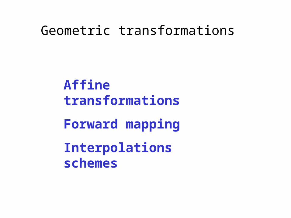
A)    Geometric transformations permit elimination of the geometric distortion that occurs when an image is captured. Geometric distortion may arise because of the lens or because of the irregular movement of the sensor during image capture.

B)     Geometric transformation processing is also essential in situations where there are distortions inherent in the imaging process such as remote sensing from aircraft or spacecraft. On example is an attempt to match remotely sensed images of the same area taken after one year, when the more recent image was probably not taken from precisely the same position. To inspect changes over the year, it is necessary first to execute a geometric transformation, and then subtract one image to other. We might also need to register two or more images of the same scene, obtained from different viewpoints or acquired with different instruments. Image registration matches up the features that are common to two or more images. Registration also finds applications in medical imaging.

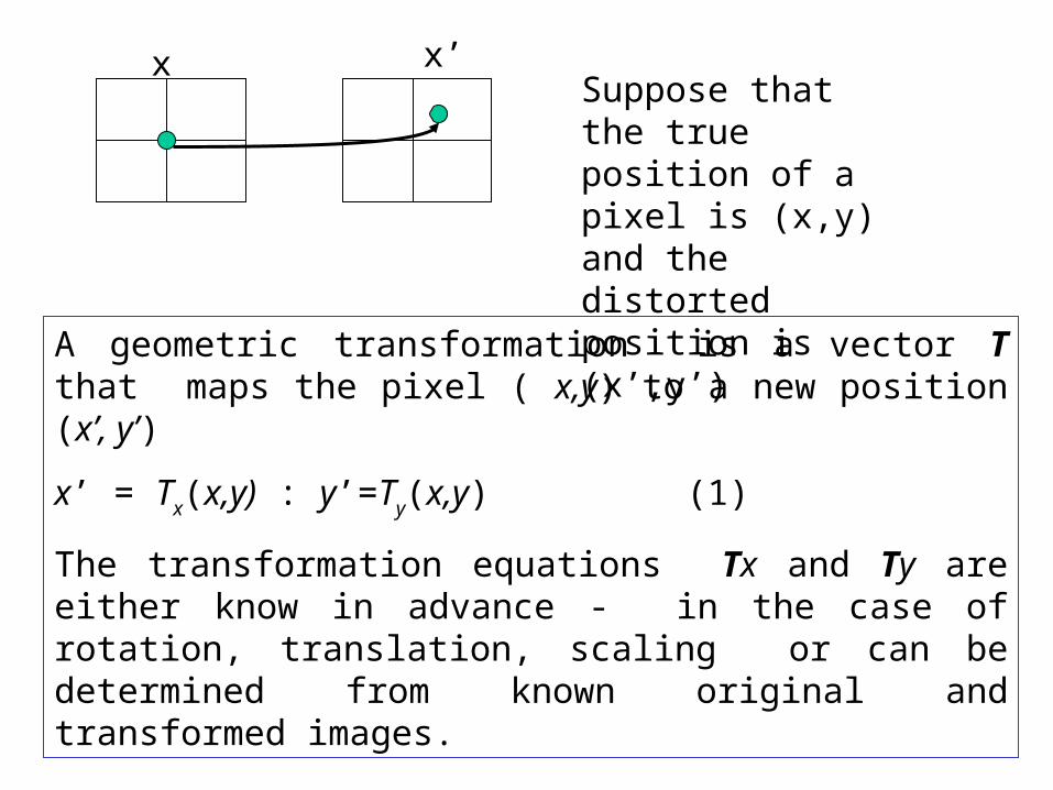
A geometric transformation is a vector T that maps the pixel ( x,y) to a new position (x’, y’)

x’ = Tx(x,y) : y’=Ty(x,y) (1)

The transformation equations Tx and Ty are either know in advance - in the case of rotation, translation, scaling or can be determined from known original and transformed images.

x’xSuppose that the true position of a pixel is (x,y) and the distorted position is (x’,y’)

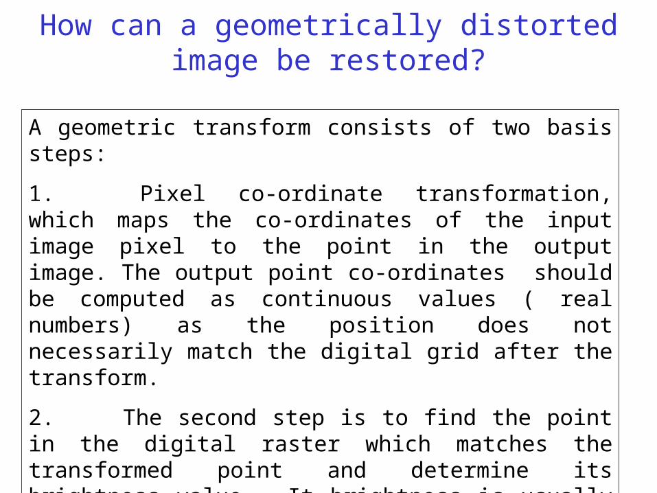
How can a geometrically distorted image be restored?

A geometric transform consists of two basis steps:

1.     Pixel co-ordinate transformation, which maps the co-ordinates of the input image pixel to the point in the output image. The output point co-ordinates should be computed as continuous values ( real numbers) as the position does not necessarily match the digital grid after the transform.

2.     The second step is to find the point in the digital raster which matches the transformed point and determine its brightness value . It brightness is usually computed as an interpolation of the brightness of several points in the neighborhood .

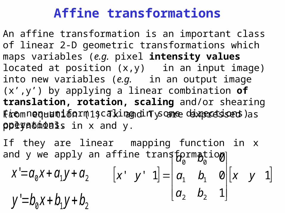
Affine transformations An affine transformation is an important class of linear 2-D geometric transformations which maps variables (e.g. pixel intensity values located at position (x,y) in an input image) into new variables (e.g. in an output image (x’,y’) by applying a linear combination of translation, rotation, scaling and/or shearing (i.e. non-uniform scaling in some directions) operations.

From equation (1) Tx and Ty are expressed as polynomials in x and y.

If they are linear mapping function in x and y we apply an affine transformation

210' ayaxax

210' bybxby

1

1

0

0

1''

22

11

00

yx

ba

ba

ba

yx

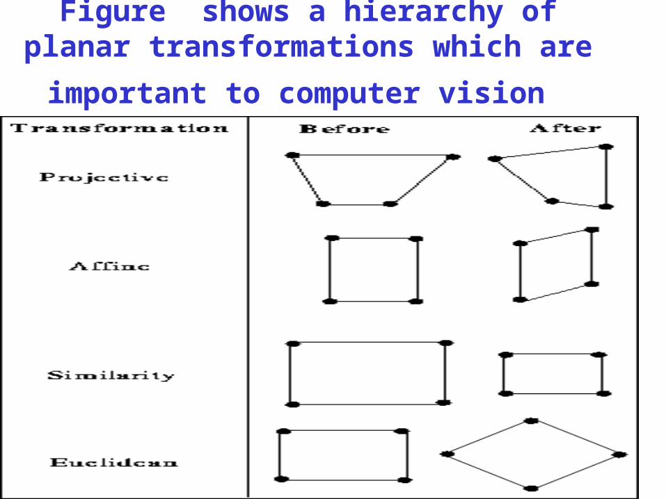
Figure shows a hierarchy of planar transformations which are important to

computer vision

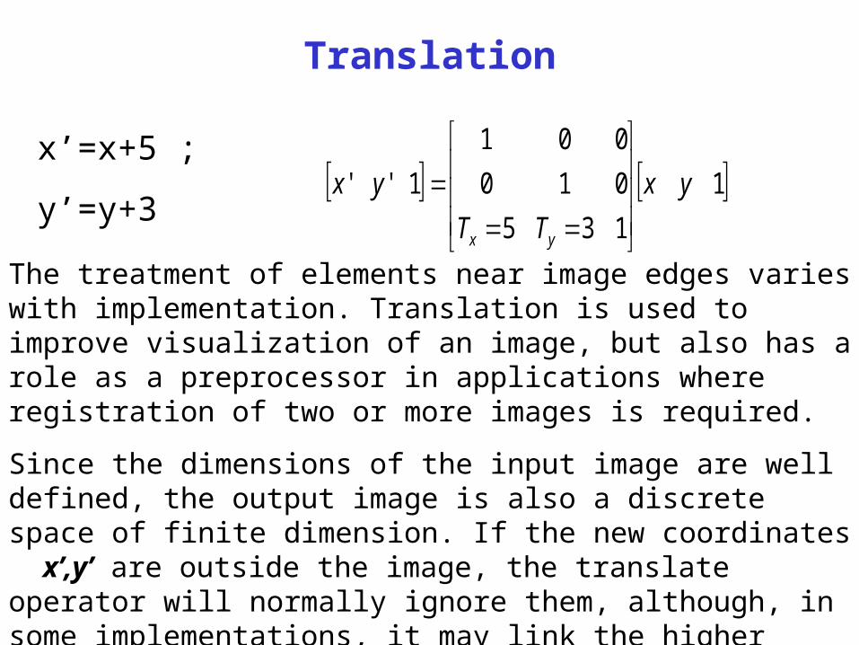
Translation

x’=x+5 ;

y’=y+3 1

135

010

001

1'' yx

TT

yx

yx

The treatment of elements near image edges varies with implementation. Translation is used to improve visualization of an image, but also has a role as a preprocessor in applications where registration of two or more images is required.

Since the dimensions of the input image are well defined, the output image is also a discrete space of finite dimension. If the new coordinates x’,y’ are outside the image, the translate operator will normally ignore them, although, in some implementations, it may link the higher coordinate points with the lower ones so as to wrap the result around back onto the visible space of the image. Most implementations fill the image areas out of which an image has been shifted with black pixels.

Translation Guidelines for Use

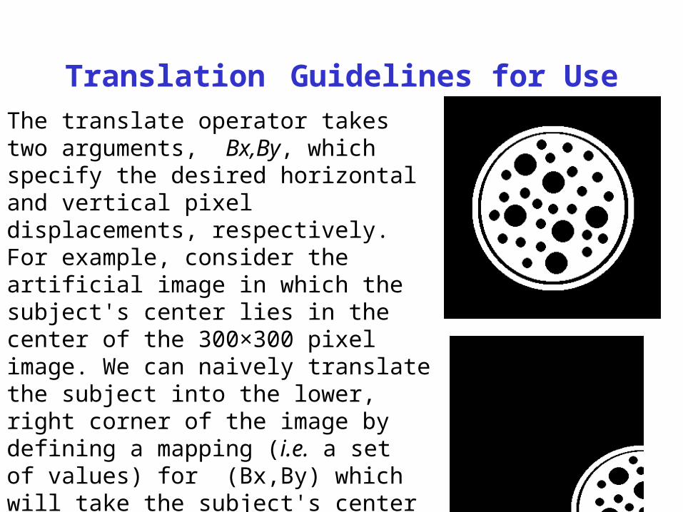
The translate operator takes two arguments, Bx,By, which specify the desired horizontal and vertical pixel displacements, respectively. For example, consider the artificial image in which the subject's center lies in the center of the 300×300 pixel image. We can naively translate the subject into the lower, right corner of the image by defining a mapping (i.e. a set of values) for (Bx,By) which will take the subject's center from its present position at x=150,y=150 to an output position of x=300,y=300 , as shown in the second image

Translation Guidelines for Use

Translation has many applications of the cosmetic sort illustrated above. However, it is also very commonly used as a preprocessor in application domains where registration of two or more images is required. For example, feature detection and spatial filtering algorithms may calculate gradients in such a way as to introduce an offset in the positions of the pixels in the output image with respect to the corresponding pixels from the input image. In the case of the Laplacian of Gaussian spatial sharpening filter, some implementations require that the filtered image be translated by half the width of the Gaussian kernel with which it was convolved in order to bring it into alignment with the original.

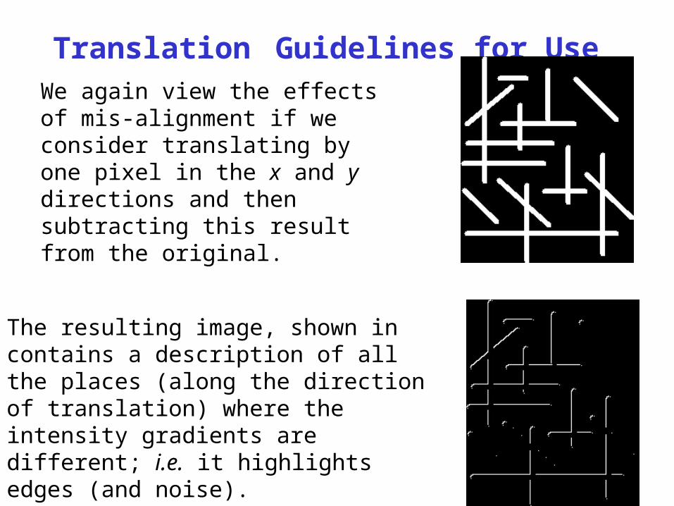
Translation Guidelines for UseWe again view the effects of mis-alignment if we consider translating by one pixel in the x and y directions and then subtracting this result from the original.

The resulting image, shown in contains a description of all the places (along the direction of translation) where the intensity gradients are different; i.e. it highlights edges (and noise).

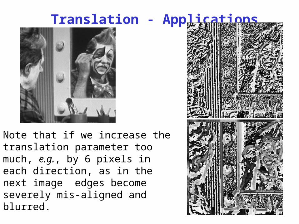
Translation - Applications

Note that if we increase the translation parameter too much, e.g., by 6 pixels in each direction, as in the next image edges become severely mis-aligned and blurred.

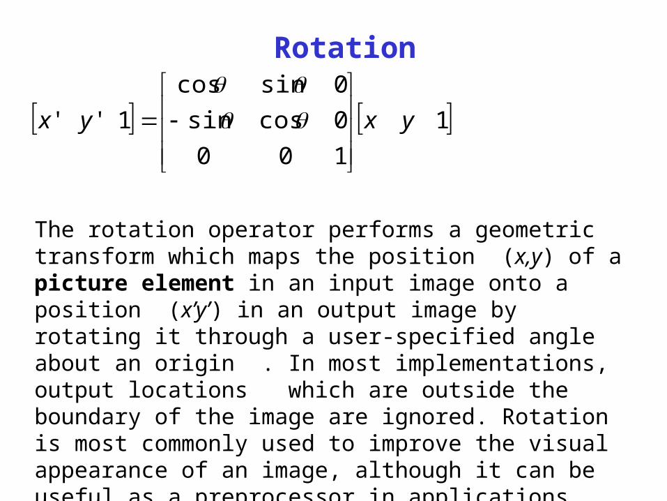
Rotation

1

100

0cossin

0sincos

1'' yxyx

The rotation operator performs a geometric transform which maps the position (x,y) of a picture element in an input image onto a position (x’y’) in an output image by rotating it through a user-specified angle about an origin . In most implementations, output locations which are outside the boundary of the image are ignored. Rotation is most commonly used to improve the visual appearance of an image, although it can be useful as a preprocessor in applications where directional operators are involved.

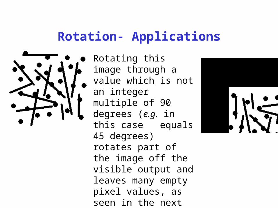
Rotation- Applications

Rotating this image through a value which is not an integer multiple of 90 degrees (e.g. in this case equals 45 degrees) rotates part of the image off the visible output and leaves many empty pixel values, as seen in the next image

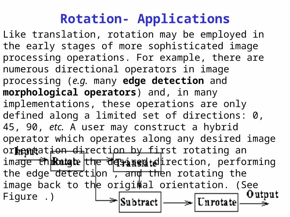
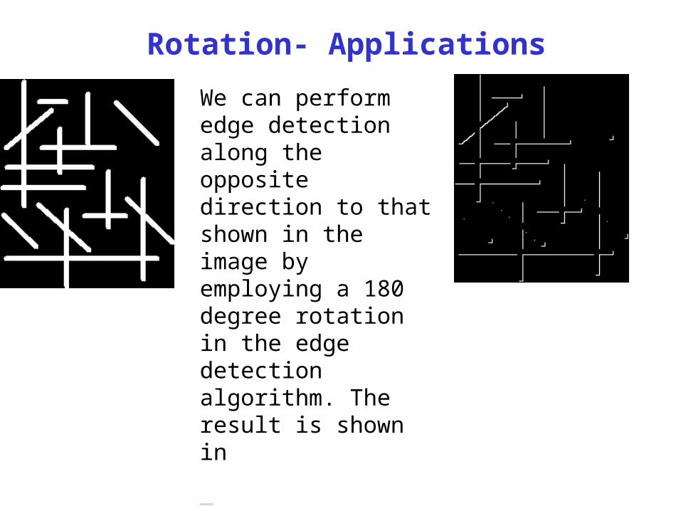
Rotation- ApplicationsLike translation, rotation may be employed in the early stages of more sophisticated image processing operations. For example, there are numerous directional operators in image processing (e.g. many edge detection and morphological operators) and, in many implementations, these operations are only defined along a limited set of directions: 0, 45, 90, etc. A user may construct a hybrid operator which operates along any desired image orientation direction by first rotating an image through the desired direction, performing the edge detection , and then rotating the image back to the original orientation. (See Figure .)

Rotation- Applications

We can perform edge detection along the opposite direction to that shown in the image by employing a 180 degree rotation in the edge detection algorithm. The result is shown in

Geometric Scaling

The scale operator performs a geometric transformation which can be used to shrink or zoom the size of an image (or part of an image). Image reduction, commonly known as subsampling, is performed by replacement (of a group of pixel values by one arbitrarily chosen pixel value from within this group) or by interpolating between pixel values in a local neighborhoods. Image zooming is achieved by pixel replication or by interpolation. Scaling is used to change the visual appearance of an image, to alter the quantity of information stored in a scene representation, or as a low-level preprocessor in multi-stage image processing chain which operates on features of a particular scale.

Scaling compresses or expands an image along the coordinate directions. As different techniques can be used to subsample and zoom

Geometric Scaling

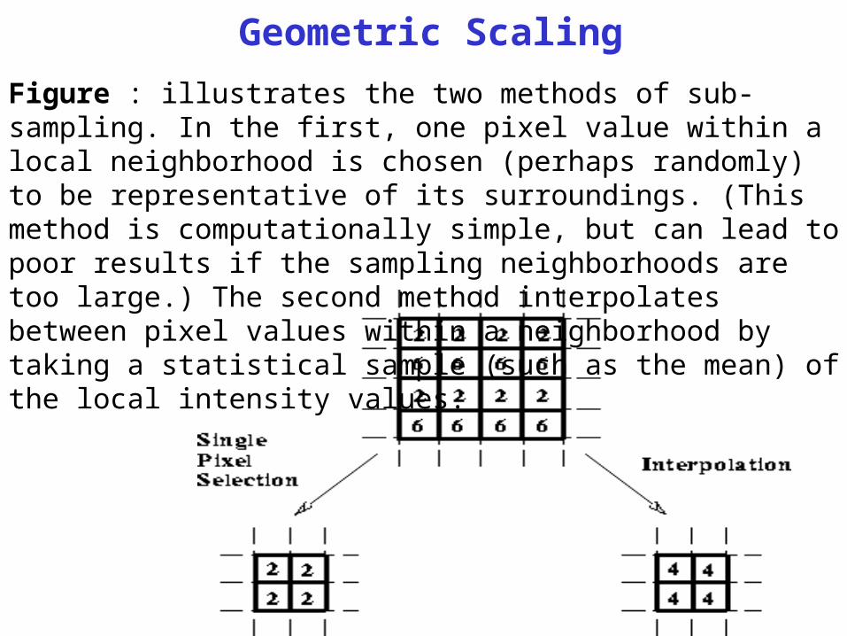
Figure : illustrates the two methods of sub-sampling. In the first, one pixel value within a local neighborhood is chosen (perhaps randomly) to be representative of its surroundings. (This method is computationally simple, but can lead to poor results if the sampling neighborhoods are too large.) The second method interpolates between pixel values within a neighborhood by taking a statistical sample (such as the mean) of the local intensity values.

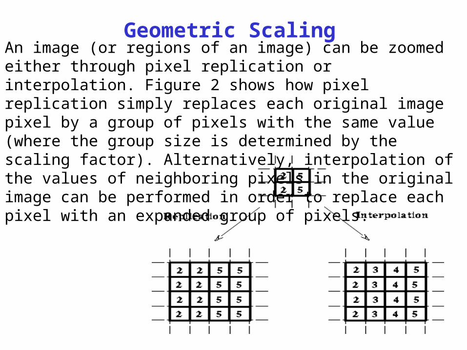
Geometric ScalingAn image (or regions of an image) can be zoomed either through pixel replication or interpolation. Figure 2 shows how pixel replication simply replaces each original image pixel by a group of pixels with the same value (where the group size is determined by the scaling factor). Alternatively, interpolation of the values of neighboring pixels in the original image can be performed in order to replace each pixel with an expanded group of pixels.

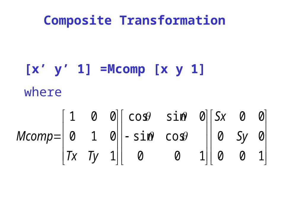
Composite Transformation

100

00

00

100

cossin

0sincos

1

010

001

Sy

Sx

TyTx

Mcomp

[x’ y’ 1] =Mcomp [x y 1]

where

 

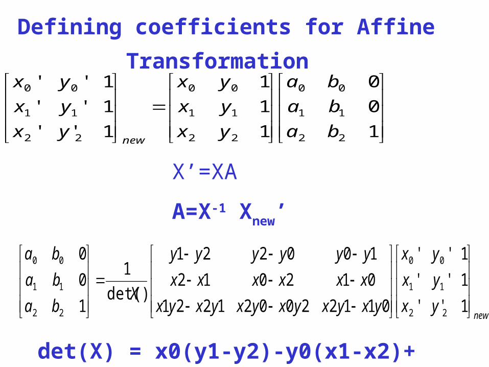
Defining coefficients for Affine Transformation

1

0

0

1

1

1

1''

1''

1''

22

11

00

22

11

00

22

11

00

ba

ba

ba

yx

yx

yx

yx

yx

yx

new

X’=XA

A=X-1 Xnew’

newyx

yx

yx

yxyxyxyxyxyx

xxxxxx

yyyyyy

Xba

ba

ba

1''

1''

1''

011220021221

012012

100221

)det(

1

1

0

0

22

11

00

22

11

00

det(X) = x0(y1-y2)-y0(x1-x2)+(x1y2-x2y1)

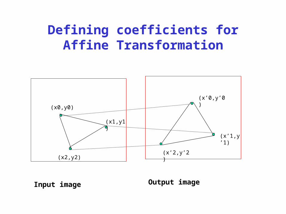
Defining coefficients for Affine Transformation

    

      

      

Input image Output image

(x0,y0)

(x2,y2)

(x1,y1)

(x’1,y’1)

(x’0,y’0)

(x’2,y’2)

 

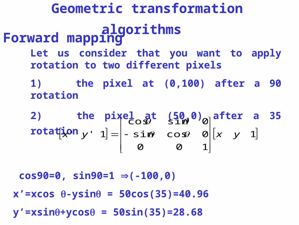
Geometric transformation algorithms Forward mapping

Let us consider that you want to apply rotation to two different pixels

1)     the pixel at (0,100) after a 90 rotation

2)     the pixel at (50,0) after a 35 rotation

1

100

0cossin

0sincos

1'' yxyx

cos90=0, sin90=1 (-100,0)

x’=xcos -ysin = 50cos(35)=40.96

y’=xsin+ycos = 50sin(35)=28.68

Forward mapping

Problems :

1.     Input pixel may map to apposition outside the screen . This problem can be solved by testing coordinates to check that they lie within the bounds of the output image before attempting to copy pixel value.

2.     Input pixel may map to a non-integer position . Simple solution is to find the nearest integers to x’ and y’ and use these integers as a coordinates of the transformed pixel.

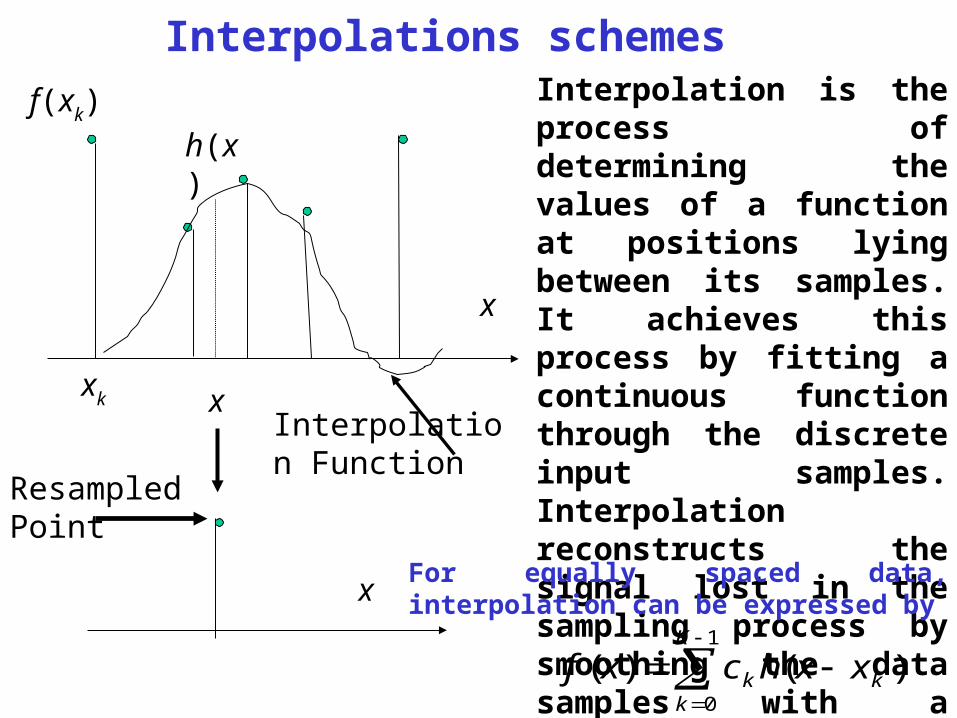
Interpolations schemes Interpolation is the process of determining the values of a function at positions lying between its samples. It achieves this process by fitting a continuous function through the discrete input samples. Interpolation reconstructs the signal lost in the sampling process by smoothing the data samples with a interpolation function. It woks as a low-pass filter.

f(xk)

x

x

x

xk

Interpolation Function

Resampled Point

h(x)

                       

 

For equally spaced data, interpolation can be expressed by

)()(1

0k

K

kk xxhcxf

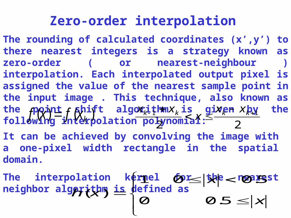
Zero-order interpolation The rounding of calculated coordinates (x’,y’) to there nearest integers is a strategy known as zero-order ( or nearest-neighbour ) interpolation. Each interpolated output pixel is assigned the value of the nearest sample point in the input image . This technique, also known as the point shift algorithm is given by the following interpolation polynomial:

2211

kkkk xx

xxx

)()( kxfxf It can be achieved by convolving the image with a one-pixel width rectangle in the spatial domain.

The interpolation kernel for the nearest neighbor algorithm is defined as

x

xxh

5.00

5.001)(

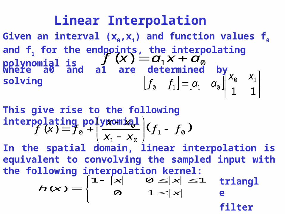
Linear Interpolation Given an interval (x0,x1) and function values f0 and f1 for the

endpoints, the interpolating polynomial is 01)( axaxf

where a0 and a1 are determined by solving

1110

0110

xxaaff

This give rise to the following interpolating polynomial

0101

00)( ff

xx

xxfxf

In the spatial domain, linear interpolation is equivalent to convolving the sampled input with the following interpolation kernel:

x

xxxh

10

101)(

triangle

filter

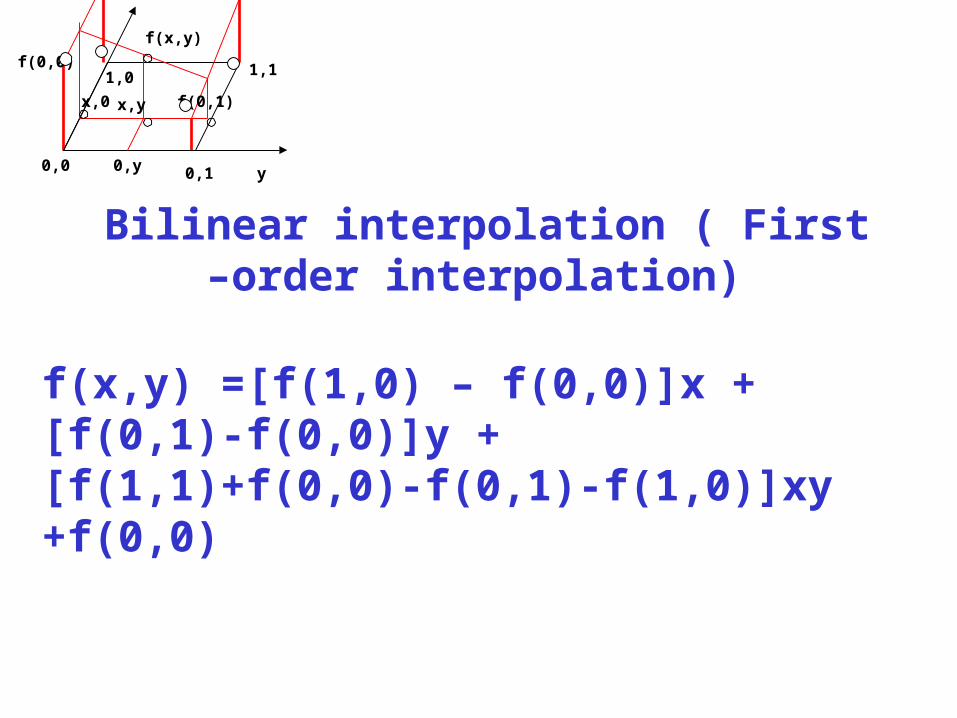
 Bilinear interpolation ( First –order

interpolation)

 

f(0,0)

f(1,1)

x,0 f(0,1)

0,0 0,y 0,1 y

1,1

x,y

f(x,y)

f(1,0)

1,0

 

 

 

 

 

 

 

 

 

 

 

 

 

 

 

f(x,y) =[f(1,0) – f(0,0)]x +[f(0,1)-f(0,0)]y + [f(1,1)+f(0,0)-f(0,1)-f(1,0)]xy +f(0,0)