Embed Size (px)
Citation preview
Getting Started
with
Scienti�c WorkPlaceR
,
Scienti�c WordR
,
and
Scienti�c NotebookR
Version 5


Getting Started
with
Scienti�c WorkPlaceR
,
Scienti�c WordR
,
and
Scienti�c NotebookR
Version 5
Susan BagbyMacKichan Software, Inc.
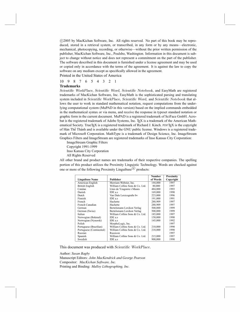
c 2005 by MacKichan Software, Inc. All rights reserved. No part of this book may be repro-duced, stored in a retrieval system, or transcribed, in any form or by any means�electronic,mechanical, photocopying, recording, or otherwise�without the prior written permission of thepublisher, MacKichan Software, Inc., Poulsbo, Washington. Information in this document is sub-ject to change without notice and does not represent a commitment on the part of the publisher.The software described in this document is furnished under a license agreement and may be usedor copied only in accordance with the terms of the agreement. It is against the law to copy thesoftware on any medium except as speci�cally allowed in the agreement.Printed in the United States of America10 9 8 7 6 5 4 3 2 1TrademarksScienti�c WorkPlace, Scienti�c Word, Scienti�c Notebook, and EasyMath are registeredtrademarks of MacKichan Software, Inc. EasyMath is the sophisticated parsing and translatingsystem included in Scienti�c WorkPlace, Scienti�c Word, and Scienti�c Notebook that al-lows the user to work in standard mathematical notation, request computations from the under-lying computational system (MuPAD in this version) based on the implied commands embeddedin the mathematical syntax or via menu, and receive the response in typeset standard notation orgraphic form in the current document. MuPAD is a registered trademark of SciFace GmbH. Acro-bat is the registered trademark of Adobe Systems, Inc. TEX is a trademark of the American Math-ematical Society. TrueTEX is a registered trademark of Richard J. Kinch. PDFTEX is the copyrightof Hàn Thê Thành and is available under the GNU public license. Windows is a registered trade-mark of Microsoft Corporation. MathType is a trademark of Design Science, Inc. ImageStreamGraphics Filters and ImageStream are registered trademarks of Inso Kansas City Corporation:
ImageStream Graphic FiltersCopyright 1991-1999Inso Kansas City CorporationAll Rights Reserved
All other brand and product names are trademarks of their respective companies. The spellingportion of this product utilizes the Proximity Linguistic Technology. Words are checked againstone or more of the following Proximity Linguibase R products:
Number ProximityLinguibase Name Publisher of Words CopyrightAmerican English Merriam-Webster, Inc. 144,000 1997British English William Collins Sons & Co. Ltd. 80,000 1997Catalan Lluis de Yzaguirre i Maura 484,000 1993Danish IDE a.s 169,000 1990Dutch Van Dale Lexicogra�e bv 223,000 1996Finnish IDE a.s 191,000 1991French Hachette 288,909 1997French Canadian Hachette 288,909 1997German Bertelsmann Lexikon Verlag 500,000 1999German (Swiss) Bertelsmann Lexikon Verlag 500,000 1999Italian William Collins Sons & Co. Ltd. 185,000 1997Norwegian (Bokmal) IDE a.s 150,000 1990Norwegian (Nynorsk) IDE a.s 145,000 1992Polish MorphoLogic, Inc. 1997Portuguese (Brazilian) William Collins Sons & Co. Ltd. 210,000 1990Portuguese (Continental) William Collins Sons & Co. Ltd. 218,000 1990Russian Russicon 1997Spanish William Collins Sons & Co. Ltd. 215,000 1997Swedish IDE a.s 900,000 1990
This document was produced with Scienti�c WorkPlace.Author: Susan BagbyManuscript Editors: John MacKendrick and George PearsonCompositor: MacKichan Software, Inc.Printing and Binding: Malloy Lithographing, Inc.
Contents
1 Tools for Scienti�c Creativity 1
Understanding the Product Differences 1
Understanding the New Version 2Compatibility 2Typesetting 2Computation 3
Understanding the Logical Design Approach 3
Using This Booklet 4
Making Sure You Have What You Need 5
Installing and Licensing the Program 5
Exploring the Program 7Start a New Document 7Enter Text and Math 8Change the Screen Appearance of Text 9Compute 9Plot Mathematics 10Print the Document 10Browse the Internet 11Save and Close the Document 11Leave the Program 11
vi Contents
2 Learning the Basics 13
Using the Workplace 13
Opening a Document 14
Entering and Editing Text 15Entering Text 15Editing Text 16
Entering and Editing Mathematics 16Entering Mathematical Characters 17Entering Mathematical Objects 17Entering Mathematics with Fragments 19Using Body Math 20Editing Mathematics 20
Formatting Your Document 20Formatting with Tags 21Formatting the Page 25
Working with Hypertext Links 25Creating Hypertext Links 25Jumping with Hypertext Links 26
Saving Your Document 27Saving Portable LATEX Files 27Exporting Files 28
Previewing and Printing Your Document 28
Working on the Web 29Creating PDF Files 29Exporting Documents as HTML Files 30Using TEX Files on the Web 31Browsing the Internet 31
Managing Your Documents 31
Customizing the Program 33Changing the Appearance of the Toolbars 33Changing the Appearance of the Document Windows 35Changing the Tools and Defaults 36
Contents vii
3 Computing and Plotting 39
Evaluate and Evaluate Numerically 40
Factor 42
Combine 43
Expand 44
Simplify 45
Check Equality 46
Solve Exact and Numeric 47
Work with Polynomials 49
Create 2D and 3D Plots 51
Compute in Place 55
Perform Matrix Operations 56
Solve Differential Equations 57
Compute Statistics 58
Compute with Units of Measure 59
Create Exams and Quizzes 60
4 Typesetting Your Document 61
Understanding the Typesetting Process 62
Typeset Previewing and Typeset Printing 63
Understanding the Appearance of Typeset Documents 64
Creating Typeset Document Elements 65Creating Cross-References 66Creating Notes 67Creating Bibliographies and Citations 67
Obtaining More Information About Typesetting 68
viii Contents
5 Getting the Most from Your Software 69
Using Online Help 70
Obtaining Technical Support 71
Obtaining Additional Information 71
Learning to Use the Program 72
A Toolbars and Buttons 73
B Keyboard Shortcuts 77
Scrolling and Editing 77
Entering Mathematics and Text 79
Index 83
1 Tools for Scienti�c Creativity
Scienti�c WorkPlace, Scienti�c Word, Scienti�c Notebook, and Scienti�c Viewerset the stage for your creativity with their straightforward approach to working withmathematics and text. Together, they combine the ease of entering text and mathematicsin natural notation with the power of symbolic and numeric computation, the �exibilityand beauty of printed or typeset output, and the convenience of direct Internet access.Individually, they offer capabilities and features combined to meet a range of user needs.Version 5 brings new features and enhancements to the MacKichan Software family
of products: typeset PDF output, improved RTF import and export with MathType sup-port, improved HTML and MathML export, and an improved user interface. Scienti�cWorkPlace and Scienti�c Notebook contain the MuPAD computer algebra engine.Explore Version 5 now. Make sure you have what you need to run the software, thencomplete the installation and enter the world of scienti�c creativity.
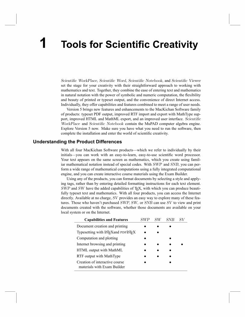
Understanding the Product DifferencesWith all four MacKichan Software products�which we refer to individually by theirinitials�you can work with an easy-to-learn, easy-to-use scienti�c word processor.Your text appears on the same screen as mathematics, which you create using famil-iar mathematical notation instead of special codes. With SWP and SNB, you can per-form a wide range of mathematical computations using a fully integrated computationalengine, and you can create interactive course materials using the Exam Builder.Using any of the products, you can format documents by selecting a style and apply-
ing tags, rather than by entering detailed formatting instructions for each text element.SWP and SW have the added capabilities of TEX, with which you can produce beauti-fully typeset text and mathematics. With all four products, you can access the Internetdirectly. Available at no charge, SV provides an easy way to explore many of these fea-tures. Those who haven't purchased SWP, SW, or SNB can use SV to view and printdocuments created with the software, whether those documents are available on yourlocal system or on the Internet.
Capabilities and Features SWP SW SNB SV
Document creation and printing � � �Typesetting with LATEXand PDFLATEX � �Computation and plotting � �Internet browsing and printing � � � �HTML output with MathML � � �RTF output with MathType � � �Creation of interactive course � �materials with Exam Builder
2 Chapter 1 Tools for Scienti�c Creativity
Understanding the New Version
The program is characterized by a rich interface, beautiful output, natural entry of textand mathematics, and easy creation of complex documents. Version 5 brings additionalcapabilities and features to the workplace.
Compatibility
You can interact with colleagues more easily and distribute your documents in differentformats when you take advantage of new and enhanced export �lters in Version 5.� Export your documents as RTF �les. You can now export your SWP, SW, andSNB documents as Rich Text Format (RTF) �les, so that interactions with colleaguesin non-TEX environments are simpli�ed. The RTF export preserves the formattingyou see in the document window. Any mathematics in your document can be rep-resented with MathType 3 (Equation Editor) or MathType 5 objects. The resultingRTF �le can be viewed in Microsoft Word even if an Equation Editor is not partof the Word installation. If the Microsoft Word installation includes the appropriateEquation Editor, any MathType 3 or MathType 5 mathematical objects in the RTF�le can be edited. The �le can also be displayed in outline mode.
� Read MathType mathematics in RTF �les. In Version 5, you can open and readthe MathType equations in RTF �les when you import the RTF �les in SWP, SW,or SNB. The equations are converted to LATEX.
� Create more accurate HTML �les. When you export your SWP, SW, or SNBdocuments to HTML, the program now places any graphics generated during theprocess in a subdirectory. Version 5 successfully exports �xed-width tables to HTMLand saves the screen format to a Cascading Style Sheet (.css �le). With HTMLexports, you can make your mathematics available on various platforms over theInternet and in applications that can read HTML �les.
� Export mathematics as MathML. When you export HTML �les, you can outputyour mathematics as MathML or graphics. Note that not all HTML browsers supportMathML.
Typesetting
Version 5 of SWP and SW provides new typesetting capabilities and many new docu-ment shells, some intended for international use.� Create typeset PDF �les. Now you can share your work across platforms in PortableDocument Format (PDF) �les by typesetting your SWP and SW documents withPDFLATEX. No extra software is necessary to generate PDF �les. The program auto-matically embeds fonts and graphics in the PDF �le.
� Use PDFTEX to process �les that contain graphics. Until now, using PDFTEX withmost graphics �le formats has been tedious or impossible. Before typesetting yourdocument with PDFLATEX, Version 5 of SWP and SW converts any graphics in thedocument to formats that can be processed by PDFLATEX.
Understanding the Logical Design Approach 3
� Preserve LATEX cross-references in PDF �les. If you add the hyperref package toyour document, any cross-references in your SWP or SW document are convertedto hypertext links when you typeset with PDFLATEX. The package extends hypertextcapabilities with hypertext targets and references. Additionally, PDFLATEX fully linksthe table of contents in the resulting PDF �le and includes in the �le hierarchicalmarkers and thumbnail pictures of all the pages in the document.
� Rotate text in PDF �les. If you create PDF �les from your SWP and SW docu-ments, you can take advantage of the rotating package to rotate parts of text withinthe PDF �le.
� Use expanded typesetting documentation. A new edition of Typesetting Docu-ments in Scienti�c WorkPlace and Scienti�c Word provides more typesetting tips andinformation about more LATEX packages. Learn how to tailor typesetting speci�ca-tions from inside the program to achieve the typeset document appearance you need.
� Examine an expanded gallery of shells. View images of sample documents foreach shell provided with the program in A Gallery of Document Shells for Scienti�cWorkPlace and Scienti�c Word, provided on the program CD as a PDF �le. Use thedocumentation to choose document shells appropriately.
� Choose shells tailored for international documents. Version 5 includes new shellsfor documents created in non-English languages, including German, Japanese, Chi-nese, and Russian. SWP and SW, in combination with TrueTEX, support interna-tional typesetting with the Lambda system.
ComputationComplex computational capability makes SWP and SNB indispensable tools.� Compute with MuPAD. In SWP and SNB, compute right in your document withthe MuPAD computer algebra engine.
� Use enhanced MuPAD capabilities. The new MuPAD kernel is an upgrade fromthe MuPAD 2.0 kernel included in Version 4.0. New features include improved 2Dand 3D plotting, expanded ODE capabilities, an expanded Rewrite submenu, and animproved Simplify operation.
� Compute with MathType mathematics in RTF �les. If you open an RTF �le con-taining MathType equations, the program converts the equations to LATEX. In SWPand SNB, you can compute with the mathematics just like any other mathematics inyour documents.
� Use an improved Exam Builder. The Version 5 Exam Builder is fully functionalwith MuPAD. Printed quizzes can be reloaded without losing their math de�nitions,just like other documents. Exam Builder materials generated with earlier versionsusing either Maple or MuPAD work successfully in Version 5.
Understanding the Logical Design ApproachThe most important feature of the program and the key to our software approach is theseparation of content and appearance. The content of your work results from the creativeprocess of writing�forming ideas and putting them into words. The appearance of your
4 Chapter 1 Tools for Scienti�c Creativity
work results from the mechanical process of formatting�displaying the document onthe screen and on the printed page in the most readable way.Our approach, which is known as logical design, separates the creative process of
writing from the mechanical process of formatting. Logical design frees you to focuson the content instead of its format. It results in increased productivity and a moreconsistent, higher-quality document appearance. Logical design is different from theapproach used by many other word processors. That approach, known as visual design(or sometimes WYSIWYG, for What You See Is What You Get), focuses on making thescreen look as much like the printed page as possible. If you've used only visual systemsbefore now, you may at �rst be surprised by the differences between the two approaches.One major difference is in document formatting. When you use a visual system, you
constantly apply commands that affect the appearance of the content�you select textand then choose a font, a font size, or a typeface, or you apply alignment commandssuch as center, left justify, or right justify. To center a title or an equation, for example,you select it and choose the center alignment.When you use a logical system, you focus on how the content relates logically to
other parts of the document rather than on the appearance of the content. Commands thatde�ne the logical structure of the content replace commands that de�ne its appearance.Thus, instead of applying a centering command to create a centered title, you apply atitle tag to the title information. The properties of the tag you use determine the formatand alignment of the title.In SNB, tag properties are determined by the style, a collection of commands that
de�ne the way the document appears when you display it on the screen and when youproduce it without typesetting. In SWP and SW, tag properties are determined in twoways: by the style and by the document's typesetting speci�cations�a collection ofcommands that de�ne the way the document appears when you produce it with LATEX orPDFLATEX typesetting.Another difference between visual and logical systems is in the display of page di-
visions. On the screen, visual systems divide documents into pages according to theiranticipated appearance in print. To see an entire line, you often have to scroll horizon-tally because the screen dimensions and page dimensions do not match. In a logicalsystem, working with pages is unnecessary, because the division of a document intopages has no connection to the document's logical structure. Thus, on the screen theprogram breaks lines to �t the window. If you resize the window, the program reshapesthe text to �t it. The program displays page divisions when you preview the document.Separating the processes of creating and formatting a document combines the best of
the online and print worlds. You do the work of creating a good document; the programdoes the work of creating a beautiful one.
Using This Booklet
This brief guide to Version 5 of SWP, SW, and SNB explains how to install and registerthe software. It describes how to open, close, save, and manage documents on your localsystem, and how to create documents for and connect to the wider world of informationavailable on the Internet. The booklet explains the basics of using the program to enter,format, edit, preview, and print text and mathematics. It also provides a series of step-by-step examples illustrating how to perform basic mathematical computations and plot
Installing and Licensing the Program 5
mathematical expressions in SWP and SNB. It brie�y discusses using the Exam Builderto create algorithmically generated exams and quizzes. Finally, the booklet explainshow to use the built-in power of LATEX with SWP and SW when you need to produce adocument with a �nely typeset appearance.
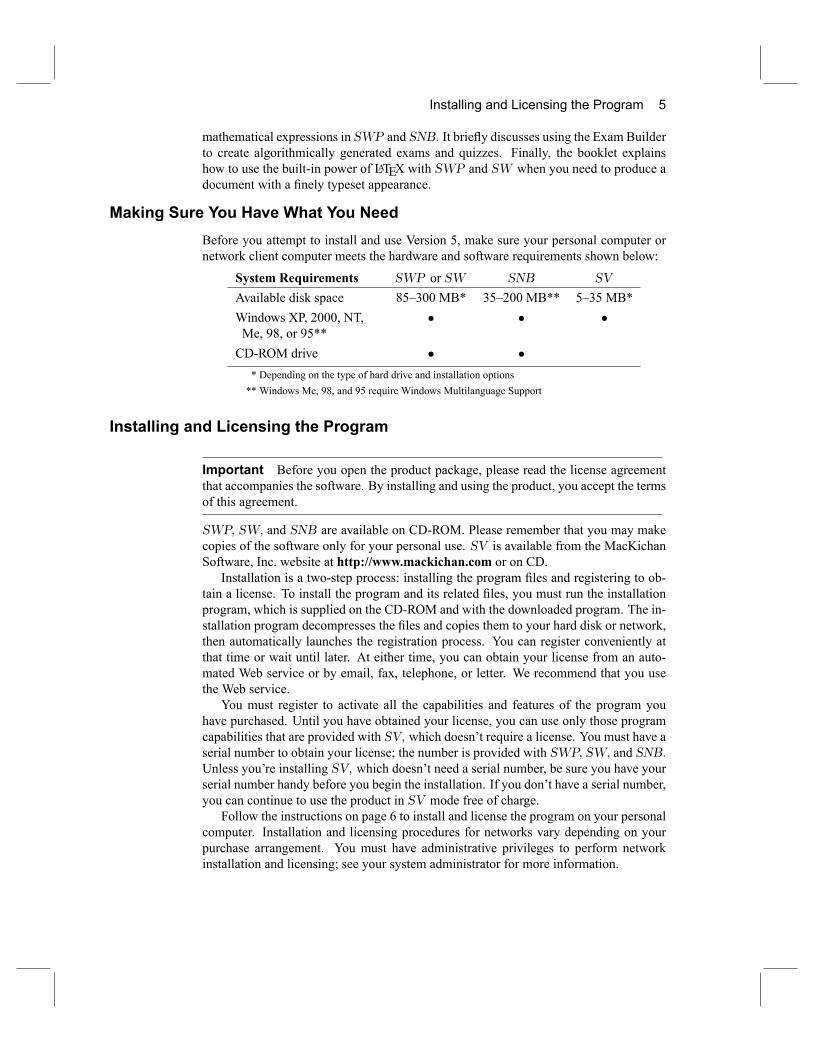
Making Sure You Have What You NeedBefore you attempt to install and use Version 5, make sure your personal computer ornetwork client computer meets the hardware and software requirements shown below:
System Requirements SWP or SW SNB SV
Available disk space 85�300 MB* 35�200 MB** 5�35 MB*Windows XP, 2000, NT, � � �Me, 98, or 95**CD-ROM drive � �* Depending on the type of hard drive and installation options** Windows Me, 98, and 95 require Windows Multilanguage Support
Installing and Licensing the Program
Important Before you open the product package, please read the license agreementthat accompanies the software. By installing and using the product, you accept the termsof this agreement.
SWP, SW, and SNB are available on CD-ROM. Please remember that you may makecopies of the software only for your personal use. SV is available from the MacKichanSoftware, Inc. website at http://www.mackichan.com or on CD.Installation is a two-step process: installing the program �les and registering to ob-
tain a license. To install the program and its related �les, you must run the installationprogram, which is supplied on the CD-ROM and with the downloaded program. The in-stallation program decompresses the �les and copies them to your hard disk or network,then automatically launches the registration process. You can register conveniently atthat time or wait until later. At either time, you can obtain your license from an auto-mated Web service or by email, fax, telephone, or letter. We recommend that you usethe Web service.You must register to activate all the capabilities and features of the program you
have purchased. Until you have obtained your license, you can use only those programcapabilities that are provided with SV, which doesn't require a license. You must have aserial number to obtain your license; the number is provided with SWP, SW, and SNB.Unless you're installing SV, which doesn't need a serial number, be sure you have yourserial number handy before you begin the installation. If you don't have a serial number,you can continue to use the product in SV mode free of charge.Follow the instructions on page 6 to install and license the program on your personal
computer. Installation and licensing procedures for networks vary depending on yourpurchase arrangement. You must have administrative privileges to perform networkinstallation and licensing; see your system administrator for more information.
6 Chapter 1 Tools for Scienti�c Creativity
I To install and license the program on a Windows computer1. Start Windows.
2. If you're installing the program from a CD-ROM, insert the CD-ROM into your CD-ROM drive. Normally, the installation program starts automatically. If it doesn't,
a. From the Windows Start menu, choose Run.b. Choose Browse and select the setup.exe program on the CD.c. Choose OK.
3. If you're installing the program from a downloaded �le,
a. From the Windows Start menu, choose Run.b. Choose Browse and select the .exe program you downloaded.c. Choose OK.
4. Follow the instructions on the screen while the program is installed on your harddisk.
5. When the installation program asks whether you want to register your program,� Choose Yes to register now and open the registration program, then continuethese instructions.or
� Choose No to complete the installation without registering and, when prompted,restart your computer.To register at a later date,i Start the program.ii From the Help menu, choose Register.iii Continue with these instructions, beginning with step 6.
6. If you want to register via the automated Web service,
a. From the Register dialog box, choose By an automated web service and thenchoose Next.
b. Enter the serial number for your program and for any additional dictionaries thatyou have purchased.
c. Enter your email address.Other information is optional.
d. Choose OK.e. Click OK to accept the MacKichan Software license agreement.f. If you aren't already connected to the Internet, dial up your Internet connection.g. Choose Register Now.The program displays a message that your license has been received and saved.
h. Choose Finish.i. Choose OK to close and restart the program.
or
Exploring the Program 7
If you want to register via a different method,
a. From theRegister dialog box, choose the method you want and then chooseNext.b. Follow the instructions on the screen to enter your serial number and other requiredinformation and to accept the license agreement.
c. When you receive your license, follow the accompanying instructions to install it.
7. When the program asks whether you want to restart your computer, choose Yes.
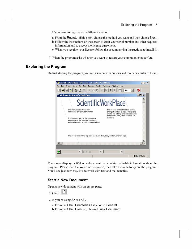
Exploring the ProgramOn �rst starting the program, you see a screen with buttons and toolbars similar to these:
The menus in the Menu barcontain the program commands.
The insertion point in the entry areashows where the program enters textand mathematics or performs operations.
The buttons on the Standard toolbarchange from text to mathematics andinvoke file, editing, and screen displaycommands. Many other toolbars areavailable.
The popup lists in the Tag toolbar provide item, body/section, and text tags.
The screen displays a Welcome document that contains valuable information about theprogram. Please read the Welcome document, then take a minute to try out the program.You'll see just how easy it is to work with text and mathematics.
Start a New DocumentOpen a new document with an empty page.
1. Click .
2. If you're using SNB or SV,
a. From the Shell Directories list, choose General.b. From the Shell Files list, choose Blank Document.
8 Chapter 1 Tools for Scienti�c Creativity
c. Choose OK.d. If you're using SV, choose OK to open an editing window.
or
If you're using SWP or SW,
a. From the Shell Directories list, choose Standard LaTeX.b. From the Shell Files list, choose Blank - Standard LaTeX Article.c. Choose OK.
3. Display several toolbars:
a. From the View menu, choose Toolbars.b. CheckMath Templates and Editing to display the toolbars.c. If you're using SWP or SNB, also check Compute.d. Choose Close.
Enter Text and MathYou can use natural mathematical notation to enter an expression. The program correctlyinterprets your mathematics, which appears in red on your screen by default.1. Type To integrate and press the spacebar.
2. Click to change from text to mathematics.
3. Type x, click , type 2, and press the spacebar.
4. Click to change back to text.
5. Press the spacebar; then type in SWP, enter and press the spacebar.
6. Click .
Note that the program changes to math automatically because it recognizes thatRis
mathematics.
7. Type x, click , type 2, press the spacebar, and then type dx.
On your screen, you should see this:
To integrate x2 in SWP, enterRx2dx
Exploring the Program 9
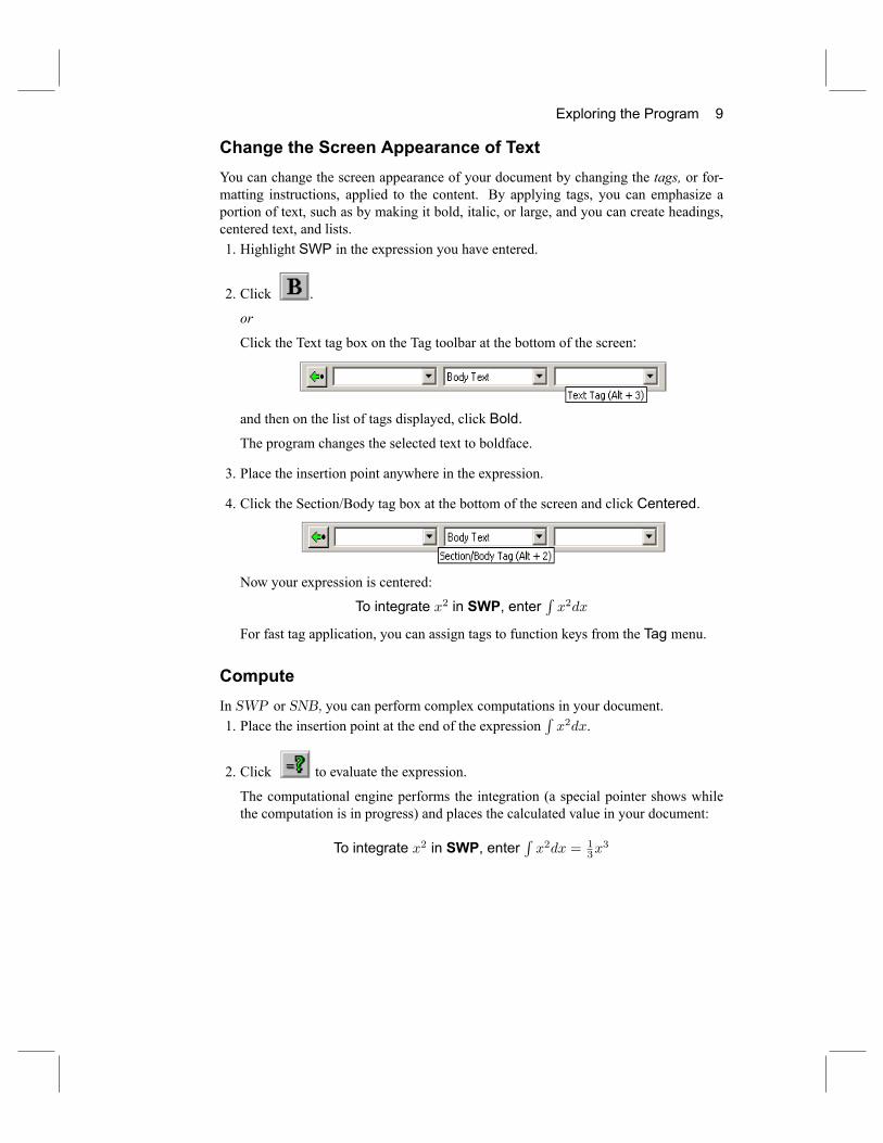
Change the Screen Appearance of TextYou can change the screen appearance of your document by changing the tags, or for-matting instructions, applied to the content. By applying tags, you can emphasize aportion of text, such as by making it bold, italic, or large, and you can create headings,centered text, and lists.1. Highlight SWP in the expression you have entered.
2. Click .
or
Click the Text tag box on the Tag toolbar at the bottom of the screen:
and then on the list of tags displayed, click Bold.
The program changes the selected text to boldface.
3. Place the insertion point anywhere in the expression.
4. Click the Section/Body tag box at the bottom of the screen and click Centered.
Now your expression is centered:
To integrate x2 in SWP, enterRx2dx
For fast tag application, you can assign tags to function keys from the Tag menu.
ComputeIn SWP or SNB, you can perform complex computations in your document.1. Place the insertion point at the end of the expression
Rx2dx.
2. Click to evaluate the expression.
The computational engine performs the integration (a special pointer shows whilethe computation is in progress) and places the calculated value in your document:
To integrate x2 in SWP, enterRx2dx = 1
3x3
10 Chapter 1 Tools for Scienti�c Creativity
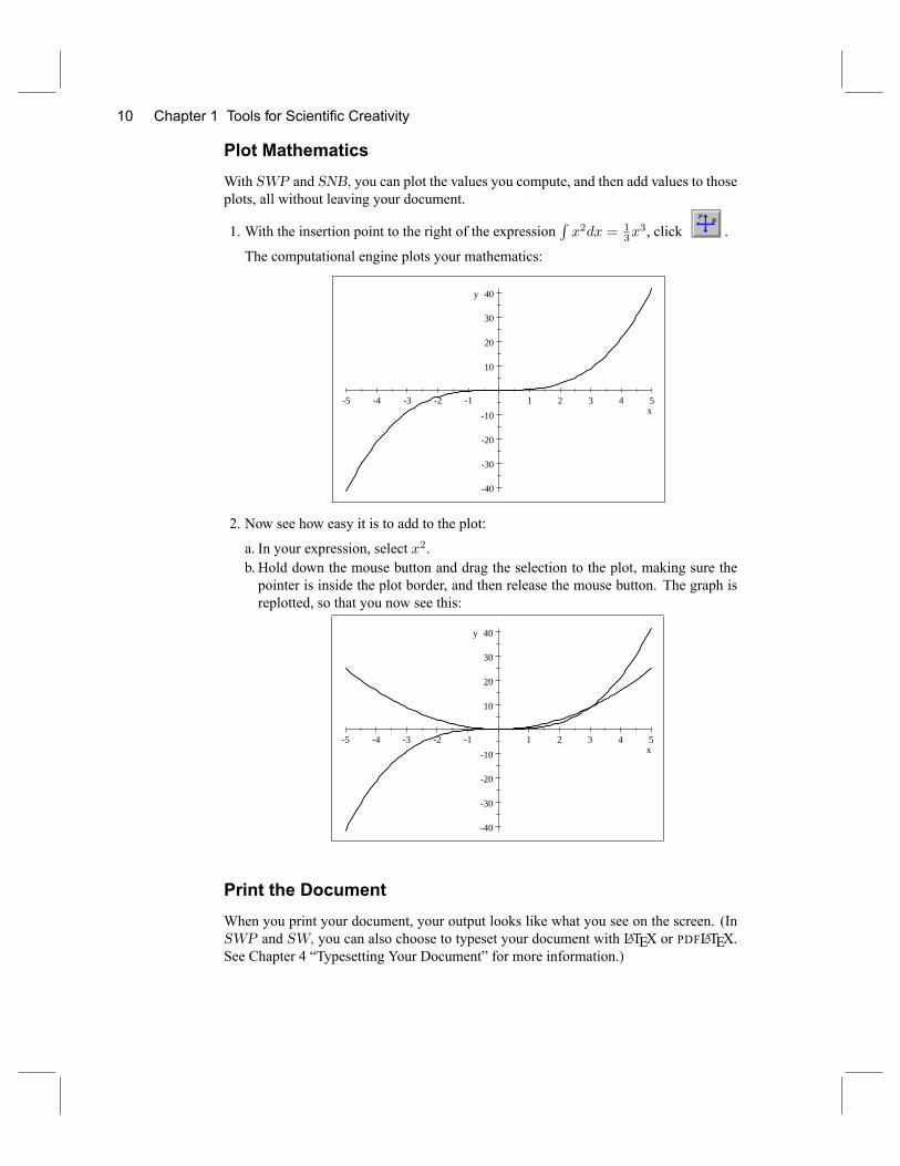
Plot MathematicsWith SWP and SNB, you can plot the values you compute, and then add values to thoseplots, all without leaving your document.
1. With the insertion point to the right of the expressionRx2dx = 1
3x3, click .
The computational engine plots your mathematics:
5 4 3 2 1 1 2 3 4 5
40
30
20
10
10
20
30
40
x
y
2. Now see how easy it is to add to the plot:
a. In your expression, select x2.b. Hold down the mouse button and drag the selection to the plot, making sure thepointer is inside the plot border, and then release the mouse button. The graph isreplotted, so that you now see this:
5 4 3 2 1 1 2 3 4 5
40
30
20
10
10
20
30
40
x
y
Print the DocumentWhen you print your document, your output looks like what you see on the screen. (InSWP and SW, you can also choose to typeset your document with LATEX or PDFLATEX.See Chapter 4 �Typesetting Your Document� for more information.)
Exploring the Program 11
1. Click .
2. In the Print dialog box, select the printer you want to use, and then choose OK.
Browse the InternetIf you have Internet access, you can go directly to any Internet location that has a Uni-form Resource Locator (URL) without ever leaving your document. For example, youcan visit our website, where you can �nd even more information about the program.
1. Click .
2. Enter http://www.mackichan.com and choose Open.
You can specify any URL on the Web. If the location you speci�ed isn't a .tex or.rap document created in SWP, SW, or SNB, the program activates the appropriateprogram on your computer, such as your Web browser or PDF viewer. Your documentremains open. Any SWP, SW, or SNB documents that are available on the Internet areopened as read-only documents.
Save and Close the DocumentSave and close your document, unless you are using SV.
1. Click .
2. Type a name for the document and choose OK.
3. From the File menu, choose Close.
Leave the ProgramYou can leave the program several ways. If you haven't saved your SWP, SW, or SNBdocument, the program prompts you to save your work.� From the File menu, choose Exit.or
� Press ALT+F4 (that is, hold down the ALT key and press F4).or
� At the top right corner of the program window, click the Close button .or
� At the top left corner of the program window, double-click the program icon, or clickthe icon once and then choose Close.

2 Learning the Basics
SWP, SW, and SNB are intuitive. Whether you're writing text or mathematics, you'll�nd that using the program is easy.
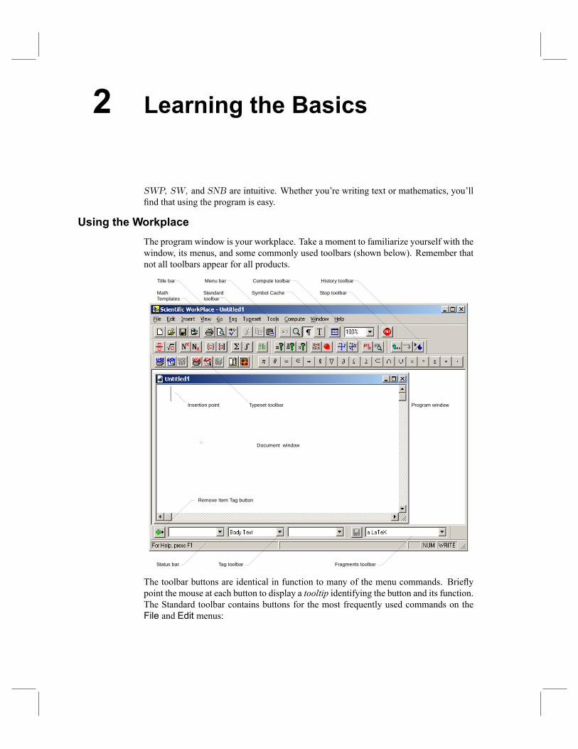
Using the WorkplaceThe program window is your workplace. Take a moment to familiarize yourself with thewindow, its menus, and some commonly used toolbars (shown below). Remember thatnot all toolbars appear for all products.
Status bar Tag toolbar Fragments toolbar
Remove Item Tag button
Insertion point Typeset toolbar Program window
Title bar Menu bar Compute toolbar History toolbar
Math Standard Symbol Cache Stop toolbarTemplates toolbar
Document window
The toolbar buttons are identical in function to many of the menu commands. Brie�ypoint the mouse at each button to display a tooltip identifying the button and its function.The Standard toolbar contains buttons for the most frequently used commands on theFile and Edit menus:
14 Chapter 2 Learning the Basics
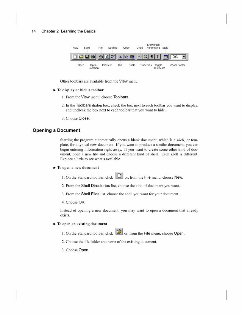
Show/HideNew Save Print Spelling Copy Undo Nonprinting Table
Open Open Preview Cut Paste Properties Toggle Zoom FactorLocation Text/Math
Other toolbars are available from the View menu.
I To display or hide a toolbar1. From the View menu, choose Toolbars.
2. In the Toolbars dialog box, check the box next to each toolbar you want to display,and uncheck the box next to each toolbar that you want to hide.
3. Choose Close.
Opening a Document
Starting the program automatically opens a blank document, which is a shell, or tem-plate, for a typical new document. If you want to produce a similar document, you canbegin entering information right away. If you want to create some other kind of doc-ument, open a new �le and choose a different kind of shell. Each shell is different.Explore a little to see what's available.
I To open a new document
1. On the Standard toolbar, click or, from the File menu, choose New.
2. From the Shell Directories list, choose the kind of document you want.
3. From the Shell Files list, choose the shell you want for your document.
4. Choose OK.
Instead of opening a new document, you may want to open a document that alreadyexists.
I To open an existing document
1. On the Standard toolbar, click or, from the File menu, choose Open.
2. Choose the �le folder and name of the existing document.
3. Choose Open.
Entering and Editing Text 15
Entering and Editing TextEntering information is straightforward, whether you prefer the keyboard or the mouse.You use standard editing tools to revise your document.
Entering TextUnless you tell it otherwise, the program assumes that everything you type is text. When
you're entering text, the Math/Text toggle on the Standard toolbar appears as .
I To enter text, just start typing.Although most keyboards don't contain special text characters, you can enter many
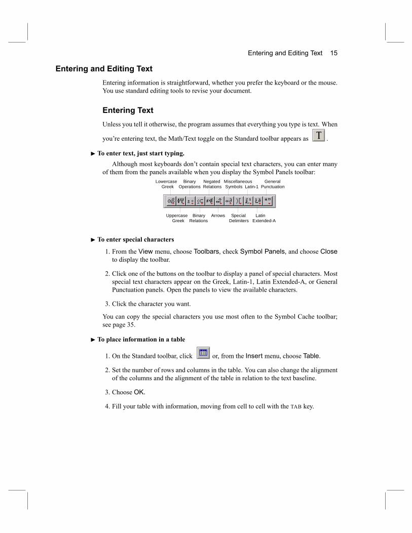
of them from the panels available when you display the Symbol Panels toolbar:Lowercase Binary Negated Miscellaneous General
Greek Operations Relations Symbols Latin1 Punctuation
Uppercase Binary Arrows Special LatinGreek Relations Delimiters ExtendedA
I To enter special characters1. From the View menu, choose Toolbars, check Symbol Panels, and choose Closeto display the toolbar.
2. Click one of the buttons on the toolbar to display a panel of special characters. Mostspecial text characters appear on the Greek, Latin-1, Latin Extended-A, or GeneralPunctuation panels. Open the panels to view the available characters.
3. Click the character you want.
You can copy the special characters you use most often to the Symbol Cache toolbar;see page 35.
I To place information in a table
1. On the Standard toolbar, click or, from the Insert menu, choose Table.
2. Set the number of rows and columns in the table. You can also change the alignmentof the columns and the alignment of the table in relation to the text baseline.
3. Choose OK.
4. Fill your table with information, moving from cell to cell with the TAB key.
16 Chapter 2 Learning the Basics
Editing TextOnce you've entered your text, you may need to edit it. You can use standard clipboardand drag-and-drop operations to cut, copy, paste, and delete selections. If you changeyour mind, you can undo the most recent change or deletion. To help revise your content,you can also use the spell check feature available from the Tools menu or the Standardtoolbar, and the �nd and replace feature, available from the Edit menu or the Editingtoolbar.
I To undo your most recent change or deletion
� On the Standard toolbar, click or, from the Edit menu, choose Undo.Another way to edit text is by changing the properties of individual characters. For
example, you might add an accent to a character so that a becomes ä.
I To edit the properties of a character1. Select the character or place the insertion point to its right.
2. Open the Character Properties dialog box:
� On the Standard toolbar, click .or
� From the Edit menu, choose Properties.or
� Press CTRL+F5 (hold down the CTRL key and press F5).or
� Click the right mouse button or press the Application key to open theContext menu and then choose Properties.
3. Make the changes you want, and then choose OK.
Entering and Editing MathematicsBecause the program assumes you're entering text, you must tell it when you want toenter mathematics. Then, you can enter mathematics easily using the toolbar buttons,Insert menu commands, or keyboard shortcuts.
I To start mathematics
� On the Standard toolbar, click or, from the Insert menu, chooseMath.
When mathematics is active, the Math/Text toggle appears as .
I To return to text
� On the Standard toolbar, click or, from the Insert menu, choose Text.
When text is active, the Math/Text toggle appears as .
Entering and Editing Mathematics 17
Entering Mathematical CharactersMathematical characters and symbols are available from the customizable Symbol Cachetoolbar and the symbol panels. We suggest you open the symbol panels one by one toexplore all the available characters. Choosing a mathematical character automaticallystarts mathematics, even if you have not toggled to mathematics.
I To enter a mathematical character1. From the View menu, display the Symbol Cache and Symbol Panels toolbars.
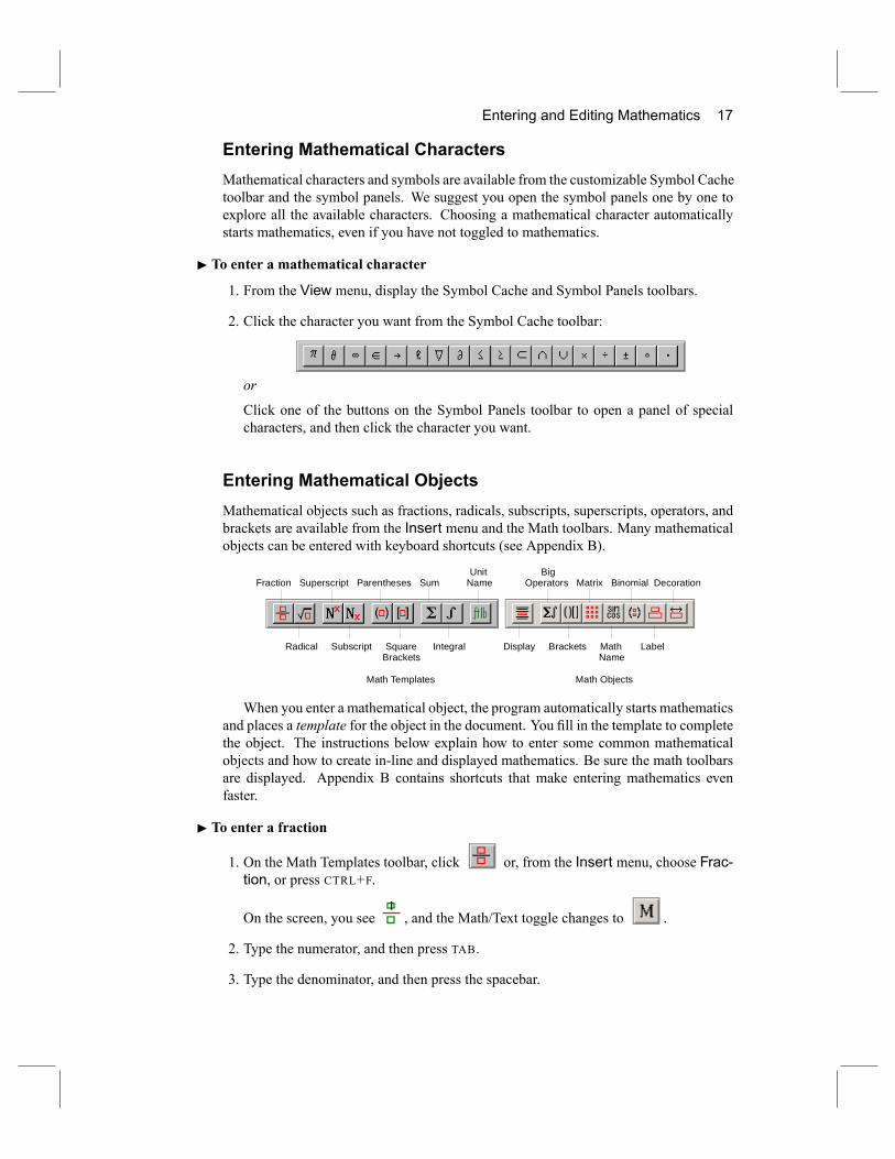
2. Click the character you want from the Symbol Cache toolbar:
or
Click one of the buttons on the Symbol Panels toolbar to open a panel of specialcharacters, and then click the character you want.
Entering Mathematical ObjectsMathematical objects such as fractions, radicals, subscripts, superscripts, operators, andbrackets are available from the Insert menu and the Math toolbars. Many mathematicalobjects can be entered with keyboard shortcuts (see Appendix B).
Unit BigFraction Superscript Parentheses Sum Name Operators Matrix Binomial Decoration
Radical Subscript Square Integral Display Brackets Math LabelBrackets Name
Math Templates Math Objects
When you enter a mathematical object, the program automatically starts mathematicsand places a template for the object in the document. You �ll in the template to completethe object. The instructions below explain how to enter some common mathematicalobjects and how to create in-line and displayed mathematics. Be sure the math toolbarsare displayed. Appendix B contains shortcuts that make entering mathematics evenfaster.
I To enter a fraction
1. On the Math Templates toolbar, click or, from the Insert menu, choose Frac-tion, or press CTRL+F.
On the screen, you see , and the Math/Text toggle changes to .
2. Type the numerator, and then press TAB.
3. Type the denominator, and then press the spacebar.
18 Chapter 2 Learning the Basics
I To enter a superscript or subscript
1. Click or, from the Insert menu, chooseMath to start mathematics.
2. Type a variable.
3. On the Math Templates toolbar, click or press CTRL+UP ARROW to enter asuperscript.
or
On the Math Templates toolbar, click or press CTRL+DOWN ARROW to entera subscript.
4. Type the superscript or subscript, and then press the spacebar.
I To enter an expression in parentheses
1. On the Math Templates toolbar, click .
2. Type the expression. Notice that the parentheses are elastic�they expand horizon-tally and vertically as far as necessary to enclose the expression you enter.
3. Press the spacebar.
I To enter a matrix
1. On the Math Objects toolbar, click or, from the Insert menu, chooseMatrix.
2. Set the number of rows and columns, the alignment, and the baseline of the matrix.
3. Choose the delimiters for the matrix, if desired.
4. Choose OK.
5. Fill your matrix with mathematics, moving from cell to cell with the TAB key.
6. Press the spacebar to leave the matrix.
I To enter an operator
1. On the Math Objects toolbar, click or, from the Insert menu, choose Opera-tor.
2. Double-click the operator you want.
3. On the Math Templates toolbar, click and then type the lower limit for theoperator.
Entering and Editing Mathematics 19
4. Press TAB, and then type the upper limit.
5. Press the spacebar, and then type the variable.
6. If the variable carries a subscript, click , type the subscript, and then press thespacebar.
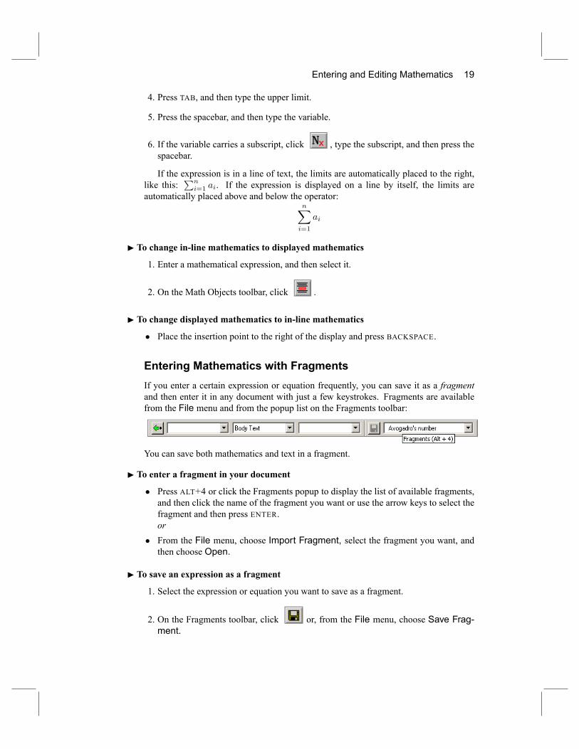
If the expression is in a line of text, the limits are automatically placed to the right,like this:
Pni=1 ai. If the expression is displayed on a line by itself, the limits are
automatically placed above and below the operator:nXi=1
ai
I To change in-line mathematics to displayed mathematics1. Enter a mathematical expression, and then select it.
2. On the Math Objects toolbar, click .
I To change displayed mathematics to in-line mathematics� Place the insertion point to the right of the display and press BACKSPACE.
Entering Mathematics with FragmentsIf you enter a certain expression or equation frequently, you can save it as a fragmentand then enter it in any document with just a few keystrokes. Fragments are availablefrom the File menu and from the popup list on the Fragments toolbar:
You can save both mathematics and text in a fragment.
I To enter a fragment in your document� Press ALT+4 or click the Fragments popup to display the list of available fragments,and then click the name of the fragment you want or use the arrow keys to select thefragment and then press ENTER.or
� From the File menu, choose Import Fragment, select the fragment you want, andthen choose Open.
I To save an expression as a fragment1. Select the expression or equation you want to save as a fragment.
2. On the Fragments toolbar, click or, from the File menu, choose Save Frag-ment.
20 Chapter 2 Learning the Basics
3. Type a �le name to be used to recall the fragment. Avoid using the name of a TEXcommand for the fragment. If you leave the directory unchanged, your fragment willappear in the top part of the list of available fragments. You can create subdirectoriesfor fragments.
4. Choose Save.
Using Body Math
You can enter a series of mathematical expressions quickly if you enter them in a BodyMath paragraph. The Body Math tag is available from the Section/Body Tag popuplist. Each time you press ENTER in a Body Math paragraph, the program automaticallyswitches to mathematics. This makes it easy to use your document as a mathematicsscratchpad. See Formatting with Tags on page 21.
Editing Mathematics
When you need to edit your mathematics, you can use standard clipboard and drag-and-drop operations to cut, copy, paste, and delete. You can also edit the properties ofmathematical characters, symbols, and objects.When you edit the properties of a mathematical character or symbol, the program
opens the Character Properties dialog box. When you edit the properties of a math-ematical object, the program opens a context-sensitive dialog box; that is, a dialog boxthat corresponds to the mathematical object you've selected. If you haven't selected anobject, the program opens the dialog box appropriate for the object to the left of theinsertion point.
I To edit the properties of a mathematical object1. Select the object or place the insertion point to its right.
2. Open a context-sensitive Properties dialog box:
� Click .or
� From the Edit or Context menu, choose Properties.or
� Press CTRL+F5.
3. Make the changes you want, and then choose OK.
Formatting Your Document
In SWP, SW, and SNB, you can produce your document without typesetting it. InSWP and SW, you can also typeset your document. The appearance of your documentdepends on which method you use.
Formatting Your Document 21
� If you display your document in the document window or produce it without type-setting, the program formats the document using the document style (.cst) �le, thepage setup speci�cations, and the Document Info print options.
� If you typeset your document, the program formats the document using the typeset-ting speci�cations, including the document class options, any LATEX package options,and any TEX commands that have been added to the document. Chapter 4 �Typeset-ting Your Document� has more information.
Formatting with TagsBoth the document style and the typesetting speci�cations de�ne tags�collections offormatting and behavior properties that determine the appearance of your document. Theproperties de�ne the type face, font size, font style, paragraph indention, justi�cation,and many other aspects of document appearance. When you apply a tag to information inyour document, the program applies the formatting and behavior properties associatedwith the tag to that information. Using tags, you can create a consistent appearancethroughout your document without having to format each element individually.Tag properties are de�ned in the style �le for the shell you used to create your docu-
ment. In SWP and SW, tag properties are also de�ned in the typesetting speci�cationsfor the shell. In SWP and SW, the way you produce your document determines whichset of properties the program uses.The program has section/body tags, item tags, and text tags. Everything you enter
in your document carries one or more tags. The program automatically applies theBody Text tag to all text that you enter. By changing the Body Text tag to a differentsection/body tag, you can create a heading or a centered paragraph, and by adding anitem tag, you can create a list.In addition to applying tags from the popup lists at the bottom of the program win-
dow, as described in these instructions, you can apply tags with the function keys andwith the Apply command on the Tag menu.
I To enter a heading1. Press ALT+2 or click the Section/Body Tag popup list:
2. From the tag list that pops up, click the heading level you want.
3. Type the text of the heading and then press ENTER.
I To center text1. Press ALT+2 or click the Section/Body Tag popup list.
2. From the tag list that pops up, click the centering tag you want.
3. Type the text to be centered and then press ENTER.
4. Click the Section/Body Tag popup list again and click the Body Text tag.
22 Chapter 2 Learning the Basics
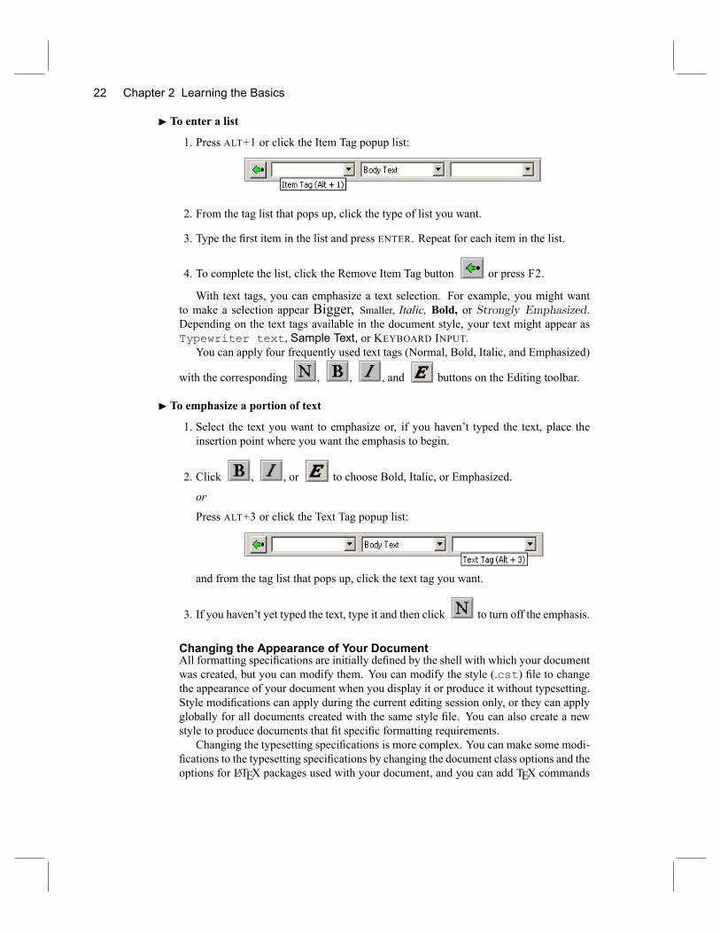
I To enter a list1. Press ALT+1 or click the Item Tag popup list:
2. From the tag list that pops up, click the type of list you want.
3. Type the �rst item in the list and press ENTER. Repeat for each item in the list.
4. To complete the list, click the Remove Item Tag button or press F2.
With text tags, you can emphasize a text selection. For example, you might wantto make a selection appear Bigger, Smaller, Italic, Bold, or Strongly Emphasized.Depending on the text tags available in the document style, your text might appear asTypewriter text, Sample Text, or KEYBOARD INPUT.You can apply four frequently used text tags (Normal, Bold, Italic, and Emphasized)
with the corresponding , , , and buttons on the Editing toolbar.
I To emphasize a portion of text1. Select the text you want to emphasize or, if you haven't typed the text, place theinsertion point where you want the emphasis to begin.
2. Click , , or to choose Bold, Italic, or Emphasized.
or
Press ALT+3 or click the Text Tag popup list:
and from the tag list that pops up, click the text tag you want.
3. If you haven't yet typed the text, type it and then click to turn off the emphasis.
Changing the Appearance of Your DocumentAll formatting speci�cations are initially de�ned by the shell with which your documentwas created, but you can modify them. You can modify the style (.cst) �le to changethe appearance of your document when you display it or produce it without typesetting.Style modi�cations can apply during the current editing session only, or they can applyglobally for all documents created with the same style �le. You can also create a newstyle to produce documents that �t speci�c formatting requirements.Changing the typesetting speci�cations is more complex. You can make some modi-
�cations to the typesetting speci�cations by changing the document class options and theoptions for LATEX packages used with your document, and you can add TEX commands
Formatting Your Document 23
to the preamble, front matter, and body of the document. However, extensive modi�-cation of the typesetting speci�cations isn't advisable and requires a knowledge of TEXand LATEX. Please see Chapter 4 �Typesetting Your Document� for more informationabout changing the typesetting speci�cations.
Modifying the Tag Properties De�ned in the StyleYou can change the way tagged text appears in the document window and when youproduce it without typesetting if you modify the tag properties de�ned in the style (.cst)�le for the document shell. Tag properties have some subtle characteristics.� Basic properties. Tag properties de�ne the appearance of tagged text in terms of thetag type font; the spacing, background color, and indention of tagged paragraphs;the color and size of mathematics and mathematical objects that occur in taggedtext; and the behavior of the tag. Tag properties also de�ne the appearance of specialobjects (such as citations, lead-in objects, tables, and mathematical displays) whenthey occur within tagged text.
� Nested properties. Tags can be nested and so can their properties. The style deter-mines the properties to use beginning with the innermost tag.
� Inherited properties. Rather than specifying a value for a tag property, the style canspecify that the property inherit its values from the surrounding text.
� Unspeci�ed properties. If the style doesn't de�ne a speci�c or inherited value fora particular tag property, the style uses the corresponding property value for thesurrounding tag.
� Default properties. When no other properties apply in a given context, the styleuses default properties.
Examples illustrating these characteristics appear in the online Help.
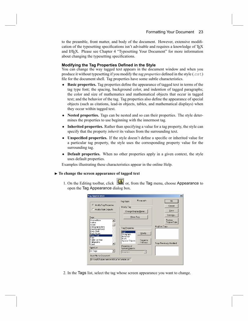
I To change the screen appearance of tagged text
1. On the Editing toolbar, click or, from the Tag menu, choose Appearance toopen the Tag Appearance dialog box.
2. In the Tags list, select the tag whose screen appearance you want to change.
24 Chapter 2 Learning the Basics
3. In the Tag Properties area, select the property and, if necessary, the special objectthat you want to change, and then choose Modify.
In addition to many others, these properties are available for most tags:
Choose To modify the appearance ofFont Type face, size, style, and colorParagraph Justi�cation, indention, line spacing, background colorBehavior Tag for the following paragraph; appearance of the
tag name in popup listsMath Screen color, size, and placement of mathematical objectsSpecial Objects Citations, lead-in objects, tables, matrices, displays,
graphic and plot captions, formulas, input buttons,hypertext links, hypertext markers, and cross-references
4. Make the changes you want in the property dialog box and then choose OK.
5. Repeat steps 2-4 for all tags whose style properties you want to change.
6. If you decide you don't want the changes for a particular tag property,
a. Select the tag.b. Select the property in the Tag Properties area.c. Choose Revert to Previous.
7. If you decide you don't want any of the tag property changes, choose Restore Orig-inal Style to return to the settings saved in the style �le.
8. Save the changes:� Choose Save to save the changes to the current style �le, which is listed in thebox labeled Style File for Document. This will alter the screen appearance ofall documents created with the style.or
� Choose Save As to save the settings in a new style �le. Enter a name for the new�le and choose Save.
9. Choose OK.
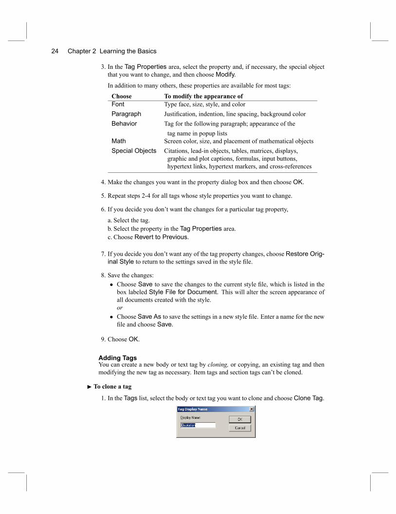
Adding TagsYou can create a new body or text tag by cloning, or copying, an existing tag and thenmodifying the new tag as necessary. Item tags and section tags can't be cloned.
I To clone a tag1. In the Tags list, select the body or text tag you want to clone and choose Clone Tag.
Working with Hypertext Links 25
2. Enter a name for the new tag and choose OK.
The program displays the name in the Tags list and in the corresponding tag popuplist in the program window.
3. In the Tags list, select the new tag.
4. Select and modify the tag properties as necessary, and then choose OK.
5. Save the changes in the same style (.cst) �le or as a new style.
Formatting the PageIf you produce your document without typesetting it, the margins, headers, footers, andpage numbers are set initially by the page setup speci�cations for the document shell.Margins, headers, footers, and page numbers don't appear in the document window, butyou can see them when you preview. You can change them to suit your needs.
I To modify the page setup speci�cations1. From the File menu, choose Page Setup.
2. Choose the tab you need:
Choose ToMargins Set the left, right, top, and bottom page marginsHeaders/Footers Specify headers, footers, and page numberingCounters Specify the page numbering style
3. Make the necessary modi�cations.
4. Choose OK.
Remember that if you typeset your document in SWP or SW, the program ignoresthe page setup speci�cations, and sets the margins, headers, footers, and page numbersaccording to the typesetting speci�cations.
Working with Hypertext LinksYou can use hypertext links, or jumps, to link your document to information in anotherlocation. You can access information located elsewhere in the same document, in otherdocuments on the current system or network, or, if you have Internet access, on the Web.See Browsing the Internet on page 31 for more information.
Creating Hypertext LinksHypertext links have two parts: the link and the target. The link creates a pointer to thetarget and de�nes the appearance of the pointer in your document. (Read more abouthypertext links and typesetting in Creating Documents with Scienti�c WorkPlace andScienti�c Word and in the online Help.)
26 Chapter 2 Learning the Basics
The target of a hypertext jump can be any object to which you've assigned an iden-tifying key or marker�such as a �gure, a section, or equation�or any �le, including�les on the Internet. The address of the target differs depending on the target itself andfollows the model used in standard Web browsers.
I To create a hypertext link1. Place the insertion point where you want the link to appear.
2. On the Field toolbar, click or, from the Insert menu, choose Hypertext Link.
3. In the Hypertext Link dialog box, enter the screen text for the link. The screen textcan contain a graphic.
See the online Help for information about printing documents containing hypertextlinks.
4. In the Target box, enter the address of the target:� If the target is outside the current document, enter the document address in theURL box, and the marker, if any, in the Marker box.
� If the target is inside the current document, enter the marker in theMarker box.
5. Choose OK.
I To create a marker in a document1. Open the target document and place the insertion point where you want the marker.
2. On the Field toolbar, click or, from the Insert menu, choose Marker.
3. In the Key box, enter a unique key for the item and choose OK.
4. Save the document.
Jumping with Hypertext LinksBy default, hypertext links appear in color in the program window. Any time you en-counter a link in a document, you can jump immediately to the linked information,whether that information is in the same document, in other documents on the currentsystem or network, or, if you have Internet access, on the Web.
I To jump to the target of a hypertext link1. Place the insertion point in the link so that the hypertext pointer appears.
2. From the Tools menu, choose Action.
or
Saving Your Document 27
Press CTRL while you click the link.
or
If the link appears in a document saved as read-only (such as those provided with theprogram), click the link.
The program moves the insertion point to the speci�ed location, opening speci�eddocuments or linking to the Internet as necessary.
Saving Your DocumentWhen you've �nished writing, save your document.
I To save your document
1. On the Standard toolbar, click or, from the File menu, choose Save.
2. Type a name for your document.
Any �le name compatible with your Windows system is acceptable. The name can-not include the following characters: * ? n / : j < > $ ^.
Note If the name includes characters that have special meaning to TEX, such as aspace or ~, you won't be able to typeset your document in SWP or SW.
3. Choose OK.
The program saves your document as a .tex �le.
Saving Portable LATEX FilesIf you're working in SWP or SW, you can save your document using the Portable LATEXoutput �lter. This �lter creates documents that have a .tex extension but are more easilyread by standard LATEX installations. When you output a document as a Portable LATEX�le, the program doesn't include the special set of macros called tcilatex in yourdocument (the line ninput{tcilatex} doesn't appear in the document preamble),nor does it include any LATEX packages that aren't part of a standard LATEX installation.Graphics and mathematics plots are exported as graphics; you can select the exportformat you prefer. Portable LATEX is unavailable in SNB, for Style Editor styles, and forstyles created under LATEX 2.09.
I To save your document as a Portable LATEX �le1. If you want to change the export settings for graphics and mathematics plots,
a. From the Typeset menu, chose General Settings.b. Choose Portable LaTeX Graphics Settings.c. Change the graphics export settings as necessary, then choose OK to close thedialog boxes and return to your document.
2. From the File menu, choose Save As.
28 Chapter 2 Learning the Basics
3. Type the name and location of the �le.
4. In the Save as type area, select Portable LaTeX (*.tex) and choose Save.
Exporting FilesYou can export your document in several formats, including Rich Text Format (RTF)and HTML (see page 30). Saving and exporting differ. If you save the �le, the programcreates and opens a new �le, then closes your original �le. If you export the �le, theprogram creates the �le but doesn't open it, and leaves your original document open.When you export your document as an RTF �le, the program preserves the format-
ting you see in the document window. Any mathematics in your document can be rep-resented with MathType 3 (Equation Editor) or MathType 5 objects, depending on theselections you make for RTF exports in the Export Settings dialog box. The resultingRTF �le can be viewed in another program, such as Microsoft Word, even if an EquationEditor is not part of the Word installation. If the Microsoft Word installation includesthe appropriate Equation Editor, the MathType 3 or MathType 5 objects can be edited.
I To export your document as an RTF �le1. If you want to change the RTF export settings,
a. Choose Export Settings and choose the RTF Document Export Options tab.b. Change the settings as necessary and choose OK.
2. From the File menu, choose Export Document.
3. Type the name of the �le.
4. In the Save as type area, select RTF Document (*.rtf).
5. Choose Save.
Note that RTF documents that contain many mathematical objects can load slowlyin Microsoft Word. If you need to stop the process, press ESC. You may want to splitmath-intensive documents into several smaller documents before exporting them as RTF�les.
Previewing and Printing Your DocumentYou can print documents from the document window or the preview window. For infor-mation about typesetting, see Chapter 4 �Typesetting Your Document.�
I To preview a document
1. On the Standard toolbar, click or, from the File menu, choose Preview.
2. Use the scroll bars and the toolbar buttons to examine your document in the previewwindow.
3. When you're ready to leave the previewer, click the Close button.
Working on the Web 29
I To print a document
1. From the Standard toolbar in the document window, click or, from the Filemenu, choose Print, or press CTRL+P.
or
From the Menu bar of the preview window, choose Print.
2. Specify the printer and the print options you want and then choose OK.
The program uses the same routines to preview and print your document as it does todisplay it in the document window. Therefore, what you see when you preview or printyour document without typesetting it resembles what you see when you display it, ex-cept that margins, headers, footers, and page numbers aren't displayed in the documentwindow.You can set the zoom factor for printing your document from 50% to 400% of the
normal size. This feature doesn't apply to typesetting.
I To change the zoom factor for printing1. From the File menu, choose Document Info.
2. Choose the Print Options tab.
3. Set the zoom factor you want and choose OK.
Working on the WebWith Version 5 of SWP and SW, you can create typeset PDF �les that can be readby PDF viewers such as Acrobat Reader. You can also export your .tex documentsas HTML �les or place them directly on the web as .tex or .rap �les. Without everleaving your document, you can activate yourWeb browser or PDF viewer to open URLson the Web.
Creating PDF FilesIn Version 5 of SWP and SW, you can create beautifully typeset PDF �les. SWP andSW include PDFTEX, a system based on TEX, that produces PDF �les instead of DVI�les. No additional software is necessary to create PDF �les from your SWP and SWdocuments; you need a PDF viewer to preview and print the �les.The PDFTEX system uses PDFLATEX to create fully typeset �les. All cross-references
and other document elements that are generated automatically by LATEX are preserved.Fonts and graphics are automatically embedded in the resulting PDF �le. If you addthe hyperref package to your document, PDFLATEX converts any cross-references inyour document to hypertext links in the PDF �le and also creates links from the tableof contents to the corresponding sections of the �le. Your document looks the samewhether you typeset it with PDFLATEX or with LATEX. See Chapter 4 �Typesetting YourDocument� for more information about typesetting.
30 Chapter 2 Learning the Basics
I To create a PDF �le1. Create an SWP or SW document.
2. From the Typeset menu, choose Output Choice.
3. Select PDF output or Both DVI and PDF output and choose OK.
You can also change the way graphics and mathematics plots are exported. See theonline Help and Creating Documents with Scienti�c WorkPlace and Scienti�c Wordfor more information.
4. From the Typeset menu, choose Preview PDF or Print PDF.
Your PDF viewer displays the typeset PDF �le or sends it to the printer.
Exporting Documents as HTML FilesThe HTML export �lter provides a fast way to create accurate HTML versions of yourdocuments. The �les can be viewed with recent versions of the most popular browsersand may also be readable by word processors that can't read LATEX. When you exporta document as an HTML �le, the �lter exports graphics in a default format, which youcan change. It also converts any instances of mathematics or mathematics plots in yourdocument to graphics �les in a default format. The mathematics are not �live� and youcan't perform computations with them. As an option, you can export any mathematicsas MathML. However, not all HTML browsers support MathML. You can insert HTMLcommands in �elds in your document; the HTML �lter passes them to your browser.See Creating Documents with Scienti�c WorkPlace and Scienti�c Word for more infor-mation.Because the HTML �lter ignores cross-references and other document elements that
are generated automatically by LATEX, you should develop the document without regardfor its typeset form and appearance. By default, the �lter creates a Cascading Style Sheet(.css �le) that re�ects the style (.cst) �le for your document.
I To export a document as an HTML �le1. Format your document so that its appearance in the document window is as you wantit to appear online.
2. If you want to change the export settings for mathematics, graphics, and mathematicsplots,
a. Choose Export Settings and choose the HTML Document Export Options tab.b. Change the mathematics export settings as necessary.c. If you want to change the graphics export settings, choose Graphics Settings,make the changes you need, and choose OK.
d. Choose OK.
3. From the File menu, choose Export Document.
4. Enter a location and a name for the document.
Managing Your Documents 31
5. In the box labeled Save as type, specify the format you want.
6. Choose Save.
Using TEX Files on the WebYou can place any .tex or .rap document created with the program on the Web. Any-one with Internet access and SWP, SW, SNB, or SV can open the document. SeeBrowsing the Internet, below, for information about opening Internet locations from in-side the program.SWP, SW, and SNB documents residing on the Web are opened as read-only doc-
uments in a new document window. You must save the �les locally if you want to workwith information in the documents, use SWP or SW to typeset the document, or useSWP or SNB to compute with any mathematics they contain.
Browsing the InternetIn addition to jumping to any Internet location de�ned in a hypertext link, you can openany URL on the Web from within the program.
I To open an Internet location1. From the File menu, choose Open Location.
2. In theOpen Location dialog box, enter the URL of the location you want to access.
3. Choose Open.
If the location you specify isn't a .tex or .rap document created with SWP, SW, orSNB, the program activates the appropriate program on your system, such as your Webbrowser or PDF viewer. Any open documents remain open while you browse. Programdocuments with a .tex or .rap extension that are placed on the Internet are availableas read-only documents. You must save a copy of them locally if you want to use orperform computations on any information they may contain.
I To cancel an attempt to open an Internet location
� On the Stop toolbar, click or press CTRL+BREAK.
Managing Your DocumentsDocuments created with SWP, SW, and SNB are associated with many �les in additionto the one that contains the document itself. Some of these �les may contain graphics,subdocuments, or style information. Others are created by the program when you type-set. Depending on the �le type, the program may not store an associated �le in the samedirectory that holds the document �le. Therefore, when you copy, delete, or rename adocument and especially when you exchange documents with colleagues, use the Doc-ument Manager to ensure that all the �les associated with your document are handledcorrectly.
32 Chapter 2 Learning the Basics
With the Document Manager, you can copy, delete, rename, view, or clean up adocument. Also, you can wrap or unwrap a document. That is, you can gather togetherinto a single text �le all those �les that accompany a document, or you can break a �lethat has been wrapped into separate �les again. Wrapping a �le before you send it toanother location by email or on diskette ensures that all necessary �les are sent alongwith the primary document �le. You can unwrap a �le with SWP, SW, or SNB; theDocument Manager; or an ASCII editor.
I To start a Document Manager operation1. From the Tools menu, choose Document Manager.
2. Choose a document.
3. Choose the operation you want.
I To wrap a document1. From the Tools menu, choose Document Manager.
2. In the File Selection box, type the name of the document you want to wrap.
3. ChooseWrap.
4. Exclude any �les you don't want to wrap with your document.
In most cases, if you're sending the document to someone who has SWP or SW,you don't need to send standard typesetting speci�cations. If you're sending thedocument to someone who has SWP or SNB, you don't need to send plot snapshots.
5. Choose OK.
The Document Manager creates a .rap �le with the same name as your document.The �le contains your document, the additional �les you included, and instructionsfor using an ASCII editor to recreate the original �les, in case the recipient usesdifferent software.
6. When the operation is complete, choose OK and then choose Close.
You can also create a .rap �le from the Export Document command on the Filemenu, but the style and LATEX typesetting speci�cations are not included in the resulting�le, and some wrapping options are unavailable.
I To open a wrapped document from the File menu1. From the File menu, choose Open.
2. In the Files of type area, selectWrap (*.rap) orWrap created by SW/SWP 2.5(*.msg).
3. Select the name and location of the wrapped �le and choose OK.
Customizing the Program 33
I To unwrap a document with the Document Manager1. From the Tools menu, choose Document Manager.
2. In the File Selection box, type the name of the document you want to unwrap oruse the Browse button to locate and select the document.
3. Choose Unwrap.
4. Select the destination folder for the �les and choose OK.
5. Exclude any �les you don't want to unwrap with the document and choose OK.
The Document Manager unwraps the document, placing each �le in the correct di-rectory.
6. When the operation is complete, choose OK and then choose Close.
I To unwrap a document with an ASCII editor� Open the wrapped �le with the editor and follow the instructions in the �le header.
Customizing the ProgramThe program is �exible: you can customize it to suit the way you work. By modifyingthe appearance of the program and document windows and the use of program tools anddefaults, you can make SWP, SW, and SNB even more convenient to use.
Changing the Appearance of the ToolbarsYou can modify the program window by displaying only those toolbars and symbolpanels you use most frequently and by moving toolbars to screen locations that areconvenient for you. Additionally, you can add the symbols and characters you use mostoften to the Symbol Cache toolbar.
I To display or hide toolbars1. From the View menu, choose Toolbars.
2. Check the toolbars you want to display and uncheck the toolbars you want to hide.
3. Choose Close.
I To return to the original toolbar display1. From the View menu, choose Toolbars.
2. Choose Reset and then choose Close.
You can dock the toolbar at the top, bottom, or sides of the program window, or youcan let it �oat on your desktop or in the entry area of the program window.
34 Chapter 2 Learning the Basics
I To move a toolbar to a new location1. Display the toolbar.
2. Place the mouse pointer anywhere in the gray area surrounding the toolbar buttons.
3. Drag the toolbar to a new location.
I To reshape a toolbar1. Float the toolbar on the screen.
2. Place the mouse pointer on the edge of the toolbar.
The pointer changes to indicate that the toolbar can be reshaped.
3. Drag the toolbar to reshape it.
Customizing the Symbol PanelsFor faster access to symbols and characters, you can leave open the symbol panels youuse most often and �oat them anywhere you want.
I To �oat a symbol panel on the screen1. On the Symbol Panels toolbar, click the symbol panel you want.
2. Place the mouse pointer on the title bar of the panel.
3. Drag the panel to a new location on the screen.
You can tailor the panels to move characters and symbols to a new location or removecharacters and symbols that you don't use from the panel.
I To move a symbol on a panel� Hold down the SHIFT key, select the symbol, and drag it to a new location.
I To remove a symbol from a panel� Hold down the SHIFT key, select the symbol, and drag it off the panel.
I To restore a panel to its original con�guration� Click the right mouse button in the toolbar and choose Reset to Defaults.
I To close a symbol panel
� In the upper-right corner of the symbol panel, click .or
� On the Symbol Panels toolbar, click the button for the symbol panel.
Customizing the Program 35
Customizing the Symbol Cache ToolbarYou can add to the Symbol Cache toolbar as many symbols from the symbol panels asyou need and you can rearrange the symbols or remove any symbols you don't need.
I To add a symbol to the Symbol Cache toolbar1. Open the Symbol Cache toolbar and the symbol panel containing the symbol.
2. Select the symbol and drag it to any location on the Symbol Cache toolbar.
I To rearrange the symbols on the Symbol Cache toolbar� Hold down the SHIFT key, select a symbol, and drag it to a new location on thetoolbar.
I To remove a symbol from the Symbol Cache toolbar� Hold down the SHIFT key, select the symbol, and drag it off the toolbar.
Changing the Appearance of the Document Windows
In addition to sizing the program window to your liking, you can customize the docu-ment windows. You can have several document windows open at the same time, andyou can arrange them conveniently within the program window. You can set the magni-�cation and the characteristics of the view separately for each window.
I To open a document in a new window� Open an existing document:
a. On the Standard toolbar, click or, from the File menu, choose Open.b. Specify the �le you want to open, and then choose Open.
or� Open a new document:
a. On the Standard toolbar, click or, from the File menu, choose New.b. From the New dialog box, choose the shell you want, and then choose OK.
or� Open another view of the active document:� From theWindow menu, choose New Window.
I To arrange the open document windows� From theWindow menu, choose Cascade, Tile Horizontally, or Tile Vertically.or
� With the mouse, drag the title bar of a document window to the position you want.
36 Chapter 2 Learning the Basics
You can change the magni�cation of the document in each window from 50% to400% of normal size.
I To change the magni�cation in the active window� From the View menu, choose 100% or 200%; or choose Custom, set the percent-age of magni�cation you want, and choose OK.or
� On the Standard toolbar, click the Zoom Factor box , and then choosethe percentage of magni�cation you want or type it and press ENTER.
Note that you can set separate zoom factors for displaying and for printing the documentwithout typesetting.
Changing the Tools and DefaultsWorking in SWP, SW, and SNB is fast and convenient, but you can make it even moreso if you set the function keys to apply the tags you use most often and set the programdefaults to customize the way the program works.
Customizing the Function Key AssignmentsInitially, the function keys have these tag assignments:
Key Tag Key TagF2 Remove Item Tag F7 Numbered List ItemF3 Body Text F8 Bullet List ItemF4 Normal F9 TypewriterF5 Bold F11 SectionF6 Emphasize F12 Subsection
You can set global function key assignments that apply to all documents, or you canoverride the global settings with different function key assignments for each style.
I To change a function key assignment1. From the Tag menu, choose Function Keys.
2. In the Tag Key Assignments dialog box, select the tag you want to assign to afunction key.
3. Place the insertion point in the box marked Press New Keys, and press the functionkey you want to use. You can use modi�ers such as CTRL, ALT, and SHIFT.
4. Choose Assign to Style or Assign Globally.
If the function key you choose is already assigned to a tag, the program clears theold assignment.
5. Choose Close.
Customizing the Program 37
I To clear a tag assignment1. In the Tag Key Assignments dialog box, select the tag whose assignment you wantto clear.
2. In the Current Assignments box, select the assignment, and then choose Remove.
3. Choose Close.
Customizing the User SetupBy changing the User Setup defaults, you can customize the way the program workswith �les, text, mathematics, and graphics. The online Help and Creating Documentswith Scienti�c WorkPlace and Scienti�c Word contain more information.
I To customize a program default1. From the Tools menu, choose User Setup.
2. Choose the tab for the kind of default you want to set:
These defaults Relate toGeneral How the program operates internallyEdit How certain keys and the mouse function as you typeStart-up Document Which document shell is displayed when you open the
programGraphics How the program treats new graphicsFiles Where �les are located; how and when you save �lesMath How the Math/Text toggle and other mathematics controls
operateFont Mapping/IME Which fonts are used to display characters not in the
standard ASCII range, and how the Input Method Editor(IME) behaves when entering and leaving mathematics
3. Specify the setting you want by checking or unchecking boxes and buttons, enteringnumbers to indicate settings, or typing information in the dialog boxes.
4. Choose OK.

3 Computing and Plotting
In SWP and SNB, you can perform basic and complex mathematical computationsright in your document. You can use the computational engine to perform symboliccomputations fundamental to algebra, trigonometry, and calculus: evaluating, factoring,combining, expanding, and simplifying terms and expressions containing integers, frac-tions, and real and complex numbers. You can also perform integration, differentiation,matrix and vector operations, standard deviations, and many other more complex com-putations involved in calculus, linear algebra, differential equations, and statistics. SWand SV don't include a computational engine.You can plot the results of your computations or use them to perform additional
computations. You can plot additional items by dragging them onto an existing plot. Youcan build a series of expressions that show a step-by-step approach to a problem solutionby computing in place�performing computations within an expression, rather than onan entire expression. And you can perform computations on data �les you import fromyour calculator. Finally, you can combine the power of the computational engine and theExam Builder to create algorithmically-generated, computer-graded course materials.Use the Engine Setup tab sheet on the Tools menu to display a full or simpli�ed
Computemenu. Extensive information about computing and plotting appears in the on-line Help and in Doing Mathematics with Scienti�c WorkPlace and Scienti�c Notebook.To try the sample computations in this chapter, display the Math Templates, Math
Objects, Compute, and Symbol Cache toolbars. Results may differ slightly dependingon the defaults selected.
I To perform a computation or plot a graph1. Enter a mathematical expression.
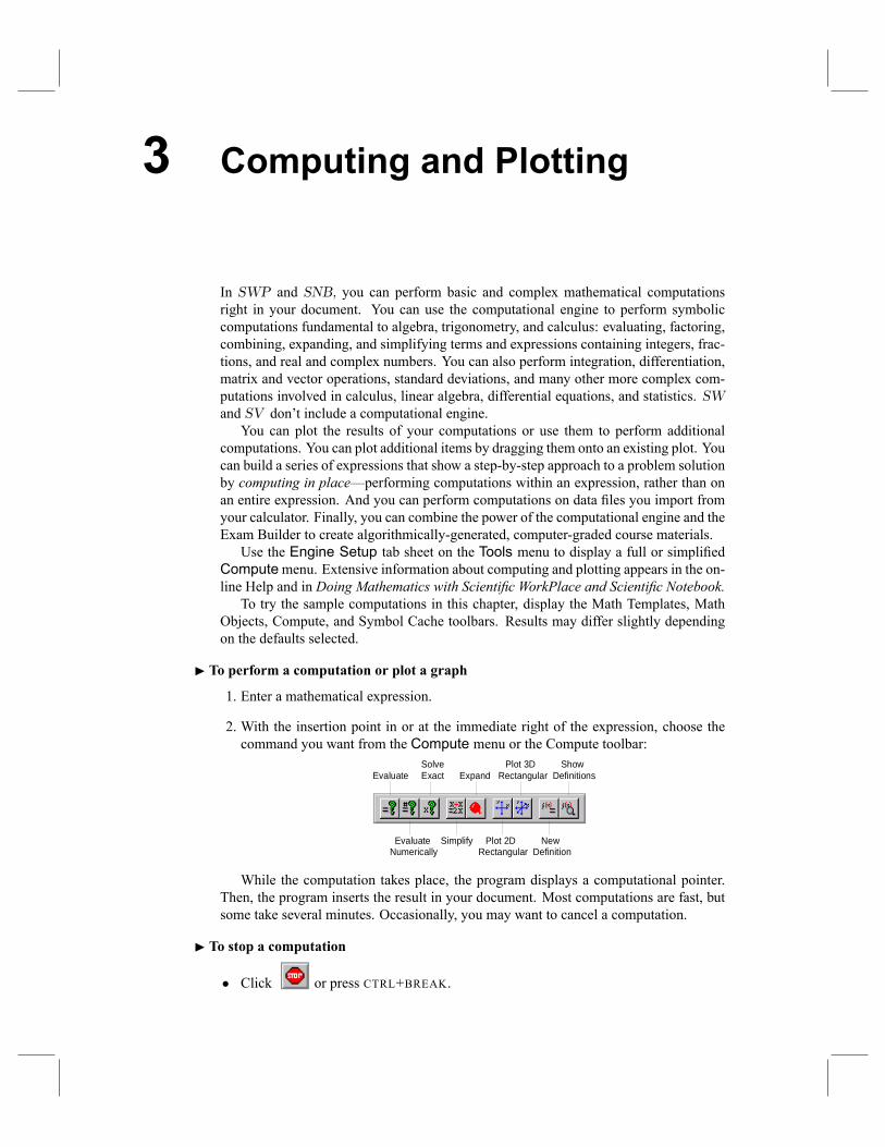
2. With the insertion point in or at the immediate right of the expression, choose thecommand you want from the Compute menu or the Compute toolbar:
Solve Plot 3D ShowEvaluate Exact Expand Rectangular Definitions
Evaluate Simplify Plot 2D NewNumerically Rectangular Definition
While the computation takes place, the program displays a computational pointer.Then, the program inserts the result in your document. Most computations are fast, butsome take several minutes. Occasionally, you may want to cancel a computation.
I To stop a computation
� Click or press CTRL+BREAK.
40 Chapter 3 Computing and Plotting
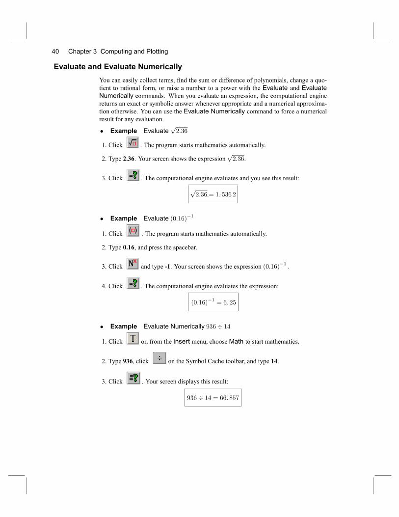
Evaluate and Evaluate NumericallyYou can easily collect terms, �nd the sum or difference of polynomials, change a quo-tient to rational form, or raise a number to a power with the Evaluate and EvaluateNumerically commands. When you evaluate an expression, the computational enginereturns an exact or symbolic answer whenever appropriate and a numerical approxima-tion otherwise. You can use the Evaluate Numerically command to force a numericalresult for any evaluation.
� Example Evaluatep2:36
1. Click . The program starts mathematics automatically.
2. Type 2.36. Your screen shows the expressionp2:36:
3. Click . The computational engine evaluates and you see this result:
p2:36.= 1: 536 2
� Example Evaluate (0:16)�1
1. Click . The program starts mathematics automatically.
2. Type 0.16, and press the spacebar.
3. Click and type -1. Your screen shows the expression (0:16)�1 :
4. Click . The computational engine evaluates the expression:
(0:16)�1= 6: 25
� Example Evaluate Numerically 936� 14
1. Click or, from the Insert menu, chooseMath to start mathematics.
2. Type 936, click on the Symbol Cache toolbar, and type 14.
3. Click . Your screen displays this result:
936� 14 = 66: 857
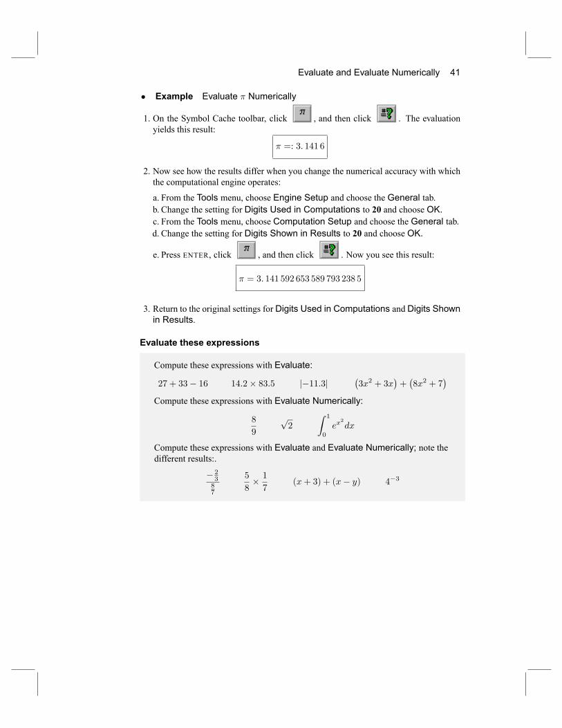
Evaluate and Evaluate Numerically 41
� Example Evaluate � Numerically
1. On the Symbol Cache toolbar, click , and then click . The evaluationyields this result:
� =: 3: 141 6
2. Now see how the results differ when you change the numerical accuracy with whichthe computational engine operates:
a. From the Tools menu, choose Engine Setup and choose the General tab.b. Change the setting for Digits Used in Computations to 20 and choose OK.c. From the Tools menu, choose Computation Setup and choose the General tab.d. Change the setting for Digits Shown in Results to 20 and choose OK.
e. Press ENTER, click , and then click . Now you see this result:
� = 3: 141 592 653 589 793 238 5
3. Return to the original settings for Digits Used in Computations and Digits Shownin Results.
Evaluate these expressions
Compute these expressions with Evaluate:
27 + 33� 16 14:2� 83:5 j�11:3j�3x2 + 3x
�+�8x2 + 7
�Compute these expressions with Evaluate Numerically:
8
9
p2
Z 1
0
ex2
dx
Compute these expressions with Evaluate and Evaluate Numerically; note thedifferent results:.
� 2387
5
8� 17
(x+ 3) + (x� y) 4�3
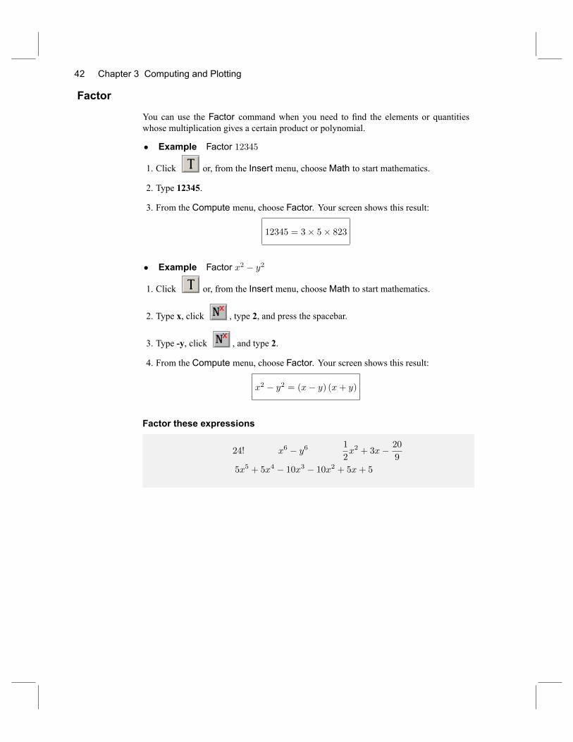
42 Chapter 3 Computing and Plotting
Factor
You can use the Factor command when you need to �nd the elements or quantitieswhose multiplication gives a certain product or polynomial.
� Example Factor 12345
1. Click or, from the Insert menu, chooseMath to start mathematics.
2. Type 12345.
3. From the Compute menu, choose Factor. Your screen shows this result:
12345 = 3� 5� 823
� Example Factor x2 � y2
1. Click or, from the Insert menu, chooseMath to start mathematics.
2. Type x, click , type 2, and press the spacebar.
3. Type -y, click , and type 2.
4. From the Compute menu, choose Factor. Your screen shows this result:
x2 � y2 = (x� y) (x+ y)
Factor these expressions
24! x6 � y6 1
2x2 + 3x� 20
9
5x5 + 5x4 � 10x3 � 10x2 + 5x+ 5
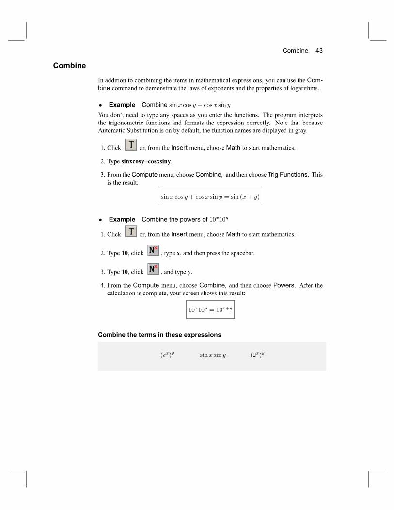
Combine 43
Combine
In addition to combining the items in mathematical expressions, you can use the Com-bine command to demonstrate the laws of exponents and the properties of logarithms.
� Example Combine sinx cos y + cosx sin yYou don't need to type any spaces as you enter the functions. The program interpretsthe trigonometric functions and formats the expression correctly. Note that becauseAutomatic Substitution is on by default, the function names are displayed in gray.
1. Click or, from the Insert menu, chooseMath to start mathematics.
2. Type sinxcosy+cosxsiny.
3. From theComputemenu, chooseCombine, and then choose Trig Functions. Thisis the result:
sinx cos y + cosx sin y = sin (x+ y)
� Example Combine the powers of 10x10y
1. Click or, from the Insert menu, chooseMath to start mathematics.
2. Type 10, click , type x, and then press the spacebar.
3. Type 10, click , and type y.
4. From the Compute menu, choose Combine, and then choose Powers. After thecalculation is complete, your screen shows this result:
10x10y = 10x+y
Combine the terms in these expressions
(ex)y
sinx sin y (2x)y
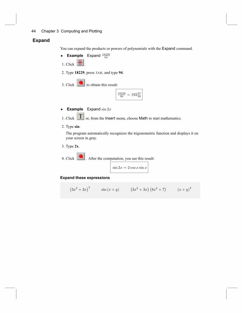
44 Chapter 3 Computing and Plotting
ExpandYou can expand the products or powers of polynomials with the Expand command.
� Example Expand 1822994
1. Click .
2. Type 18229, press TAB, and type 94.
3. Click to obtain this result:
1822994 = 193 8794
� Example Expand sin 2x
1. Click or, from the Insert menu, chooseMath to start mathematics.
2. Type sin.
The program automatically recognizes the trigonometric function and displays it onyour screen in gray.
3. Type 2x.
4. Click . After the computation, you see this result:
sin 2x = 2 cosx sinx
Expand these expressions
�3x2 + 3x
�3sin (x+ y)
�3x2 + 3x
� �8x2 + 7
�(x+ y)
4
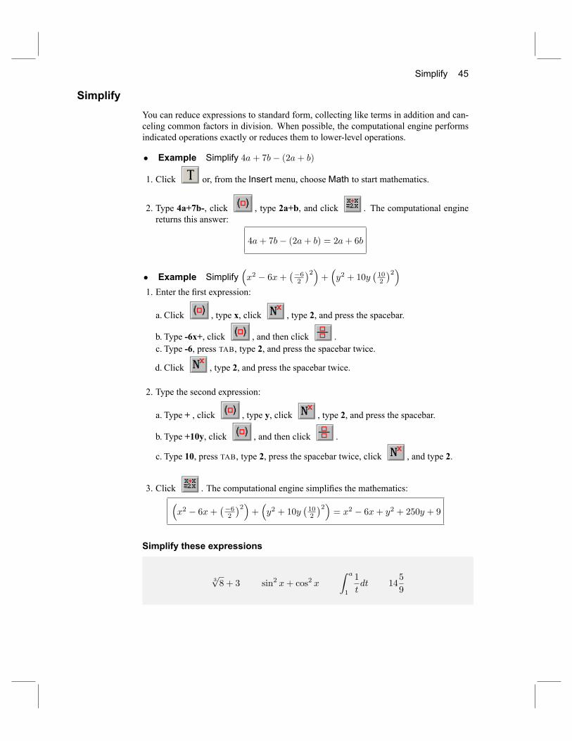
Simplify 45
SimplifyYou can reduce expressions to standard form, collecting like terms in addition and can-celing common factors in division. When possible, the computational engine performsindicated operations exactly or reduces them to lower-level operations.
� Example Simplify 4a+ 7b� (2a+ b)
1. Click or, from the Insert menu, chooseMath to start mathematics.
2. Type 4a+7b-, click , type 2a+b, and click . The computational enginereturns this answer:
4a+ 7b� (2a+ b) = 2a+ 6b
� Example Simplify�x2 � 6x+
��62
�2�+�y2 + 10y
�102
�2�1. Enter the �rst expression:
a. Click , type x, click , type 2, and press the spacebar.
b. Type -6x+, click , and then click .c. Type -6, press TAB, type 2, and press the spacebar twice.
d. Click , type 2, and press the spacebar twice.
2. Type the second expression:
a. Type + , click , type y, click , type 2, and press the spacebar.
b. Type +10y, click , and then click .
c. Type 10, press TAB, type 2, press the spacebar twice, click , and type 2.
3. Click . The computational engine simpli�es the mathematics:�x2 � 6x+
��62
�2�+�y2 + 10y
�102
�2�= x2 � 6x+ y2 + 250y + 9
Simplify these expressions
3p8 + 3 sin2 x+ cos2 x
Z a
1
1
tdt 14
5
9
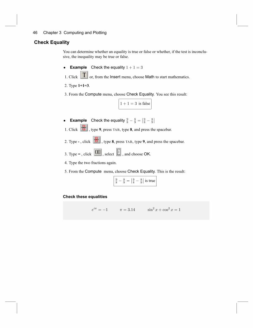
46 Chapter 3 Computing and Plotting
Check Equality
You can determine whether an equality is true or false or whether, if the test is inconclu-sive, the inequality may be true or false.
� Example Check the equality 1 + 1 = 3
1. Click or, from the Insert menu, chooseMath to start mathematics.
2. Type 1+1=3.
3. From the Compute menu, choose Check Equality. You see this result:
1 + 1 = 3 is false
� Example Check the equality 98 �
89 =
�� 98 �
89
��1. Click , type 9, press TAB, type 8, and press the spacebar.
2. Type - , click , type 8, press TAB, type 9, and press the spacebar.
3. Type = , click , select , and choose OK.
4. Type the two fractions again.
5. From the Compute menu, choose Check Equality. This is the result:
98 �
89 =
�� 98 �
89
�� is trueCheck these equalities
ei� = �1 � = 3:14 sin2 x+ cos2 x = 1
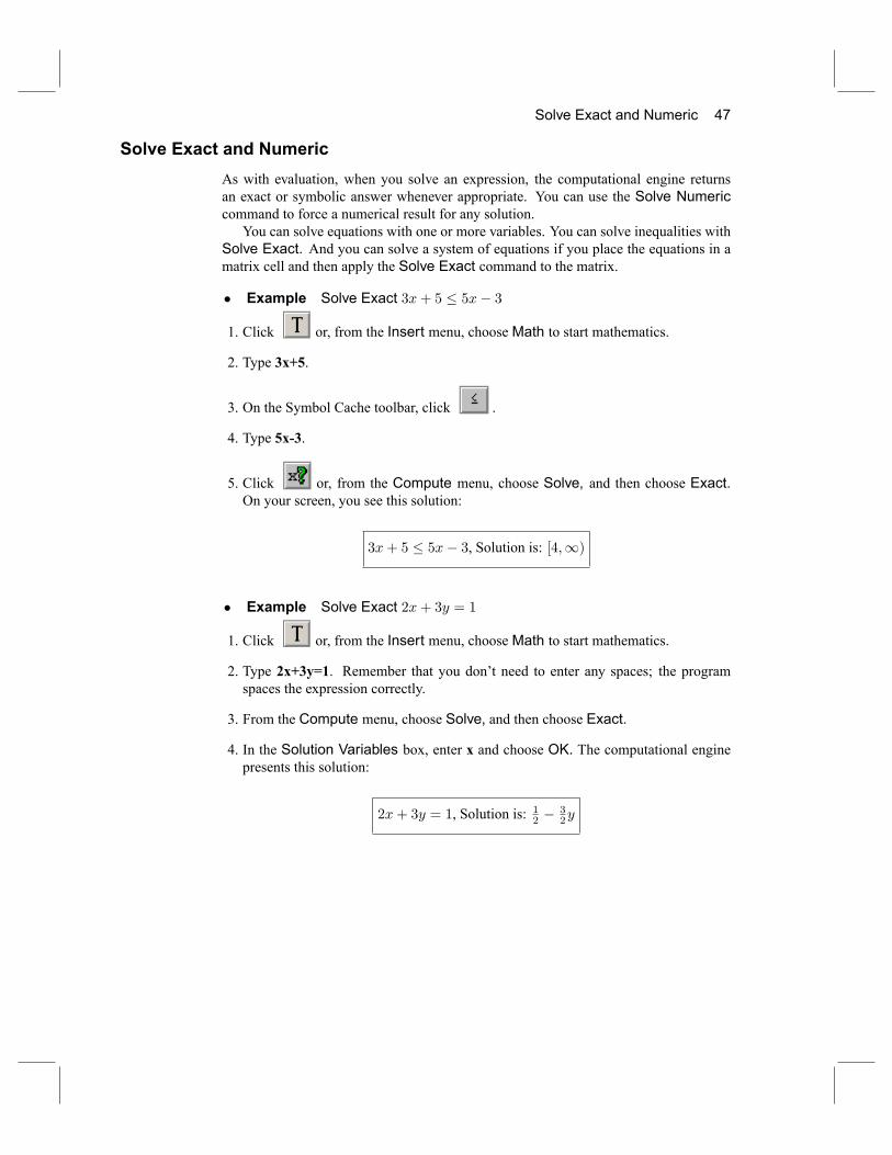
Solve Exact and Numeric 47
Solve Exact and NumericAs with evaluation, when you solve an expression, the computational engine returnsan exact or symbolic answer whenever appropriate. You can use the Solve Numericcommand to force a numerical result for any solution.You can solve equations with one or more variables. You can solve inequalities with
Solve Exact. And you can solve a system of equations if you place the equations in amatrix cell and then apply the Solve Exact command to the matrix.
� Example Solve Exact 3x+ 5 � 5x� 3
1. Click or, from the Insert menu, chooseMath to start mathematics.
2. Type 3x+5.
3. On the Symbol Cache toolbar, click .
4. Type 5x-3.
5. Click or, from the Compute menu, choose Solve, and then choose Exact.On your screen, you see this solution:
3x+ 5 � 5x� 3, Solution is: [4;1)
� Example Solve Exact 2x+ 3y = 1
1. Click or, from the Insert menu, chooseMath to start mathematics.
2. Type 2x+3y=1. Remember that you don't need to enter any spaces; the programspaces the expression correctly.
3. From the Compute menu, choose Solve, and then choose Exact.
4. In the Solution Variables box, enter x and choose OK. The computational enginepresents this solution:
2x+ 3y = 1, Solution is: 12 �32y
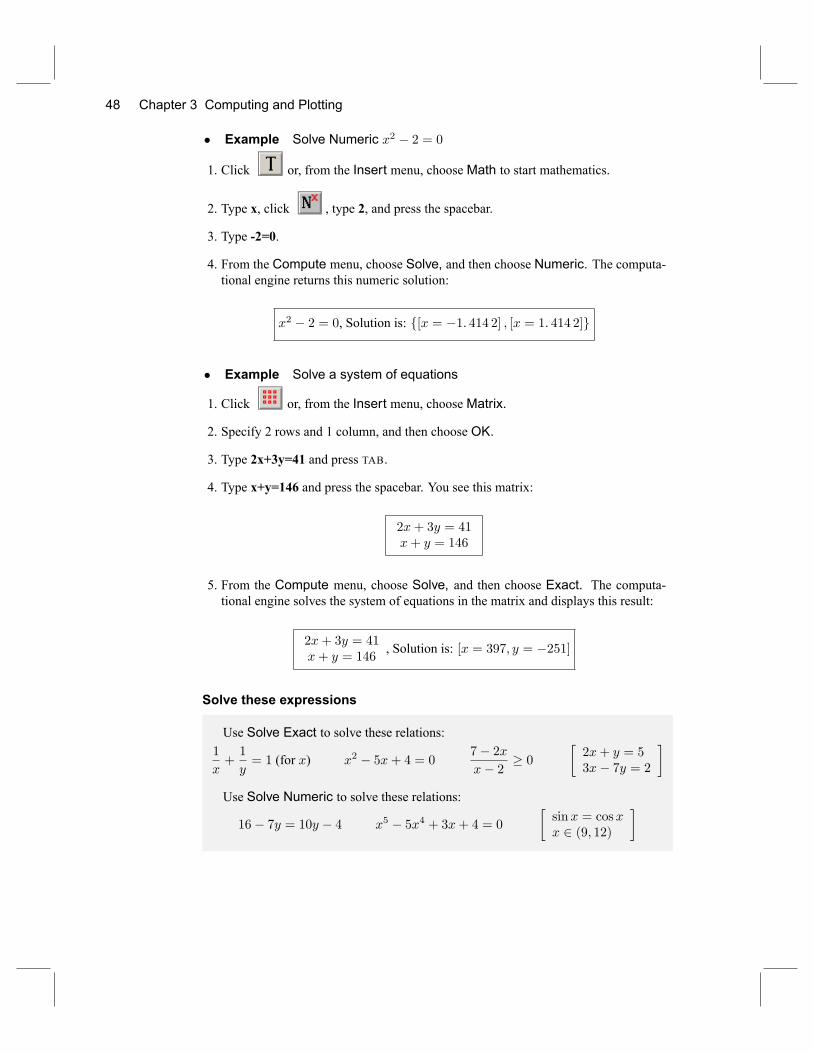
48 Chapter 3 Computing and Plotting
� Example Solve Numeric x2 � 2 = 0
1. Click or, from the Insert menu, chooseMath to start mathematics.
2. Type x, click , type 2, and press the spacebar.
3. Type -2=0.
4. From the Compute menu, choose Solve, and then choose Numeric. The computa-tional engine returns this numeric solution:
x2 � 2 = 0, Solution is: f[x = �1: 414 2] ; [x = 1: 414 2]g
� Example Solve a system of equations
1. Click or, from the Insert menu, chooseMatrix.
2. Specify 2 rows and 1 column, and then choose OK.
3. Type 2x+3y=41 and press TAB.
4. Type x+y=146 and press the spacebar. You see this matrix:
2x+ 3y = 41x+ y = 146
5. From the Compute menu, choose Solve, and then choose Exact. The computa-tional engine solves the system of equations in the matrix and displays this result:
2x+ 3y = 41x+ y = 146
, Solution is: [x = 397; y = �251]
Solve these expressions
Use Solve Exact to solve these relations:1
x+1
y= 1 (for x) x2 � 5x+ 4 = 0 7� 2x
x� 2 � 0�2x+ y = 53x� 7y = 2
�Use Solve Numeric to solve these relations:
16� 7y = 10y � 4 x5 � 5x4 + 3x+ 4 = 0�sinx = cosxx 2 (9; 12)
�
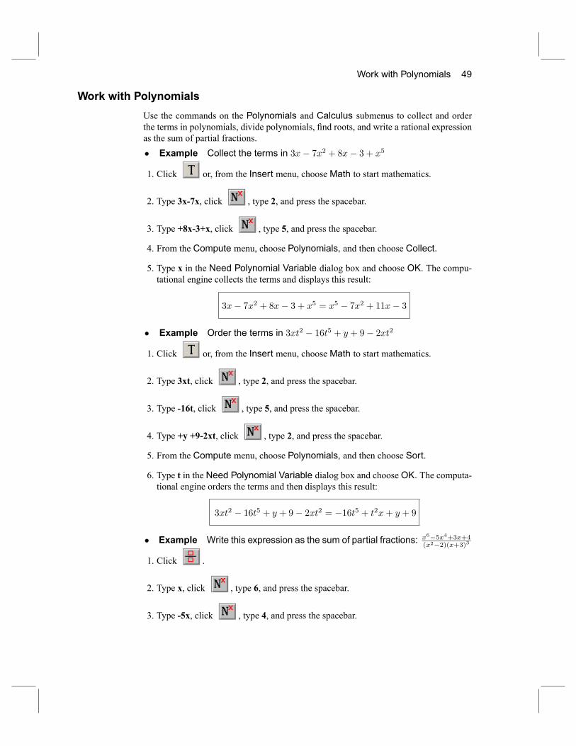
Work with Polynomials 49
Work with PolynomialsUse the commands on the Polynomials and Calculus submenus to collect and orderthe terms in polynomials, divide polynomials, �nd roots, and write a rational expressionas the sum of partial fractions.� Example Collect the terms in 3x� 7x2 + 8x� 3 + x5
1. Click or, from the Insert menu, chooseMath to start mathematics.
2. Type 3x-7x, click , type 2, and press the spacebar.
3. Type +8x-3+x, click , type 5, and press the spacebar.
4. From the Compute menu, choose Polynomials, and then choose Collect.
5. Type x in the Need Polynomial Variable dialog box and choose OK. The compu-tational engine collects the terms and displays this result:
3x� 7x2 + 8x� 3 + x5 = x5 � 7x2 + 11x� 3
� Example Order the terms in 3xt2 � 16t5 + y + 9� 2xt2
1. Click or, from the Insert menu, chooseMath to start mathematics.
2. Type 3xt, click , type 2, and press the spacebar.
3. Type -16t, click , type 5, and press the spacebar.
4. Type +y +9-2xt, click , type 2, and press the spacebar.
5. From the Compute menu, choose Polynomials, and then choose Sort.
6. Type t in the Need Polynomial Variable dialog box and choose OK. The computa-tional engine orders the terms and then displays this result:
3xt2 � 16t5 + y + 9� 2xt2 = �16t5 + t2x+ y + 9
� Example Write this expression as the sum of partial fractions: x6�5x4+3x+4(x2�2)(x+3)3
1. Click .
2. Type x, click , type 6, and press the spacebar.
3. Type -5x, click , type 4, and press the spacebar.
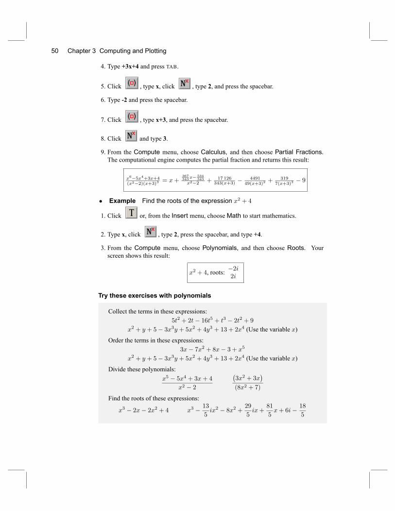
50 Chapter 3 Computing and Plotting
4. Type +3x+4 and press TAB.
5. Click , type x, click , type 2, and press the spacebar.
6. Type -2 and press the spacebar.
7. Click , type x+3, and press the spacebar.
8. Click and type 3.
9. From the Compute menu, choose Calculus, and then choose Partial Fractions.The computational engine computes the partial fraction and returns this result:
x6�5x4+3x+4(x2�2)(x+3)3 = x+
367343x�
534343
x2�2 + 17 126343(x+3) �
449149(x+3)2
+ 3197(x+3)3
� 9
� Example Find the roots of the expression x2 + 4
1. Click or, from the Insert menu, chooseMath to start mathematics.
2. Type x, click , type 2, press the spacebar, and type +4.
3. From the Compute menu, choose Polynomials, and then choose Roots. Yourscreen shows this result:
x2 + 4, roots: �2i2i
Try these exercises with polynomials
Collect the terms in these expressions:5t2 + 2t� 16t5 + t3 � 2t2 + 9
x2 + y + 5� 3x3y + 5x2 + 4y3 + 13 + 2x4 (Use the variable x)Order the terms in these expressions:
3x� 7x2 + 8x� 3 + x5
x2 + y + 5� 3x3y + 5x2 + 4y3 + 13 + 2x4 (Use the variable x)Divide these polynomials:
x5 � 5x4 + 3x+ 4x2 � 2
�3x2 + 3x
�(8x2 + 7)
Find the roots of these expressions:
x3 � 2x� 2x2 + 4 x3 � 135ix2 � 8x2 + 29
5ix+
81
5x+ 6i� 18
5
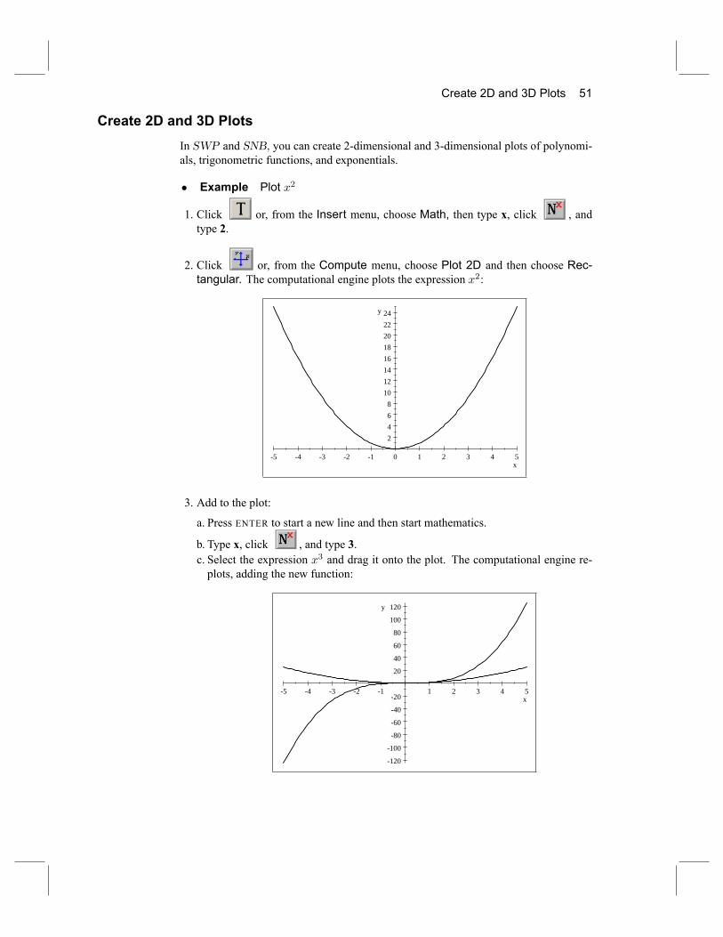
Create 2D and 3D Plots 51
Create 2D and 3D PlotsIn SWP and SNB, you can create 2-dimensional and 3-dimensional plots of polynomi-als, trigonometric functions, and exponentials.
� Example Plot x2
1. Click or, from the Insert menu, choose Math, then type x, click , andtype 2.
2. Click or, from the Compute menu, choose Plot 2D and then choose Rec-tangular. The computational engine plots the expression x2:
5 4 3 2 1 0 1 2 3 4 5
2468
1012141618202224
x
y
3. Add to the plot:
a. Press ENTER to start a new line and then start mathematics.
b. Type x, click , and type 3.c. Select the expression x3 and drag it onto the plot. The computational engine re-plots, adding the new function:
5 4 3 2 1 1 2 3 4 5
120
100
80
60
40
20
20
40
60
80
100
120
x
y
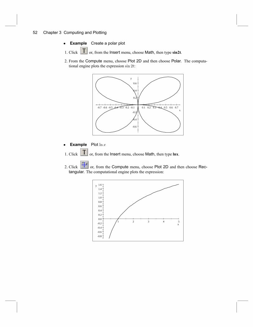
52 Chapter 3 Computing and Plotting
� Example Create a polar plot
1. Click or, from the Insert menu, chooseMath, then type sin2t.
2. From the Compute menu, choose Plot 2D and then choose Polar. The computa-tional engine plots the expression sin 2t:
0.7 0.6 0.5 0.4 0.3 0.2 0.1 0.1 0.2 0.3 0.4 0.5 0.6 0.7
0.6
0.4
0.2
0.2
0.4
0.6
x
y
� Example Plot lnx
1. Click or, from the Insert menu, chooseMath, then type lnx.
2. Click or, from the Compute menu, choose Plot 2D and then choose Rec-tangular. The computational engine plots the expression:
1 2 3 4 5
0.8
0.6
0.4
0.2
0.0
0.2
0.4
0.6
0.8
1.0
1.2
1.4
1.6
x
y
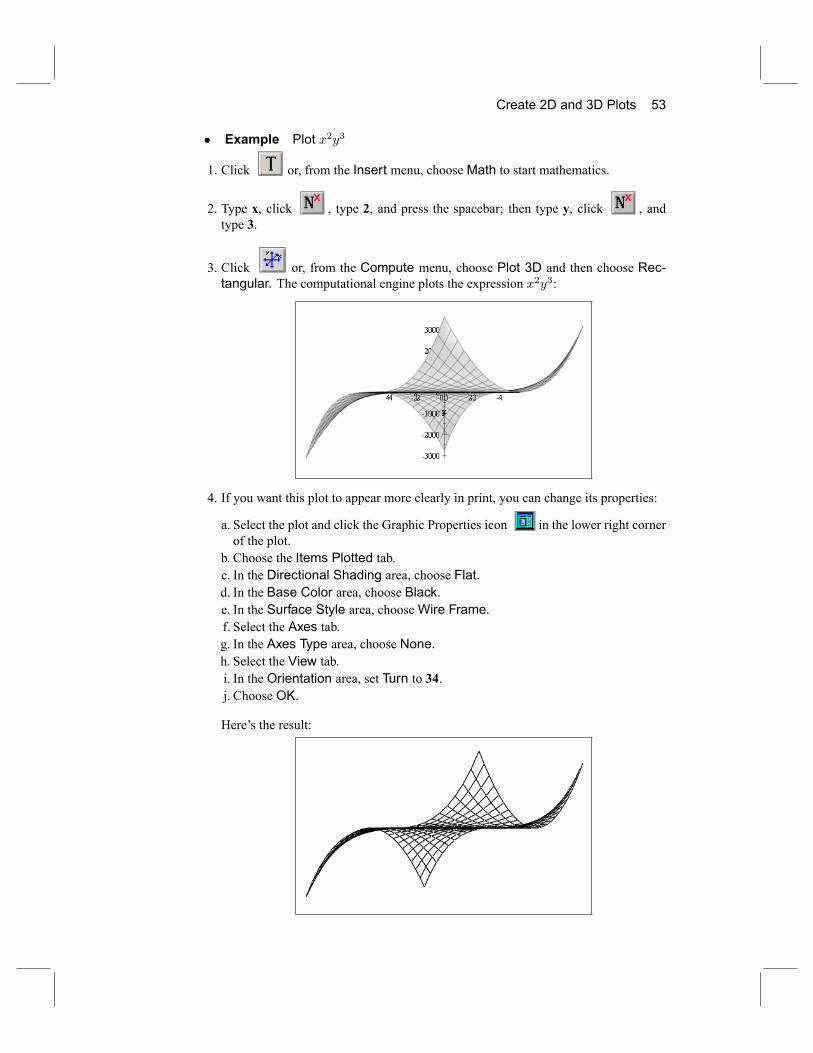
Create 2D and 3D Plots 53
� Example Plot x2y3
1. Click or, from the Insert menu, chooseMath to start mathematics.
2. Type x, click , type 2, and press the spacebar; then type y, click , andtype 3.
3. Click or, from the Compute menu, choose Plot 3D and then choose Rec-tangular. The computational engine plots the expression x2y3:
4. If you want this plot to appear more clearly in print, you can change its properties:
a. Select the plot and click the Graphic Properties icon in the lower right cornerof the plot.
b. Choose the Items Plotted tab.c. In the Directional Shading area, choose Flat.d. In the Base Color area, choose Black.e. In the Surface Style area, chooseWire Frame.f. Select the Axes tab.g. In the Axes Type area, choose None.h. Select the View tab.i. In the Orientation area, set Turn to 34.j. Choose OK.
Here's the result:
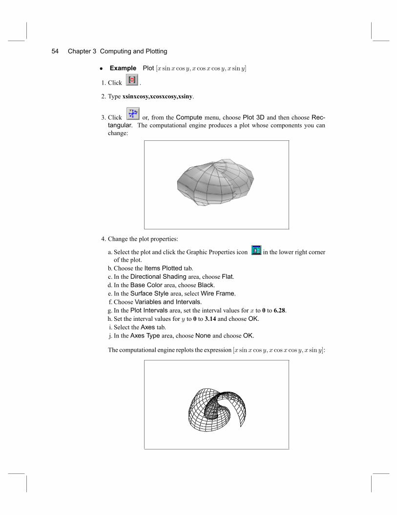
54 Chapter 3 Computing and Plotting
� Example Plot [x sinx cos y; x cosx cos y; x sin y]
1. Click .
2. Type xsinxcosy,xcosxcosy,xsiny.
3. Click or, from the Compute menu, choose Plot 3D and then choose Rec-tangular. The computational engine produces a plot whose components you canchange:
4. Change the plot properties:
a. Select the plot and click the Graphic Properties icon in the lower right cornerof the plot.
b. Choose the Items Plotted tab.c. In the Directional Shading area, choose Flat.d. In the Base Color area, choose Black.e. In the Surface Style area, selectWire Frame.f. Choose Variables and Intervals.g. In the Plot Intervals area, set the interval values for x to 0 to 6.28.h. Set the interval values for y to 0 to 3.14 and choose OK.i. Select the Axes tab.j. In the Axes Type area, choose None and choose OK.
The computational engine replots the expression [x sinx cos y; x cosx cos y; x sin y]:
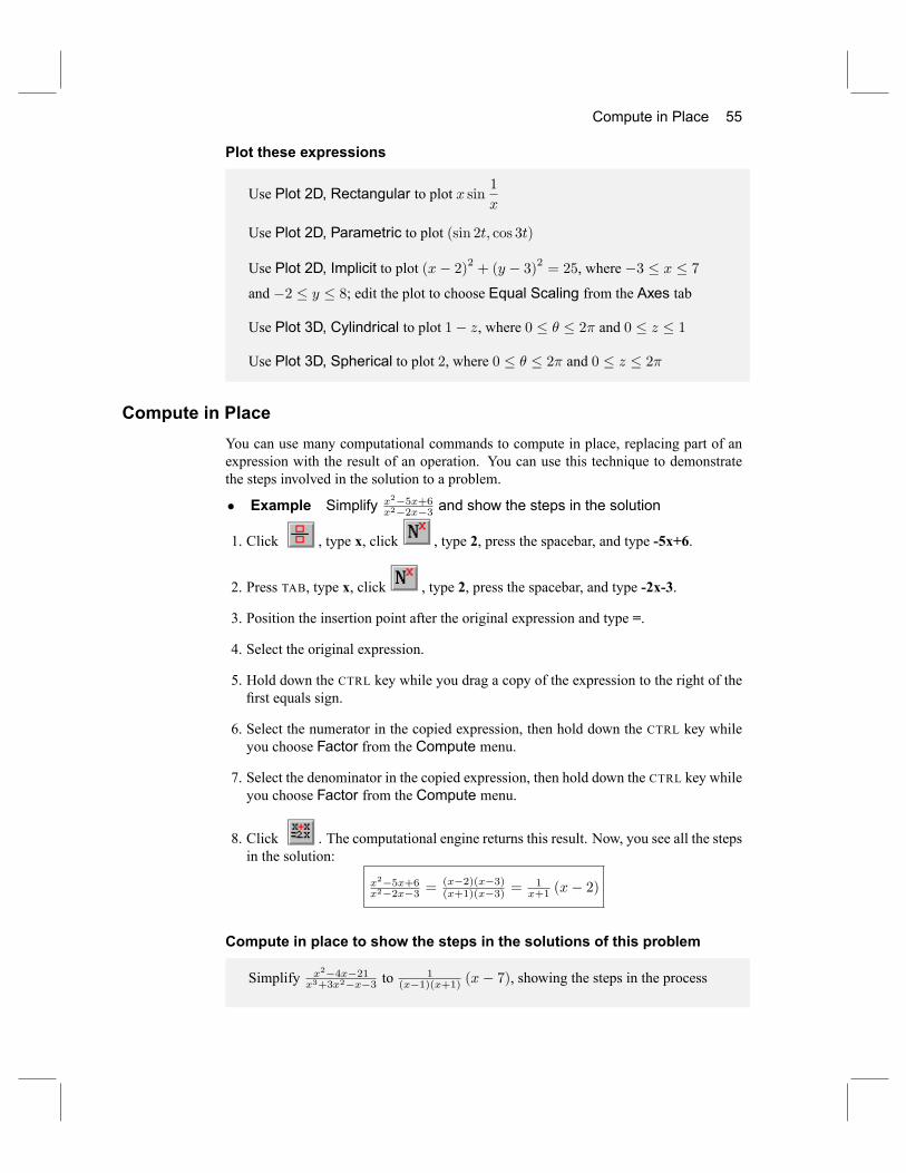
Compute in Place 55
Plot these expressions
Use Plot 2D, Rectangular to plot x sin1
x
Use Plot 2D, Parametric to plot (sin 2t; cos 3t)
Use Plot 2D, Implicit to plot (x� 2)2 + (y � 3)2 = 25, where �3 � x � 7and �2 � y � 8; edit the plot to choose Equal Scaling from the Axes tab
Use Plot 3D, Cylindrical to plot 1� z, where 0 � � � 2� and 0 � z � 1
Use Plot 3D, Spherical to plot 2, where 0 � � � 2� and 0 � z � 2�
Compute in PlaceYou can use many computational commands to compute in place, replacing part of anexpression with the result of an operation. You can use this technique to demonstratethe steps involved in the solution to a problem.
� Example Simplify x2�5x+6x2�2x�3 and show the steps in the solution
1. Click , type x, click , type 2, press the spacebar, and type -5x+6.
2. Press TAB, type x, click , type 2, press the spacebar, and type -2x-3.
3. Position the insertion point after the original expression and type =.
4. Select the original expression.
5. Hold down the CTRL key while you drag a copy of the expression to the right of the�rst equals sign.
6. Select the numerator in the copied expression, then hold down the CTRL key whileyou choose Factor from the Compute menu.
7. Select the denominator in the copied expression, then hold down the CTRL key whileyou choose Factor from the Compute menu.
8. Click . The computational engine returns this result. Now, you see all the stepsin the solution:
x2�5x+6x2�2x�3 =
(x�2)(x�3)(x+1)(x�3) =
1x+1 (x� 2)
Compute in place to show the steps in the solutions of this problem
Simplify x2�4x�21x3+3x2�x�3 to
1(x�1)(x+1) (x� 7), showing the steps in the process
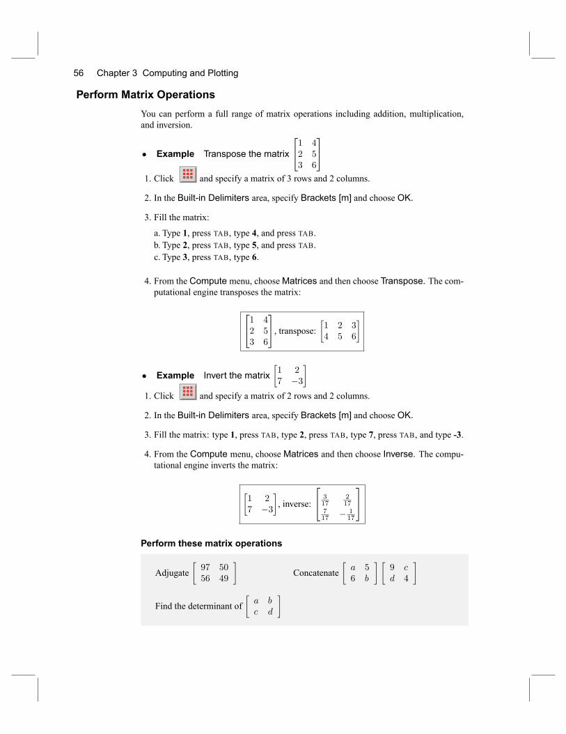
56 Chapter 3 Computing and Plotting
Perform Matrix OperationsYou can perform a full range of matrix operations including addition, multiplication,and inversion.
� Example Transpose the matrix
241 42 53 6
351. Click and specify a matrix of 3 rows and 2 columns.
2. In the Built-in Delimiters area, specify Brackets [m] and choose OK.
3. Fill the matrix:
a. Type 1, press TAB, type 4, and press TAB.b. Type 2, press TAB, type 5, and press TAB.c. Type 3, press TAB, type 6.
4. From the Compute menu, chooseMatrices and then choose Transpose. The com-putational engine transposes the matrix:
241 42 53 6
35, transpose: �1 2 34 5 6
�
� Example Invert the matrix�1 27 �3
�1. Click and specify a matrix of 2 rows and 2 columns.
2. In the Built-in Delimiters area, specify Brackets [m] and choose OK.
3. Fill the matrix: type 1, press TAB, type 2, press TAB, type 7, press TAB, and type -3.
4. From the Compute menu, choose Matrices and then choose Inverse. The compu-tational engine inverts the matrix:
�1 27 �3
�, inverse:
24 317
217
717 � 1
17
35Perform these matrix operations
Adjugate�97 5056 49
�Concatenate
�a 56 b
� �9 cd 4
�
Find the determinant of�a bc d
�
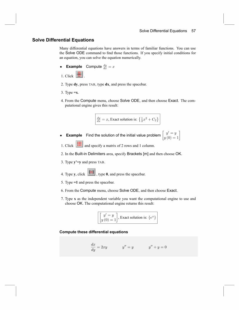
Solve Differential Equations 57
Solve Differential EquationsMany differential equations have answers in terms of familiar functions. You can usethe Solve ODE command to �nd those functions. If you specify initial conditions foran equation, you can solve the equation numerically.
� Example Compute dydx = x
1. Click .
2. Type dy, press TAB, type dx, and press the spacebar.
3. Type =x.
4. From the Compute menu, choose Solve ODE, and then choose Exact. The com-putational engine gives this result:
dydx = x, Exact solution is:
�12x
2 + C2
� Example Find the solution of the initial value problem�y0 = yy (0) = 1
�1. Click and specify a matrix of 2 rows and 1 column.
2. In the Built-in Delimiters area, specify Brackets [m] and then choose OK.
3. Type y'=y and press TAB.
4. Type y, click , type 0, and press the spacebar.
5. Type =1 and press the spacebar.
6. From the Compute menu, choose Solve ODE, and then choose Exact.
7. Type x as the independent variable you want the computational engine to use andchoose OK. The computational engine returns this result:
�y0 = yy (0) = 1
�, Exact solution is: fexg
Compute these differential equations
dx
dy= 2xy y00 = y y00 + y = 0
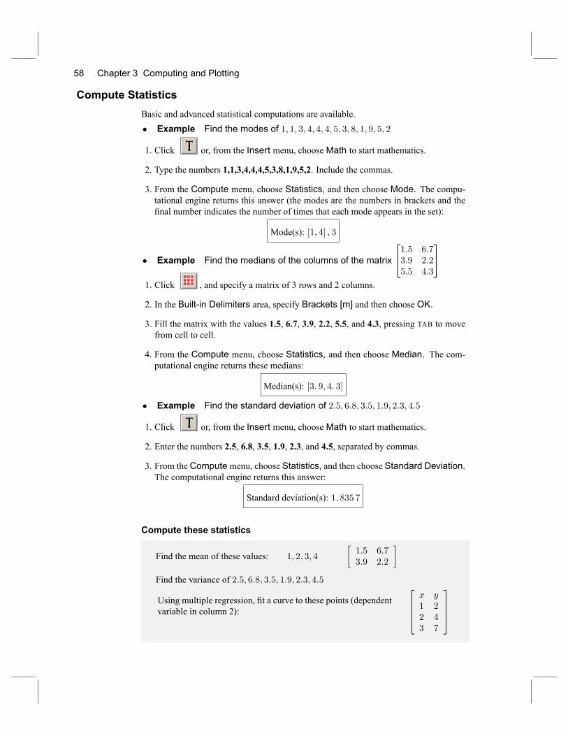
58 Chapter 3 Computing and Plotting
Compute StatisticsBasic and advanced statistical computations are available.� Example Find the modes of 1; 1; 3; 4; 4; 4; 5; 3; 8; 1; 9; 5; 2
1. Click or, from the Insert menu, chooseMath to start mathematics.
2. Type the numbers 1,1,3,4,4,4,5,3,8,1,9,5,2. Include the commas.
3. From the Compute menu, choose Statistics, and then choose Mode. The compu-tational engine returns this answer (the modes are the numbers in brackets and the�nal number indicates the number of times that each mode appears in the set):
Mode(s): [1; 4] ; 3
� Example Find the medians of the columns of the matrix
241:5 6:73:9 2:25:5 4:3
351. Click , and specify a matrix of 3 rows and 2 columns.
2. In the Built-in Delimiters area, specify Brackets [m] and then choose OK.
3. Fill the matrix with the values 1.5, 6.7, 3.9, 2.2, 5.5, and 4.3, pressing TAB to movefrom cell to cell.
4. From the Compute menu, choose Statistics, and then choose Median. The com-putational engine returns these medians:
Median(s): [3: 9; 4: 3]
� Example Find the standard deviation of 2:5; 6:8; 3:5; 1:9; 2:3; 4:5
1. Click or, from the Insert menu, chooseMath to start mathematics.
2. Enter the numbers 2.5, 6.8, 3.5, 1.9, 2.3, and 4.5, separated by commas.
3. From theCompute menu, choose Statistics, and then choose Standard Deviation.The computational engine returns this answer:
Standard deviation(s): 1: 835 7
Compute these statistics
Find the mean of these values: 1; 2; 3; 4
�1:5 6:73:9 2:2
�Find the variance of 2:5; 6:8; 3:5; 1:9; 2:3; 4:5
Using multiple regression, �t a curve to these points (dependentvariable in column 2):
2664x y1 22 43 7
3775
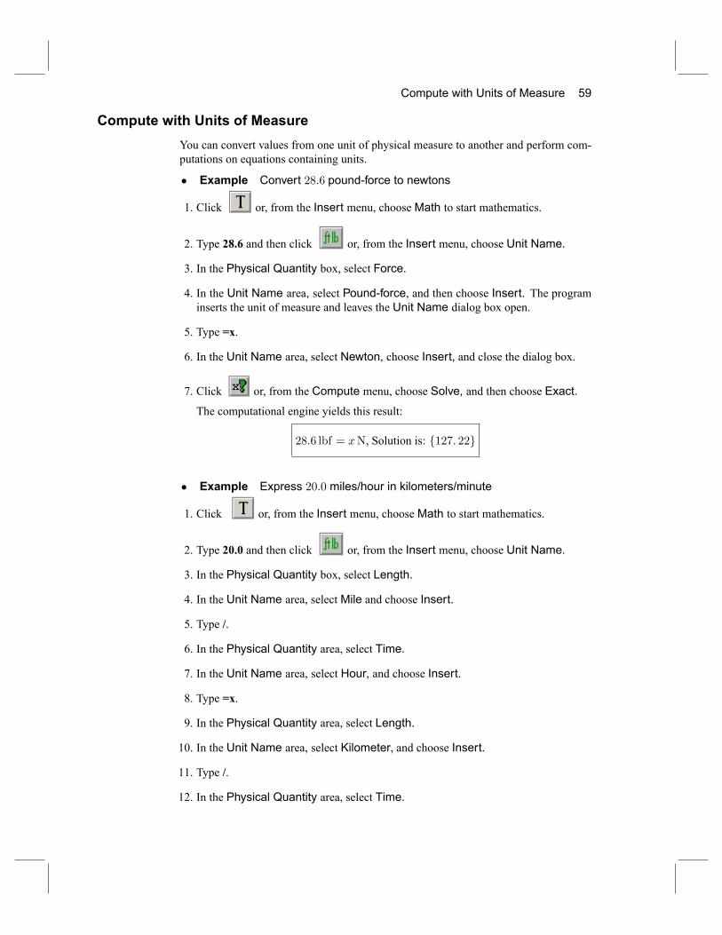
Compute with Units of Measure 59
Compute with Units of MeasureYou can convert values from one unit of physical measure to another and perform com-putations on equations containing units.
� Example Convert 28:6 pound-force to newtons
1. Click or, from the Insert menu, chooseMath to start mathematics.
2. Type 28.6 and then click or, from the Insert menu, choose Unit Name.
3. In the Physical Quantity box, select Force.
4. In the Unit Name area, select Pound-force, and then choose Insert. The programinserts the unit of measure and leaves the Unit Name dialog box open.
5. Type =x.
6. In the Unit Name area, select Newton, choose Insert, and close the dialog box.
7. Click or, from the Compute menu, choose Solve, and then choose Exact.
The computational engine yields this result:
28:6 lbf = xN, Solution is: f127: 22g
� Example Express 20:0 miles/hour in kilometers/minute
1. Click or, from the Insert menu, chooseMath to start mathematics.
2. Type 20.0 and then click or, from the Insert menu, choose Unit Name.
3. In the Physical Quantity box, select Length.
4. In the Unit Name area, selectMile and choose Insert.
5. Type /.
6. In the Physical Quantity area, select Time.
7. In the Unit Name area, select Hour, and choose Insert.
8. Type =x.
9. In the Physical Quantity area, select Length.
10. In the Unit Name area, select Kilometer, and choose Insert.
11. Type /.
12. In the Physical Quantity area, select Time.
60 Chapter 3 Computing and Plotting
13. In the Unit Name area, selectMinute, and choose Insert and close the dialog box.
14. Click or, from the Compute menu, choose Solve and then choose Exact.This is the result:
20:0mi=h = x km=min, Solution is: 0:536 45
Compute these conversions
Express 53:7 lbf= in2 in newtons per square meter
Compute 3A6V and then convert the answer to watts
Convert 3:7N= cm2 to pounds per square inch
Create Exams and QuizzesIn SWP and SNB, you can create algorithmically-generated course materials such asexams, quizzes, tests, tutorials, problem sets, drills, and homework assignments. Insteadof writing a series of exams, each containing a variation of your questions and answers,you can use the Exam Builder to write a single exam and state the questions and answerswith algorithms. Students can drill and practice a skill at length by opening the sameExam Builder �le repeatedly, obtaining a different set of questions each time. Similarly,you can test each student with a different version of an exam, with each version drawnfrom the same Exam Builder source �le.The Exam Builder is appropriate for any level of mathematics instruction�elemen-
tary arithmetic, algebra, trigonometry, calculus, linear algebra, differential equations,probability, or statistics. Course materials created with the Exam Builder can be workedand graded online or in the traditional pencil-and-paper form. The online Help systemcontains detailed instructions for using the Exam Builder.You can �nd many sample quizzes in the Quizzes directory of your program in-
stallation. These instructions explain how to open and take one of the sample exams.
I To open a quiz1. Open SWP or SNB and from the File menu, choose Open.
2. Specify the Quizzes directory of your program installation.
3. In the Files of type box, choose Quiz (*.qiz).
4. Select one of the �les in the directory and choose OK to open the sample exam.
5. Enter your name on the exam and answer each question.
6. Choose Click to grade. The program grades the exam and opens a �le containingthe results.
7. Open the same .qiz �le again and note that the program has automatically generateda different set of questions.
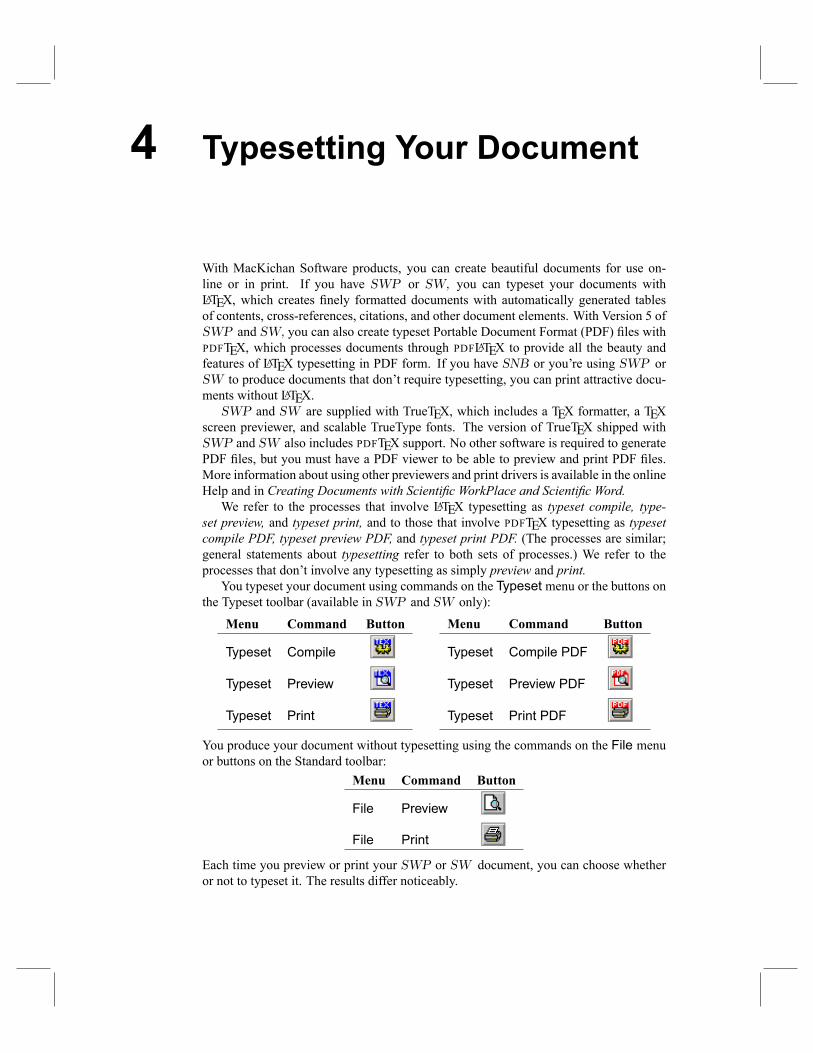
4 Typesetting Your Document
With MacKichan Software products, you can create beautiful documents for use on-line or in print. If you have SWP or SW, you can typeset your documents withLATEX, which creates �nely formatted documents with automatically generated tablesof contents, cross-references, citations, and other document elements. With Version 5 ofSWP and SW, you can also create typeset Portable Document Format (PDF) �les withPDFTEX, which processes documents through PDFLATEX to provide all the beauty andfeatures of LATEX typesetting in PDF form. If you have SNB or you're using SWP orSW to produce documents that don't require typesetting, you can print attractive docu-ments without LATEX.SWP and SW are supplied with TrueTEX, which includes a TEX formatter, a TEX
screen previewer, and scalable TrueType fonts. The version of TrueTEX shipped withSWP and SW also includes PDFTEX support. No other software is required to generatePDF �les, but you must have a PDF viewer to be able to preview and print PDF �les.More information about using other previewers and print drivers is available in the onlineHelp and in Creating Documents with Scienti�c WorkPlace and Scienti�c Word.We refer to the processes that involve LATEX typesetting as typeset compile, type-
set preview, and typeset print, and to those that involve PDFTEX typesetting as typesetcompile PDF, typeset preview PDF, and typeset print PDF. (The processes are similar;general statements about typesetting refer to both sets of processes.) We refer to theprocesses that don't involve any typesetting as simply preview and print.You typeset your document using commands on the Typeset menu or the buttons on
the Typeset toolbar (available in SWP and SW only):
Menu Command Button
Typeset Compile
Typeset Preview
Typeset Print
Menu Command Button
Typeset Compile PDF
Typeset Preview PDF
Typeset Print PDF
You produce your document without typesetting using the commands on the File menuor buttons on the Standard toolbar:
Menu Command Button
File Preview
File Print
Each time you preview or print your SWP or SW document, you can choose whetheror not to typeset it. The results differ noticeably.
62 Chapter 4 Typesetting Your Document
Understanding the Typesetting Process
When you typeset, the program compiles your document with LATEX or PDFLATEX. Thecompilation applies special LATEX formatting features to resolve typographic details suchas hyphenation, ligatures, line spacing, and line and page breaking. The process alsocreates automatic numbering, cross-references, citations, and footnotes. It generatesany document elements speci�ed in the document shell, such as a table of contents,bibliography, or index. Depending on the complexity of your document, the programmay process it through LATEX or PDFLATEX more than once. During the compilation,SWP and SW remain open, but they are suspended.The results of the compilation differ depending on whether you typeset your docu-
ment with LATEX or PDFLATEX. In either case, your original document is unchanged.� If you typeset with LATEX (using the Preview or Print commands on the Typesetmenu), the compilation yields a device independent, or DVI, �le that contains yourtypeset document in a form independent of any output device. The compilation mayalso result in other generated �les, such as table of contents �les or bibliography�les, that are required by the DVI �le.
� If you typeset with PDFLATEX (using the Preview PDF or Print PDF commandson the Typeset menu), the compilation yields a PDF �le that contains your typesetdocument embedded with all necessary fonts and graphics. If you have added thehyperref package to your document, the compilation creates hypertext links in placeof cross-references and links the table of contents to the rest of the document withhypertext links.
If you typeset with the Compile or Compile PDF command, the program compilesthe document and creates the DVI or PDF �le but doesn't preview or print it. Otherwise,following the compilation, the program previews or prints the �le, according to yourchoice. Because of the typesetting speci�cations and the features and elements addedduring compilation, the appearance of your document may be quite different from itsappearance in the document window.When you don't typeset your document, the program uses many of the same rou-
tines to preview and print as it does to display the document on the screen. The programdoesn't use special formatting features, nor does it automatically generate any docu-ment elements. Therefore, the appearance of the previewed or printed document is quitesimilar to its appearance in the document window.These general guidelines may help you decide which document production method
to use:� When a �nely typeset document appearance is a high priority, typeset preview ortypeset print the document with the commands on the Typeset menu.
� When you need a �nely typeset PDF document for viewing on multiple platforms,typeset the document with the PDF commands on the Typeset menu.
� When a �nely typeset document appearance and automatically generated documentelements aren't a priority or you need output quickly, preview or print the documentwith the commands on the File menu.
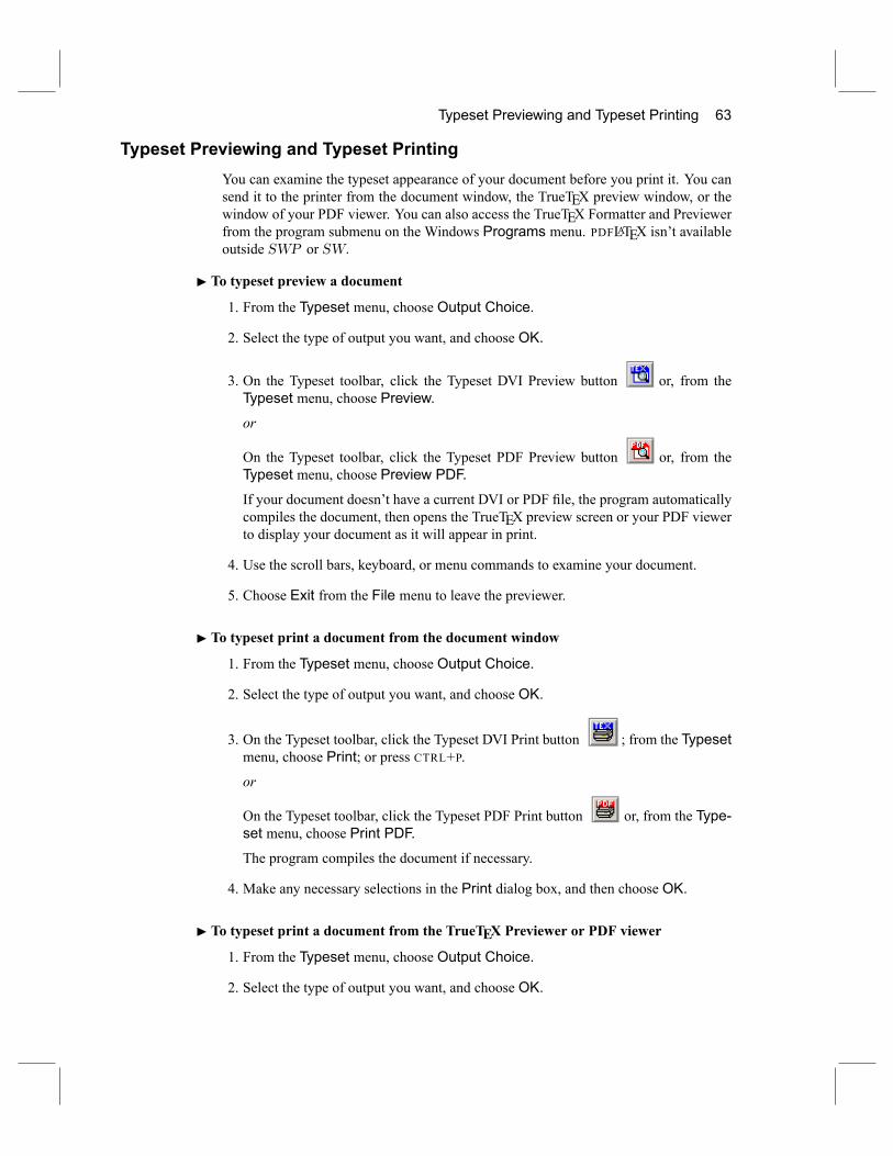
Typeset Previewing and Typeset Printing 63
Typeset Previewing and Typeset PrintingYou can examine the typeset appearance of your document before you print it. You cansend it to the printer from the document window, the TrueTEX preview window, or thewindow of your PDF viewer. You can also access the TrueTEX Formatter and Previewerfrom the program submenu on the Windows Programs menu. PDFLATEX isn't availableoutside SWP or SW.
I To typeset preview a document1. From the Typeset menu, choose Output Choice.
2. Select the type of output you want, and choose OK.
3. On the Typeset toolbar, click the Typeset DVI Preview button or, from theTypeset menu, choose Preview.
or
On the Typeset toolbar, click the Typeset PDF Preview button or, from theTypeset menu, choose Preview PDF.
If your document doesn't have a current DVI or PDF �le, the program automaticallycompiles the document, then opens the TrueTEX preview screen or your PDF viewerto display your document as it will appear in print.
4. Use the scroll bars, keyboard, or menu commands to examine your document.
5. Choose Exit from the File menu to leave the previewer.
I To typeset print a document from the document window1. From the Typeset menu, choose Output Choice.
2. Select the type of output you want, and choose OK.
3. On the Typeset toolbar, click the Typeset DVI Print button ; from the Typesetmenu, choose Print; or press CTRL+P.
or
On the Typeset toolbar, click the Typeset PDF Print button or, from the Type-set menu, choose Print PDF.
The program compiles the document if necessary.
4. Make any necessary selections in the Print dialog box, and then choose OK.
I To typeset print a document from the TrueTEX Previewer or PDF viewer1. From the Typeset menu, choose Output Choice.
2. Select the type of output you want, and choose OK.
64 Chapter 4 Typesetting Your Document
3. From the Typeset menu, choose Preview or Preview PDF.
The program compiles the document if necessary.
4. From the File menu in the TrueTEX preview window or the PDF viewer, choosePrint.
5. Select the printer and print speci�cations you want, and then choose Print.
Remember that you can use the Compile and Compile PDF commands on theTypeset menu to compile your document independently and then preview or print thetypeset document at a different time. The Compile commands are active only whenyou've saved the document and made no further changes.
I To compile a document1. From the Typeset menu, choose Output Choice.
2. Select the type of output you want, and choose OK.
3. Save the document.
4. On the Typeset toolbar, click the Typeset DVI Compile button or, from theTypeset menu, choose Compile.
or
On the Typeset toolbar, click the Typeset PDF Compile button or, from theTypeset menu, choose Compile PDF.
5. Select the options you want from the Compile or Compile PDF dialog box, andthen choose OK.
Understanding the Appearance of Typeset DocumentsWhen you typeset, the program formats your document using these speci�cations:� The typesetting speci�cations for the document shell. The speci�cations are a collec-tion of LATEX formatting instructions that govern all aspects of the typeset appearanceof your document: type face, type size, margins, page size, line spacing, location andappearance of headers and footers, paragraph layout and indention, section head-ings, page breaks, and countless other typographic details. The speci�cations arecontained in �les with extensions of .sty and .cls.
� Any speci�ed LATEX class options or LATEX packages speci�ed for the document orits shell. Class options and packages contain instructions that modify the typeset-ting speci�cations in some way. Class options are contained in �les with a .cloextension; LATEX package �les have an .sty extension.
� Any additional TEX or LATEX commands you have entered in the document itself.The typesetting speci�cations are set initially by the shell you use to create your
document. Some modi�cations to the shell and the document are possible by modifying
Creating Typeset Document Elements 65
LATEX class options, adding packages, and using commands on the Typeset menu, asdescribed in Typesetting Documents in Scienti�c WorkPlace and Scienti�c Word. Wediscourage attempts to modify the speci�cations if you aren't extremely familiar withTEX and LATEX. If the shell for your document doesn't produce the typeset results youwant, start a new document with a shell that meets your requirements more closely.
Note Don't attempt to modify the typesetting speci�cations unless you are familiarwith TEX and LATEX.
The program uses the typesetting speci�cations only when you typeset. When youproduce the document without typesetting it, the program ignores the typesetting spec-i�cations. Instead, it uses the margins, headers, footers, and page numbers speci�edin the Page Setup dialog box and the tag properties speci�ed in the style (.cst �le).Modi�cations to tag properties that you make from the Tag Appearance dialog box donot affect the typeset appearance of your document.In other words, the way you choose to produce your document determines which set
of speci�cations the program uses and, consequently, how your document appears onthe preview screen and in print.
When the document is The program formats according toProduced with LATEX or Typesetting speci�cations,PDFLATEX typesetting LATEX options and packages,
LATEX commands
Displayed in the document window Style, View settingsProduced without typesetting Style, Page setup speci�cations,
Print options
Creating Typeset Document ElementsMany document shells contain prede�ned �elds that instruct LATEX and PDFTEX to gen-erate document elements�especially those in the front matter, such as title pages andabstracts�when you typeset your document. If you don't typeset, the �elds are ignoredand the elements aren't generated.As you build your document, you can add objects that automatically create other
document elements (such as notes, citations, index entries, and cross-references to num-bered parts of the document) whenever you typeset.If you add the hyperref package to your SWP or SW document and then typeset
with PDF, the program not only creates any cross-references, page references, notes,and citations, but also converts them to hypertext links. Then, the resulting PDF �lecontains live hypertext links that you can use to jump from one part of the PDF �leto another when you view the �le with a PDF viewer. See Typesetting Documents inScienti�c WorkPlace and Scienti�c Word and the online Help for more information aboutthe hyperref package.Also, if you are very familiar with TEX and know the TEX or LATEX command for an
object or operation not available in the program, you can enter it in your document in aTEX �eld.
66 Chapter 4 Typesetting Your Document
Important Remember that you must typeset your document to generate documentelements. If you produce your document without typesetting it, the program doesn'tprocess the document with LATEX and the elements aren't generated, so the �eld or objectdoesn't appear in print.
Creating Cross-References
When you typeset your document, you can generate automatic cross-references to othernumbered objects in your document, such as equations, theorems, graphics, or sections,or to the pages on which they appear. Cross-references have two parts, a marker con-taining a key for the numbered object and the reference itself. When you typeset thedocument, the cross-reference is resolved and replaced with the number of the markedobject. The hyperref package extends cross-reference capabilities; see Creating Docu-ments with Scienti�c WorkPlace and Scienti�c Word for more information. If you don'ttypeset, cross-references and markers don't appear in print.
I To create a marker for a numbered object1. Place the insertion point where you want the marker.
2. On the Field toolbar, click the Marker button or, from the Insert menu, chooseMarker.
3. In the Key box, enter a unique key for the object, and then choose OK.
When the Markers display is turned on in the View menu, a marker looks like thisin the document window: .
4. Save the document.
Note that creating markers for graphics, numbered equations, and manual bibliogra-phy items requires a different process; see online Help for more information.
I To create a cross-reference to a numbered object1. Place the insertion point where you want the reference to appear.
2. On the Typeset Object toolbar, click the Cross Reference button or, from theInsert menu, choose Typeset Object, and then choose Cross Reference.
3. In the Print area, choose Object Counter.
4. In the Key area, enter the key of the marked object or click the arrow to the right toselect from a list of keys in the current document.
5. Choose OK.
Creating Typeset Document Elements 67
The program displays the reference on the screen in a gray box containing the word
ref and the key you entered, as in this example: .
Creating Notes
Your documents can contain references to margin notes and footnotes that appear else-where in your document. When you typeset, a cross-reference to the note is generatedand the note is formatted according to the typesetting speci�cations. If you don't typeset,footnotes and margin notes don't appear in print.
I To enter a footnote1. Place the insertion point where you want the reference to the footnote to appear.
2. On the Field toolbar, click the Note button or, from the Insert menu, chooseNote.
3. In the Type of Note box, select footnote as the type of note.
4. Enter the text of the footnote, and then choose OK.
A footnote looks like this in the document window: .
Creating Bibliographies and Citations
If the document shell supports bibliographies, you can create a bibliography list andautomatic cross-references, or citations, to items in the list. When you typeset yourdocument, the citation is generated and formatted correctly, according to the typesettingspeci�cations for the shell.You can create bibliographies in two ways. If your bibliography is complex, you
can create an automatic bibliography using BIBTEX, a public domain program createdby Oren Patashnik. BIBTEX generates and formats the bibliography list automatically byextracting references from a database using the citations you insert into your document.Because you don't have to create the bibliography list yourself, a BIBTEX bibliographyis convenient if you have a long list of references that you plan to use in other articlesor books. The creation and use of BIBTEX bibliographies is somewhat complex. Pleaserefer to the online Help for detailed instructions.If your bibliography is a simple one, you can create it manually. A manual bibliog-
raphy, which works just like a series of cross-references, is convenient when your list ofreferences is short and you don't plan to use those references in other articles or books.You must format entries in a manual bibliography yourself.
I To specify a manual bibliography1. From the Typeset menu, choose Bibliography Choice.
2. SelectManual Entry and choose OK.
68 Chapter 4 Typesetting Your Document
I To create a list of bibliography items1. Move the insertion point to the end of the line that is to precede the bibliography,and press ENTER.
2. Apply the Bibliography Item tag.
3. In the Bibliography Item Properties dialog box, enter a unique key for the item andchoose OK.
4. Type the bibliographic information for the item.
5. If you want to create another bibliographic item, press ENTER and repeat steps 3�4.
6. When you have completed all the entries, press ENTER and then click to leavethe list.
I To create a citation for an item in a manual bibliography1. Place the insertion point where you want the citation to appear.
2. On the Typeset Object toolbar, click the Citation button or, from the Insertmenu, choose Typeset Object, and then choose Citation.
3. In the Citation dialog box, enter the key for the bibliography item you want to cite,and then choose OK.
In the document window, you see the citation in a small gray box containing the keyfor the bibliography item, like this: . When you typeset the document, thenumber of the item in the bibliography list replaces the key.
Obtaining More Information About Typesetting
A detailed discussion of LATEX typesetting is beyond the scope of this booklet. How-ever, you can �nd much more information about typesetting with SWP and SW in thefollowing sources:� The online Help.� Creating Documents with Scienti�c WorkPlace and Scienti�c Word.� Typesetting Documents in Scienti�c WorkPlace and Scienti�c Word.You can �nd more information about LATEX in these books:� LATEX, A Document Preparation System by Leslie Lamport.� The LATEX Companion byMichel Goossens, FrankMittelbach, and Alexander Samarin.� A Guide to LATEX: Document Preparation for Beginners and Advanced Users byHelmut Kopka and Patrick W. Daly.
Also, you can �nd information about TEX in The TEXbook by Donald E. Knuth.
5 Getting the Most from YourSoftware
SWP, SW, and SNB are straightforward and easy to use, especially if you take ad-vantage of the many resources available to you. The program is supplied with docu-mentation including a Help system and tutorial materials that can help you learn howto create documents and enter mathematics. If you have an Internet connection, ad-ditional documentation�in particular, the Help system for SV�is available from theMacKichan Software website. Additionally, three manuals provide program details:� Creating Documents with Scienti�c WorkPlace and Scienti�c Word provides infor-mation about entering and editing text and mathematics; formatting documents;structuring documents for typesetting and for use online; maintaining �les; and cus-tomizing your installation. Much of the information in the manual is applicable toSNB.
� Doing Mathematics with Scienti�c WorkPlace and Scienti�c Notebook explains howto use the built-in computer algebra system to do mathematics without dealing di-rectly with the syntax of the computer algebra system. Along with examples andexercises, the manual provides basic procedures for using the system to computeand plot and to solve problems in analytic geometry, calculus, linear algebra, vectoranalysis, differential equations, statistics, and applied modern algebra.
� Typesetting Documents in Scienti�c WorkPlace and Scienti�c Word provides answersto common questions about LATEX typesetting in SWP and SW. It helps you choosedocument shells appropriately and explains when and how to tailor document shellsfrom within the program so that the documents you create meet your typesettingneeds more precisely.Accompanying this version of the program is another volume, A Gallery of Docu-
ment Shells for Scienti�c WorkPlace and Scienti�c Word, available on your program CD.A Gallery of Document Shells explains the key characteristics of the shells provided withthe program. It contains brief discussions and illustrations of typeset documents createdwith each shell (except those created with SNB, which are not intended for typesetting).If you can't �nd the information you need in one of these resources, technical support
is available. We regularly make additional information available on our unmoderateddiscussion forum and email list. We also have an electronic newsletter that you canrequest on our website or when you register your program.
70 Chapter 5 Getting the Most from Your Software
Using Online HelpThe program includes an extensive Help system available online or from your CD-ROM.While you're working, you can get information quickly from the online Help feature.You can search Help to �nd basic and advanced information about commands and oper-ations, including instructions for using the built-in computational engine to perform nu-meric, symbolic, and graphic computations. If you save copies of the Help documents inSWP or SNB, you can interact with the mathematics they contain, experimenting withor reworking the included examples. In addition, two programs�the Style Editor andthe Document Manager�have their own online Help.
I To use the Help system� From the Help menu, choose the command you need:
Choose ToContents See a list of online informationSearch... Find a Help topicIndex Access the online index to General Information,
Computing Techniques, or the Reference LibraryMacKichan Software Open the link to the MacKichan Software, Inc.Website websiteRegister... Register your software and obtain a licenseSystem Features... See a list of available features; change the serial
number for your installationLicense Information Obtain information about registering your systemAbout... Obtain information about your installation
Also, we urge you to explore the supplemental technical documents supplied withthe program. You can open, view, and print the documents. In particular, we suggestyou read the following documents:� The document 50techref.tex in the Helpngeneral directory, which containstechnical information on the features in Version 5.
� The documents in the Play directory, which demonstrate the use of computation inSWP and SNB.
� The documents in the SNSamples directory, which are examples of online docu-ments created with the program.
� The documents in the SWSamples directory, which include examples of documentsintended for typesetting in SWP and SW.

Obtaining Additional Information 71
Obtaining Technical SupportIf you can't �nd the answer to your questions in the manuals or the online Help, you canobtain technical support from our website at
http://www.mackichan.com/techtalk/knowledgebase.html
or from our Web-based Technical Support forum at
http://www.mackichan.com/techtalk/UserForums.htm
You can also contact our Technical Support staff by email, telephone, or fax. We urgeyou to submit questions by email whenever possible in case our technical staff needs toobtain your �le to diagnose and solve the problem.When you contact us by email or fax, please provide complete information about
the problem you're trying to solve. We must be able to reproduce the problem exactlyfrom your instructions. When you contact us by telephone, you should be sitting at yourcomputer with the program running.Please provide the following information any time you contact Technical Support:
� The MacKichan Software product you have installed.� The version and build numbers of your installation (see Help / About).� The serial number of your installation (see Help / System Features).� The version of the Windows system you're using.� The type of hardware you're using, including network hardware.� A description of what happened and what you were doing when the problem oc-curred.
� The exact wording of any messages that appeared on your computer screen.
I To contact technical support� Contact Technical Support by email, fax, or telephone between 8 AM and 5 PM Pa-ci�c Time:
Internet email address: [email protected]: 360-394-6039
Telephone: 360-394-6033Toll-free telephone: 877-SCI-WORD (877-724-9673) or
877-SCI-NOTE (877-724-6683)
Obtaining Additional InformationYou can learn more about the program on our website, which we update regularly toprovide the latest technical information about the software. The site also houses links toother TEX and LATEX resources. We maintain an unmoderated discussion forum and anunmoderated email list so our users can share information, discuss common problems,and contribute technical tips and solutions. You can link to these valuable resourcesfrom our home page at
http://www.mackichan.com
72 Chapter 5 Getting the Most from Your Software
Learning to Use the Program
You can learn a great deal about the program just by working with it. Start by openingthe program, typing a few sentences, entering some mathematics, and then previewingand printing your document, as described in Chapter 1 �Tools for Scienti�c Creativity.�We also urge you to work through the tutorial exercises, available from online Help.
The exercises guide you step-by-step as you create several increasingly complex doc-uments and learn how to enter a variety of mathematical expressions, compute whileworking in your document, and print with and without typesetting.
I To open the tutorial exercises1. From the Help menu, choose Contents.
2. Choose Learn the Basics.
3. Choose the exercise you want:� �Before You Start� provides information about the notation, terminology, andinstructions used in the exercises.
� �Creating a Simple Document� provides instructions for creating a basic docu-ment.
� �Printing and Typesetting� explains several ways to produce your document.� �Creating an Advanced Document� gives instructions for creating a somewhatmore complex document in SWP or SW. The exercise, which takes about 90minutes to complete, focuses on document structuring, guiding you step-by-stepthrough the unique procedures for creating titles, headings, and theorem state-ments. Because the document you create contains equations, the exercise alsoillustrates the straightforward entry and editing of mathematics.
� �Creating Mathematics� presents a series of mathematical examples. The exer-cises give step-by-step instructions for entering a variety of mathematical expres-sions using the mouse and the keyboard.
� �Sharing Your Work� presents information about creating documents for useacross platforms, installations, and systems; on a network; or on the Web.
� �Performing Computations� presents a series of mathematical computation ex-ercises. The step-by-step instructions guide you through basic computationalprocedures for SWP and SNB.
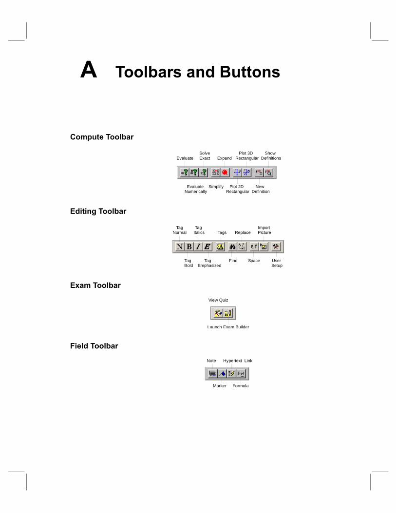
A Toolbars and Buttons
Compute Toolbar
Solve Plot 3D ShowEvaluate Exact Expand Rectangular Definitions
Evaluate Simplify Plot 2D NewNumerically Rectangular Definition
Editing Toolbar
Tag Tag ImportNormal Italics Tags Replace Picture
Tag Tag Find Space UserBold Emphasized Setup
Exam Toolbar
View Quiz
Launch Exam Builder
Field Toolbar
Note Hypertext Link
Marker Formula
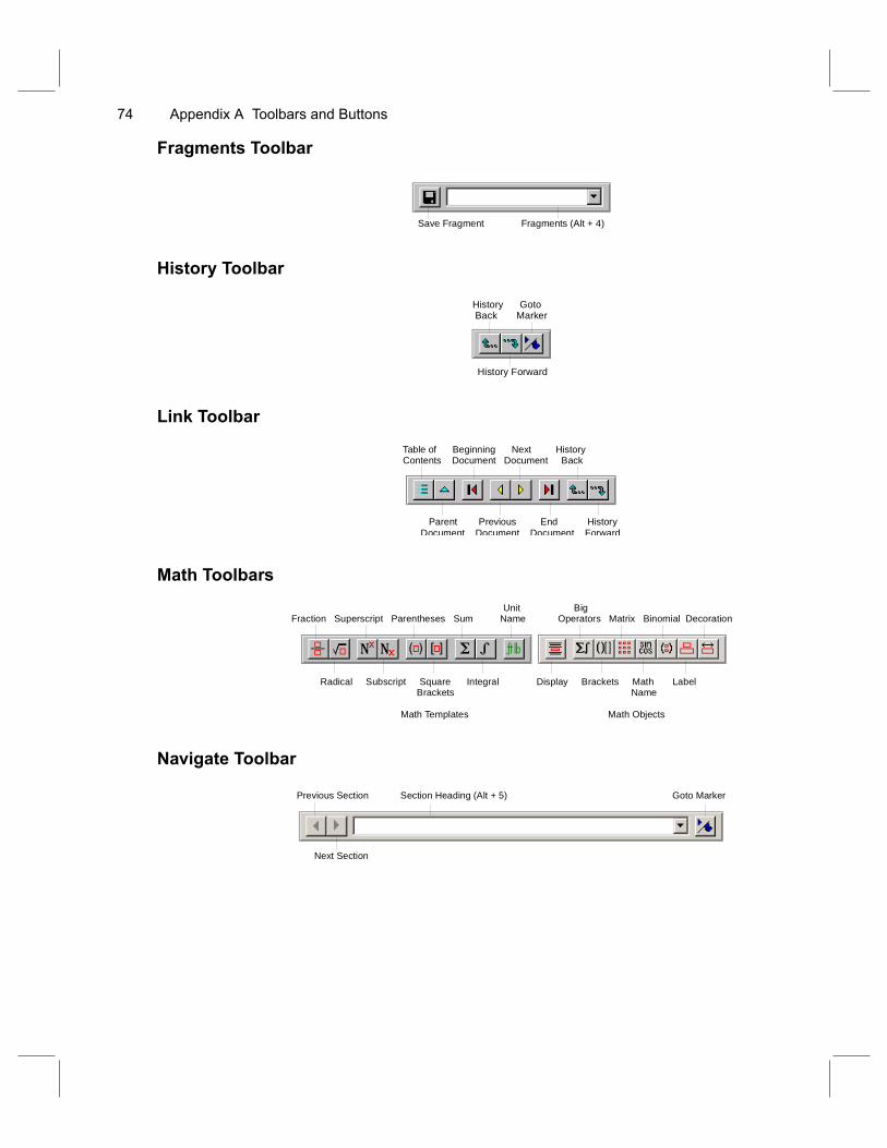
74 Appendix A Toolbars and Buttons
Fragments Toolbar
Fragments (Alt + 4)Save Fragment
History Toolbar
History GotoBack Marker
History Forward
Link Toolbar
Table of Beginning Next HistoryContents Document Document Back
Parent Previous End HistoryDocument Document Document Forward
Math Toolbars
Unit BigFraction Superscript Parentheses Sum Name Operators Matrix Binomial Decoration
Radical Subscript Square Integral Display Brackets Math LabelBrackets Name
Math Templates Math Objects
Navigate Toolbar
Previous Section Section Heading (Alt + 5) Goto Marker
Next Section
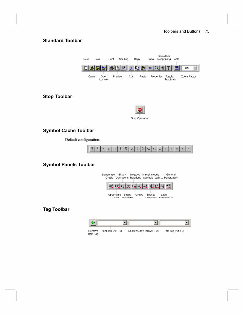
Toolbars and Buttons 75
Standard Toolbar
Show/HideNew Save Print Spelling Copy Undo Nonprinting Table
Open Open Preview Cut Paste Properties Toggle Zoom FactorLocation Text/Math
Stop Toolbar
Stop Operation
Symbol Cache Toolbar
Default con�guration:
Symbol Panels Toolbar
Lowercase Binary Negated Miscellaneous GeneralGreek Operations Relations Symbols Latin1 Punctuation
Uppercase Binary Arrows Special LatinGreek Relations Delimiters ExtendedA
Tag Toolbar
Remove Item Tag (Alt + 1) Section/Body Tag (Alt + 2) Text Tag (Alt + 3)Item Tag
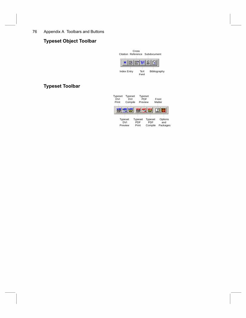
76 Appendix A Toolbars and Buttons
Typeset Object Toolbar
CrossCitation Reference Subdocument
Index Entry TeX BibliographyField
Typeset Toolbar
Typeset Typeset TypesetDVI DVI PDF FrontPrint Compile Preview Matter
Typeset Typeset Typeset OptionsDVI PDF PDF and
Preview Print Compile Packages
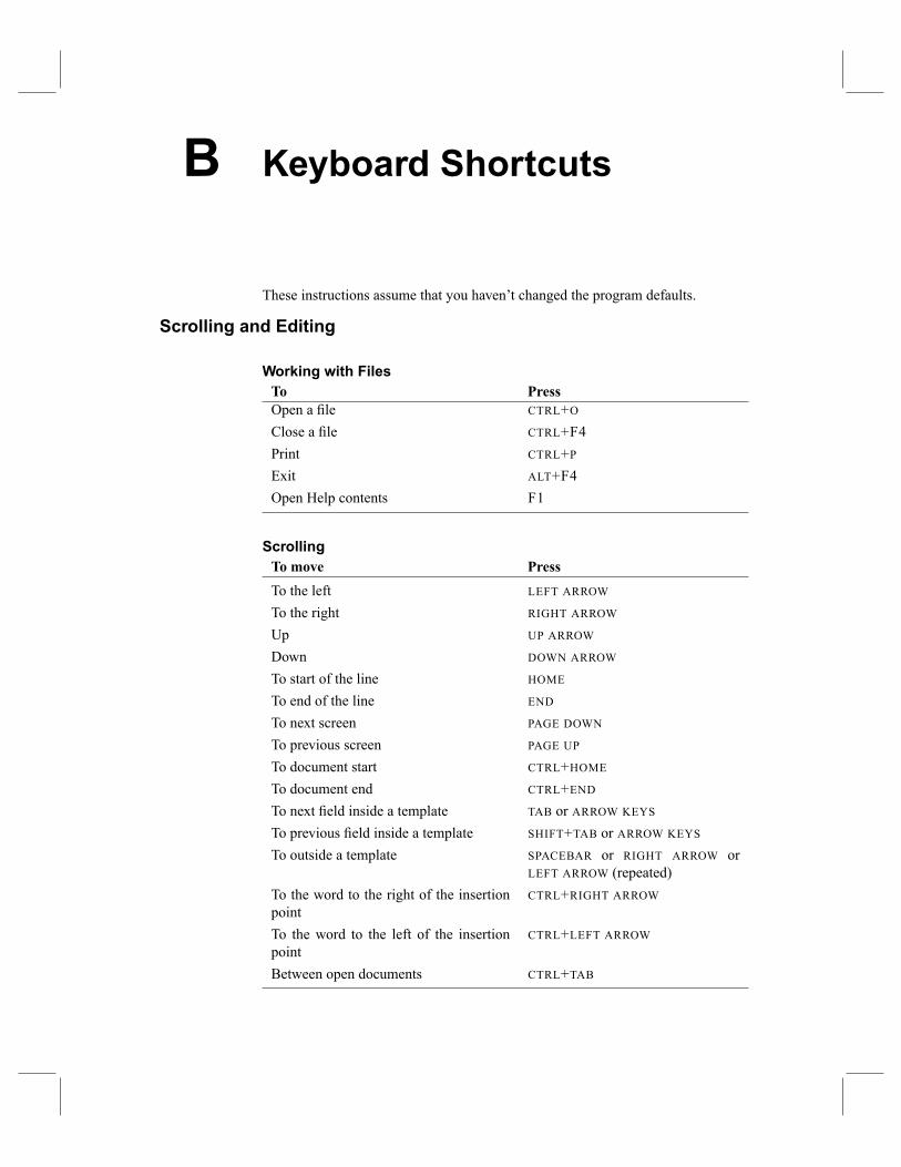
B Keyboard Shortcuts
These instructions assume that you haven't changed the program defaults.
Scrolling and Editing
Working with FilesTo PressOpen a �le CTRL+OClose a �le CTRL+F4Print CTRL+PExit ALT+F4Open Help contents F1
ScrollingTo move PressTo the left LEFT ARROW
To the right RIGHT ARROW
Up UP ARROW
Down DOWN ARROW
To start of the line HOME
To end of the line END
To next screen PAGE DOWN
To previous screen PAGE UP
To document start CTRL+HOMETo document end CTRL+ENDTo next �eld inside a template TAB or ARROW KEYS
To previous �eld inside a template SHIFT+TAB or ARROW KEYS
To outside a template SPACEBAR or RIGHT ARROW orLEFT ARROW (repeated)
To the word to the right of the insertionpoint
CTRL+RIGHT ARROW
To the word to the left of the insertionpoint
CTRL+LEFT ARROW
Between open documents CTRL+TAB
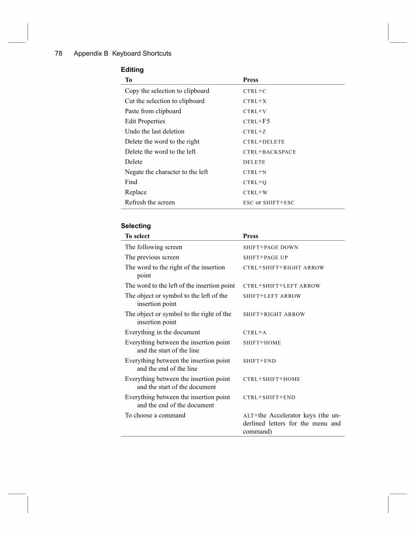
78 Appendix B Keyboard Shortcuts
EditingTo PressCopy the selection to clipboard CTRL+CCut the selection to clipboard CTRL+XPaste from clipboard CTRL+VEdit Properties CTRL+F5Undo the last deletion CTRL+ZDelete the word to the right CTRL+DELETEDelete the word to the left CTRL+BACKSPACEDelete DELETE
Negate the character to the left CTRL+NFind CTRL+QReplace CTRL+WRefresh the screen ESC or SHIFT+ESC
SelectingTo select PressThe following screen SHIFT+PAGE DOWNThe previous screen SHIFT+PAGE UPThe word to the right of the insertion
pointCTRL+SHIFT+RIGHT ARROW
The word to the left of the insertion point CTRL+SHIFT+LEFT ARROWThe object or symbol to the left of the
insertion pointSHIFT+LEFT ARROW
The object or symbol to the right of theinsertion point
SHIFT+RIGHT ARROW
Everything in the document CTRL+AEverything between the insertion point
and the start of the lineSHIFT+HOME
Everything between the insertion pointand the end of the line
SHIFT+END
Everything between the insertion pointand the start of the document
CTRL+SHIFT+HOME
Everything between the insertion pointand the end of the document
CTRL+SHIFT+END
To choose a command ALT+the Accelerator keys (the un-derlined letters for the menu andcommand)
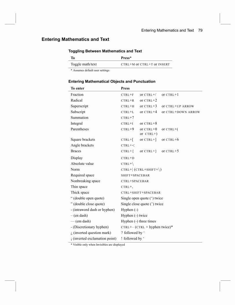
Entering Mathematics and Text 79
Entering Mathematics and Text
Toggling Between Mathematics and Text
To Press*Toggle math/text CTRL+M or CTRL+T or INSERT* Assumes default user settings
Entering Mathematical Objects and Punctuation
To enter PressFraction CTRL+F or CTRL+/ or CTRL+1Radical CTRL+R or CTRL+2Superscript CTRL+H or CTRL+3 or CTRL+UP ARROWSubscript CTRL+L or CTRL+4 or CTRL+DOWN ARROWSummation CTRL+7Integral CTRL+I or CTRL+8Parentheses CTRL+9 or CTRL+0 or CTRL+(
or CTRL+)Square brackets CTRL+[ or CTRL+] or CTRL+6Angle brackets CTRL+<Braces CTRL+{ or CTRL+} or CTRL+5
Display CTRL+DAbsolute value CTRL+nNorm CTRL+j (CTRL+SHIFT+n)Required space SHIFT+SPACEBARNonbreaking space CTRL+SPACEBARThin space CTRL+,Thick space CTRL+SHIFT+SPACEBAR� (double open quote) Single open quote (`) twice� (double close quote) Single close quote (') twice- (intraword dash or hyphen) Hyphen (-)� (en dash) Hyphen (-) twice� (em dash) Hyphen (-) three times- (Discretionary hyphen) CTRL+� (CTRL + hyphen twice)*¿ (inverted question mark) ? followed by `¡ (inverted exclamation point) ! followed by `* Visible only when Invisibles are displayed
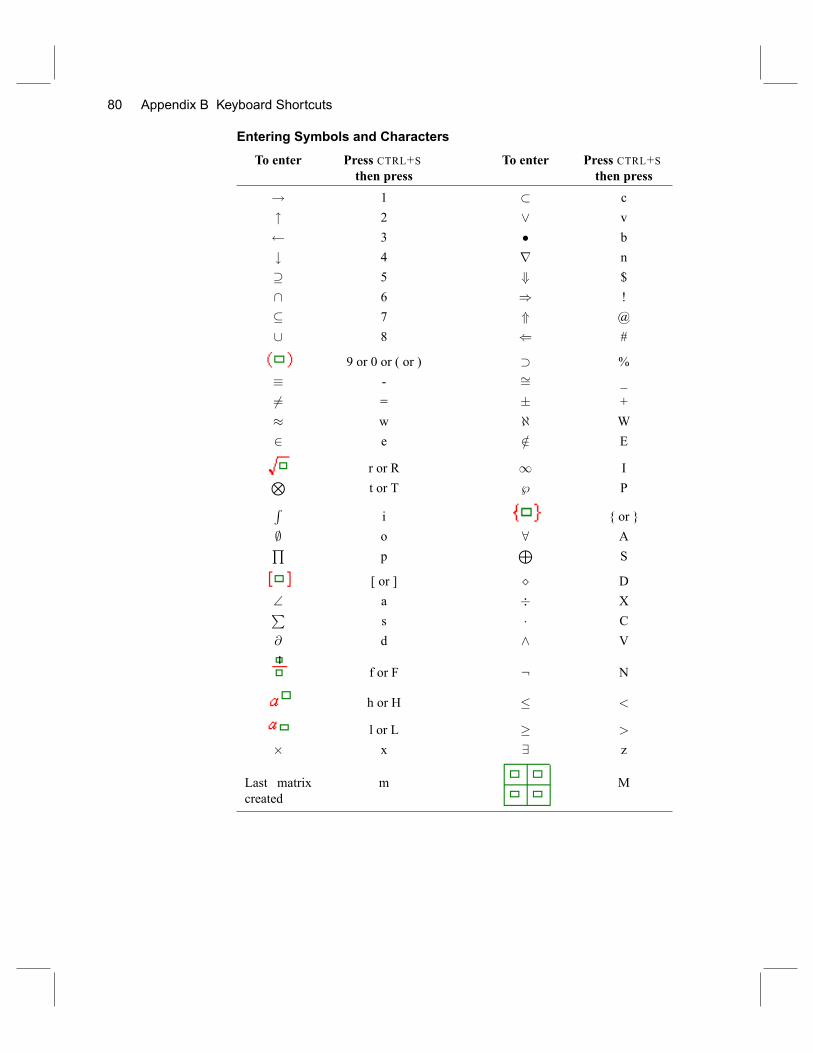
80 Appendix B Keyboard Shortcuts
Entering Symbols and Characters
To enter Press CTRL+S To enter Press CTRL+Sthen press then press
! 1 � c" 2 _ v 3 � b# 4 r n� 5 + $\ 6 ) !� 7 * @[ 8 ( #
9 or 0 or ( or ) � %� - �= _6= = � +� w @ W2 e =2 E
r or R 1 INt or T } PRi { or }
; o 8 AQp
LS
[ or ] � D\ a � XP
s � C@ d ^ V
f or F : N
h or H � <
l or L � >
� x 9 z
Last matrixcreated
m M
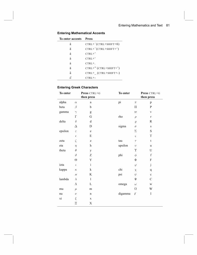
Entering Mathematics and Text 81
Entering Mathematical Accents
To enter accents Pressâ CTRL+^(CTRL+SHIFT+6)ã CTRL+~(CTRL+SHIFT+`)á CTRL+'à CTRL+`�a CTRL+.ä CTRL+� (CTRL+SHIFT+')a CTRL+_ (CTRL+SHIFT+-)~a CTRL+-
Entering Greek Characters
To enter Press CTRL+G To enter Press CTRL+Gthen press then press
alpha � a pi � pbeta � b � Pgamma g $ v
� G rho � rdelta � d % R
� D sigma � sepsilon " e � S
� E & Tzeta � z tau � teta � h upsilon � utheta � y � U
# Z phi � f� Y � F
iota � i ' jkappa � k chi � q
{ K psi clambda � l C
� L omega ! wmu � m Wnu � n digamma z Ixi � x
� X
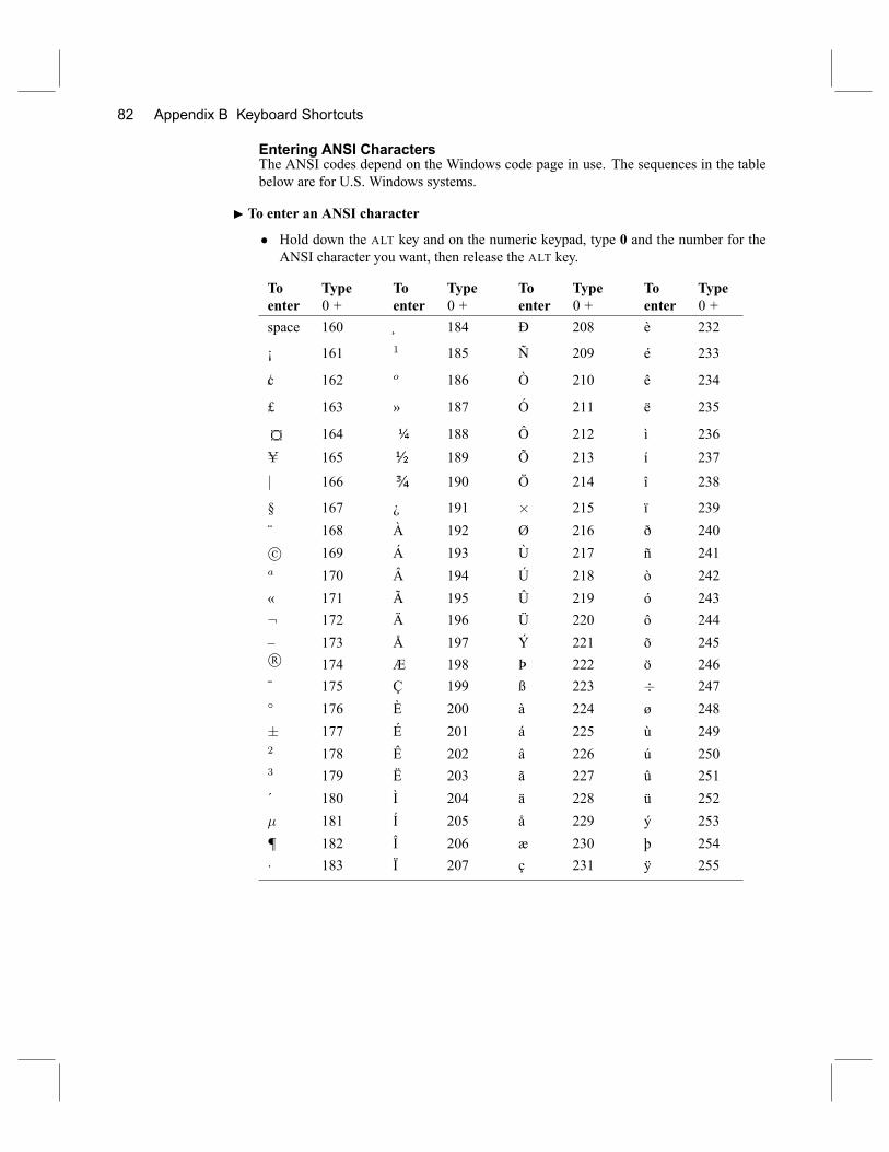
82 Appendix B Keyboard Shortcuts
Entering ANSI CharactersThe ANSI codes depend on the Windows code page in use. The sequences in the tablebelow are for U.S. Windows systems.
I To enter an ANSI character� Hold down the ALT key and on the numeric keypad, type 0 and the number for theANSI character you want, then release the ALT key.
Toenter
Type0 +
Toenter
Type0 +
Toenter
Type0 +
Toenter
Type0 +
space 160 ¸ 184 Ð 208 è 232
¡ 161 1 185 Ñ 209 é 233
c/ 162 o 186 Ò 210 ê 234
£ 163 » 187 Ó 211 ë 235
164 188 Ô 212 ì 236U 165 189 Õ 213 í 237
j 166 190 Ö 214 î 238
§ 167 ¿ 191 � 215 ï 239¨ 168 À 192 Ø 216 ð 240c 169 Á 193 Ù 217 ñ 241a 170 Â 194 Ú 218 ò 242« 171 Ã 195 Û 219 ó 243: 172 Ä 196 Ü 220 ô 244� 173 Å 197 Ý 221 õ 245R 174 Æ 198 Þ 222 ö 246¯ 175 Ç 199 ß 223 � 247� 176 È 200 à 224 ø 248� 177 É 201 á 225 ù 2492 178 Ê 202 â 226 ú 2503 179 Ë 203 ã 227 û 251´ 180 Ì 204 ä 228 ü 252� 181 Í 205 å 229 ý 253{ 182 Î 206 æ 230 þ 254� 183 Ï 207 ç 231 ÿ 255
Index
accents, 81adding tags, 24additional informationdocumentation, 69technical support, 71typesetting, 68
appearance of documentsabout, 4modifying the style, 22on screen, 20, 62style, 20text format, 21typesetting speci�cations,64
with typesetting, 20, 62, 64without typesetting, 20
bibliographies, 67BIBTEX, 67body math, 20body tags, 21body text, 22bold, 22browsing the Internet, 11, 29buttons, toolbar, 73
centering, 21characters and symbolsaccents, 81ANSI characters, 82entering, 15Greek characters, 81mathematics, 80properties, 16symbol panels, 15, 35
checking equalities, 46citations, 67class options, 64cloning tags, 24closing documents, 11combining terms, 43compiling documents, 64computationschecking equalities, 46combining terms, 43computing in place, 55
computing statistics, 58computing with units ofmeasure, 59
evaluating, 40evaluating numerically, 40expanding expressions, 44factoring expressions, 42introduction, 9matrix operations, 56plotting, 51simplifying expressions, 45solving differential equa-tions, 57
solving expressions, 47stopping, 39working with polynomials,49
Compute menu commandsCheck Equality, 46Combine, 43Evaluate, 40Evaluate Numerically, 40Expand, 44Factor, 42Matrix, 56Plot 2D, 51Plot 3D, 53Polynomials, 49Simplify, 45Solve Exact, 47Solve Numeric, 47Solve ODE, 57Statistics, 58
Compute toolbar, 39, 73computing in place, 55conversion with units, 59copy, 16course materials, creating, 60cross-referencescreating, 66in PDF �les, 65
.cst �le, 20cursor, 13customer support, 71customizing the program, 33cut, 16
default settingsfunction keys, 36program defaults, 37
device independent (DVI)�les, 62
differential equations, 57displayed mathematics, 19displaying toolbars, 14docking toolbars, 33document appearanceabout, 4modifying the style, 22on screen, 20, 62style, 20text format, 21typesetting speci�cations,64
with typesetting, 20, 62, 64without typesetting, 20
Document Manager, 31document windows, 35documentationfor LATEX, 68online Help, 70program, 68, 69
documentsclosing, 11compiling, 64document elements, 65exporting, 28, 30formatting, 20new, 14on the Web, 29opening, 14previewing and printing,28, 63
saving, 27shells, 14, 64style, 20, 22typesetting, 61view, 35window, 33
drag and drop, 16DVI �lescompiling, 62previewing and printing, 63
84 Index
editingmathematics, 20shortcuts, 78text, 16
Editing toolbar, 73emphasizing text, 22entering mathematics, 16entering text, 15evaluating expressions, 39Exam Builder, 60Exam toolbar, 73exerciseschecking equalities, 46combining terms, 43computing in place, 55computing statistics, 58computing with units ofmeasure, 59
creating exams, 60evaluating, 40evaluating numerically, 40expanding expressions, 44factoring, 42matrix operations, 56plotting, 51simplifying expressions, 45solving differential equa-tions, 57
solving expressions, 47working with polynomials,49
expanding expressions, 44exporting a documentHTML �les, 30portable LATEX �les, 27RTF �les, 28
factoring expressions, 42Field toolbar, 65, 73�elds, 65�le formatsDVI �les, 63PDF �les, 64RTF �les, 28.tex �les, 27
�lesDVI �les, 63exporting, 28, 30formatting, 20HTML �les, 30opening, 14
PDF �les, 29, 63portable LATEX �les, 27previewing and printing, 28RTF �les, 28saving, 27typesetting, 61
�ltersHTML �lter, 30portable LATEX �lter, 27
�oating a toolbar, 33fontsproperties, 24text tags, 22
footnotes, 67foreign characters, 15formattingabout, 4modifying the style, 23on screen, 20style, 20text format, 21typesetting speci�cations,20, 64
with typesetting, 20, 62, 64without typesetting, 20
fractions, 17fragments, 19Fragments toolbar, 19, 74function key assignments, 21,
36
Greek characters, 81
hardware requirements, 5headings, 21help, 70Help menu commands, 70History toolbar, 74HTML �les, 30hyperref package, 65hypertext linkscreating, 25from cross-references, 65hyperref package, 65in PDF �les, 29jumping with, 26
in-line mathematics, 19inherited tag properties, 23insertion point, 13installing the program
installation requirements, 5on personal computers, 5program license, 5
Internet, 11, 29italics, 22item tags, 22
jumping with hypertext, 26
keyboard shortcuts, 77keys, creating, 26, 66
LATEXclass options, 64compiling, 64described, 62document appearance, 64DVI �les, 62packages, 64PDF �les, 62portable LATEX �les, 27resources, 68
lead-in object, 24learning the program, 72leaving the program, 11licensing the program, 5limits, 19Link toolbar, 74linkscreating, 25from cross-references, 65hyperref package, 65in PDF �les, 29jumping with, 26to the Internet, 31
listscreating, 22lead-in object, 24
logical design, 3
MacKichan, contacting, 71magni�cation, 36margin notes, 67margins, 25markers, creating, 26, 66Math toolbars, 17, 74Math/Text toggle, 8, 15, 16mathematical characters and
symbolsaccents, 81ANSI characters, 82
Index 85
entering, 15Greek characters, 81mathematics, 80properties, 16symbol panels, 15, 35
mathematical objectsentering, 17, 39, 79templates, 17
mathematical operators, 18mathematicsbody math paragraphs, 20computations, 39computing in place, 55different from text, 16displayed, 19editing, 20entering, 16, 39in-line, 19Math/Text toggle, 16screen appearance, 16shortcuts, 79stopping computations, 39
matrixcomputations, 56entering, 18
Microsoft Windows, 5modifying page setup, 25modifying the style, 23
Navigate toolbar, 74new document, 7non-English characters, 15notes, 67
online documentation, 69, 70online documents, 29online Help, 70Open Location, 11, 31opening documents, 14opening the program, 5opening websites, 11, 29operators, mathematical, 18
packages, 64page formatheaders and footers, 25margins, 25modifying the style, 23typesetting speci�cations,22, 62
page numbering, 25
paragraphsformat, 24text and mathematics in, 15
parentheses, 18paste, 16PDF �lescreating, 29previewing and printing, 63typesetting, 62
PDFLATEX, 62PDFTEX, 62personal computer installa-
tions, 5physical units, 59plottingmathematics, 10, 39, 51plot captions, 24
polynomials, 49popup lists, 21Portable Document Format
(PDF), 62portable LATEX �les, 27previewing documentswith typesetting, 63without typesetting, 28
print styledocument appearance, 20modifying, 22
printing documentsfrom preview screen, 29previewing before, 63with typesetting, 63without typesetting, 10, 29
product features, 1, 2programleaving, 11opening, 7
program defaults, 37program installationobtaining a license, 5personal computer, 5requirements, 5
program resourcesonline Help, 70technical support, 71website, 71
program window, 7, 13propertiesContext menu, 16editing, 16, 20
tags, 21, 23
radicals, 40registering the program, 5Remove Item Tag button, 22Rich Text Format (RTF) �les,
28
saving documents, 11, 27screen appearance, 9, 20, 21,
36scrolling, 77section headings, 21section tags, 21selecting mathematics and
text, 78settingsfunction keys, 36program defaults, 37
shell documents, 14, 64shortcuts, 77simplifying expressions, 45software requirements, 5solving expressions, 47speci�cations, typesetting, 20,
64spell checks, 16Standard toolbar, 13, 75starting mathematics, 16starting the program, 5statistics, 58Stop toolbar, 39, 75stopping a computation, 39styledocument appearance, 20modifying, 23
subscripts and superscripts, 18Symbol Cache toolbar, 17, 35,
75symbol panelscustomizing, 34entering symbols from, 15
Symbol Panels toolbar, 15, 75symbols and charactersaccents, 81ANSI characters, 82entering, 15Greek characters, 81mathematics, 80properties, 16symbol panels, 15, 35
86 Index
tables, 15tag properties, 4, 23Tag toolbar, 21, 75tagged text, 21tagsadding, 24formatting with, 21function key assignments,36
properties, 4technical support, 71templates, 17TEXentering mathematics, 17�elds, 65LATEX, 62PDFLATEX, 62pdfTEX, 62resources, 68TrueTEX, 62typesetting, 61, 64
.tex �leson the web, 31saving, 27
textdifferent from mathematics,16
editing, 16entering, 15formatting, 21screen appearance, 9, 21
text tags, 22toll-free number, 71toolbarsbuttons, 73
Compute toolbar, 39, 73customizing, 33displaying, 8, 14docking, 33Editing toolbar, 73Exam toolbar, 73Field toolbar, 65, 73�oating, 33Fragments toolbar, 19, 74History toolbar, 74illustrated, 73�75Link toolbar, 74Math toolbars, 17, 74Navigate toolbar, 74Standard toolbar, 13, 61, 75Stop toolbar, 39, 75Symbol Cache toolbar, 17,35, 75
Symbol Panels toolbar, 15,75
Tag toolbar, 21, 75Typeset Object toolbar, 65,76
Typeset toolbar, 61, 76viewing, 8, 14
tooltips, 13troubleshooting, 71TrueTEX, 62tutorial exercises, 72Typeset Object toolbar, 65, 76Typeset toolbar, 29, 61, 76typesettingabout, 61appearance, 65bibliographies, 67
citations, 68class options, 64cross-references, 66DVI �les, 62footnotes, 67LATEX packages, 64PDF �les, 29previewing and printing, 63process, 62resources, 68speci�cations, 20, 64
undo, 16Uniform Resource Locator
(URL), 71unit names, 59units of measure, 59unwrapping �les, 33URL, 71
View menu commands, 36viewing toolbars, 14visual design, 3
website for MacKichan, 71windowscustomizing, 35document window, 33program window, 7, 13
Windows, Microsoft, 5World Wide Web, 11, 29wrapping �les, 32
zoom factor, 36


![Skaffold - storage.googleapis.com · [getting-started getting-started] Hello world! [getting-started getting-started] Hello world! [getting-started getting-started] Hello world! 5](https://img.pdfslide.net/doc/110x75/5ec939f2a76a033f091c5ac7/skaffold-getting-started-getting-started-hello-world-getting-started-getting-started.jpg)