Embed Size (px)
Citation preview
9042 2021
April 2021
Does Size Matter? Evidence from Municipality Break-Ups Gissur Ó Erlingsson, Jonas Klarin, Eva Mörk
Impressum:
CESifo Working Papers ISSN 2364-1428 (electronic version) Publisher and distributor: Munich Society for the Promotion of Economic Research - CESifo GmbH The international platform of Ludwigs-Maximilians University’s Center for Economic Studies and the ifo Institute Poschingerstr. 5, 81679 Munich, Germany Telephone +49 (0)89 2180-2740, Telefax +49 (0)89 2180-17845, email [email protected] Editor: Clemens Fuest https://www.cesifo.org/en/wp An electronic version of the paper may be downloaded · from the SSRN website: www.SSRN.com · from the RePEc website: www.RePEc.org · from the CESifo website: https://www.cesifo.org/en/wp
CESifo Working Paper No. 9042
Does Size Matter? Evidence from Municipality Break-Ups
Abstract Municipal break-ups are an understudied phenomenon despite the fact that such territorial reforms regularly take place across the globe. This paper estimates how seven voluntary splits of Swedish municipalities affected municipal current costs. To predict what would have happened had the break-ups not taken place, we apply the matrix completion method with nuclear norm minimization. Our results do not support the standard view, that smaller municipalities imply higher per capita costs. Instead, we find an intriguing heterogeneity: costs increase in some municipalities, are unaffected in others and decrease elsewhere. The findings point to the complex nature of territorial reforms, the difficulty in drawing general conclusions of such, and hence, the perils of expecting them to have uniform outcomes. JEL-Codes: H720, R120, R500. Keywords: territorial reforms, municipalities, matrix completion.
Gissur Ó Erlingsson Centre for Local Government Studies
Linköping University / Sweden [email protected]
Jonas Klarin Department of Economics & UCFS
Uppsala University / Sweden [email protected]
Eva Mörk
Department of Economics, UCFS, UCLS & Urban Lab Uppsala University / Sweden
[email protected] April 22, 2021 We are grateful for comments and suggestions from Traviss Cassidy, Che-Yuan Liang, Mattias Nordin, Luca Repetto, John Östh, Jonas Öman, participants at the 76th Annual Congress of the IIPF, as well as from seminar participants at CKS in Linköping, and the Urban Lab and the Department of Economics in Uppsala. We thank Jason Poulos, Che-Yuan Liang and Anil Kumar for generously sharing their R-codes. We also thank Jacob Pelgander at SCB Örebro for assisting us in the search for historical data of municipal finances. Klarin thanks The Jan Wallander and Tom Hedelius Foundation for financial support.
1 Introduction
Since the mid-1990s, amalgamations of municipalities have been placed high on polit-
ical agendas across the globe (Bouckaert and Kuhlman, 2016; Fox and Gurley, 2006).
The underlying rationale is almost always economic. By merging smaller units into
larger, policy-makers hope to reap the benefits of economies of scale and form finan-
cially more viable municipalities. However, parallel with this general trend, local
forces in, above all, several Central and Eastern European countries – but also in
Sweden and Spain – have pushed in the opposite direction, which have resulted in a
number of municipality break-ups. In light of current debates on the appropriate size
of local governments, this paper asks how municipal costs are affected by municipal
splits, and to what extent it is reasonable to expect homogeneous effects of territorial
reforms.
By now, there exists an extensive empirical literature studying the economic con-
sequences of municipal amalgamations.1 While a few studies have found decreasing
costs as a consequence of amalgamations – most notably Reingewertz (2012) on Is-
raeli data – the general conclusion is nevertheless that, although administrative costs
tend to decrease, total per capita costs remain largely unchanged (see, for instance,
Tavares (2018) and Gendzwill et al. (2020) for literature reviews). However, whereas
occasional descriptive case studies or purely theoretical papers exist (de Souza et al.,
2015; Dollery et al., 2011; Erlingsson, 2005), empirical studies aiming at estimating
causal effects of municipal splits remain rare, and those that exist reach somewhat
different conclusions (Lima et al., 2018; Swianiewicz and Łukomska, 2019).2 Since
municipal splits are, almost by their very nature, driven from the bottom-up – rather
1See, e.g., for Germany: Blesse and Baskaran (2016) and Roesel (2017), for the Netherlands: Allersand Geertsema (2016), for France: Breunig and Rocaboy (2008), for Finland: Moisio and Uusitalo(2013) and Harjunen et al. (2019), for UK: Andrews (2015), for Denmark: Blom-Hansen et al. (2014) andBlom-Hansen et al. (2016), for Canada: Cobban (2019), for Australia: McQuestin et al. (2018) and forJapan: Miyazaki (2018).
2Whereas Lima et al. (2018) find that capital spending increases as a result of a major districtemancipation in Brazil, Swianiewicz and Łukomska (2019) find that municipal splits in Poland resultin increasing administrative costs.
2
than orchestrated top-down – and since they tend to be democratically rather than
economically motivated, results from the amalgamation literature cannot simply be
inverted and expected to hold for splits as well.
This paper adds to the limited literature on the effects of municipal splits by fo-
cusing on Sweden, a mature democracy in Western Europe.3 The Swedish setting is
particularly relevant, given that its local governmental level is organized in the ’north-
ern’ way, which entails giving municipalities many responsibilities and fairly strong
self-government (Bouckaert and Kuhlman, 2016). Consequently, Swedish munici-
palities are responsible for the lion’s share of governmental spending, and therefore
the questions of how to provide services more efficiently is of first-order importance.
Moreover, Sweden is an appropriate case for our purposes since it has experienced
numerous secession-campaigns and municipal break-ups from the late 1970s and on-
wards. In our analysis, we will focus on the seven cases that took place during the
1980s. The limited number of break-ups that we analyze provides opportunities to
gather context-specific information for the individual cases. This, in turn, can help
us understand when costs are likely to be affected and when they are not, thereby
potentially provide important insights into the overarching question about size and
cost-efficiency.
To estimate what would have happened in the divided municipalities, had they
not undergone a break-up, we apply the Matrix Completion with Nuclear Norm
Minimization (MC-NNM) (Athey et al., 2017). Since the MC-NNM exploits patterns
over time as well as across units, it is well-suited in a setting as ours where the observed
time period before treatment (in our case the municipal split) is relatively short. To
our knowledge, this is the first paper to apply MC-NNM in order to estimate causal
effects of territorial reforms.4
3The two previous studies focus on relatively new democracies in Eastern Europe (Swianiewicz andŁukomska, 2019) and South America (Lima et al., 2018) respectively.
4Earlier work has either relied on difference-in-differences (DiD) or the synthetic control method(SC). Whereas the DiD-approach relies on the parallel trend assumption, the SC only exploits patternsacross units, whereas MC-NNM exploits patterns over time. For a detailed discussion of differentmethods for causal panel data methods and how these relate to each other, see Athey et al. (2017).
3
We do not find support for the ’dominant view’, i.e. that the reduction of municipal
size implies higher per capita costs. Instead, we find evidence of an intriguing hetero-
geneity across the cases, where costs increase in some municipalities, are unaffected
in others and decrease elsewhere. More specifically, we observe that costs tend to
decrease in densely populated areas close to the metropolitan region near the capital
of Sweden, whereas the picture is mixed in non-metropolitan regions. These findings
point to the complex nature of territorial reforms and highlights the importance of
evaluating effects of municipality break-ups – and, by implication, amalgamations
– on a case-by-case basis. Hence our findings underscore the difficulty in drawing
general conclusions about the effects of territorial reforms.
The paper proceeds as follows. In the next section, we briefly outline basic theo-
retical expectations expressed in the previous literature. We then proceed to provide
context to our cases by describing the Swedish setting as well as summarizing the
main characteristics of the municipal break-ups studied. In the subsequent sections,
we present the data used and the empirical strategy employed. Thereafter, we turn to
the results and show how municipal splits affect municipal costs. In the last and con-
cluding section, we summarize our findings and discuss their implications in relation
to existing research and policy-makers pondering amalgamation reforms.
2 Theory: What to Expect from Splits?
The debate on the optimal size of political units has a long history, dating back to
ancient Greece and the writings of Aristotle and Plato. Arguments in favor of either
small or large units have co-existed ever since. The question has been extensively
debated and studied by scholars from different disciplines, most prominently political
science and economics.
In policy debates, the dominant view is that the larger the unit – with respect to
population size – the better it will perform economically. There are several theoretical
4
arguments supporting this view. First, there might be economies of scale, leading
to less expensive delivery of public services in larger municipalities (Hirsch, 1959).
Second, larger units may have stronger recruitment power, finding it easier to re-
cruit well-educated, high quality staff, thereby enabling a more efficient and cheaper
provision of services (Dahl and Tufte, 1973). Third, the larger the unit, the stronger
bargaining power the organization might have in negotiations both with private sup-
pliers of goods and services and with the state, thereby reducing purchase prices
through more advantageous agreements.
However, there are at least as many plausible arguments in favor of smaller units
implying that costs might actually increase with size. For example, in a larger munici-
pality, it may be harder for voters to monitor politicians, thereby increasing scope for
rent-seeking. Also, the larger the municipality, the more complex the coordination
between different parts of the bureaucracy may become, which might contribute to
inefficiency and sub-optimal service provision. Moreover, the bigger and stronger
the bureaucratic organization is, the more costly and difficult it becomes to supervise
and govern, which could lead to organizational slack. As a result, bureaucracies in
larger units might increase budgets well above an efficient level. Lastly, a municipality
with a larger population is likely to contain more heterogeneous preferences within
the municipality, implying a need to provide a broader scope of goods and services.
Hence, as argued by Oates (1972), welfare gains might well be associated with smaller
units, since public services can be better adapted to citizens’ preferences.
The discussion in Oates is intimately related to arguments associated with so called
‘polycentric metropolitan regions’, i.e. that systems with many decision-making units
– rather than few – who are formally independent from one another, are preferable. The
municipal competition that arises in polycentric metropolitan regions is expected to
contribute to welfare gains through, for example, less rent-seeking. Such mechanisms
are similar to those in the theory of yardstick competition, where voters are supposed
to use the spending levels in neighboring municipalities as a yardstick against which
5
to evaluate how efficiently their own elected politicians provide goods and services
(Bordignon et al., 2004). However – and importantly for the cases we subsequently
analyze – positive outcomes associated with many and small municipalities primarily
deals with densely populated metropolitan areas (Ostrom et al., 1961). The conditions
assumed to lead to efficiency-enhancing outcomes in the polycentric view are not as
obvious in sparsely populated, rural regions. Thus, all else being equal, costs are
more likely to decrease as a consequence of break-up in metropolitan regions than in
sparsely populated areas.
Whether the pros or cons for larger units dominate is likely to depend on the type of
goods and services that the unit provides, since scale economies cannot be expected to
be uniform across the variety of services provided. Moreover, the relationship between
costs and size might actually be U-shaped, where costs initially decrease when a
political unit grows, but increase when it eventually becomes too large.5 This implies
that we should expect costs to increase when (relatively) small municipalities break
up, whereas costs can be expected to decrease when (relatively) large municipalities
are divided into smaller units.
Additionally, size not only in terms of population, but with respect to the area
of the territory as well as population density, can be expected to have an impact for
the conditions to be cost-efficient. For instance, in sparsely populated areas with
great distances between towns and settlements, it will probably be more difficult to
take advantage of economies of scale in service provision due to transaction costs,
such as long traveling times. Hence, it is not obvious that economies of scale will be
lost when a densely-populated municipality is split into two. To further complicate
the issue: while municipal amalgamations are typically orchestrated top-down, with
the intention of saving costs, municipal break-ups are typically initiated from below
and democratically motivated. The rationales which underlie the territorial reform
are likely to affect outcomes. In cases where the arguments for splits rely heavily
5See, e.g., Blesse and Baskaran (2016) for a theoretical discussion along these lines, and the reviewarticle Dollery and Byrnes (2002) for empirical illustrations.
6
on democracy and appeals to local self-government, costs are less likely to decrease.
And lastly, municipal splits are often initiated when political preferences of different
populations are geographically concentrated in two different parts of a municipality.
After the break-up, it is not unreasonable to believe that e.g. the secessionists are
centre-right – i.e. favour low taxes and less ambitious welfare services – whereas the
opposite is true for the remaining part, or vice versa. Hence, because of potentially
varying political ambitions in the smaller units after a split, it is far from self-evident
whether total costs, will increase or decrease in the new, smaller municipalities.6
In sum, the theoretical prediction of whether costs increase or decrease with size
is far from being straightforward and, hence, inconclusive, as is the empirical evi-
dence to date. Therefore, it is not at all obvious what to expect from the break-up of
municipalities. The review of theoretical perspectives above tells us that it is hard to
generalize about whether splits will become more or less cost-effective. Most likely,
we should not expect uniform outcomes when comparing splits that take place in
densely populated metropolitan regions and those taking place in sparsely populated
rural regions.
3 Institutional Context
When comparative international indices have been constructed aiming to gauge local
government capacity and autonomy, Sweden regularly ranks highly (Ladner et al.,
2016; Sellers and Lidström, 2007). Since the late 1970s, Sweden has had numerous
experiences of secession-campaigns and municipal break-ups, making it an exception
among mature democracies having more municipalities today than in the 1970s. Below,
we first give a brief historical account of territorial reforms that have taken place in
Sweden. Second, we provide context to the Swedish local government level during
the studied period.
6Lacking a measure of service quality, it is difficult to separate between high costs caused byinefficient service provision and high costs caused by high welfare ambitions.
7
3.1 Territorial Reforms in Sweden
The current Swedish municipal structure is the outcome of two extensive territorial
reforms that took place in 1952 (Storkommunreformen) and 1962–1974 (Kommunblock-
sreformen). These reforms radically changed the landscape of Swedish local govern-
ment and reduced the number of municipalities from 2,498 to 278. The philosophy
underlying the amalgamations was fairly technocratic and heavily inspired by the
Central-place theory (Cristaller, 1966). The primary purpose was to identify a larger
town that was to become responsible for providing goods and services for the area
surrounding it. In addition, the amalgamated units were required to have above 8,000
inhabitants (SOU 1961:9, 1961).
Directly after these two waves of amalgamations, several ex-municipalities – now
post-merger peripheries – voiced criticism within the larger units. In some cases, the
discontent was so fierce that parts of the new, larger entities turned to the Government
and applied for a formal secession (Nielsen, 2003). Since the last wave of amalgamation
ended, and up until now, more than 40 secession campaigns have been denied, but
twelve have been successful and resulted in part(s) of municipalities forming new
jurisdiction(s). Appendix A provides a timeline of municipal reforms in Sweden from
1965 to 2015.
The legal rules governing how a formal secession procedure takes place are found
in the Local Government Act. A request for changing a municipality’s borders – in our
case, through a break-up – can be put forth by a group of citizens in a municipality, or by
the municipality’s council. The first step is to apply for secession at the Swedish Legal,
Financial and Administrative Services Agency (Kammarkollegiet, KK), a politically
neutral governmental office. If the request is voiced by a group of ‘ordinary citizens’
– which historically has been the typical case – the KK turns to the municipal council
in the municipality that is affected by the demand, and asks for its dictum.
If the council does not support the proposed split, the law states that the application
could be denied. However, if the group that put forward the demand to secede
8
provides convincing arguments in favor of secession, the KK can choose to move the
case forward in spite of the council’s opinion. If the council is in favor of secession,
the KK needs to perform an in-depth assessment, where two issues are particularly
important. First, can the prospective municipality be financially viable on its own, i.e.
is the tax base sufficient to carry out the municipal responsibilities regulated by the
Local Government Act? Second, are the citizens that are affected by the secession in
favor of breaking-up, i.e. is there public support for the split?
If, after the assessment, the KK is convinced that a secession is economically
and democratically motivated, the case is forwarded to the Government, which has
the final say. If the KK is opposed to secession, it denies the request. However,
the Government can choose to overturn this decision if they conclude that the split
involves long-term material benefits for the prospective new municipality and if the
people affected by the secession are in favor of secession. Hence, for all intents and
purposes, long-term financial viability and public support are crucial elements for a
secession to be ultimately successful.
3.2 Swedish Municipalities 1974 – 1987
Since the expansion of the welfare state, Swedish municipalities have been responsible
for providing the bulk of Sweden’s welfare services and are thus very important
economic entities. During the period in focus for our study – 1974–1987 – total
municipal costs as a share of Swedish GDP grew from 16 percent to 21 percent.
As today, Swedish municipalities varied greatly in population size throughout the
studied period. In 1979, the average size was around 30,000, while the median was
considerably less (around 16,000). Ten percent of the municipalities had a population
size below 8,000 inhabitants, which, in the Swedish context, is viewed as fairly small.
During the period we analyze, municipalities were responsible for providing child
care, individual and family care, provision and maintenance of local infrastructure
such as roads, parks, water supply and waste management, as well as cultural ser-
9
vices such as public libraries, sports centers, and recreational areas. Approximately
three quarters of the municipalities’ expenses were covered by a locally set income tax
and user fees on, e.g. child care, electricity provision, and heating, while intergovern-
mental grants made up the rest.7
The municipal councils – the bodies that have the right to inquire for a municipal
split and constitute potential veto players if a group of citizens initiates a secession
– were elected every third year in local elections that were concurrent with national
elections. Typically, the same parties that ran at the national level were also present at
the local level. However, as today, it was not uncommon to have genuinely local parties
represented. The council appointed a municipal executive board (kommunstyrelse),
where all parties in the council were represented and from where the municipality’s
operations were coordinated, steered and led.
4 Brief Case Descriptions 8
In the empirical analysis, we focus on the seven municipal splits that took place in
1980 and in 1983.These cases share some basic traits. First, the part that seceded had
been a municipality of its own – or a part thereof – before being merged with one (or
several) neighboring municipalities. Second, the seceding parts typically perceived
the process that led up to the merger as being unjust and/or too swiftly implemented,
and thus entered the newly formed larger municipality dissatisfied. Third, either
polls, referenda or ambitious petitions, substantiated that there was strong public
support for the secession in the parts that wished to secede. However, in many
cases, some opposition in the remaining municipality could be observed. Fourth, the
Governments that ultimately approved the splits were center-right governments that
7In the period we study, roughly 80 percent of total grants were targeted grants, and 20 percentgeneral grants, where the latter consisted mainly of equalizing grants determined by the relative sizeof the tax base multiplied by a region-specific constant depending on geographic and demographicfactors.
8This section is based on official statistics and Kolam and Ekman (1992).
10
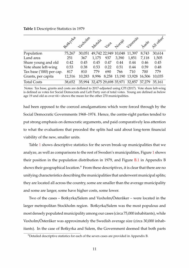
Table 1 Descriptive Statistics in 1979
Botkyrk
a
Vaxholm
Motal
a
Vara
Norsjö
Vännnäs
Åsele
All other∗
Population 75,267 30,051 49,742 22,949 10,048 11,397 8,743 30,614Land area 251 367 1,175 937 3,390 1,851 7,118 1,505Share young and old 0.42 0.45 0.45 0.47 0.44 0.44 0.46 0.45Vote share left-wing 0.53 0.38 0.53 0.22 0.51 0.44 0.59 0.48Tax base (’000) per cap. 817 810 779 690 766 710 700 779Grants, per capita 12,316 10,283 8,996 8,258 13,190 13,928 16,506 10,035Total Costs 38,652 35,994 32,475 29,698 35,971 32,857 37,279 35,161
Notes: Tax base, grants and costs are deflated to 2017-adjusted using CPI (2017). Vote share left-wingis defined as votes for Social Democrats and Left Party out of total votes. Young are defined as belowage 19 and old as over 64 ∗ shows the mean for the other 270 municipalities.
had been opposed to the coerced amalgamations which were forced through by the
Social Democratic Governments 1968–1974. Hence, the centre-right parties tended to
put strong emphasis on democratic arguments, and paid comparatively less attention
to what the evaluations that preceded the splits had said about long-term financial
viability of the new, smaller units.
Table 1 shows descriptive statistics for the seven break-up municipalities that we
analyze, as well as comparisons to the rest of Sweden’s municipalities, Figure 1 shows
their position in the population distribution in 1979, and Figure B.1 in Appendix B
shows their geographical location.9 From these descriptives, it is clear that there are no
unifying characteristics describing the municipalities that underwent municipal splits;
they are located all across the country, some are smaller than the average municipality
and some are larger, some have higher costs, some lower.
Two of the cases – Botkyrka/Salem and Vaxholm/Österåker – were located in the
larger metropolitan Stockholm region. Botkyrka/Salem was the most populous and
most densely populated municipality among our cases (circa 75,000 inhabitants), while
Vaxholm/Österåker was approximately the Swedish average size (circa 30,000 inhab-
itants). In the case of Botkyrka and Salem, the Government deemed that both parts
9Detailed descriptive statistics for each of the seven cases are provided in Appendix B.
11
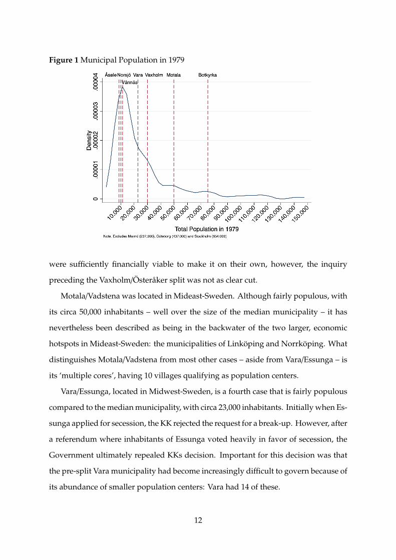
Figure 1 Municipal Population in 1979
were sufficiently financially viable to make it on their own, however, the inquiry
preceding the Vaxholm/Österåker split was not as clear cut.
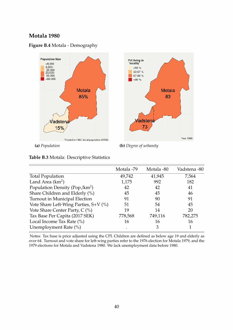
Motala/Vadstena was located in Mideast-Sweden. Although fairly populous, with
its circa 50,000 inhabitants – well over the size of the median municipality – it has
nevertheless been described as being in the backwater of the two larger, economic
hotspots in Mideast-Sweden: the municipalities of Linköping and Norrköping. What
distinguishes Motala/Vadstena from most other cases – aside from Vara/Essunga – is
its ‘multiple cores’, having 10 villages qualifying as population centers.
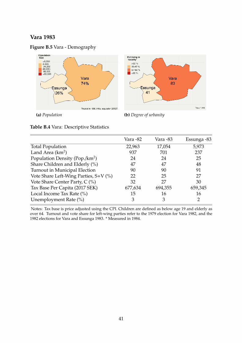
Vara/Essunga, located in Midwest-Sweden, is a fourth case that is fairly populous
compared to the median municipality, with circa 23,000 inhabitants. Initially when Es-
sunga applied for secession, the KK rejected the request for a break-up. However, after
a referendum where inhabitants of Essunga voted heavily in favor of secession, the
Government ultimately repealed KKs decision. Important for this decision was that
the pre-split Vara municipality had become increasingly difficult to govern because of
its abundance of smaller population centers: Vara had 14 of these.
12
The remaining three cases were all located in the more sparsely populated, rural
north of Sweden; i.e. the part of Sweden that has experienced severe de-population
over a long period of time. All three municipalities were originally small with respect
to population size (Norsjö/Malå 10,000, Vännäs/Bjurholm 11,000, Åsele/Dorotea circa
8,000), in addition to being sparsely populated.
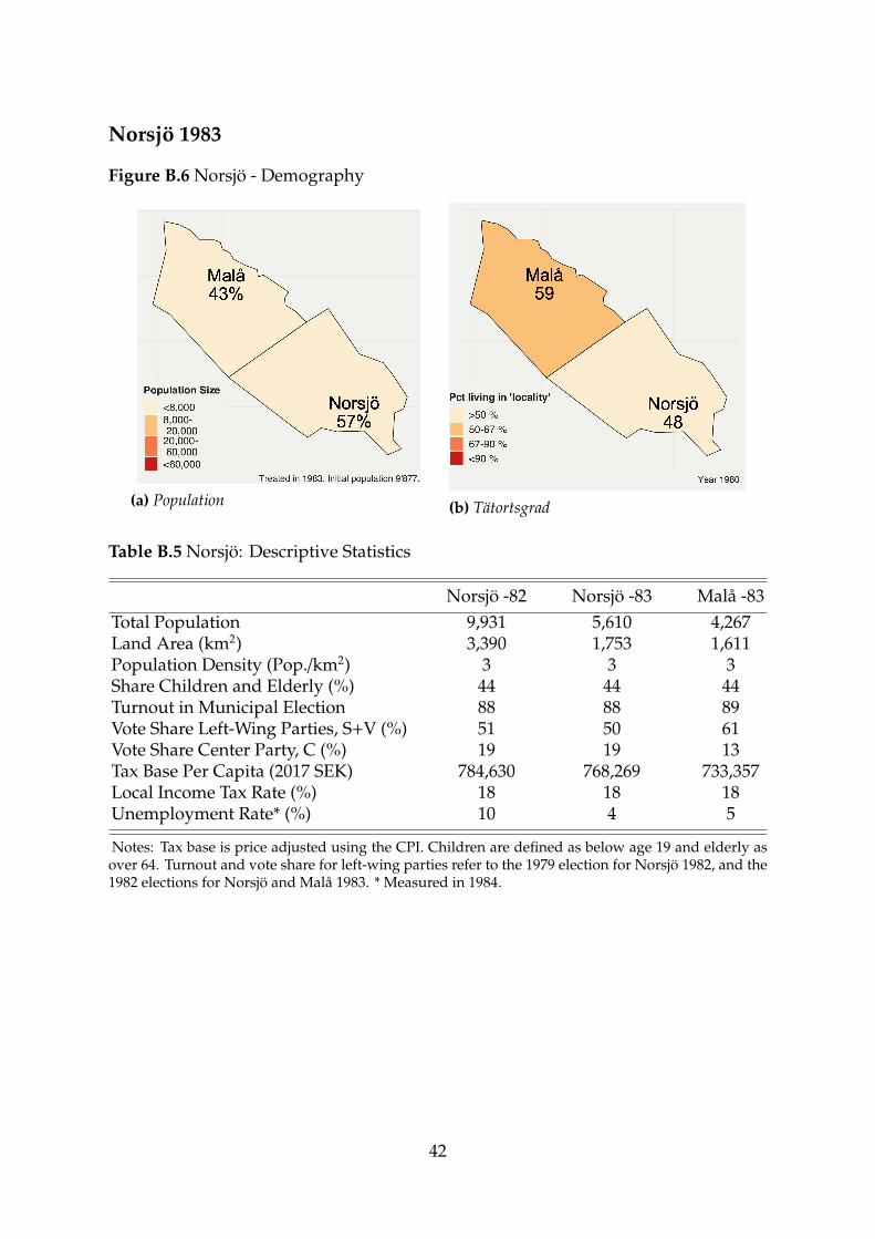
The main reasons underlying the Norsjö/Malå split were that Malå had rapidly lost
inhabitants post-merger partly due to loss of municipal job opportunities, and in addi-
tion that Malå felt that their needs were not listened or cared to by the administrative
center of Norsjö. The split was preceded by an inquiry that found that a separation
of the two would most likely have negative economic consequences for both Norsjö
and Malå. Despite this, and in light of strong support among the population in Malå,
the County Administrative Board of Västerbotten decided to advocate in favour of
a separation, and the Government choose to support the split, arguing that it was
motivated by democratic concerns.
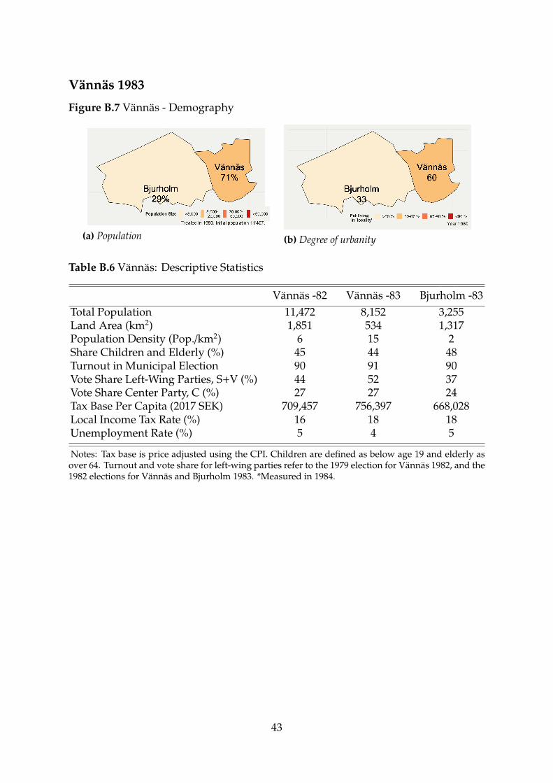
Considering Vännäs/Bjurholm, it is noteworthy that Bjurholm had experienced
population decline for several decades before the two municipalities were merged.
An inquiry that preceded the separation stated that a split-up could not be defended
economically, and none of the two parts alone was deemed sufficiently large to hold
its own financially in the long-term.10 In the end, the preferences of citizens once
again tipped the scale when the Government ruled – this time, though, not after
a referendum or poll, but through petitions that revealed a strong public support
backing the demand for separation.
In Åsele/Dorotea, the split was preceded by a poll which showed that a majority
in both parts were in favor of a split. During the brief period the merged Dorotea
municipality existed, politics was largely dominated by territorial belonging rather
than party politics: investments in one part of the new, larger municipality was
followed by conflict and negotiation about compensating the other part. Observers
10There was for example a fear that costs for elderly care would rise sharply in Bjurholm if it was tosecede.
13
have viewed it as a disadvantage for both Åsele and Dorotea that the Government’s
decision came late in the game – less than a year before the municipality was separated
into two units – which gave both parts limited time to prepare for the new order.
Since the seven cases we analyze have varying characteristics, and in addition are
located in distinctly different parts of Sweden – both metropolitan and rural regions
– it seems unreasonable to expect universal, homogeneous economic effects of break-
ups. On the contrary, first, as discussed in the theoretical section, we would expect
splits in metropolitan regions to be more prone to the positive effects of size-reduction
compared to splits in rural Sweden. Second, as noted, the different cases had very dif-
ferent starting points regarding pre-split population size. Third, there are important
differences when it comes to how many population centers the municipalities’ respec-
tive political and administrative centers needed to cater and be responsive to. Fourth,
the inquiries that preceded each separation made different evaluations concerning the
long-term financial viability of the respective post-merger parts; some getting a clear
thumbs up, and others projected a gloomy future.
5 Data
Our data covers all Swedish municipalities over the period 1974–1987, starting the first
year with the new municipal structure in place.11 After removing two municipalities12,
we are left with 276 municipalities in 1974, where seven municipalities were involved
in splits during the 1980s (two were split 1980, and five in 1983). To examine whether
municipalities forfeit economies of scale by splitting up, we study effects on total
municipal current costs per capita.13 In addition, we have collected information on
11We end in 1987 since Statistics Sweden made changes to the reporting of the survey that collectsmunicipal financial data in 1988, and therefore, complete compatibility with the years before cannot beguaranteed.
12We exclude Bara municipality, which only existed between 1974 and 1977, and Gotland, a munici-pality that also has the regional responsibilities of the Swedish meso-tier Landsting.
13In an earlier version of this paper, we also analyzed costs for municipal administration. Data on thisoutcome is only available for a shorter period (from 1978). It turned out that the empirical strategy wasnot successful in estimating counterfactual outcomes for the period preceding the municipal break-up
14
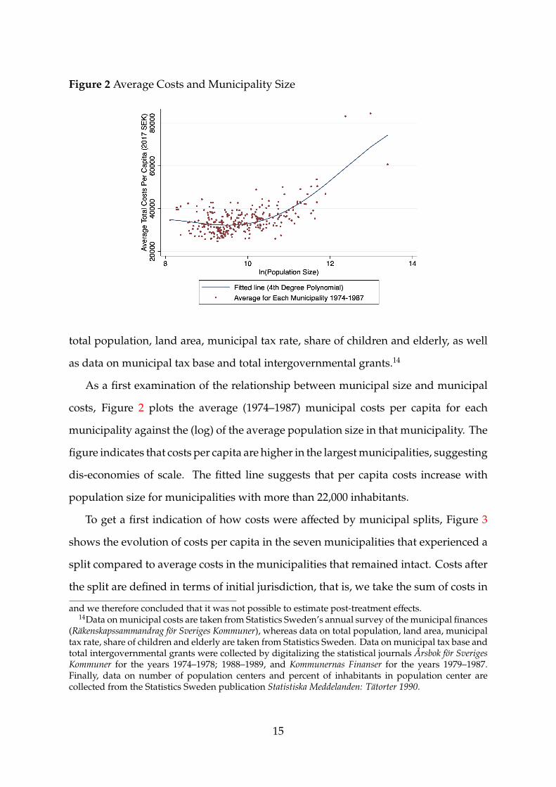
Figure 2 Average Costs and Municipality Size
total population, land area, municipal tax rate, share of children and elderly, as well
as data on municipal tax base and total intergovernmental grants.14
As a first examination of the relationship between municipal size and municipal
costs, Figure 2 plots the average (1974–1987) municipal costs per capita for each
municipality against the (log) of the average population size in that municipality. The
figure indicates that costs per capita are higher in the largest municipalities, suggesting
dis-economies of scale. The fitted line suggests that per capita costs increase with
population size for municipalities with more than 22,000 inhabitants.
To get a first indication of how costs were affected by municipal splits, Figure 3
shows the evolution of costs per capita in the seven municipalities that experienced a
split compared to average costs in the municipalities that remained intact. Costs after
the split are defined in terms of initial jurisdiction, that is, we take the sum of costs in
and we therefore concluded that it was not possible to estimate post-treatment effects.14Data on municipal costs are taken from Statistics Sweden’s annual survey of the municipal finances
(Räkenskapssammandrag för Sveriges Kommuner), whereas data on total population, land area, municipaltax rate, share of children and elderly are taken from Statistics Sweden. Data on municipal tax base andtotal intergovernmental grants were collected by digitalizing the statistical journals Årsbok för SverigesKommuner for the years 1974–1978; 1988–1989, and Kommunernas Finanser for the years 1979–1987.Finally, data on number of population centers and percent of inhabitants in population center arecollected from the Statistics Sweden publication Statistiska Meddelanden: Tätorter 1990.
15
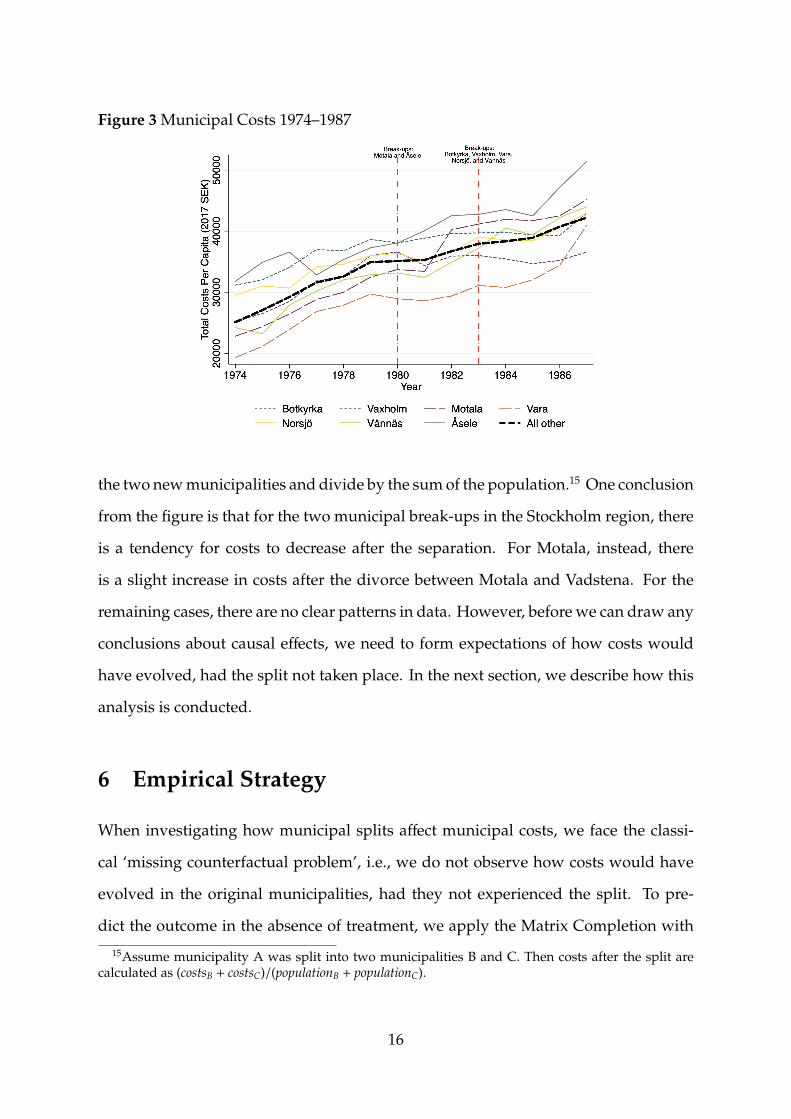
Figure 3 Municipal Costs 1974–1987
the two new municipalities and divide by the sum of the population.15 One conclusion
from the figure is that for the two municipal break-ups in the Stockholm region, there
is a tendency for costs to decrease after the separation. For Motala, instead, there
is a slight increase in costs after the divorce between Motala and Vadstena. For the
remaining cases, there are no clear patterns in data. However, before we can draw any
conclusions about causal effects, we need to form expectations of how costs would
have evolved, had the split not taken place. In the next section, we describe how this
analysis is conducted.
6 Empirical Strategy
When investigating how municipal splits affect municipal costs, we face the classi-
cal ‘missing counterfactual problem’, i.e., we do not observe how costs would have
evolved in the original municipalities, had they not experienced the split. To pre-
dict the outcome in the absence of treatment, we apply the Matrix Completion with
15Assume municipality A was split into two municipalities B and C. Then costs after the split arecalculated as (costsB + costsC)/(populationB + populationC).
16
Nuclear Norm Minimization (MC-NNM) suggested by Athey et al. (2017).16
6.1 The estimator
We consider the following model
Y = L∗ + γ∗i + δ∗t + εit (6.1)
where Y is the outcome under no-treatment, L∗ is a low rank matrix to be estimated,
γ∗i are unit fixed effects, δ∗t are time fixed effects, and εi,t is random noise. Athey et al.
(2017) suggest the following estimator
L = arg minL
{ 1|O|
∑i,t
(Yit − Lit − γi − δt)2 + λ||L||∗}
(6.2)
where O is a set of indices (i, t) corresponding to the non-missing entries in Yit, |O|
is the number of observed entries, PO(A) takes any matrix A and replaces all elements
whose indexes are not in O with 0, ||A||2F is the squared Fröbenius norm, and λ is the
regularization term on the nuclear norm ||L||∗.17
The estimator in equation 6.2 puts equal weight on all observed entities, regardless
of their similarity with the unobserved entities. Athey et al. (2017) suggest weighting
the observed units with their propensity scores in which case the weighed loss function
is given by
L = arg minL
{ 1|O|
∑i,t
eit
1 − eit(Yit − Lit − γi − δt)2 + λ||L||∗
}(6.3)
where eit are propensity scores, estimated through matrix completion.18
The estimated treatment effects on the treated (αit) are obtained by taking the
16Athey et al. (2017) derive theoretical bounds for their suggested estimator and provide MonteCarlo evidence showing that the estimator performs well in terms of RMSE, especially under staggeredadoption of treatment and when the pre-treatment period is short.
17The nuclear norm ||L||∗ is given by the sum of the singular values of L.18See section 8.3 in Athey et al. (2017) for details.
17
difference between the observed outcomes of a treated unit i in t ≥ T0, where T0 denotes
the first time period with treatment, and the imputed missing potential outcome:
αit = Yit − Yit (6.4)
6.2 Inference
How to conduct inference when applying matrix completion methods is not yet settled.
For that reason, we apply two different methods and interpret the overall results
holistically. First, we estimate confidence intervals through block bootstrapping,
selecting block length by the procedure suggested by Politis and White (2004). Second,
we calculate standardized p-values for the two-sided hypothesis test that αi,t = 0 for
each t ≥ T0, as suggested by Abadie et al. (2010) and Kumar and Liang (2018).19
pstd = Pr(|α j,t≥T0 |
RMSPEprej
≥|αi,t≥T0 |
RMSPEprei
)∀ j ∈ O (6.5)
where RMSPEpre =
√1/T0
∑t≤T0
(αt)2, j ∈ O and i 3 O.
Whereas the confidence intervals are calculated through bootstrapping, the stan-
dardized p-values instead estimate placebo effects for each of the non-treated munici-
palities, and then calculate the fraction of such effects greater than or equal to the effect
estimated for the treated unit, taking the match quality into account by standardizing
with the pre-treatment Root Mean Squared Error. The number of replications is there-
fore limited by the number of existing municipalities. Which of the two that performs
best in terms of size and power remains an open question.
19The idea is to estimate placebo effects for each non-treated unit in the sample and then calculatingthe fraction of such effects greater than or equal to the effect estimated for the treated unit. To take thematch quality into account, these are standardized by the pre-treatment Root Mean Squared Error.
18
6.3 Implementation
We estimate equation 6.3 using the algorithm suggested by Mazumder et al. (2010),
choosing the regularization parameter, λ, through cross-validation.20
When calculating the standardized p-values, we let each of the non-treated units
receive placebo treatment in 1980 and in 1983 one at a time. Thus, we compare
the treatment effects for the treated units, estimated jointly, to the placebo treatment
effects, estimated one by one. When estimating the placebo treatments, we remove
the treated municipalities from our sample.
7 Results
The main conclusion from the discussion in Section 2 is that the expected effect of
a municipal split on costs is likely to be case specific. The description of the seven
municipal break-ups which we study in this paper illustrates that our cases differ in
several theoretically relevant respects. We therefore allow for the effects to vary by
each municipal split.
7.1 Main results
Figure 4 shows the evolution over time of municipal costs in i) municipalities expe-
riencing a split (treated), ii) municipalities not experiencing a split (controls), and iii)
the predicted counterfactual for the treated municipalities. Figure 5 shows estimated
per-period effects (corresponding to equation 6.4) as well as 95-percent confidence
intervals.21 Municipal costs after the split are calculated as the sum of costs in the new
municipalities divided by the sum of the population in these municipalities.
20See Appendix C for a description of the algorithm as well for details in how we implement thecross-validation.
21Table D.1 presents the point estimates corresponding to Figure 5 as well as standardized p-values.Figures D.1 and D.2 compares estimated effects for the treated municipalities with estimated placebo-effects for non-treated municipalities.
19
The top panels of Figures 4 and 5 show the results for Botkyrka and Vaxholm,
both located in the larger Stockholm metropolitan region. For the pre-split period,
predicted counterfactual costs follow observed costs closely for the treated munici-
palities, indicating that the empirical strategy is successful. Once the municipalities
split, costs per capita begin to decline, being circa −5, 000 SEK lower four years after
the break-up. The confidence intervals in Figure 5 implies that the effect is statistically
significant at the five-percent level for years 1985–1987.
The next panels show that the break-ups do not imply lower costs for the more
peripheral and multi-cored municipalities of Motala and Vara. In Motala, per capita
costs instead increased to around 5,000 SEK. Despite relatively wide confidence inter-
vals, the effect is statistically significant in Motala for most years after the break-up.
In Vara, on the other hand, costs are unaffected in the first four years after the split,
but increase dramatically in year five. The point estimates for the pre-split period are
close to zero for both Vara and Motala, which indicates that the empirical strategy
works well.
The last panels show the results for the three smaller municipalities in the north
of Sweden. There is no indication that the split affected costs in Norsjö, whereas
per capita costs increased by around 3,500 SEK as a consequence of the break-up of
Vännäs. For Norsjö, there are indications that the empirical strategy is less successful
in predicting the counterfactual outcome for the first two years, but for 1976–1982,
predicted costs follow observed costs closely. For Åsele, the empirical strategy is less
successful, and the estimates for the pre-split period are relatively large and fluctuate
between being (borderline) statistically significant positive and statistically significant
negative. Specifically, Figure 4 indicates that something caused actual costs to decrease
sharply in 1977.
20
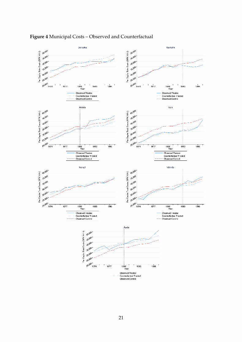
Figure 4 Municipal Costs – Observed and Counterfactual
21
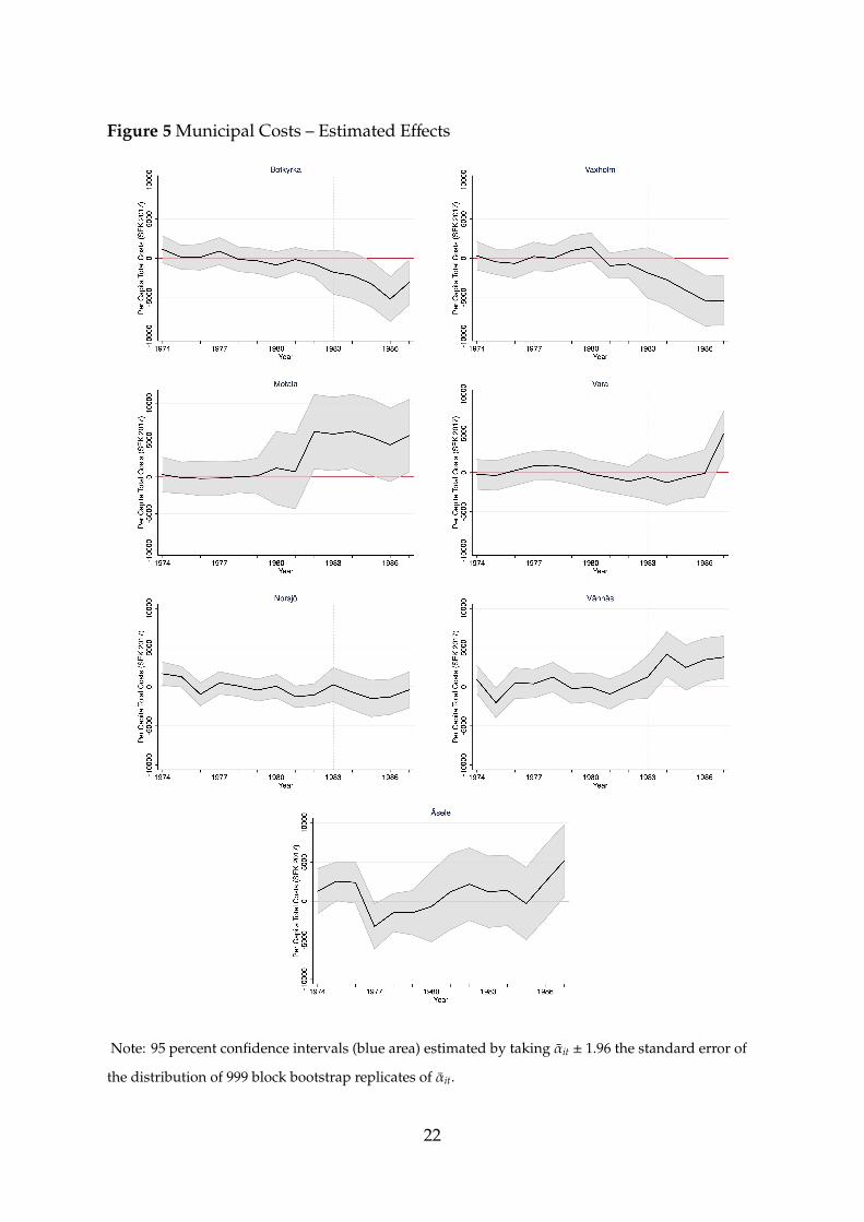
Figure 5 Municipal Costs – Estimated Effects
Note: 95 percent confidence intervals (blue area) estimated by taking αit ± 1.96 the standard error of
the distribution of 999 block bootstrap replicates of αit.
22
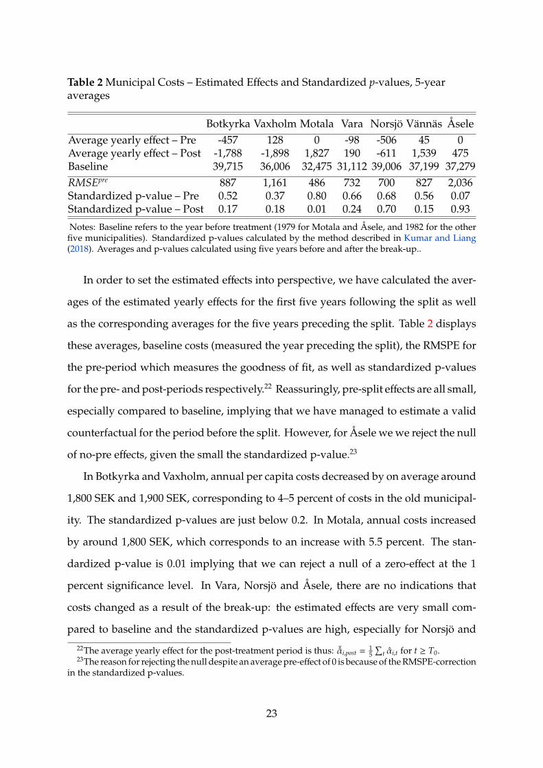
Table 2 Municipal Costs – Estimated Effects and Standardized p-values, 5-yearaverages
Botkyrka Vaxholm Motala Vara Norsjö Vännäs ÅseleAverage yearly effect – Pre -457 128 0 -98 -506 45 0Average yearly effect – Post -1,788 -1,898 1,827 190 -611 1,539 475Baseline 39,715 36,006 32,475 31,112 39,006 37,199 37,279RMSEpre 887 1,161 486 732 700 827 2,036Standardized p-value – Pre 0.52 0.37 0.80 0.66 0.68 0.56 0.07Standardized p-value – Post 0.17 0.18 0.01 0.24 0.70 0.15 0.93
Notes: Baseline refers to the year before treatment (1979 for Motala and Åsele, and 1982 for the otherfive municipalities). Standardized p-values calculated by the method described in Kumar and Liang(2018). Averages and p-values calculated using five years before and after the break-up..
In order to set the estimated effects into perspective, we have calculated the aver-
ages of the estimated yearly effects for the first five years following the split as well
as the corresponding averages for the five years preceding the split. Table 2 displays
these averages, baseline costs (measured the year preceding the split), the RMSPE for
the pre-period which measures the goodness of fit, as well as standardized p-values
for the pre- and post-periods respectively.22 Reassuringly, pre-split effects are all small,
especially compared to baseline, implying that we have managed to estimate a valid
counterfactual for the period before the split. However, for Åsele we we reject the null
of no-pre effects, given the small the standardized p-value.23
In Botkyrka and Vaxholm, annual per capita costs decreased by on average around
1,800 SEK and 1,900 SEK, corresponding to 4–5 percent of costs in the old municipal-
ity. The standardized p-values are just below 0.2. In Motala, annual costs increased
by around 1,800 SEK, which corresponds to an increase with 5.5 percent. The stan-
dardized p-value is 0.01 implying that we can reject a null of a zero-effect at the 1
percent significance level. In Vara, Norsjö and Åsele, there are no indications that
costs changed as a result of the break-up: the estimated effects are very small com-
pared to baseline and the standardized p-values are high, especially for Norsjö and
22The average yearly effect for the post-treatment period is thus: ¯αi,post = 15
∑t αi,t for t ≥ T0.
23The reason for rejecting the null despite an average pre-effect of 0 is because of the RMSPE-correctionin the standardized p-values.
23
Åsele. In Vännäs, on the other hand, yearly per capita costs increased by on average
around 1,500 SEK per capita as a result fo the break-up, corresponding to an increase
of four percent. The standardized p-value is 0.15.
As is clear from the results thus far, the estimated effects of municipal splits vary
significantly from case to case. In, e.g. Botkyrka and Vaxholm our results point at
decreasing costs per capita as a consequence of the break-ups, whereas in Motala
and Vännäs per capita costs seem to have increased. Hence, assuming homogeneous
treatment effects of municipal splits (and mergers), as has been done in much of the
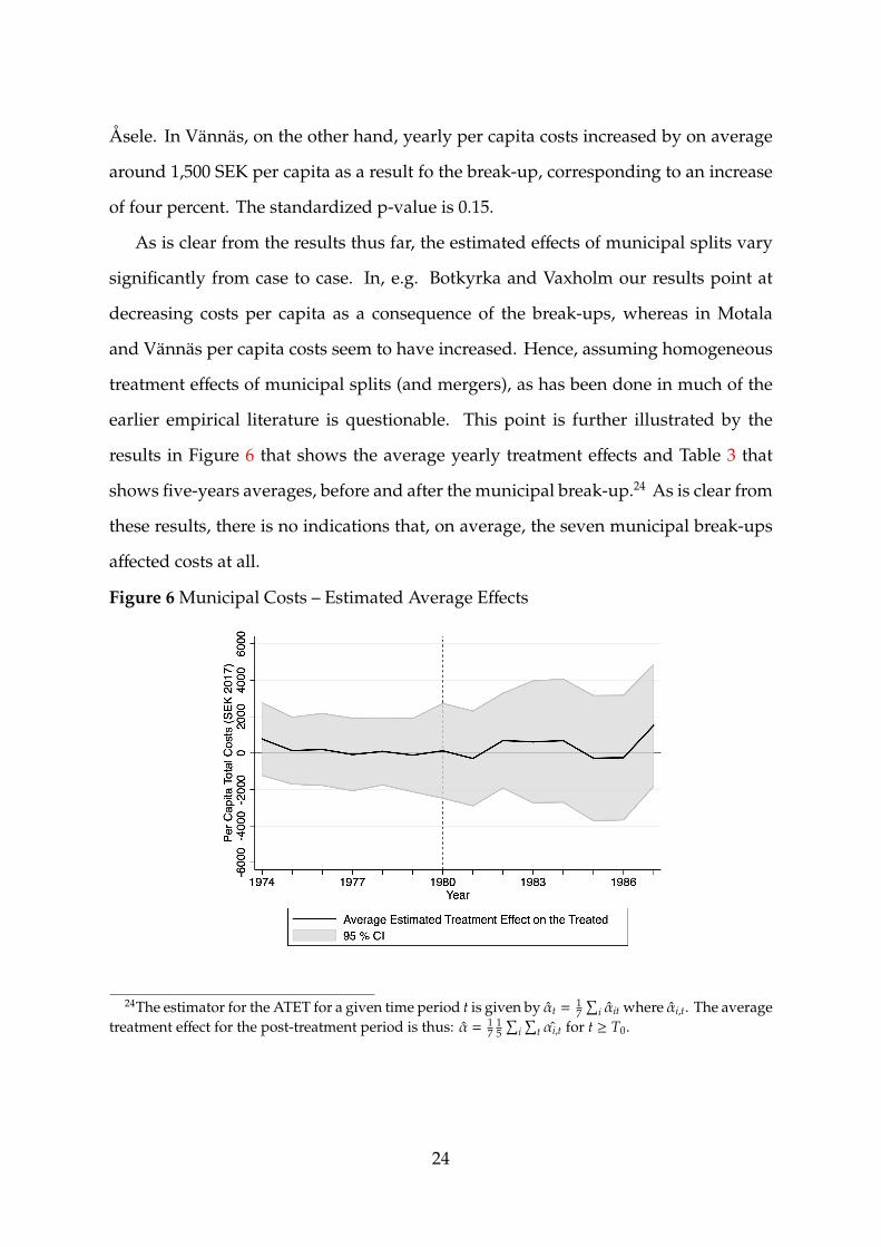
earlier empirical literature is questionable. This point is further illustrated by the
results in Figure 6 that shows the average yearly treatment effects and Table 3 that
shows five-years averages, before and after the municipal break-up.24 As is clear from
these results, there is no indications that, on average, the seven municipal break-ups
affected costs at all.
Figure 6 Municipal Costs – Estimated Average Effects
24The estimator for the ATET for a given time period t is given by αt = 17
∑i αit where αi,t. The average
treatment effect for the post-treatment period is thus: α = 17
15
∑i∑
t αi,t for t ≥ T0.
24
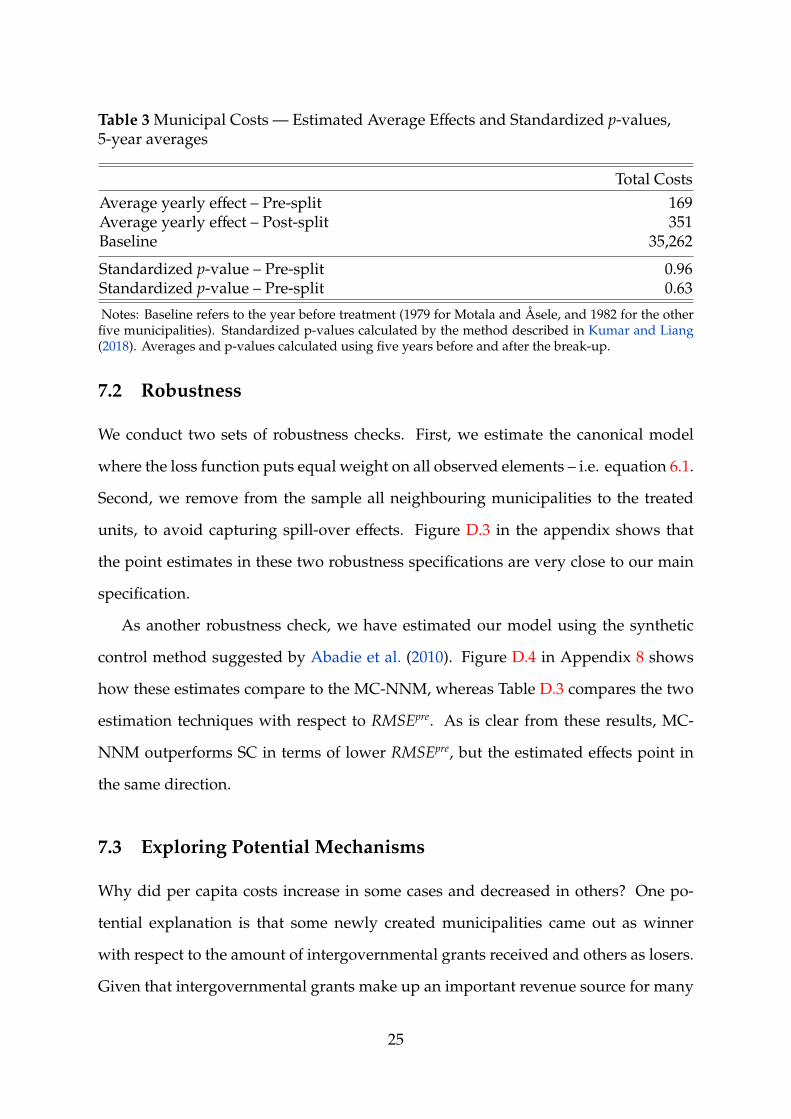
Table 3 Municipal Costs — Estimated Average Effects and Standardized p-values,5-year averages
Total CostsAverage yearly effect – Pre-split 169Average yearly effect – Post-split 351Baseline 35,262
Standardized p-value – Pre-split 0.96Standardized p-value – Pre-split 0.63
Notes: Baseline refers to the year before treatment (1979 for Motala and Åsele, and 1982 for the otherfive municipalities). Standardized p-values calculated by the method described in Kumar and Liang(2018). Averages and p-values calculated using five years before and after the break-up.
7.2 Robustness
We conduct two sets of robustness checks. First, we estimate the canonical model
where the loss function puts equal weight on all observed elements – i.e. equation 6.1.
Second, we remove from the sample all neighbouring municipalities to the treated
units, to avoid capturing spill-over effects. Figure D.3 in the appendix shows that
the point estimates in these two robustness specifications are very close to our main
specification.
As another robustness check, we have estimated our model using the synthetic
control method suggested by Abadie et al. (2010). Figure D.4 in Appendix 8 shows
how these estimates compare to the MC-NNM, whereas Table D.3 compares the two
estimation techniques with respect to RMSEpre. As is clear from these results, MC-
NNM outperforms SC in terms of lower RMSEpre, but the estimated effects point in
the same direction.
7.3 Exploring Potential Mechanisms
Why did per capita costs increase in some cases and decreased in others? One po-
tential explanation is that some newly created municipalities came out as winner
with respect to the amount of intergovernmental grants received and others as losers.
Given that intergovernmental grants make up an important revenue source for many
25
municipalities, this seems like a natural candidate. However, Table D.2 and Figure D.5
in Appendix D show that the estimated effects on grants are both economically and
statistically insignificant. One explanation for the absence of an effect is most likely
that 80 percent of total grants were targeted during the studied period, and targeted
grants are – as opposed to general grants – unaffected by changes to the demographic
composition.
So far we have discussed costs per capita as mainly a result of the cost-efficiency of
municipal service production. However, it is likely that citizen’s preferences matter
as well, especially since we lack any way of controlling for the quality of service
provision. As is clear from the discussion in Section 4, the municipal splits we study
were typically motivated by democratic arguments. If the political majority changed
in one of the newly formed municipalities following the break-up, we might expect
that costs change as a result. Figure 7 shows the vote share for the left-wing parties
(panel to the left) and per capita costs (panel to the right) in the pre-split municipality
and in the two newly formed municipalities after the split.
Focusing first on the two municipalities for which we find decreasing costs,
Botkyrkan and Vaxholm, the figure shows that the political majority changed from
a left-wing in the old jurisdiction Botkyrka to a right-wing in the new jurisdiction
Salem, which would be in line with lower municipal spending in Salem. Perhaps
somewhat surprisingly, costs nevertheless basically followed the same trajectories af-
ter the break-up into the two new units.25 The break-up of Vaxholm did not result
in changing political majority, although the support for the left wing was somewhat
higher in Vaxholm once Österåker broke out of the municipality.
Turning next to Motala, where we find evidence of increasing per capita costs as
a result of the split, the left coalition had a majority before the split, and increased its
support in the remaining part once Vadstena broke out, whereas it lost its majority
in the newly formed municipality Vadstena. After the split, per capita costs are
25However, these results do not inform us what would have happened if Salem had remained in thelarger municipality. This was the task of the estimated effects in Figure 5 above.
26
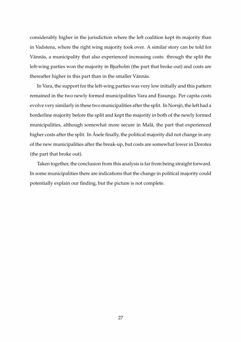
considerably higher in the jurisdiction where the left coalition kept its majority than
in Vadstena, where the right wing majority took over. A similar story can be told for
Vännäs, a municipality that also experienced increasing costs: through the split the
left-wing parties won the majority in Bjurholm (the part that broke out) and costs are
thereafter higher in this part than in the smaller Vännäs.
In Vara, the support for the left-wing parties was very low initially and this pattern
remained in the two newly formed municipalities Vara and Essunga. Per capita costs
evolve very similarly in these two municipalities after the split. In Norsjö, the left had a
borderline majority before the split and kept the majority in both of the newly formed
municipalities, although somewhat more secure in Malå, the part that experienced
higher costs after the split. In Åsele finally, the political majority did not change in any
of the new municipalities after the break-up, but costs are somewhat lower in Dorotea
(the part that broke out).
Taken together, the conclusion from this analysis is far from being straight forward.
In some municipalities there are indications that the change in political majority could
potentially explain our finding, but the picture is not complete.
27
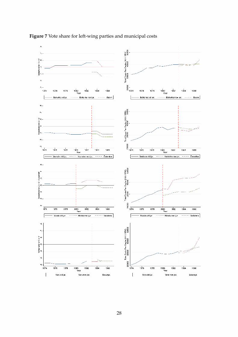
Figure 7 Vote share for left-wing parties and municipal costs
28
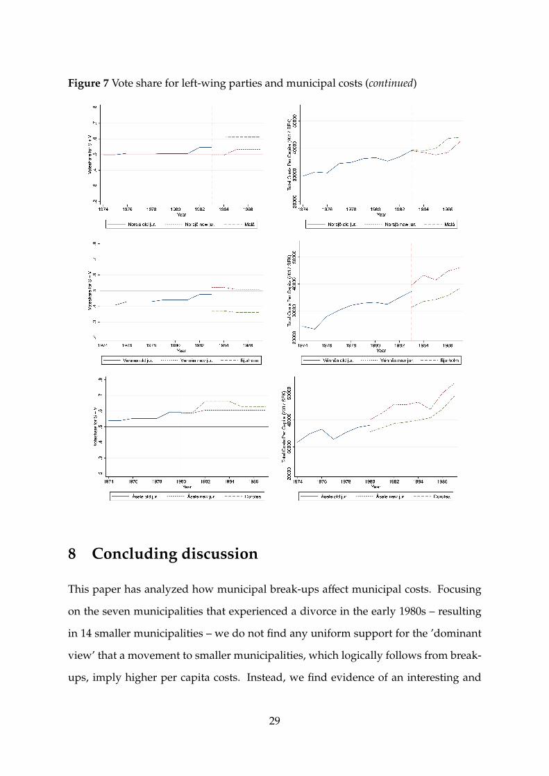
Figure 7 Vote share for left-wing parties and municipal costs (continued)
8 Concluding discussion
This paper has analyzed how municipal break-ups affect municipal costs. Focusing
on the seven municipalities that experienced a divorce in the early 1980s – resulting
in 14 smaller municipalities – we do not find any uniform support for the ’dominant
view’ that a movement to smaller municipalities, which logically follows from break-
ups, imply higher per capita costs. Instead, we find evidence of an interesting and
29
intriguing heterogeneity in outcomes: costs increase in some cases, are unaffected in
others, but decrease elsewhere. More specifically, costs have a tendency to decrease in
densely populated areas close to the metropolitan Greater Stockholm region, whereas
splits tend to lead to unaffected or higher costs in the more sparsely populated regions
of Sweden.
The decreasing costs in the metropolitan Stockholm cases can be understood both
in light of the polycentric view, stating that splits in metropolitan regions could lead
to cost-efficiency as a result of increased competition between municipalities for tax-
payers, as well as the idea of a U-shaped cost function, where their relatively large
initial size might have been associated with dis-economies of scale. The increasing
costs in Motala and Vännäs could potentially also be understood in light of the poly-
centric view. For Vännäs, however, another possibility is that the break-up allowed for
a better matching between political preferences and policy, when the left-wing parties
– who are more prone to spending – won the majority in one of the two splitting parts.
These heterogeneous empirical findings point to the importance of evaluating po-
tential effects of territorial reforms – municipal break-ups as well as amalgamations –
on a case-by-case basis. If we had treated our cases in the aggregate and ignored the
potential heterogeneity in effects, we would have reached the erroneous conclusion
that the territorial reforms that took place in Sweden in the early 1980s did not af-
fect municipal costs. Our findings, therefore, underscore the perils of policy makers’
propagating territorial reforms as ‘universal’ or ‘one size fits all’ solutions to complex
societal challenges. By implication, the findings also highlight the difficulty in draw-
ing general conclusions about their effects. In fact, it could make sense to advocate
splits in certain cases and parts of a country, and amalgamations in others. Conse-
quently, although this paper has had its focus on break-ups, our findings rejoin the
overall results from the empirical literature on amalgamations, which underline the
naivety of policy makers placing their bets on that sweeping and all-encompassing
amalgamation reforms will save costs.
30
References
Abadie, A., Diamond, A., and Hainmueller, J. Synthetic Control Methods for Compar-
ative Case Studies: Estimating the Effect of California’s Tobacco Control Program.
Journal of the American Statistical Association, 105(490):493–505, 2010.
Allers, M. A. and Geertsema, J. B. The Effects of Local Government Amalgamation on
Public Spending, Taxation, and Service Levels: Evidence from 15 Years of Municipal
Consolidation. Journal of Regional Science, 56(4):659–682, 2016.
Andrews, R. Vertical Consolidation and Financial Sustainability: Evidence from
English Local Government. Environment and Planning C: Government and Policy, 33
(6):1518–1545, 2015.
Athey, S., Imbens, G., Bayati, S., Doudchenko, N., and Khosravi, K. Matrix Completion
Methods for Causal Panel Data Models. ArXiv Preprint, (1710.10251):1–49, 2017.
Blesse, S. and Baskaran, T. Do Municipal Mergers Reduce Costs? Evidence from a
German Federal State. Regional Science and Urban Economics, 59:54–74, 2016.
Blom-Hansen, J., Houlberg, K., and Serritzlew, S. Size, Democracy, and the Economic
Costs of Running the Political System. American Journal of Political Science, 58(4):
790–803, 2014.
Blom-Hansen, J., Houlberg, K., and Treisman, D. Jurisdiction Size and Local Gov-
ernment Policy Expenditure: Assessing the Effect of Municipal Amalgamation.
American Political Science Review, 110(4), 2016.
Bordignon, M., Cerniglia, F., and Revelli, F. Yardstick Competition in Intergovern-
mental Relationships: Theory and Empirical Predictions. Economics Letters, 83(3):
325–333, 2004.
Bouckaert, G. and Kuhlman, S. Introduction: Comparing Local Public Sector Reforms:
31
Institutional Policies in Context. In Bouckaert, G. and Kuhlman, S., editors, Local
Public Sector Reforms in Times Of Crisis. Cham: Palgrave Macmillan, 2016.
Breunig, R. and Rocaboy, Y. Per-Capita Public Expenditures and Population Size: A
Non-Parametric Analysis Using French Data. Public Choice, 136(3/4):429–445, 2008.
Cobban, T. W. Bigger is Better: Reducing the Cost of Local Administration by In-
creasing Jurisdiction Size in Ontario, Canada, 1995–2010. Urban Affairs Review, 55
(2):462–500, 2019.
Cristaller, W. Central Places in Southern Germany. Prentice-Hall, Englewood Cliffs, N.J.,
1966.
Dahl, R. and Tufte, E. Size and Democracy (The Politics of the Smaller European Democra-
cies). Stanford Paperbacks. Stanford University Press, 1973.
de Souza, S. V., Dollery, B. E., and Kortt, M. A. De-amalgamation in Action: The
Queensland Experience. Public Management Review, 17(10):1403–1424, 2015.
Dollery, B. E. and Byrnes, J. Do Economies of Scale Exist in Australian Local Govern-
ment? A Review of Evidence. Urban Policy and Research, 20(4):391–414, 2002.
Dollery, B. E., Grant, B., and Kortt, M. A. A Normative Model for Local Government
De-amalgamation in Australia. Australian Journal of Political Science, 46(4):601–615,
2011.
Erlingsson, G. Modelling Secessions from Municipalities. Scandinavian Political Stud-
ies, 28(2):141–159, 2005.
Fox, W. F. and Gurley, T. Will Consolidation Improve Sub-National Governments?
World Bank Working Paper, 3913, 2006.
Gendzwill, A., Kurniewicz, A., and Swianiewicz, P. The impact of municipal territorial
reforms on the economic performance of local governments. a systematic review of
quasi-experimental studies. Space and Polity, pages 1–20, 2020.
32
Harjunen, O., Saarimaa, T., and Tukiainen, J. Political Representation and Effects of
Municipal Mergers. Political Science Research and Methods, page 1–17, 2019.
Hirsch, W. Expenditure Implications of Metropolitan Growth and Consolidation.
Review of Economics and Statistics, 41(3):232–41, 1959.
Kolam, K. and Ekman, C. Kommundelningar: Erfarenheter och Utfall. Umeå Universitet,
Umeå, 1992.
Kumar, A. and Liang, C.-Y. Labor Market Effects of Credit Constraints: Evidence from
a Natural Experiment. Federal Reserve Bank of Dallas, Working Papers, 2018(1810),
2018.
Ladner, A., Keuffer, N., and Baldersheim, H. Measuring local Autonomy in 39 Coun-
tries. Regional and Federal Studies, 26(3):321–357, 2016.
Lima, R. C. d. A., Neto, S., and da Mota Raul. Secession of Municipalities and
Economies of Scale: Evidence from Brazil. Journal of Regional Science, 58(1):159–180,
2018.
Mazumder, R., Hastie, T., and Tibsirani, R. Spectral Regularization Algorithms for
Learning Large Incomplete Matrices. Journal of Machine Learning Research, 11:2287–
2322, 2010.
McQuestin, D., Drew, J., and Dollery, B. Do Municipal Mergers Improve Technical Effi-
ciency? An Empirical Analysis of the 2008 Queensland Municipal Merger Program.
Australian Journal of Public Administration, 77(3):442–455, 2018.
Miyazaki, T. Examining the Relationship Between Municipal Consolidation and Cost
Reduction: an Instrumental Variable Approach. Applied Economics, 50(10):1108–
1121, 2018.
Moisio, A. and Uusitalo, R. The Impact of Municipal Mergers on Local Public Expen-
ditures in Finland. Public Finance and Management, 13(3):148–166, 2013.
33
Nielsen, P. Kommunindelning och Demokrati. Om Sammanläggning och Delning av
Kommuner i Sverige (Municipality Division and Democracy. Amalgamation and
Secession of Municipalities in Sweden). Acta Universitatis Upsaliensis, 157:367, 2003.
Oates, W. E. Fiscal Federalism. Harcourt Brace Jovanovich, New York, 1972.
Ostrom, V., Tiebout, C. M., and Warren, R. The Organization of Government in
Metropolitan Areas: a Theoretical Inquiry. The American Political Science Review, 55
(4):831–842, 1961.
Politis, D. N. and White, H. Automatic Block-Length Selection for the Dependent
Bootstrap. Econometric Reviews, 23(1):53–70, 2004.
Reingewertz, Y. Do Municipal Amalgamations Work? Evidence from Municipalities
in Israel. Journal of Urban Economics, 72(2-3):240–251, 2012.
Roesel, F. Do Mergers of Large Local Governments Reduce Expenditures? – Evidence
from Germany using the Synthetic Control Method. European Journal of Political
Economy, 50(October):22–36, 2017.
Sellers, J. M. and Lidström, A. Decentralization, Local Government, and the Welfare
State. Governance, 20(4):609–632, 2007.
SOU 1961:9. Principer för en Ny Kommunindelning (Principles for a New Municipal
Division). Technical report, Stockholm: Inrikesdepartementet, 1961.
Swianiewicz, P. and Łukomska, J. Is Small Beautiful? The Quasi-experimental Analy-
sis of the Impact of Territorial Fragmentation on Costs in Polish Local Governments.
Urban Affairs Review, 55(3):832–855, 2019.
Tavares, A. F. Municipal Amalgamations and their Effects: A Literature Review.
Miscellanea Geographica: Regional Studies on Development, 22(1):5–15, 2018.
34
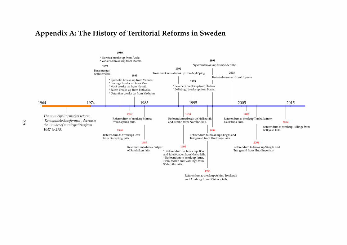
Appendix A: The History of Territorial Reforms in Sweden
The municipality merger reform,’Kommunblocksreformen’, decreasesthe number of municipalities from1047 to 278.
1964 1974 1985 1995 2005 2015
1980
* Dorotea breaks up from Åsele.* Vadstena breaks up from Motala.
1983
* Bjurholm breaks up from Vännäs.* Essunga breaks up from Vara.* Malå breaks up from Norsjö.* Salem breaks up from Botkyrka.* Österåker breaks up from Vaxholm.
1977
Bara mergeswith Svedala
1999
Nykvarn breaks up from Södertälje.1992
Trosa and Gnesta break up from Nyköping.
1995
* Lekeberg breaks up from Örebro.* Bollebygd breaks up from Borås.
2003
Knivsta breaks up from Uppsala.
1985
Referendum to break out partof Sandviken fails.
1980
Referendum to break up Hovafrom Gullspång fails.
1982
Referendum to break up Märstafrom Sigtuna fails.
1998
Referendum to break up Askim, Torslandaand Älvsborg from Göteborg fails.
1993
* Referendum to break up Booand Saltsjöbaden from Nacka fails.* Referendum to break up Järna,Hölö-Mörkö and Vårdinge fromSödertälje fails.
1999
Referendum to break up Skogås andTrångsund from Huddinge fails.
1994
Referendum to break up Hallstavikand Rimbo from Nortälje fails.
2008
Referendum to break up Skogås andTrångsund from Huddinge fails.
2006
Referendum to break up Torshälla fromEskilstuna fails. 2014
Referendum to break up Tullinge fromBotkyrka fails.
35

36
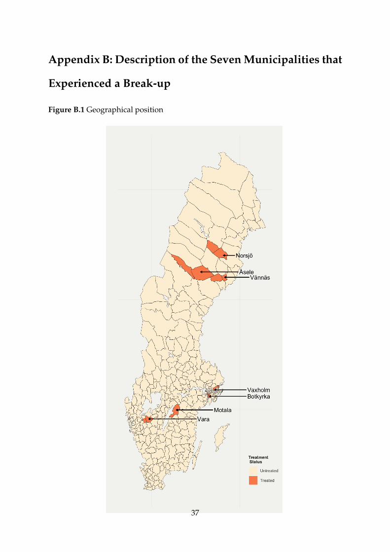
Appendix B: Description of the Seven Municipalities that
Experienced a Break-up
Figure B.1 Geographical position
37
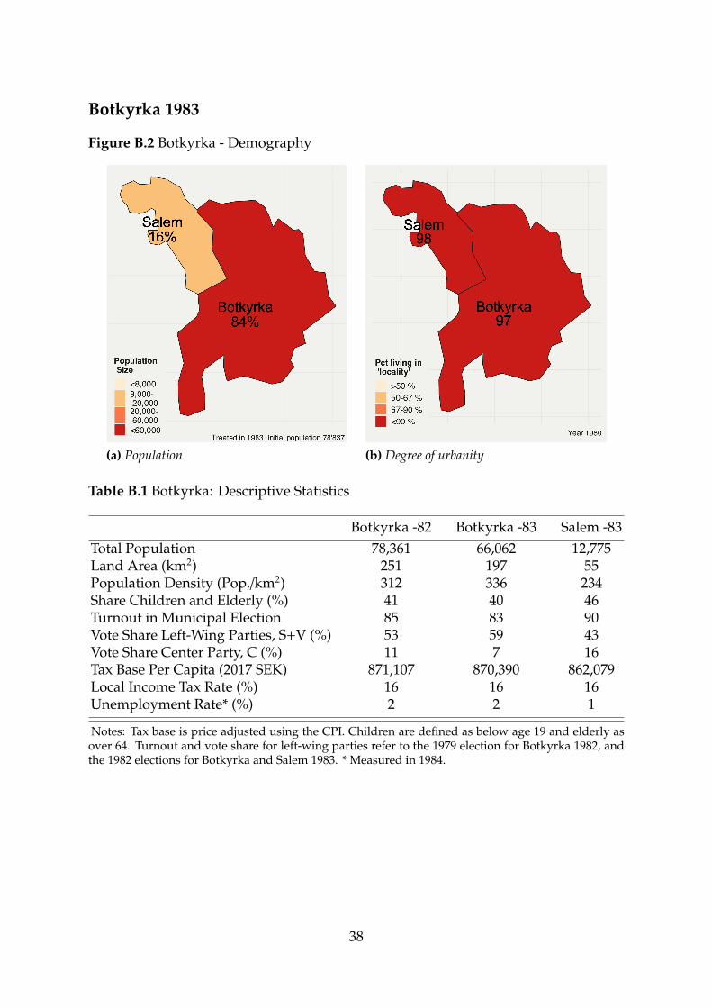
Botkyrka 1983
Figure B.2 Botkyrka - Demography
(a) Population (b) Degree of urbanity
Table B.1 Botkyrka: Descriptive Statistics
Botkyrka -82 Botkyrka -83 Salem -83Total Population 78,361 66,062 12,775Land Area (km2) 251 197 55Population Density (Pop./km2) 312 336 234Share Children and Elderly (%) 41 40 46Turnout in Municipal Election 85 83 90Vote Share Left-Wing Parties, S+V (%) 53 59 43Vote Share Center Party, C (%) 11 7 16Tax Base Per Capita (2017 SEK) 871,107 870,390 862,079Local Income Tax Rate (%) 16 16 16Unemployment Rate* (%) 2 2 1
Notes: Tax base is price adjusted using the CPI. Children are defined as below age 19 and elderly asover 64. Turnout and vote share for left-wing parties refer to the 1979 election for Botkyrka 1982, andthe 1982 elections for Botkyrka and Salem 1983. * Measured in 1984.
38
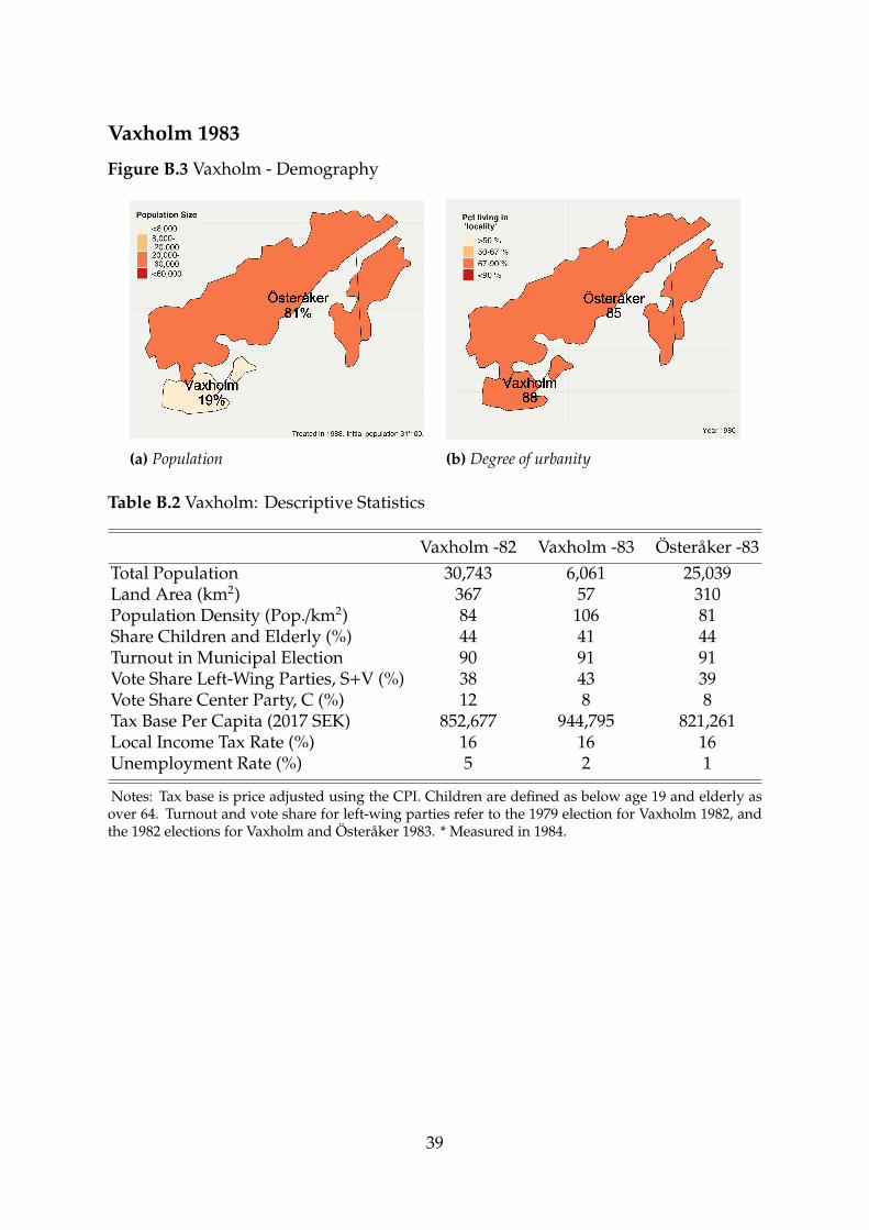
Vaxholm 1983
Figure B.3 Vaxholm - Demography
(a) Population (b) Degree of urbanity
Table B.2 Vaxholm: Descriptive Statistics
Vaxholm -82 Vaxholm -83 Österåker -83Total Population 30,743 6,061 25,039Land Area (km2) 367 57 310Population Density (Pop./km2) 84 106 81Share Children and Elderly (%) 44 41 44Turnout in Municipal Election 90 91 91Vote Share Left-Wing Parties, S+V (%) 38 43 39Vote Share Center Party, C (%) 12 8 8Tax Base Per Capita (2017 SEK) 852,677 944,795 821,261Local Income Tax Rate (%) 16 16 16Unemployment Rate (%) 5 2 1
Notes: Tax base is price adjusted using the CPI. Children are defined as below age 19 and elderly asover 64. Turnout and vote share for left-wing parties refer to the 1979 election for Vaxholm 1982, andthe 1982 elections for Vaxholm and Österåker 1983. * Measured in 1984.
39
Motala 1980
Figure B.4 Motala - Demography
(a) Population (b) Degree of urbanity
Table B.3 Motala: Descriptive Statistics
Motala -79 Motala -80 Vadstena -80Total Population 49,742 41,945 7,564Land Area (km2) 1,175 992 182Population Density (Pop./km2) 42 42 41Share Children and Elderly (%) 45 45 46Turnout in Municipal Election 91 90 91Vote Share Left-Wing Parties, S+V (%) 51 54 45Vote Share Center Party, C (%) 19 14 20Tax Base Per Capita (2017 SEK) 778,568 749,116 782,275Local Income Tax Rate (%) 16 16 16Unemployment Rate (%) . 3 1
Notes: Tax base is price adjusted using the CPI. Children are defined as below age 19 and elderly asover 64. Turnout and vote share for left-wing parties refer to the 1976 election for Motala 1979, and the1979 elections for Motala and Vadstena 1980. We lack unemployment data before 1980.
40
Vara 1983
Figure B.5 Vara - Demography
(a) Population (b) Degree of urbanity
Table B.4 Vara: Descriptive Statistics
Vara -82 Vara -83 Essunga -83Total Population 22,963 17,054 5,973Land Area (km2) 937 701 237Population Density (Pop./km2) 24 24 25Share Children and Elderly (%) 47 47 48Turnout in Municipal Election 90 90 91Vote Share Left-Wing Parties, S+V (%) 22 25 27Vote Share Center Party, C (%) 32 27 30Tax Base Per Capita (2017 SEK) 677,634 694,355 659,345Local Income Tax Rate (%) 15 16 16Unemployment Rate (%) 3 3 2
Notes: Tax base is price adjusted using the CPI. Children are defined as below age 19 and elderly asover 64. Turnout and vote share for left-wing parties refer to the 1979 election for Vara 1982, and the1982 elections for Vara and Essunga 1983. * Measured in 1984.
41
Norsjö 1983
Figure B.6 Norsjö - Demography
(a) Population (b) Tätortsgrad
Table B.5 Norsjö: Descriptive Statistics
Norsjö -82 Norsjö -83 Malå -83Total Population 9,931 5,610 4,267Land Area (km2) 3,390 1,753 1,611Population Density (Pop./km2) 3 3 3Share Children and Elderly (%) 44 44 44Turnout in Municipal Election 88 88 89Vote Share Left-Wing Parties, S+V (%) 51 50 61Vote Share Center Party, C (%) 19 19 13Tax Base Per Capita (2017 SEK) 784,630 768,269 733,357Local Income Tax Rate (%) 18 18 18Unemployment Rate* (%) 10 4 5
Notes: Tax base is price adjusted using the CPI. Children are defined as below age 19 and elderly asover 64. Turnout and vote share for left-wing parties refer to the 1979 election for Norsjö 1982, and the1982 elections for Norsjö and Malå 1983. * Measured in 1984.
42
Vännäs 1983
Figure B.7 Vännäs - Demography
(a) Population (b) Degree of urbanity
Table B.6 Vännäs: Descriptive Statistics
Vännäs -82 Vännäs -83 Bjurholm -83Total Population 11,472 8,152 3,255Land Area (km2) 1,851 534 1,317Population Density (Pop./km2) 6 15 2Share Children and Elderly (%) 45 44 48Turnout in Municipal Election 90 91 90Vote Share Left-Wing Parties, S+V (%) 44 52 37Vote Share Center Party, C (%) 27 27 24Tax Base Per Capita (2017 SEK) 709,457 756,397 668,028Local Income Tax Rate (%) 16 18 18Unemployment Rate (%) 5 4 5
Notes: Tax base is price adjusted using the CPI. Children are defined as below age 19 and elderly asover 64. Turnout and vote share for left-wing parties refer to the 1979 election for Vännäs 1982, and the1982 elections for Vännäs and Bjurholm 1983. *Measured in 1984.
43
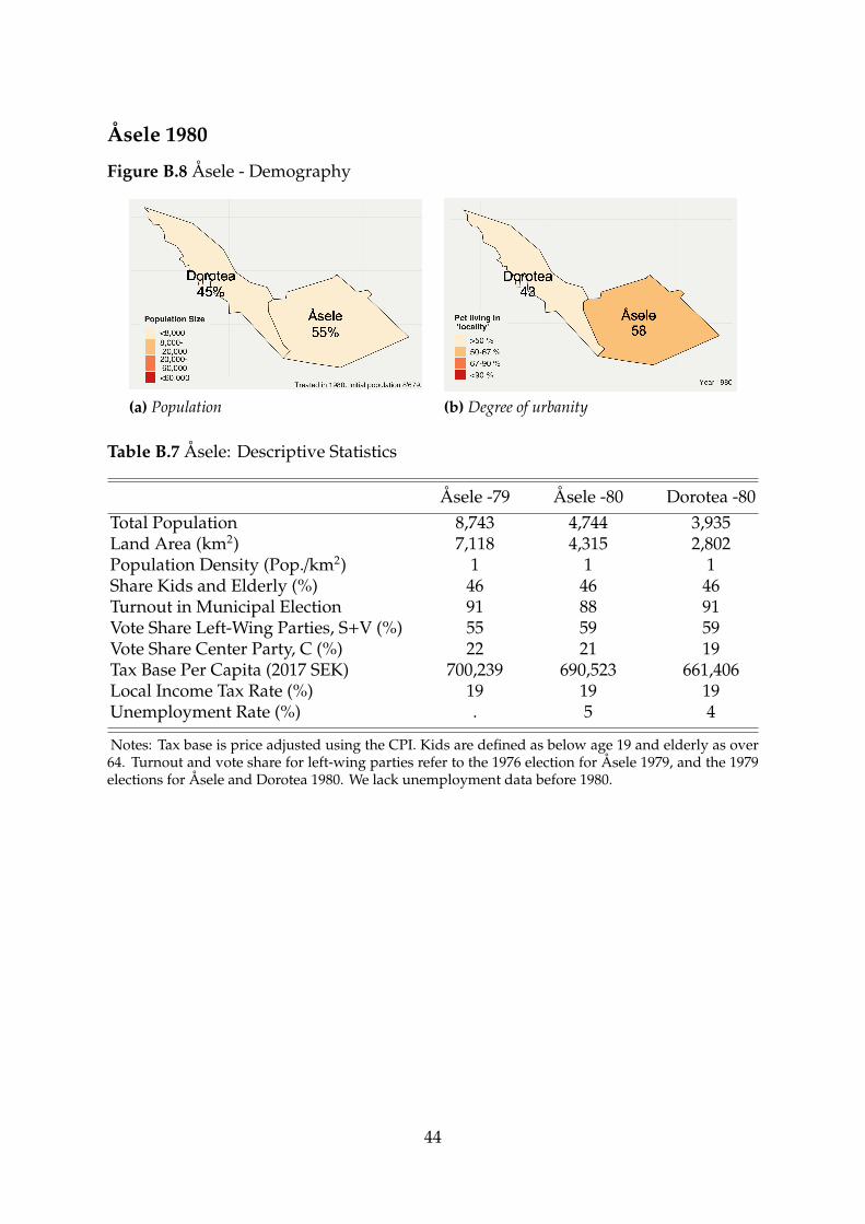
Åsele 1980
Figure B.8 Åsele - Demography
(a) Population (b) Degree of urbanity
Table B.7 Åsele: Descriptive Statistics
Åsele -79 Åsele -80 Dorotea -80Total Population 8,743 4,744 3,935Land Area (km2) 7,118 4,315 2,802Population Density (Pop./km2) 1 1 1Share Kids and Elderly (%) 46 46 46Turnout in Municipal Election 91 88 91Vote Share Left-Wing Parties, S+V (%) 55 59 59Vote Share Center Party, C (%) 22 21 19Tax Base Per Capita (2017 SEK) 700,239 690,523 661,406Local Income Tax Rate (%) 19 19 19Unemployment Rate (%) . 5 4
Notes: Tax base is price adjusted using the CPI. Kids are defined as below age 19 and elderly as over64. Turnout and vote share for left-wing parties refer to the 1976 election for Åsele 1979, and the 1979elections for Åsele and Dorotea 1980. We lack unemployment data before 1980.
44
Appendix C: Estimation and Implementation
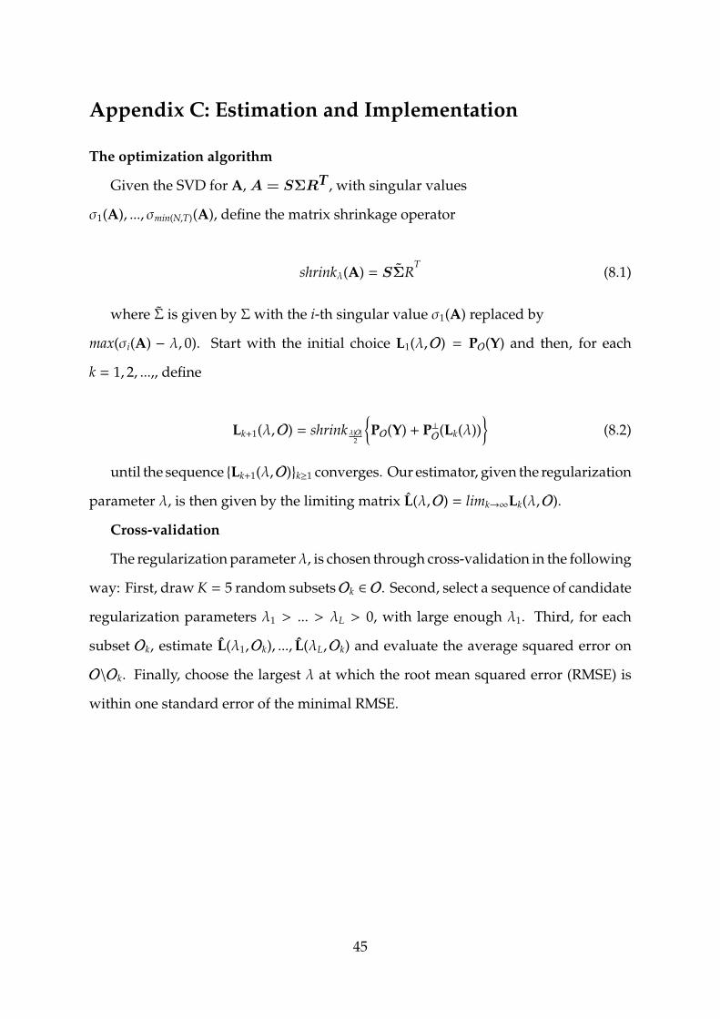
The optimization algorithm
Given the SVD for A, A = SΣRT , with singular values
σ1(A), ..., σmin(N,T)(A), define the matrix shrinkage operator
shrinkλ(A) = SΣRT
(8.1)
where Σ is given by Σ with the i-th singular value σ1(A) replaced by
max(σi(A) − λ, 0). Start with the initial choice L1(λ,O) = PO(Y) and then, for each
k = 1, 2, ...,, define
Lk+1(λ,O) = shrink λ|O|2
{PO(Y) + P⊥
O(Lk(λ))
}(8.2)
until the sequence {Lk+1(λ,O)}k≥1 converges. Our estimator, given the regularization
parameter λ, is then given by the limiting matrix L(λ,O) = limk→∞Lk(λ,O).
Cross-validation
The regularization parameterλ, is chosen through cross-validation in the following
way: First, draw K = 5 random subsetsOk ∈ O. Second, select a sequence of candidate
regularization parameters λ1 > ... > λL > 0, with large enough λ1. Third, for each
subset Ok, estimate L(λ1,Ok), ..., L(λL,Ok) and evaluate the average squared error on
O\Ok. Finally, choose the largest λ at which the root mean squared error (RMSE) is
within one standard error of the minimal RMSE.
45
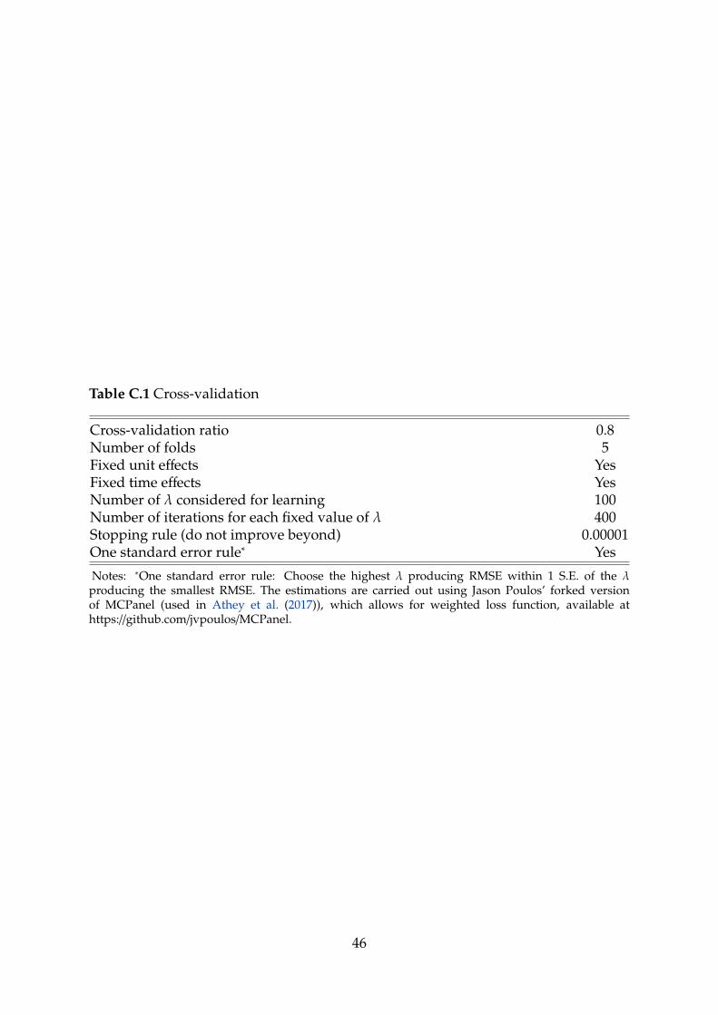
Table C.1 Cross-validation
Cross-validation ratio 0.8Number of folds 5Fixed unit effects YesFixed time effects YesNumber of λ considered for learning 100Number of iterations for each fixed value of λ 400Stopping rule (do not improve beyond) 0.00001One standard error rule∗ Yes
Notes: ∗One standard error rule: Choose the highest λ producing RMSE within 1 S.E. of the λproducing the smallest RMSE. The estimations are carried out using Jason Poulos’ forked versionof MCPanel (used in Athey et al. (2017)), which allows for weighted loss function, available athttps://github.com/jvpoulos/MCPanel.
46
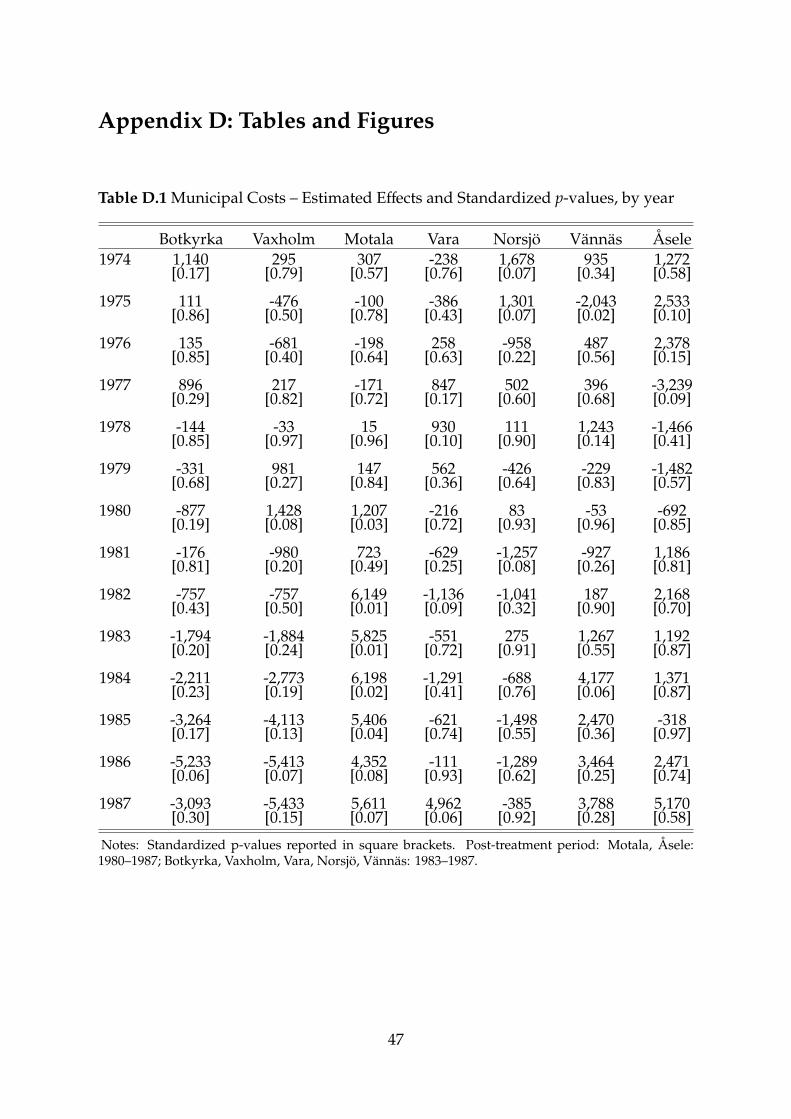
Appendix D: Tables and Figures
Table D.1 Municipal Costs – Estimated Effects and Standardized p-values, by year
Botkyrka Vaxholm Motala Vara Norsjö Vännäs Åsele1974 1,140 295 307 -238 1,678 935 1,272
[0.17] [0.79] [0.57] [0.76] [0.07] [0.34] [0.58]
1975 111 -476 -100 -386 1,301 -2,043 2,533[0.86] [0.50] [0.78] [0.43] [0.07] [0.02] [0.10]
1976 135 -681 -198 258 -958 487 2,378[0.85] [0.40] [0.64] [0.63] [0.22] [0.56] [0.15]
1977 896 217 -171 847 502 396 -3,239[0.29] [0.82] [0.72] [0.17] [0.60] [0.68] [0.09]
1978 -144 -33 15 930 111 1,243 -1,466[0.85] [0.97] [0.96] [0.10] [0.90] [0.14] [0.41]
1979 -331 981 147 562 -426 -229 -1,482[0.68] [0.27] [0.84] [0.36] [0.64] [0.83] [0.57]
1980 -877 1,428 1,207 -216 83 -53 -692[0.19] [0.08] [0.03] [0.72] [0.93] [0.96] [0.85]
1981 -176 -980 723 -629 -1,257 -927 1,186[0.81] [0.20] [0.49] [0.25] [0.08] [0.26] [0.81]
1982 -757 -757 6,149 -1,136 -1,041 187 2,168[0.43] [0.50] [0.01] [0.09] [0.32] [0.90] [0.70]
1983 -1,794 -1,884 5,825 -551 275 1,267 1,192[0.20] [0.24] [0.01] [0.72] [0.91] [0.55] [0.87]
1984 -2,211 -2,773 6,198 -1,291 -688 4,177 1,371[0.23] [0.19] [0.02] [0.41] [0.76] [0.06] [0.87]
1985 -3,264 -4,113 5,406 -621 -1,498 2,470 -318[0.17] [0.13] [0.04] [0.74] [0.55] [0.36] [0.97]
1986 -5,233 -5,413 4,352 -111 -1,289 3,464 2,471[0.06] [0.07] [0.08] [0.93] [0.62] [0.25] [0.74]
1987 -3,093 -5,433 5,611 4,962 -385 3,788 5,170[0.30] [0.15] [0.07] [0.06] [0.92] [0.28] [0.58]
Notes: Standardized p-values reported in square brackets. Post-treatment period: Motala, Åsele:1980–1987; Botkyrka, Vaxholm, Vara, Norsjö, Vännäs: 1983–1987.
47
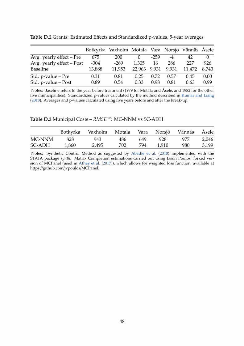
Table D.2 Grants: Estimated Effects and Standardized p-values, 5-year averages
Botkyrka Vaxholm Motala Vara Norsjö Vännäs ÅseleAvg. yearly effect – Pre 675 200 0 -259 -4 42 0Avg. yearly effect – Post -304 -269 1,305 16 286 227 926Baseline 13,888 11,953 22,963 9,931 9,931 11,472 8,743Std. p-value – Pre 0.31 0.81 0.25 0.72 0.57 0.45 0.00Std. p-value – Post 0.89 0.54 0.33 0.98 0.81 0.63 0.99
Notes: Baseline refers to the year before treatment (1979 for Motala and Åsele, and 1982 for the otherfive municipalities). Standardized p-values calculated by the method described in Kumar and Liang(2018). Averages and p-values calculated using five years before and after the break-up.
Table D.3 Municipal Costs – RMSEpre: MC-NNM vs SC-ADH
Botkyrka Vaxholm Motala Vara Norsjö Vännäs ÅseleMC-NNM 828 943 486 649 928 977 2,046SC-ADH 1,860 2,495 702 794 1,910 980 3,199
Notes: Synthetic Control Method as suggested by Abadie et al. (2010) implemented with theSTATA package synth. Matrix Completion estimations carried out using Jason Poulos’ forked ver-sion of MCPanel (used in Athey et al. (2017)), which allows for weighted loss function, available athttps://github.com/jvpoulos/MCPanel.
48
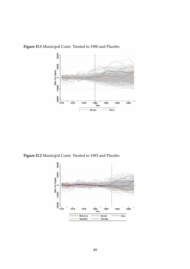
Figure D.1 Municipal Costs: Treated in 1980 and Placebo
Figure D.2 Municipal Costs: Treated in 1983 and Placebo
49
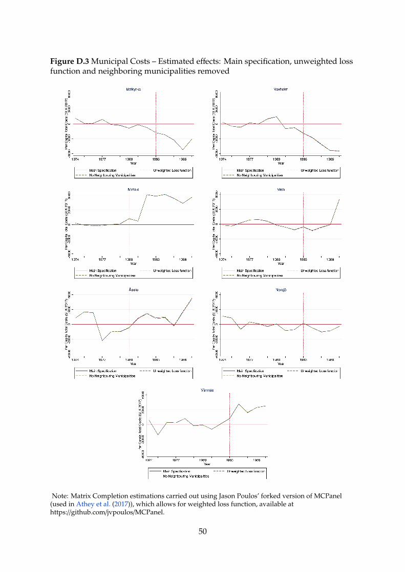
Figure D.3 Municipal Costs – Estimated effects: Main specification, unweighted lossfunction and neighboring municipalities removed
Note: Matrix Completion estimations carried out using Jason Poulos’ forked version of MCPanel(used in Athey et al. (2017)), which allows for weighted loss function, available athttps://github.com/jvpoulos/MCPanel.
50
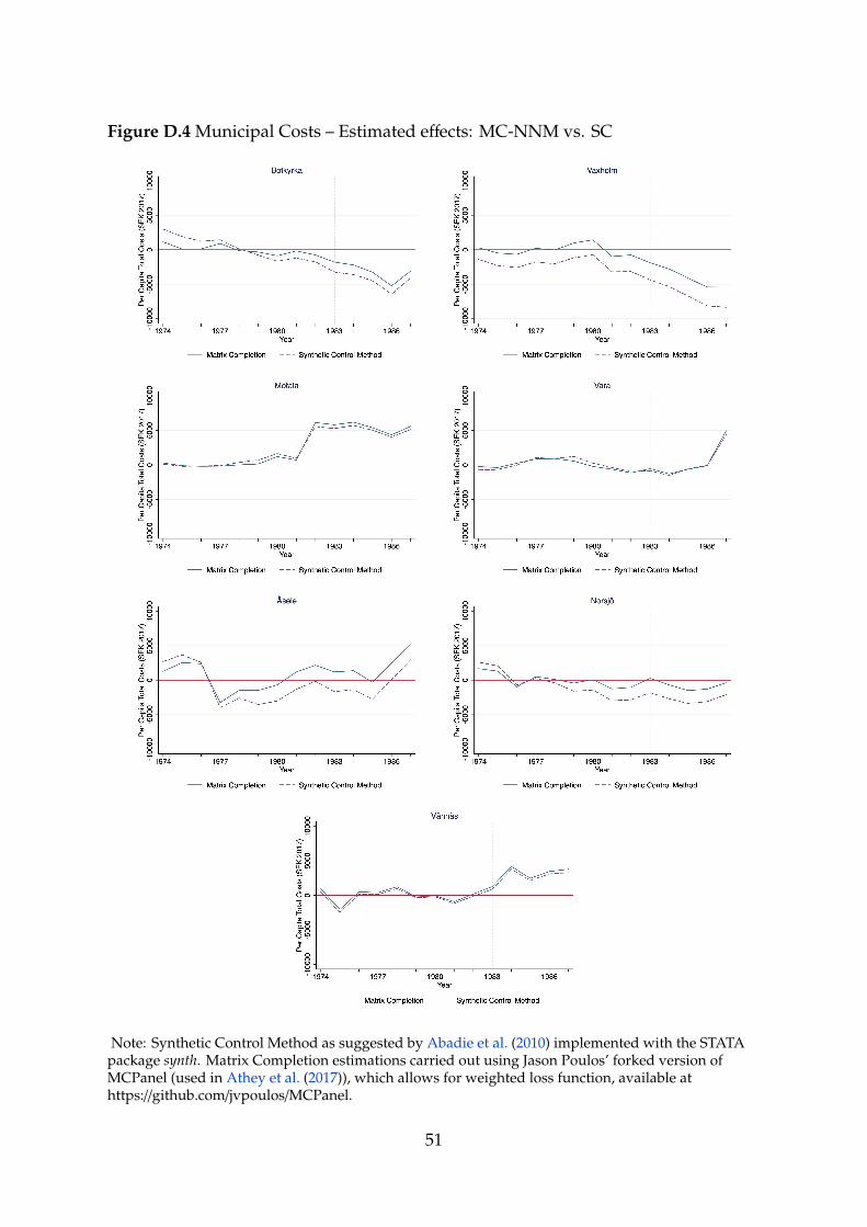
Figure D.4 Municipal Costs – Estimated effects: MC-NNM vs. SC
Note: Synthetic Control Method as suggested by Abadie et al. (2010) implemented with the STATApackage synth. Matrix Completion estimations carried out using Jason Poulos’ forked version ofMCPanel (used in Athey et al. (2017)), which allows for weighted loss function, available athttps://github.com/jvpoulos/MCPanel.
51
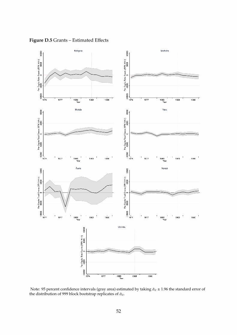
Figure D.5 Grants – Estimated Effects
Note: 95 percent confidence intervals (gray area) estimated by taking αit ± 1.96 the standard error ofthe distribution of 999 block bootstrap replicates of αit.
52