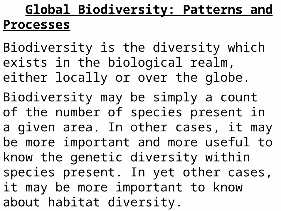
Global Biodiversity: Patterns and Processes

Biodiversity is the diversity which exists in the biological realm, either locally or over the globe.

Biodiversity may be simply a count of the number of species present in a given area. In other cases, it may be more important and more useful to know the genetic diversity within species present. In yet other cases, it may be more important to know about habitat diversity.

Numbers from the UN Environmental Program book suggest we have named and catalogued ~1.75 million species. The UN adopted an estimate of 13.6 million species total alive on earth.

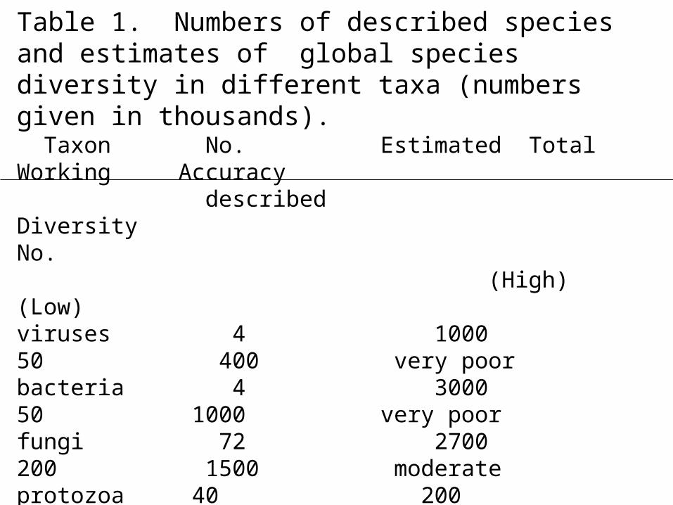
Table 1.  Numbers of described species and estimates of global species diversity in different taxa (numbers given in thousands).  Taxon       No.          Estimated Total Working Accuracy described         Diversity            No.                          (High)      (Low)viruses        4          1000         50         400     very poorbacteria       4          3000         50        1000     very poor fungi          72         2700        200        1500     moderateprotozoa     40         200          60         200     very poor algae          40         1000        150         400     very poor plants        270         500        300         320     goodnematodes  25         1000       100         400     poorarthropods  crustacea 40          200          75         150     moderate arachnids 75          1000      300      750    moderate  insects    950         100000      2000        8000      moderate

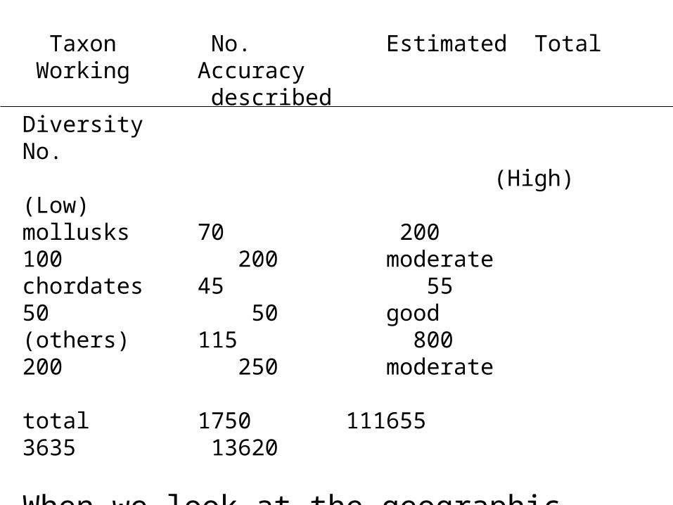
  Taxon       No.          Estimated Total Working Accuracy described         Diversity            No.                          (High)      (Low)mollusks     70          200          100          200     moderatechordates    45          55          50         50      good(others)     115         800          200          250     moderate

total        1750       111655        3635       13620

When we look at the geographic distribution of diversity, our knowledge is most limited in the regions which are believed to contain the highest diversity of species.

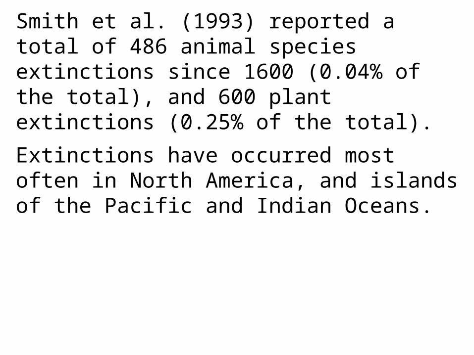
Smith et al. (1993) reported a total of 486 animal species extinctions since 1600 (0.04% of the total), and 600 plant extinctions (0.25% of the total).

Extinctions have occurred most often in North America, and islands of the Pacific and Indian Oceans.

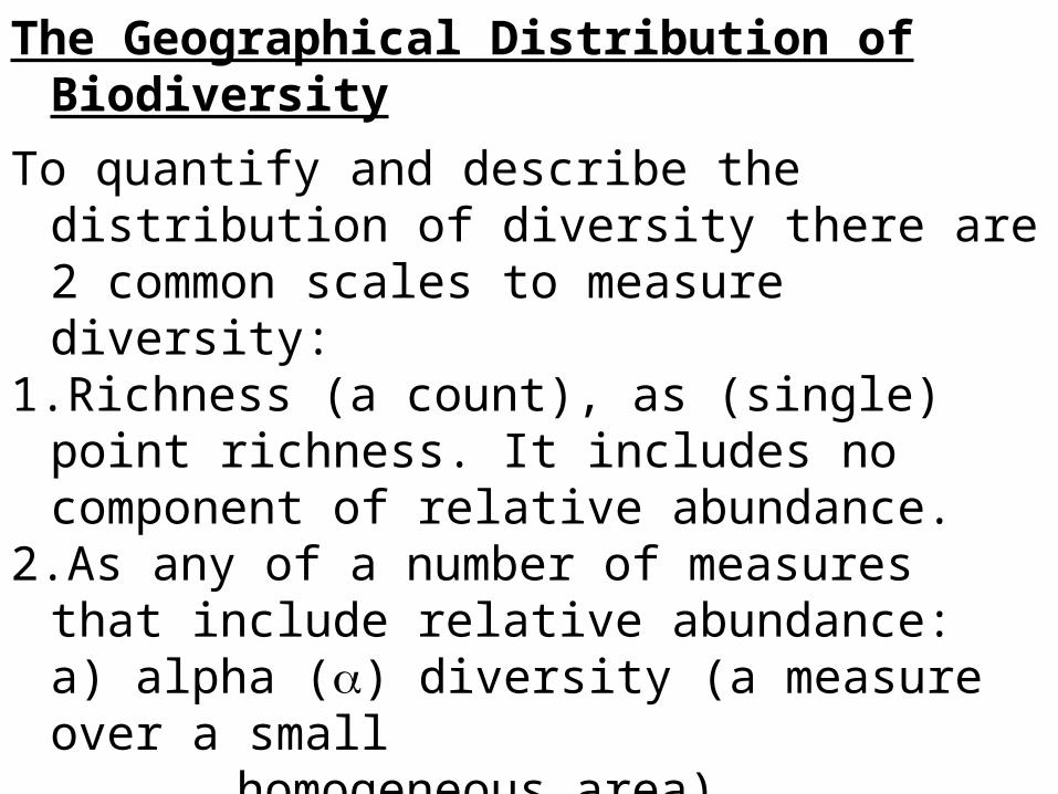
The Geographical Distribution of Biodiversity

To quantify and describe the distribution of diversity there are 2 common scales to measure diversity:

1.Richness (a count), as (single) point richness. It includes no component of relative abundance.

2.As any of a number of measures that include relative abundance:a) alpha () diversity (a measure over a small

homogeneous area), b) beta () diversity (rate of change of species composition over a habitat gradient, and

c) gamma () diversity, which looks at similar changes over entire landscapes.

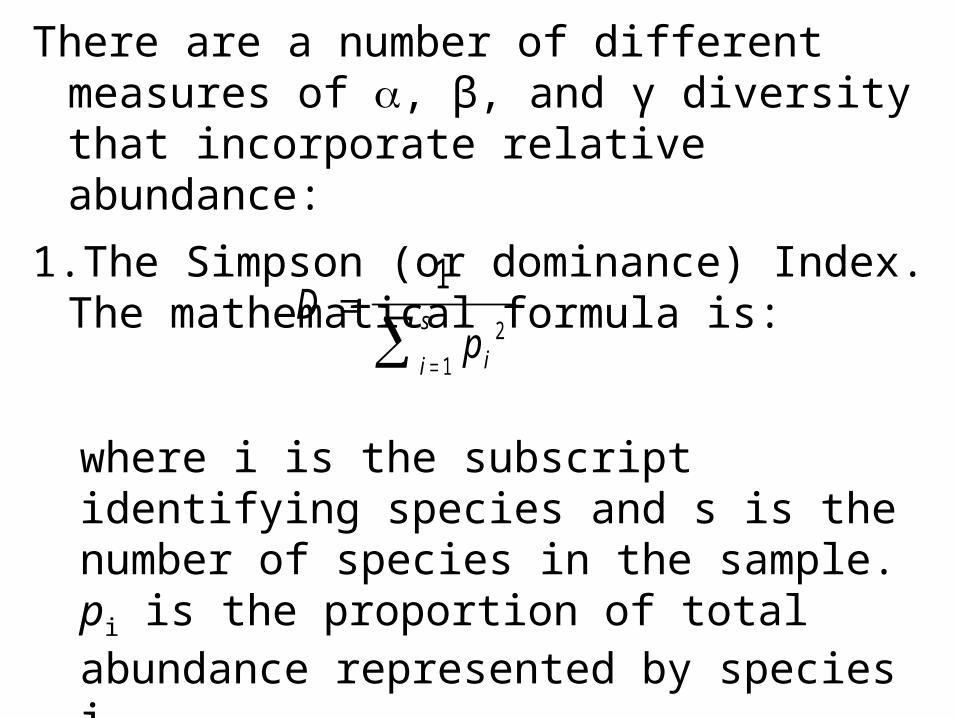
There are a number of different measures of , β, and γ diversity that incorporate relative abundance:

1.The Simpson (or dominance) Index. The mathematical formula is:

Dp ii

s1

2

1

where i is the subscript identifying species and s is the number of species in the sample. pi is the proportion of total abundance represented by species i.

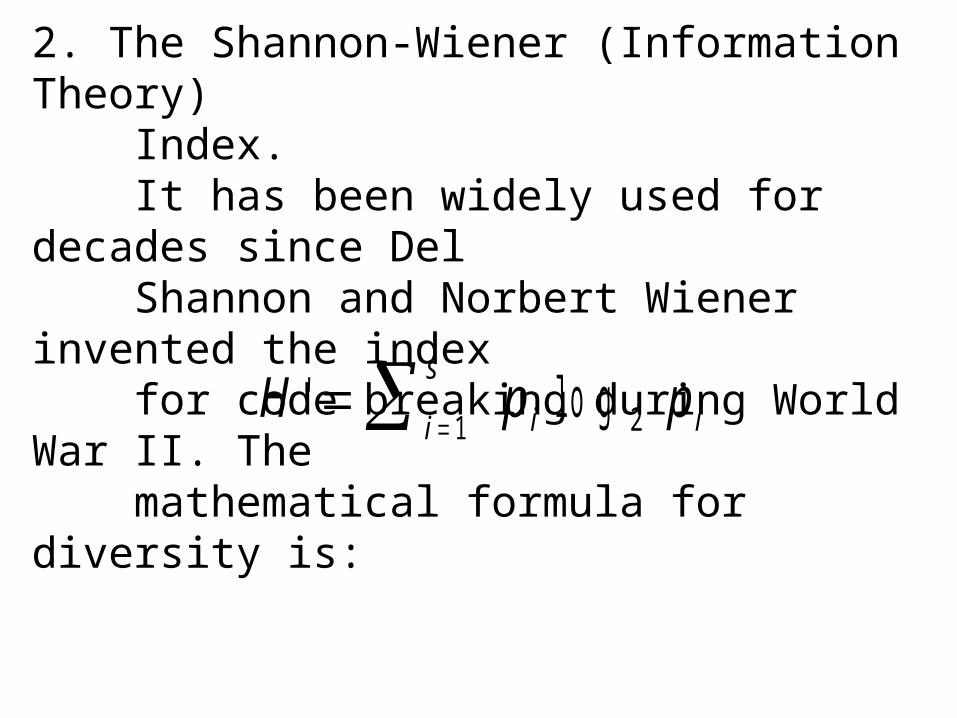
2. The Shannon-Wiener (Information Theory) Index.   It has been widely used for decades since Del Shannon and Norbert Wiener invented the index for code breaking during World War II. The mathematical formula for diversity is:

In this case relative abundance is assessed as evenness, and is based on the ratio of the observed diversity index to the one which would have been found had all species been equally abundant.

H p pi

s

i i' lo g 1 2

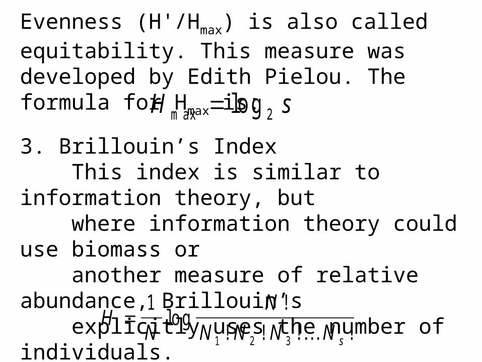
Evenness (H'/Hmax) is also called equitability. This measure was developed by Edith Pielou. The formula for Hmax is:

H sm ax lo g 2

3. Brillouin’s Index This index is similar to information theory, but where information theory could use biomass or another measure of relative abundance, Brillouin’s explicitly uses the number of individuals. Mathematically:

HN

N

N N N N s

1

1 2 3

lo g!

! ! !. . . !

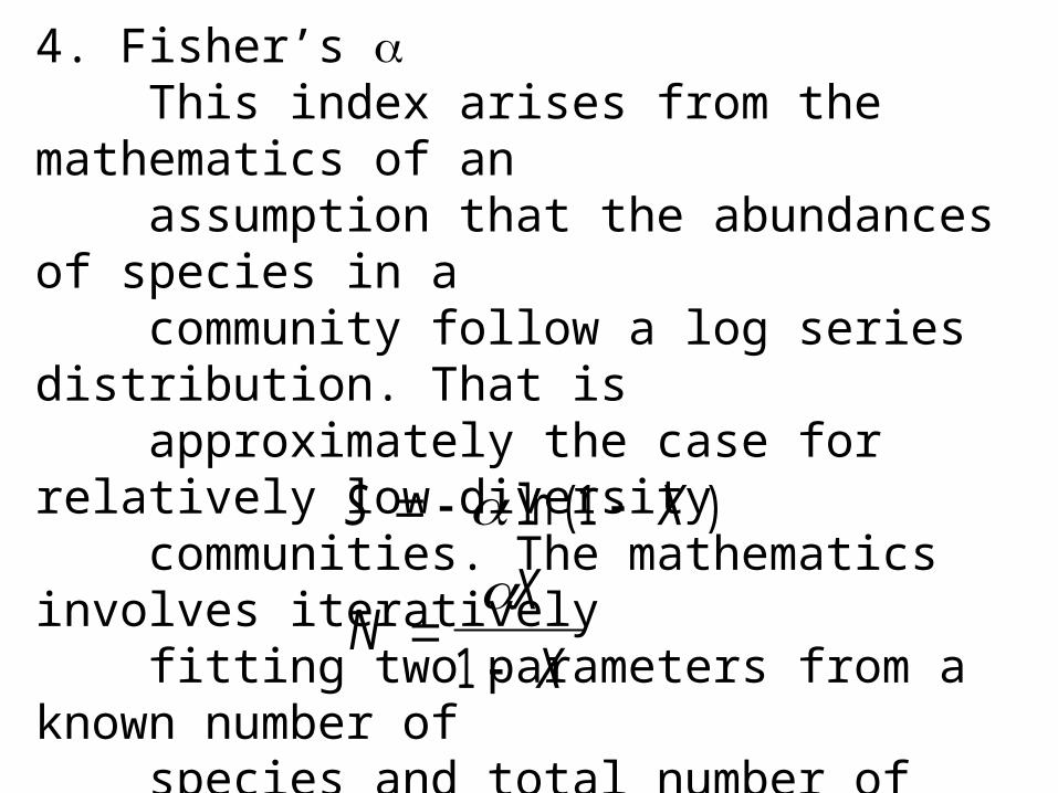
4. Fisher’s This index arises from the mathematics of an assumption that the abundances of species in a community follow a log series distribution. That is approximately the case for relatively low diversity communities. The mathematics involves iteratively fitting two parameters from a known number of species and total number of individuals…S X

NX

X

ln ( )1

1

Geographic Patterns of Diversity - Plots of Physical Variables

Geographical survey can be developed at two levels:

1. Classical division of the various biomes along gradients in basic physical variables. The nicer the climate is, the more diverse the community of

species should be.

An example: We would expect low diversity in polar desert communities, and the diversity is very low. There is little precipitation and a very low rate of decomposition, so that nutrients are not readily available and soils are poorly developed.

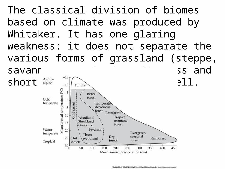
The classical division of biomes based on climate was produced by Whitaker. It has one glaring weakness: it does not separate the various forms of grassland (steppe, savanna, grassland, tall grass and short grass prairies) very well.

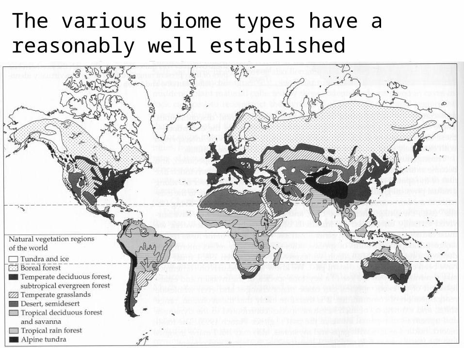
The various biome types have a reasonably well established geographical distribution over the globe.

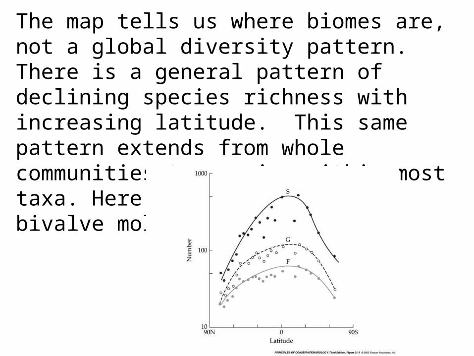
The map tells us where biomes are, not a global diversity pattern. There is a general pattern of declining species richness with increasing latitude. This same pattern extends from whole communities to species within most taxa. Here is the pattern for bivalve mollusks:

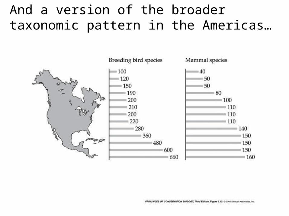
And a version of the broader taxonomic pattern in the Americas…

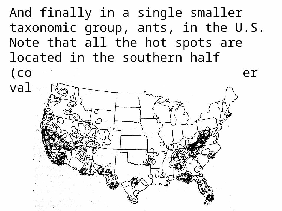
And finally in a single smaller taxonomic group, ants, in the U.S. Note that all the hot spots are located in the southern half (concentric rings indicate higher values ‘in the center’.

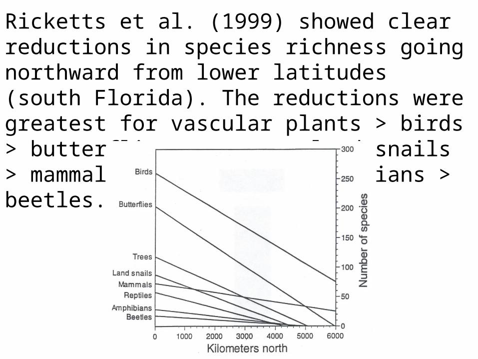
Ricketts et al. (1999) showed clear reductions in species richness going northward from lower latitudes (south Florida). The reductions were greatest for vascular plants > birds > butterflies > trees > land snails > mammals > reptiles > amphibians > beetles.

The general pattern is one described as latitudinal gradients in diversity.

We can dismiss one hypothesis (as obvious) early. There are more species at lower latitudes because there are more habitat types. Why?

Adiabatic lapse means that at higher elevations in tropical areas the cooler climates of temperate areas are reproduced, and at extremely high elevations arctic conditions may occur. The converse is impossible; there is no means for tropical conditions to be reproduced in temperate latitudes. So inevitably, the overall habitat diversity of the tropics is greater than that at higher latitudes.

However, the real question is why there is a higher within habitat diversity at lower latitudes?

Pianka (1994) provided a set of hypotheses and explanations for these patterns.

1.Evolutionary time - diversity should increase with the age of a community. It assumes that temperate and more extreme latitudes remain impoverished as a result of the cycles of Pleistocene glaciation. Evolutionary response to the restoration of interglacial climates is still in progress.

There are problems with this hypothesis. Tropical communities were affected by recent glaciations.

The cycles of Pleistocene glaciation are argued to be one of the most important forces in explaining tropical forest diversity.

During each cycle of glaciation, continuous bands of tropical forest became fragmented. Species differentiation occurred in each of these fragments, potentially during each cycle, so that what began as a single tropical forest species at the outset of the Pleistocene could have become 8 different species (4 cycles of glaciation: 12 4 8) times the number of isolated fragments, which number at least 6-8.

The other problem is that the hypothesis is founded largely on a northern hemisphere view.

Because land area is smaller at temperate latitudes in the southern hemisphere, there was little Pleistocene glaciation south of the equator. Should temperate communities in the south temperate zone be considered as 'young' as those at similar latitudes north of the equator? (They are about equally impoverished.)

A separate issue is repeated cycles of mass extinction and re-diversification.

On average, diversity has increased over the geological time scale, but the increase has not been smooth and uniform. There have been a number of episodes of mass extinction in which a significant fraction of living taxa have disappeared over fairly short times.

The rate of diversification following each mass extinction was much higher than at other times, in each case due to the availability of resources and niche space.

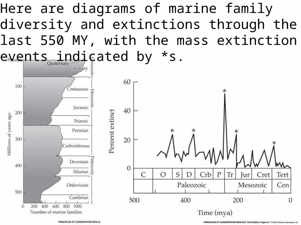
Here are diagrams of marine family diversity and extinctions through the last 550 MY, with the mass extinction events indicated by *s.

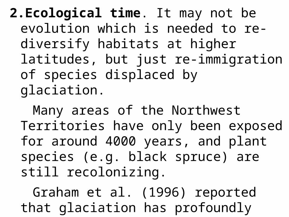
2.Ecological time. It may not be evolution which is needed to re-diversify habitats at higher latitudes, but just re-immigration of species displaced by glaciation.

Many areas of the Northwest Territories have only been exposed for around 4000 years, and plant species (e.g. black spruce) are still recolonizing.

Graham et al. (1996) reported that glaciation has profoundly affected North American mammal distributions. During Pleistocene glaciation, species like muskox and caribou extended down into this area (and farther south).    

3. Climatic stability. A stable climate is one which changes little over time, both seasonally and from year to year. A species living in a stable climate can evolve specialized adaptations to the specific climate. One which lives in an unstable or unpredictable climate must have broad tolerance limits, and, logically, broad niches. That leaves niche space for fewer species.

4. Climatic predictability. If a climate is highly predictable, the species can evolve life history adaptations which reflect climatic cycles, for example winter or drought dormancy.

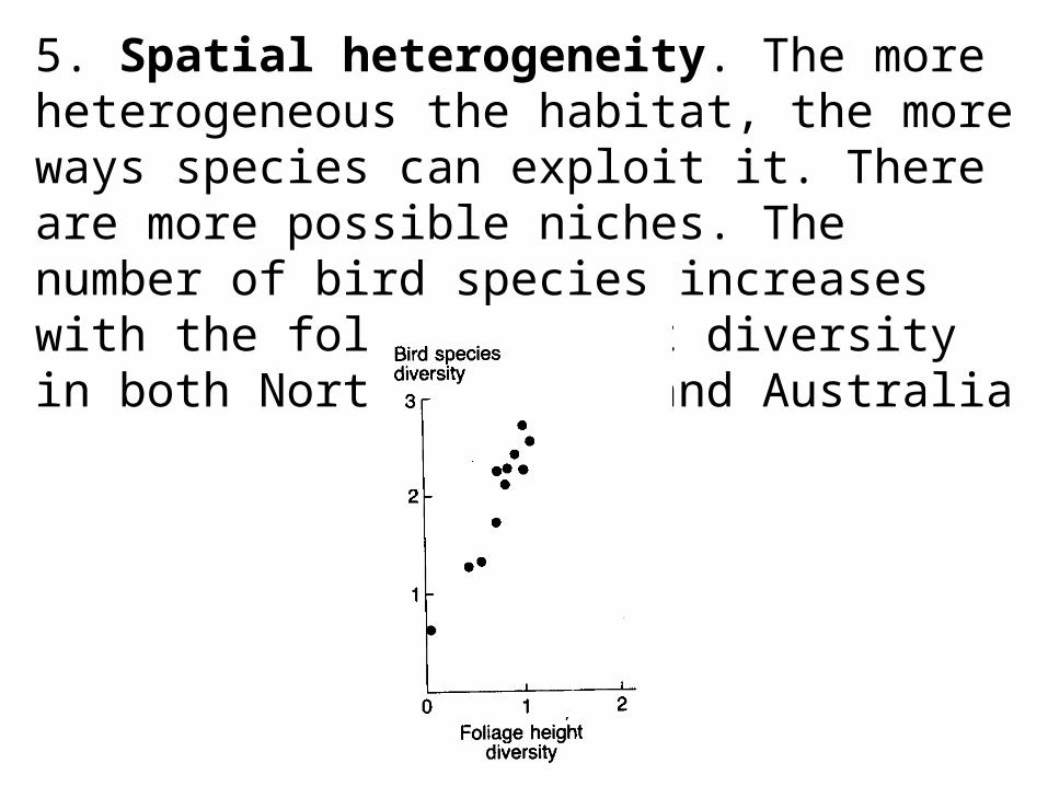
5. Spatial heterogeneity. The more heterogeneous the habitat, the more ways species can exploit it. There are more possible niches. The number of bird species increases with the foliage height diversity in both North America and Australia

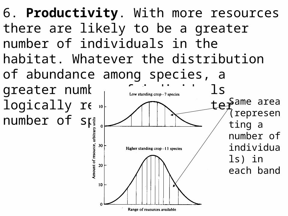
6. Productivity. With more resources there are likely to be a greater number of individuals in the habitat. Whatever the distribution of abundance among species, a greater number of individuals logically results in a greater number of species.

Same area (representing a number of individuals) in each band

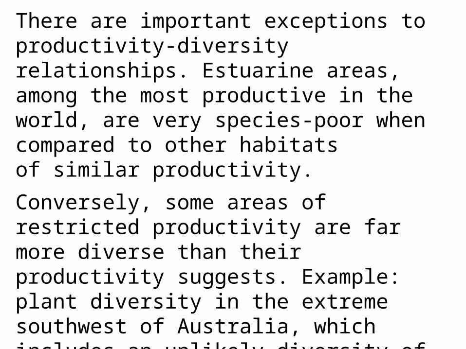
There are important exceptions to productivity-diversity relationships. Estuarine areas, among the most productive in the world, are very species-poor when compared to other habitats of similar productivity.

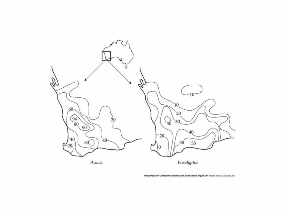
Conversely, some areas of restricted productivity are far more diverse than their productivity suggests. Example: plant diversity in the extreme southwest of Australia, which includes an unlikely diversity of Eucalyptus and Acacia species in small areas

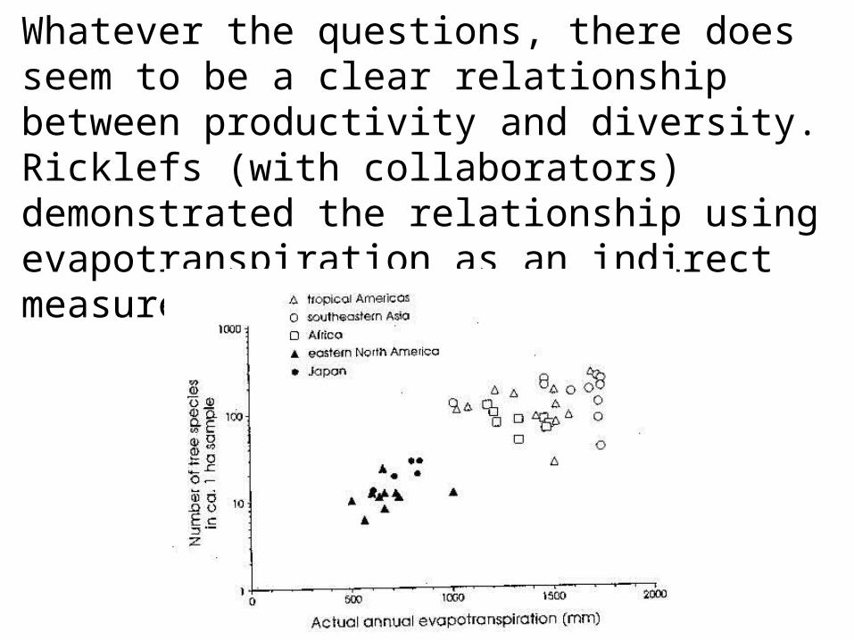
Whatever the questions, there does seem to be a clear relationship between productivity and diversity. Ricklefs (with collaborators) demonstrated the relationship using evapotranspiration as an indirect measure of photosynthesis…

7. Stability of primary production. Extend the arguments about climatic stability to stability in the energy supply available to food chains and webs. More species can be supported with a finer division of resources if the amount of available resource is predictable.

8. Competition. If competition is intense, then selection produces populations which have differentiated niches. Specialization which results from competition leaves narrower niches and greater diversity.

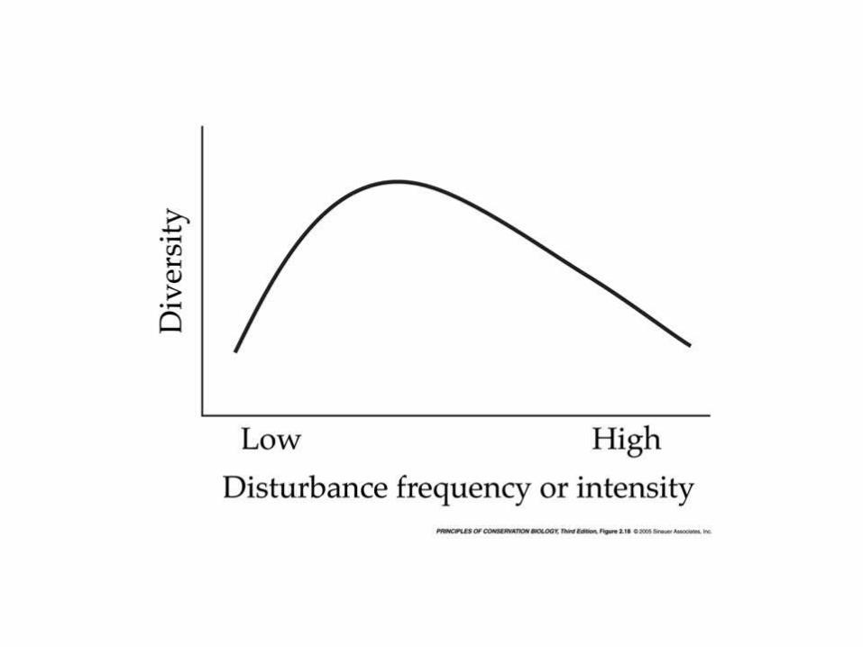
9. Disturbance. This is essentially the antithesis of the competition hypothesis. Disturbances reduce the intensity and effect of competition, and reduce the diversity. In undisturbed communities competitive dominants occupy most of the space in the community. In very frequently disturbed communities pioneer (weedy) species dominate.

However, intermediate frequency and/or intensity of disturbance can clear space in a community, and allow diversity to increase.

This idea is called the intermediate disturbance hypothesis (Connell 1978).

10.Predation. Predation reduces the population size of dominant species. That rarefaction reduces the intensity of competition among prey, and can permit the coexistence of species which would otherwise suffer competitive exclusion. When the difference in diversity in the presence and absence of a predator is large, we call it a keystone species.

Whether there is a latitudinal gradient to be expected in predator effects is open to question. Whether diversity can be affected locally is not in question.

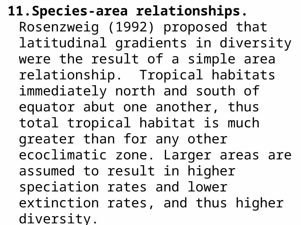
11.Species-area relationships. Rosenzweig (1992) proposed that latitudinal gradients in diversity were the result of a simple area relationship.  Tropical habitats immediately north and south of equator abut one another, thus total tropical habitat is much greater than for any other ecoclimatic zone. Larger areas are assumed to result in higher speciation rates and lower extinction rates, and thus higher diversity.

Chown and Gaster (2000) criticized this hypothesis with three lines of evidence:

a. there is no relationship between species’ range size and habitat area available in the biome; 

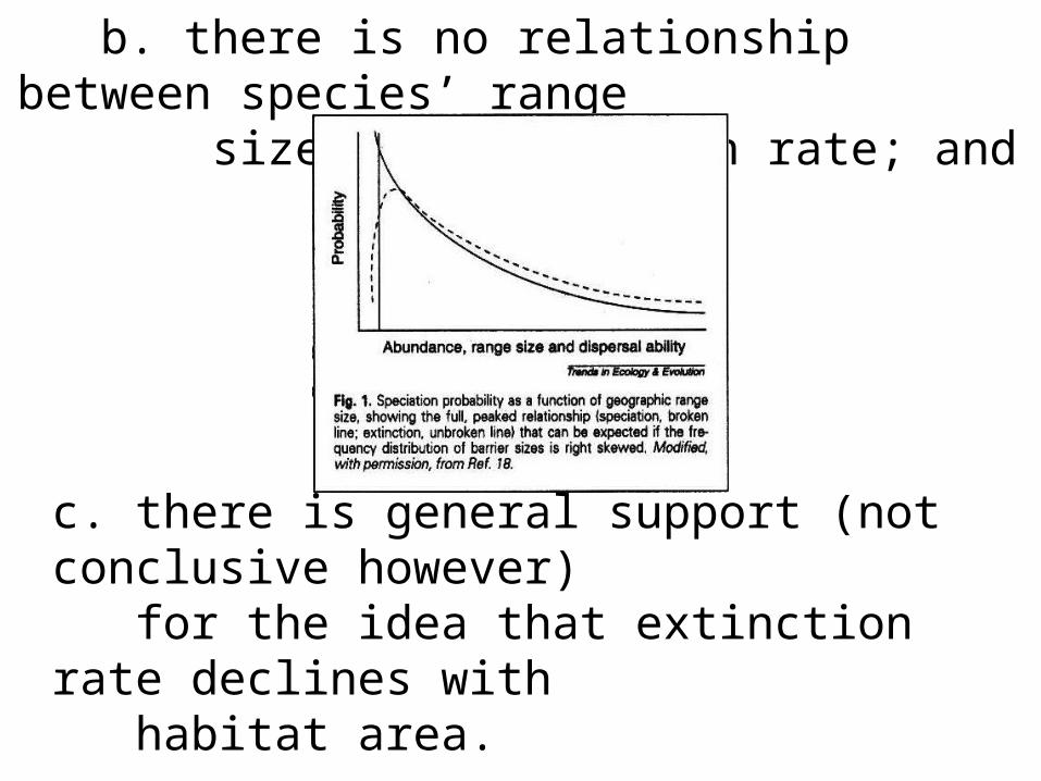
b. there is no relationship between species’ range size and speciation rate; and

c. there is general support (not conclusive however) for the idea that extinction rate declines with habitat area.

a, b and c should all be true to support Rosenzweig’s hypothesis.

12.Evolutionary Speed. Higher temperatures in tropics fosters an elevated speciation rate since generation times are lower.

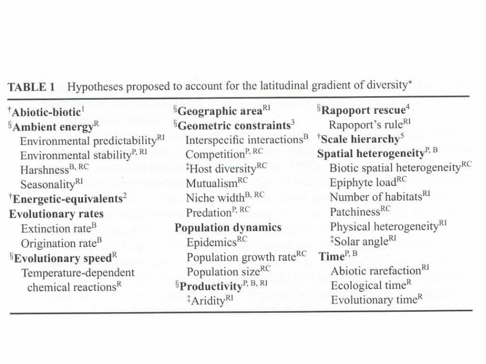
Many more hypotheses have been proposed, and no single answer alone is likely to be correct. This is a recent table (Willig 2003) of the many suggested hypotheses:

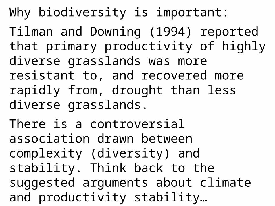
Why biodiversity is important:

Tilman and Downing (1994) reported that primary productivity of highly diverse grasslands was more resistant to, and recovered more rapidly from, drought than less diverse grasslands.

There is a controversial association drawn between complexity (diversity) and stability. Think back to the suggested arguments about climate and productivity stability…

When we consider the potential impact of global change, high biodiversity may be a protective factor.

Finally, a little supplementary information about known causes of the mass extinctions:

a) Perhaps the leading explanation is the comet (or asteroid) impact (or Alvarez) hypothesis. Impact of a small comet or asteroid would create a dust cloud far larger than would be created by any known nuclear weapon. The Cretaceous mass extinction is associated with the deposition of a layer rich in iridium, which is more common in comets and asteroids than the surface of earth. That may mean dust settled from a collision. The likely site of impact (the Chicxulub crater) of an asteroid of about 17km diameter has been found off the Yucatan Peninsula of Mexico.

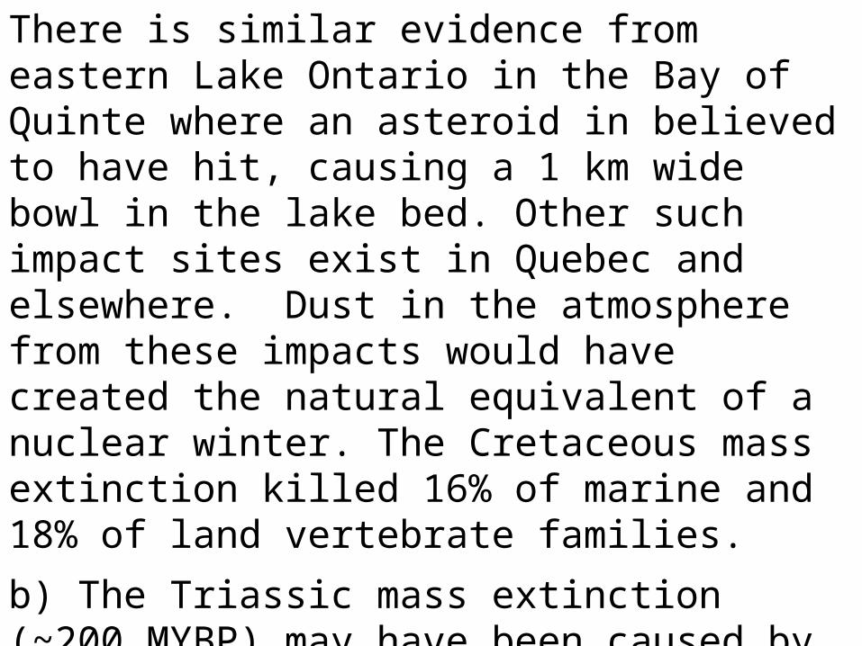
There is similar evidence from eastern Lake Ontario in the Bay of Quinte where an asteroid in believed to have hit, causing a 1 km wide bowl in the lake bed. Other such impact sites exist in Quebec and elsewhere. Dust in the atmosphere from these impacts would have created the natural equivalent of a nuclear winter. The Cretaceous mass extinction killed 16% of marine and 18% of land vertebrate families.

b) The Triassic mass extinction (~200 MYBP) may have been caused by massive mid-Atlantic magma/ volcanic activity that rifted Africa from South America. It would have caused enormous global warming.

The toll of this warming: 22% of marine families, and an unclear number of terrestrial families.

c. The cause of the Permian mass extinction is not clear. It may have been caused by an asteroid collision, or by vulcanism arising from such a collision. It occurred ~251 MYBP. It was the most devastating extinction, killing 95% of all species, including 70% of terrestrial species of all kinds.

d. The Devonian mass extinction (364 MYBP) is unexplained. It resulted in the loss of 22% of marine families and 57% of marine genera.

e. An emerging hypothesis suggests that the end-of-Ordovician extinction (~440 MYBP), which wiped out about 66% of species 440 million years ago, could have been caused by ultraviolet radiation from the sun after gamma rays destroyed the Earth's ozone layer. It’s been suggested that a supernova exploded near the Earth, destroying the chemistry of the atmosphere and allowing the sun's ultraviolet rays to cook fragile, unprotected life forms. These ideas were suggested in 2003 by Adrian Melott, a University of Kansas astronomer.

Fossil records for the Ordovician extinction show an abrupt disappearance of two-thirds of all species, while other records show an ice age that lasted more than a half million years started at the same time. Sea level first fell with glaciation, then rose with glacial melting. Melott said a gamma ray burst striking the Earth would break up molecules in the stratosphere, causing the formation of nitrous oxide and other chemicals that would destroy the ozone layer and shroud the planet in a brown smog.

The losses: 25% of marine families and 60% of marine genera.

ReferencesBrown, J. and M.V. Lomolino 1998. Biogeography.  Chapter 5.

Cameron, T. 2002. 2002: the year of the ‘diversity-ecosystem function’ debate. Trends in Ecology & Evolution 17:495-496.

Chadwick-Furman, N.E. 1996. Reef coral diversity and global climate change. Global Change Biology 2: 559-568.

Chown, S.L. and K.J. Gaston. 2000. Areas, cradles and museums: the latitudinal gradient in species richness.  Trends in Ecology & Evolution 15:311-315.

Connell, J.H. 1978. Diversity in tropical rain forests and coral reefs. Science 199:1302-1310.

Graham et al. 1996. Spatial response of mammals to late Quaternary environmental fluctuations. Science 272:1601-1606.

Heywood, V.H. (ed.) 1995. Global Biodiversity Assessment. UNEP. Cambridge Univ. Press, Cambridge.

Johnson, K.H. et al. 1996. Biodiversity and the productivity and stability of ecosystems. Trends in Ecology & Evolution 11:372-377.

Kruger, F.J. and H.C. Taylor. 1979. Plant species diversity in Cape fynbos: Gamma and delta diversity. Vegetatio 41:85-93.

Latham , R.E. and R.E. Ricklefs. 1993. Global patterns of tree species richness in moist forests: energy-diversity theory does not account for variation in species richness. Oikos 67:325-333.

Pianka, E.R. 1994. Evolutionary Ecology.  5th Ed. Harper & Row, N.Y.

Price, A.R.G. 2002. Simultaneous ‘hotspots’ and ‘coldspots’ of marine biodiversity and implications for global conservation. Marine Ecology Progress Series 241:23-27.

Recher , H.F. 1969.  Bird species diversity and habitat diversity in Australia and North America. American Naturalist 103:75-80.

Rice B. and M. Westoby. 1983. Species richness at tenth-hectare scale in Australian vegetation compared to other continents. Vegetatio 52:129-140.

Ricketts, T.H., E. Dinerstein, D.M. Olson and C. Loucks. 1999. Who’s where in North America? Bioscience 49: 369-381.

Smith, F.D.M. et al. 1993. How much do we know about the current extinction rate?  Trends in Ecology & Evolution 8:375-378.

Willig, M., D. Kaufman, and R. Stevens. 2003. Latitudinal gradients of biodiversity: Pattern, process, scale, and synthesis. Annual Review of Ecology and Systematics 34: 273-309.

Tilman, D., and J.A. Downing. 1994. Biodiversity and stability in grasslands. Nature 367:363-366.