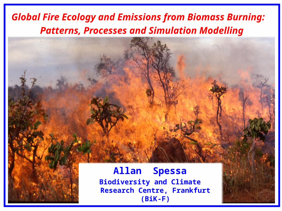
Global Fire Ecology and Emissions from Biomass Burning:

Patterns, Processes and Simulation Modelling

Allan SpessaBiodiversity and Climate Research Centre,

Frankfurt (BiK-F)

Talk Overview

1. Why is fire important in the earth system?

2. An overview of comtemporary fire patterns (ca. last 100 years).

3. Why simulate fire and emissions from biomass burning?

4. Modelling fire-vegetation interactions within the earth system.

Introducing the dynamic fire model SPITFIRE (Spread and Intensity

of Fires and Emissions), and the dynamic vegetation models ED

(Ecosystem Demography) and LPJ (Lund Potsdam Jena).

5. Model validation and data assimilation. Introduction to EO data.

6. Tropical peat fires. Deforestation-fire-climate interactions.

7. Simulating future fire- priorities and challenges?

Why is Fire Important in the Earth System I ?

1. Atmosphere forcing, atmospheric chemistry, and land-atmosphere

feedbacks

Global warming: Fire greenhouse gases CO2, CO, CH4 etc absorb thermal infrared

radiation. On average, about 3 Pg of carbon into the atmosphere per annum, and 0.6 PgC

from peat and deforestation fires. Much higher during drought events e.g. El Niño.

Global cooling: Fires aerosols scattering and absorption of incoming solar radiation.

Clouds: Smoke and haze can reduce rain droplet formation.

Burnt areas are darker (lower albedo) increase in radiation absorbed increase

convective activity.

Black carbon from boreal forest fires falling on snow/ice, thereby reducing its reflective

capacity.

Why is Fire Important in the Earth System II & III?

2. Plant reproduction & survival

Hot fires kill grasses and trees.

However, many plant species need intense fires to initiate germination and reproduce.

Consequences for ecological succession, land cover and carbon.

3. Carbon fluxes and biogeochemistry

Increase fire frequency more grass and fewer trees i.e. less carbon; & vice-versa.

Increase fire frequency decrease soil Nitrogen (volitisation and consumption of litter).

Peat is normally a below-ground carbon sink. Vulnerable to droughts & fires potentially

very large source of trace gases and aerosols.

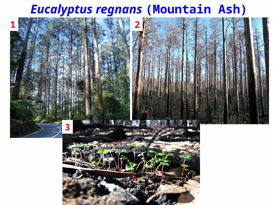
Eucalyptus regnans (Mountain Ash)1 2

3

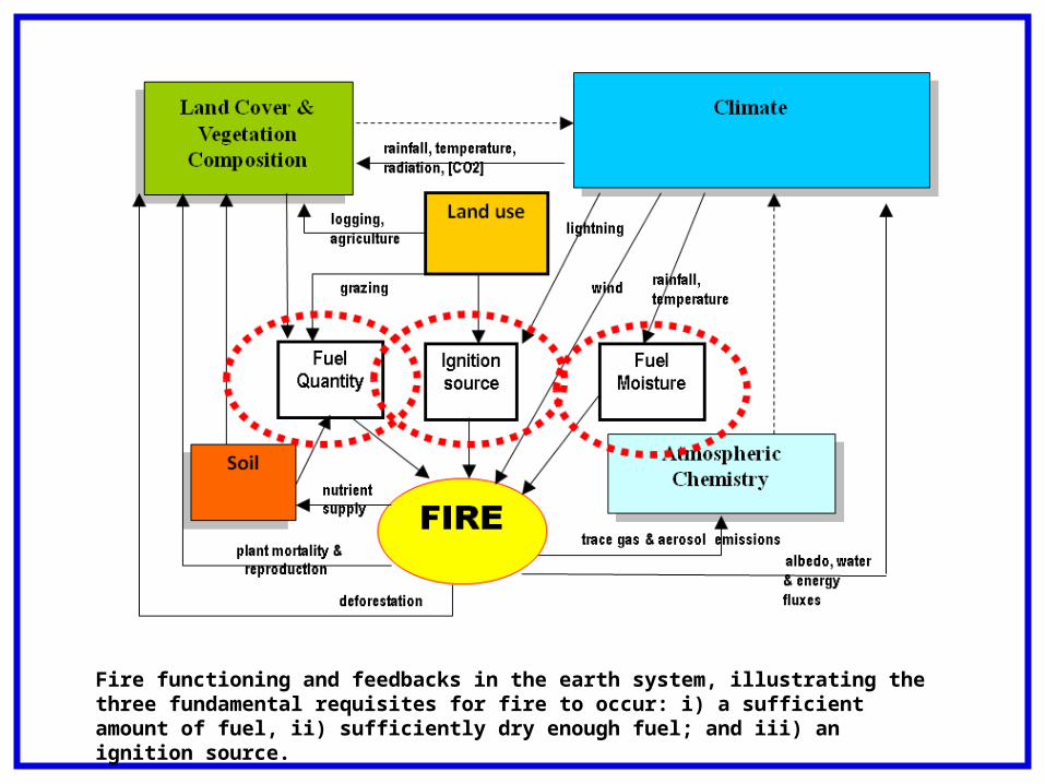
Fire functioning and feedbacks in the earth system, illustrating the three fundamental requisites for fire to occur: i) a sufficient amount of fuel, ii) sufficiently dry enough fuel; and iii) an ignition source.

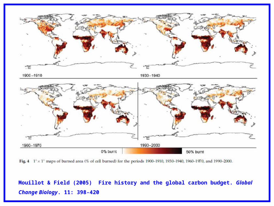
Mouillot & Field (2005) Fire history and the global carbon budget. Global Change Biology. 11: 398-420

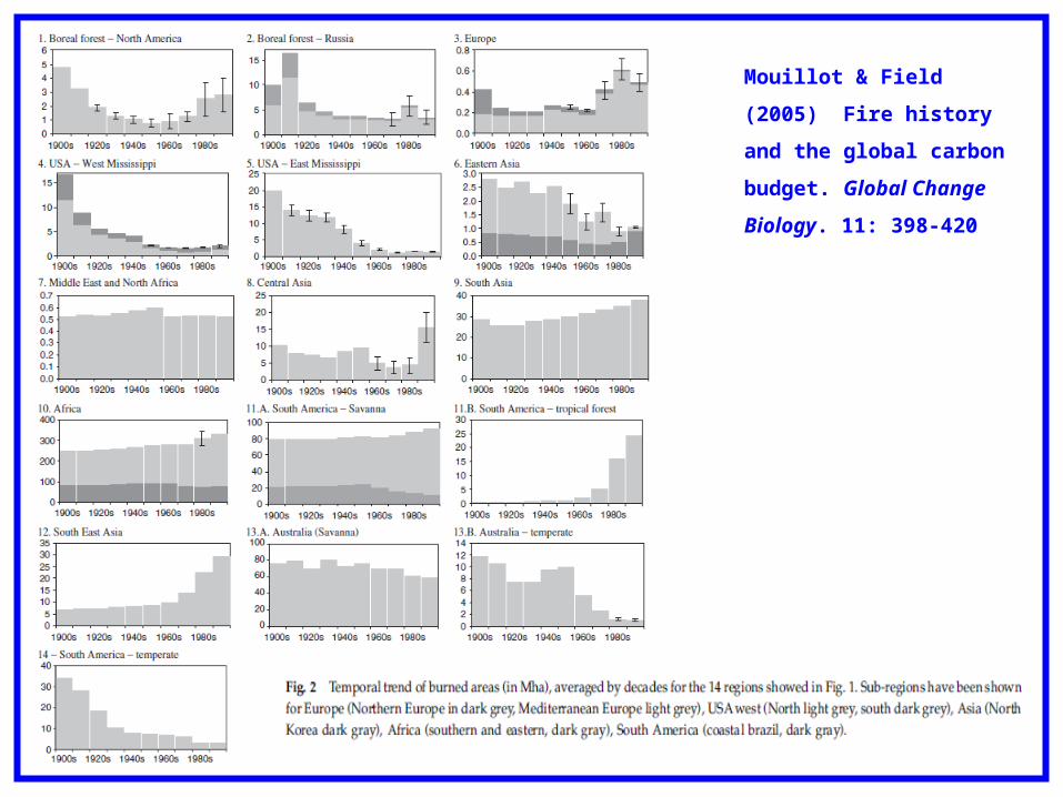
Mouillot & Field (2005) Fire

history and the global carbon

budget. Global Change

Biology. 11: 398-420

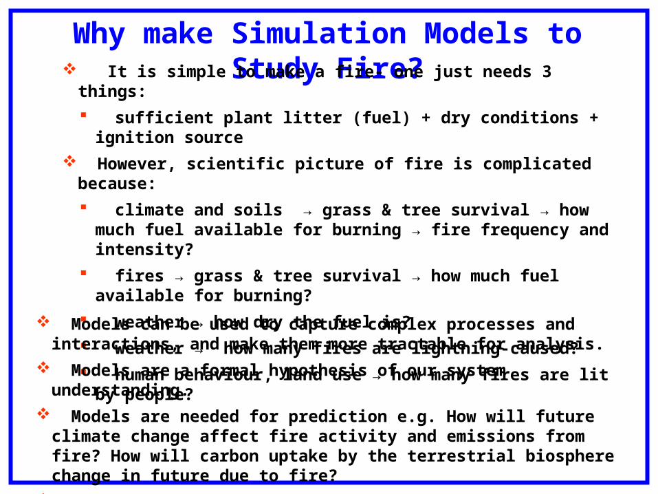
Why make Simulation Models to Study Fire? It is simple to make a fire- one just needs 3 things:

sufficient plant litter (fuel) + dry conditions + ignition source

However, scientific picture of fire is complicated because:

climate and soils → grass & tree survival → how much fuel available for burning → fire frequency and intensity?

fires → grass & tree survival → how much fuel available for burning?

weather → how dry the fuel is?

weather → how many fires are lightning-caused?

human behaviour, land use → how many fires are lit by people?

Models can be used to capture complex processes and interactions, and make them more tractable for analysis.

Models are a formal hypothesis of our system understanding.

Models are needed for prediction e.g. How will future climate change affect fire activity and emissions from fire? How will carbon uptake by the terrestrial biosphere change in future due to fire?

But model development and validation must precede interesting applications…

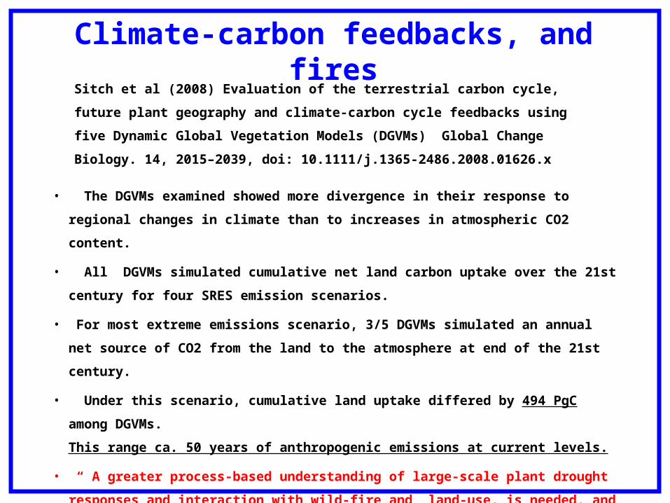
Climate-carbon feedbacks, and fires

Sitch et al (2008) Evaluation of the terrestrial carbon cycle, future plant geography and

climate-carbon cycle feedbacks using five Dynamic Global Vegetation Models (DGVMs)

Global Change Biology. 14, 2015–2039, doi: 10.1111/j.1365-2486.2008.01626.x

• The DGVMs examined showed more divergence in their response to regional changes in climate

than to increases in atmospheric CO2 content.

• All DGVMs simulated cumulative net land carbon uptake over the 21st century for four SRES

emission scenarios.

• For most extreme emissions scenario, 3/5 DGVMs simulated an annual net source of CO2 from

the land to the atmosphere at end of the 21st century.

• Under this scenario, cumulative land uptake differed by 494 PgC among DGVMs.

This range ca. 50 years of anthropogenic emissions at current levels.

• “ A greater process-based understanding of large-scale plant drought responses and interaction

with wild-fire and land-use, is needed, and this should filter into the next generation of DGVMs. “

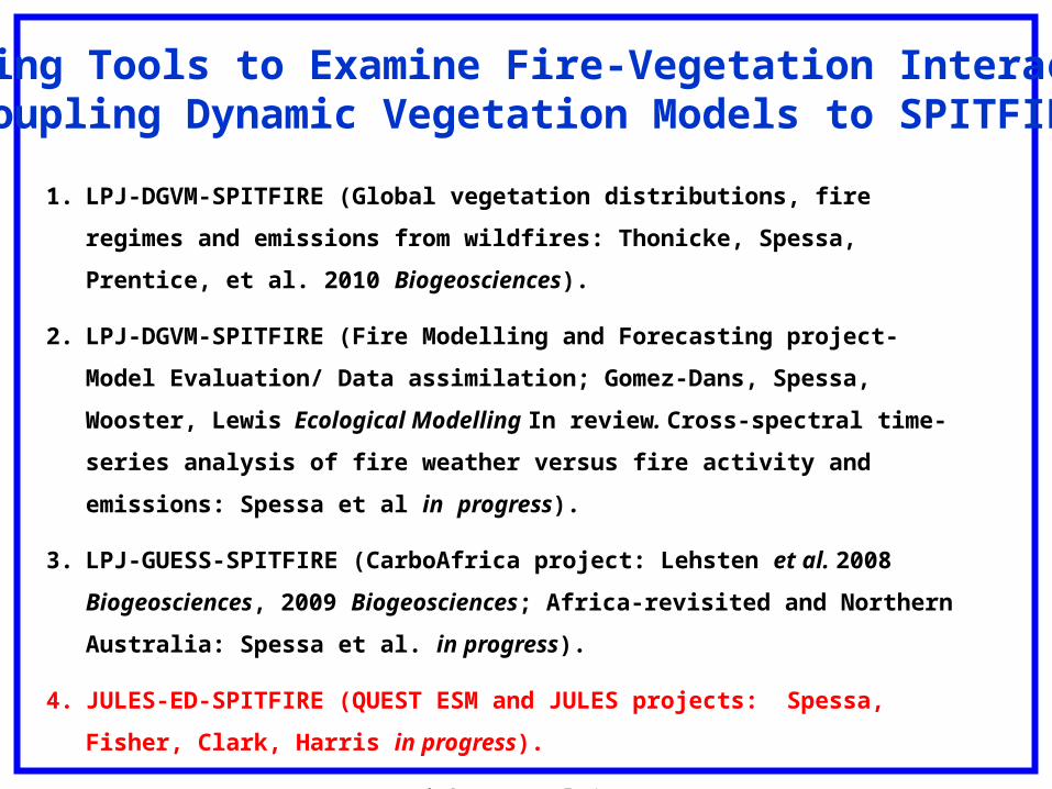
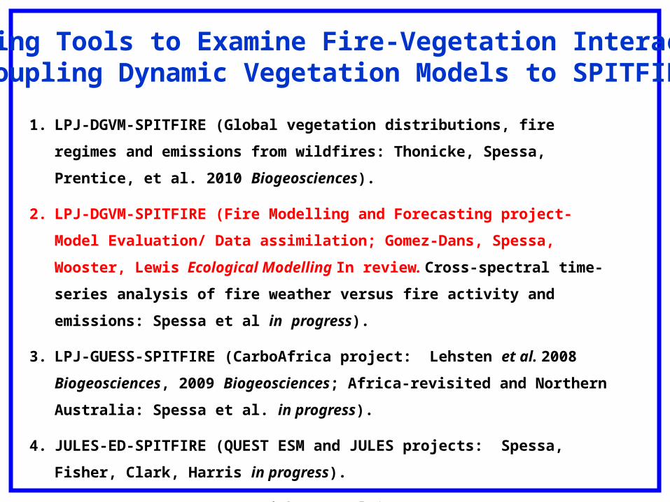
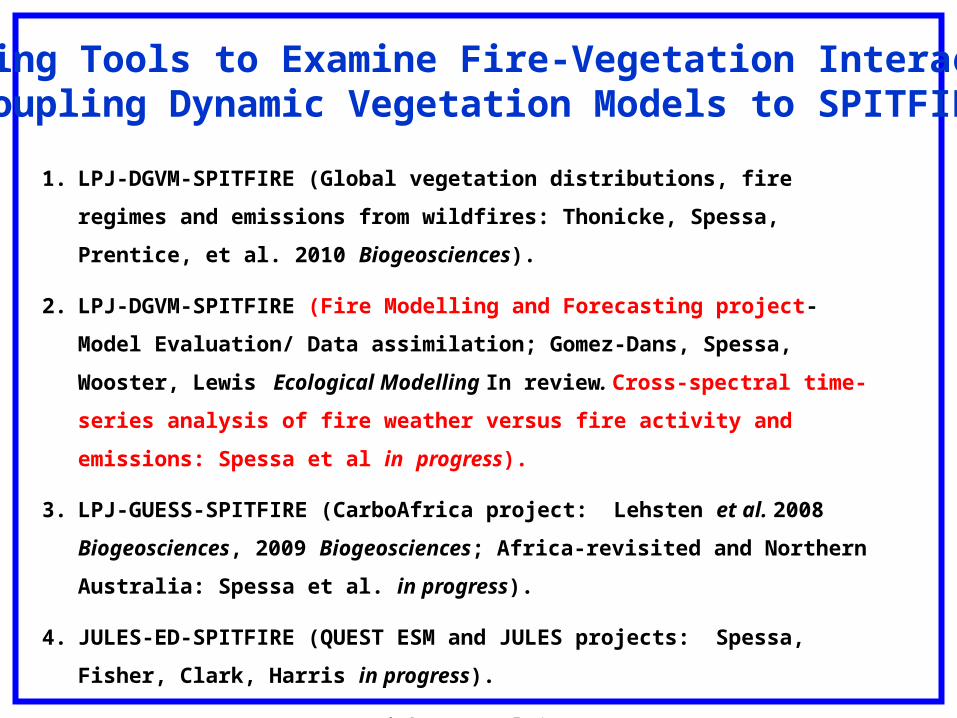
Building Tools to Examine Fire-Vegetation Interactions:Coupling Dynamic Vegetation Models to SPITFIRE

1. LPJ-DGVM-SPITFIRE (Global vegetation distributions, fire regimes and emissions from

wildfires: Thonicke, Spessa, Prentice, et al. 2010 Biogeosciences).

2. LPJ-DGVM-SPITFIRE (Fire Modelling and Forecasting project- Model Evaluation/ Data

assimilation; Gomez-Dans, Spessa, Wooster, Lewis Ecological Modelling In review.

Cross-spectral time-series analysis of fire weather versus fire activity and emissions:

Spessa et al in progress).

3. LPJ-GUESS-SPITFIRE (CarboAfrica project: Lehsten et al. 2008 Biogeosciences, 2009

Biogeosciences; Africa-revisited and Northern Australia: Spessa et al. in progress).

4. JULES-ED-SPITFIRE (QUEST ESM and JULES projects: Spessa, Fisher, Clark, Harris

in progress).

5. CLM-ED-SPITFIRE (NCAR: Fisher et al in progress.).

6. JSBACH-SPITFIRE (MPI-Met: Kloster et al in progress.).

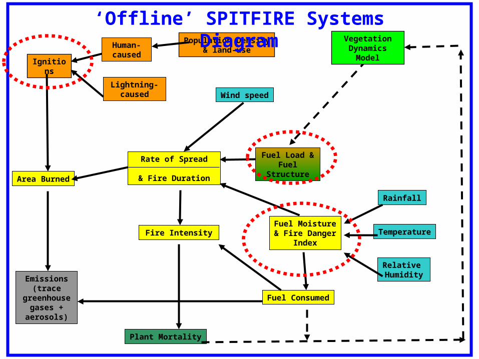
Ignitions

Fuel Consumed

Area Burned

Fuel Moisture& Fire Danger

Index

Rate of Spread

& Fire Duration

Fire Intensity

Emissions (trace

greenhouse gases +

aerosols)

Human-caused

Lightning-caused

Plant Mortality

Fuel Load &Fuel Structure

Wind speed

Temperature

Relative Humidity

Rainfall

Vegetation Dynamics Model

Population Density& land-use

‘Offline’ SPITFIRE Systems Diagram

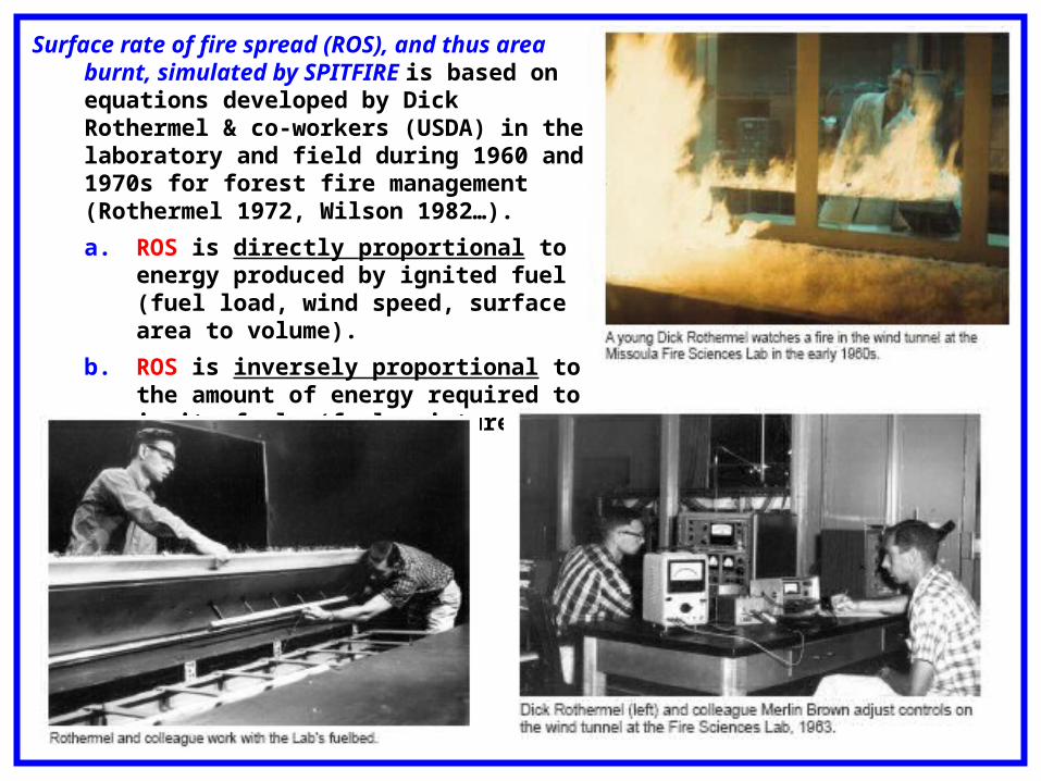
Surface rate of fire spread (ROS), and thus area burnt, simulated by SPITFIRE is based on equations developed by Dick Rothermel & co-workers (USDA) in the laboratory and field during 1960 and 1970s for forest fire management (Rothermel 1972, Wilson 1982…).

a. ROS is directly proportional to energy produced by ignited fuel (fuel load, wind speed, surface area to volume).

b. ROS is inversely proportional to the amount of energy required to ignite fuels (fuel moisture & fuel bulk density).

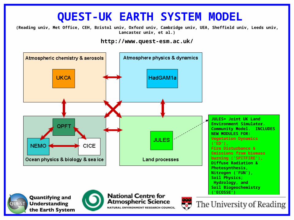
QUEST-UK EARTH SYSTEM MODEL(Reading univ, Met Office, CEH, Bristol univ, Oxford univ, Cambridge univ, UEA, Sheffield univ, Leeds univ, Lancaster

univ, et al.)

http://www.quest-esm.ac.uk/

JULES= Joint UK Land Environment Simulator. Community Model. INCLUDES NEW MODULES FOR:Vegetation Dynamics (‘ED’),Fire Disturbance & Emissions from biomass burning (‘SPITFIRE’),Diffuse Radiation & Photosynthesis, Nitrogen (‘FUN’),Soil Physics; Hydrology, andSoil Biogeochemistry (‘ECOSSE’)

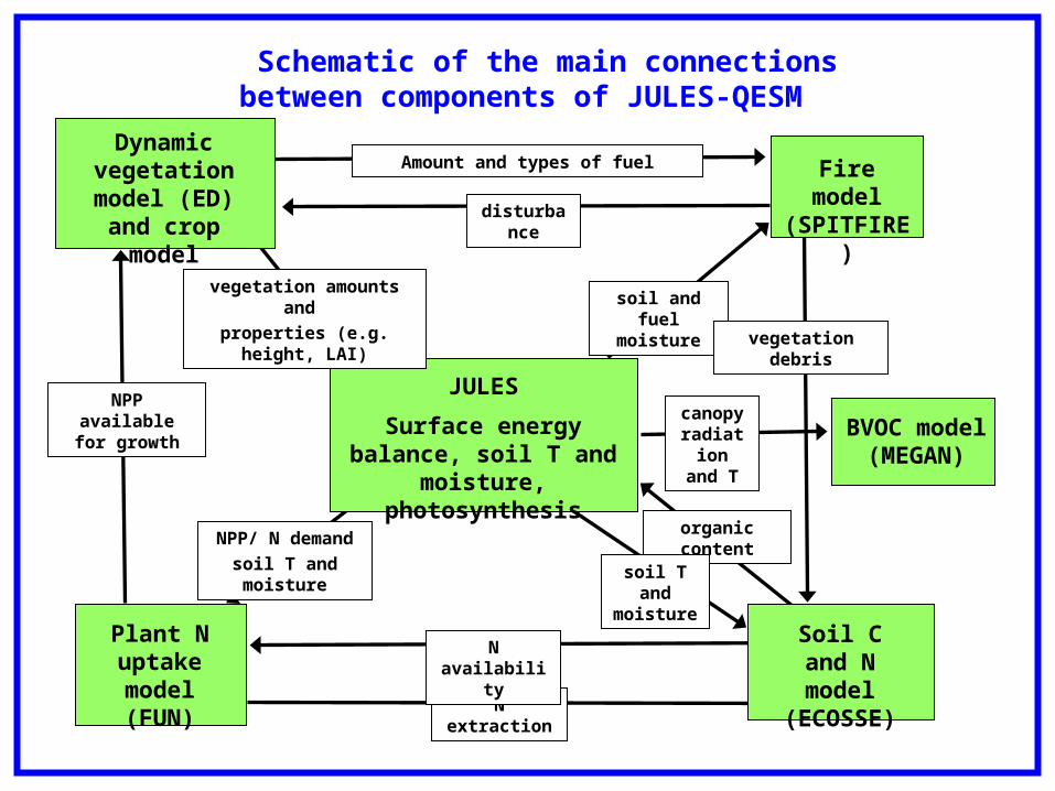
Schematic of the main connections between components of JULES-QESM

JULES

Surface energy balance, soil T and moisture, photosynthesis

Dynamic vegetation

model (ED) and crop model

Soil C and N model

(ECOSSE)

Plant N uptake model (FUN)

Fire model (SPITFIRE)

NPP/ N demand

soil T and moisture

disturbance

Amount and types of fuel

NPP available for growth

organic content

BVOC model (MEGAN)

soil and fuel moisture

N extraction

N availability

soil T and moisture

vegetation amounts and

properties (e.g. height, LAI)

canopy radiation

and T

vegetation debris

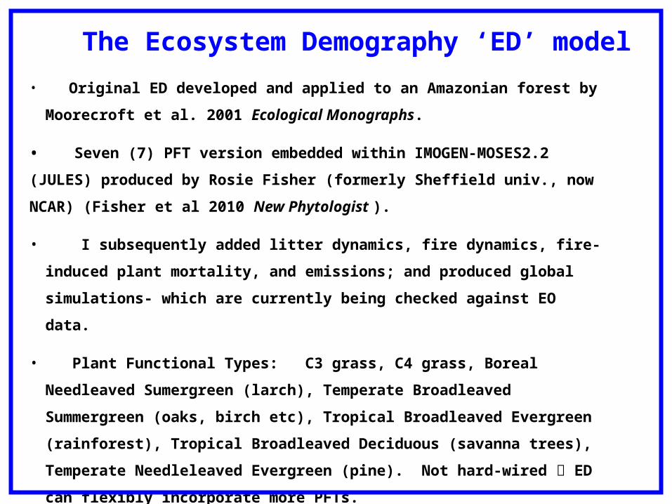
• Original ED developed and applied to an Amazonian forest by Moorecroft et al. 2001

Ecological Monographs.

•    Seven (7) PFT version embedded within IMOGEN-MOSES2.2 (JULES) produced by

Rosie Fisher (formerly Sheffield univ., now NCAR) (Fisher et al 2010 New Phytologist ).

• I subsequently added litter dynamics, fire dynamics, fire-induced plant mortality,

and emissions; and produced global simulations- which are currently being checked

against EO data.

• Plant Functional Types: C3 grass, C4 grass, Boreal Needleaved Sumergreen (larch),

Temperate Broadleaved Summergreen (oaks, birch etc), Tropical Broadleaved

Evergreen (rainforest), Tropical Broadleaved Deciduous (savanna trees), Temperate

Needleleaved Evergreen (pine). Not hard-wired ED can flexibly incorporate more

PFTs.

• ED is based on ‘gap’ model principles and the concepts of patches and cohorts. Quite

different from traditional DGVMs (eg LPJ, TRIFFID, BETHy etc).

The Ecosystem Demography ‘ED’ model

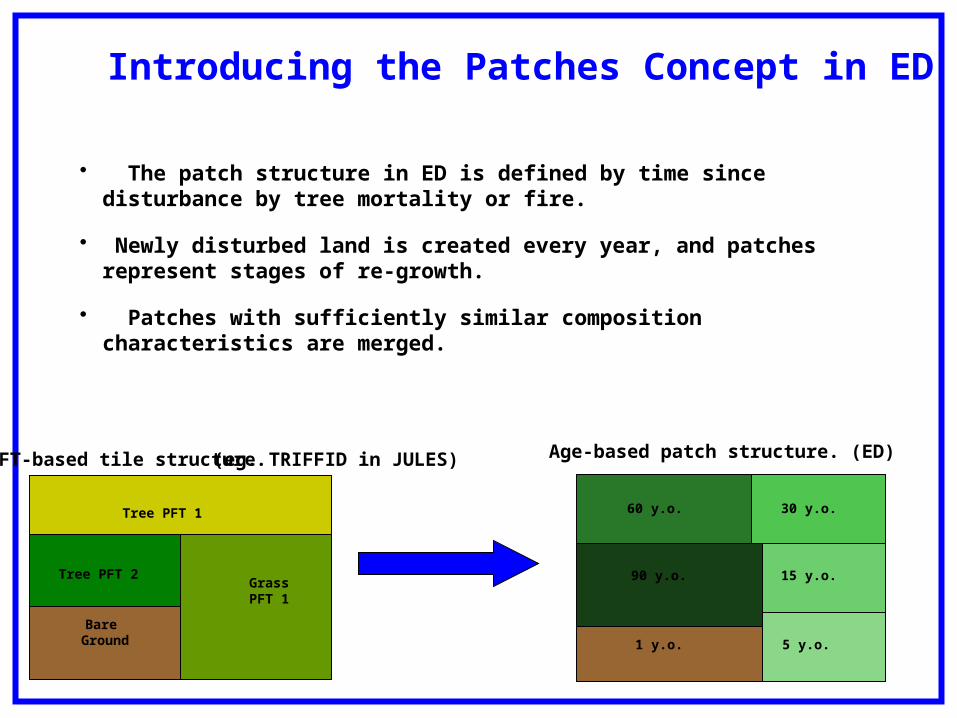
Introducing the Patches Concept in ED

Bare Ground

GrassPFT 1

Tree PFT 1

Tree PFT 2

1 y.o. 5 y.o.

15 y.o.

30 y.o.60 y.o.

90 y.o.

(eg. TRIFFID in JULES) Age-based patch structure. (ED)PFT-based tile structure.

• The patch structure in ED is defined by time since disturbance by tree mortality or fire.

• Newly disturbed land is created every year, and patches represent stages of re-growth.

• Patches with sufficiently similar composition characteristics are merged.

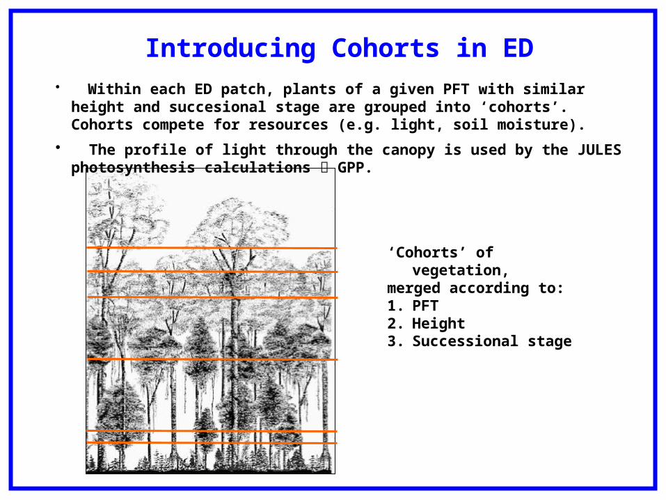
Introducing Cohorts in ED

‘Cohorts’ of vegetation,merged according to:1. PFT2. Height3. Successional stage

• Within each ED patch, plants of a given PFT with similar height and succesional stage are grouped into ‘cohorts’. Cohorts compete for resources (e.g. light, soil moisture).

• The profile of light through the canopy is used by the JULES photosynthesis calculations GPP.

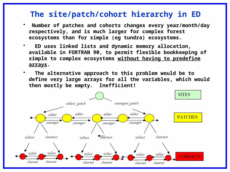
The site/patch/cohort hierarchy in ED

• Number of patches and cohorts changes every year/month/day respectively, and is much larger for complex forest ecosystems than for simple (eg tundra) ecosystems.

• ED uses linked lists and dynamic memory allocation, available in FORTRAN 90, to permit flexible bookkeeping of simple to complex ecosystems without having to predefine arrays.

• The alternative approach to this problem would be to define very large arrays for all the variables, which would then mostly be empty. Inefficient!

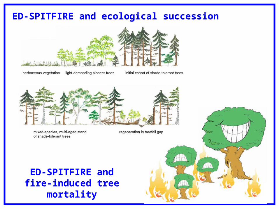
ED-SPITFIRE and ecological succession

ED-SPITFIRE andfire-induced tree

mortality

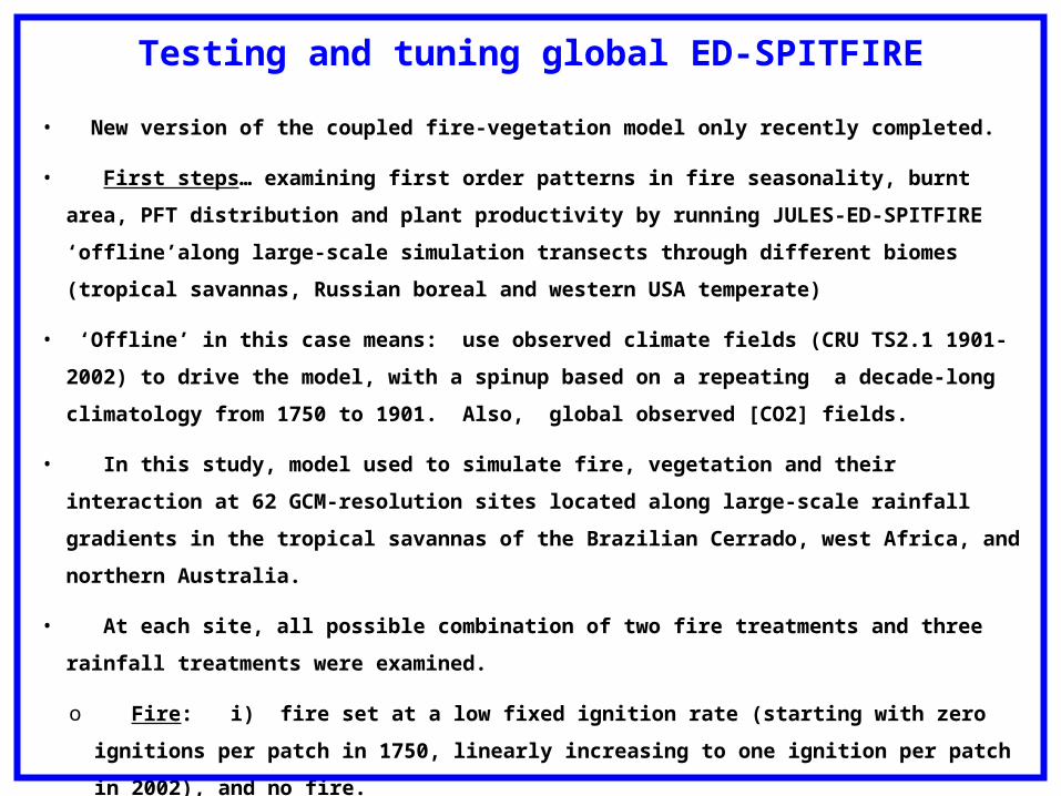
Testing and tuning global ED-SPITFIRE

• New version of the coupled fire-vegetation model only recently completed.

• First steps… examining first order patterns in fire seasonality, burnt area, PFT distribution and plant

productivity by running JULES-ED-SPITFIRE ‘offline’along large-scale simulation transects through

different biomes (tropical savannas, Russian boreal and western USA temperate)

• ‘Offline’ in this case means: use observed climate fields (CRU TS2.1 1901-2002) to drive the model, with a

spinup based on a repeating a decade-long climatology from 1750 to 1901. Also, global observed [CO2]

fields.

• In this study, model used to simulate fire, vegetation and their interaction at 62 GCM-resolution sites

located along large-scale rainfall gradients in the tropical savannas of the Brazilian Cerrado, west Africa,

and northern Australia.

• At each site, all possible combination of two fire treatments and three rainfall treatments were examined.

o Fire: i) fire set at a low fixed ignition rate (starting with zero ignitions per patch in 1750, linearly

increasing to one ignition per patch in 2002), and no fire.

o Rainfall: i) -20% of daily rainfall, ii) no change to daily rainfall, and iii) +20% of daily rainfall.

• No influence of humans/land use or lightning in these experiments.

• Natural vegetation only ie. no agricultural land.

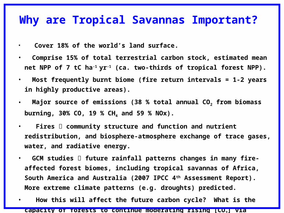
• Cover 18% of the world’s land surface.

• Comprise 15% of total terrestrial carbon stock, estimated mean net NPP of 7 tC ha-1 yr-1

(ca. two-thirds of tropical forest NPP).

• Most frequently burnt biome (fire return intervals = 1-2 years in highly productive areas).

• Major source of emissions (38 % total annual CO2 from biomass burning, 30% CO, 19 %

CH4 and 59 % NOx).

• Fires community structure and function and nutrient redistribution, and biosphere-

atmosphere exchange of trace gases, water, and radiative energy.

• GCM studies future rainfall patterns changes in many fire-affected forest biomes,

including tropical savannas of Africa, South America and Australia (2007 IPCC 4th

Assessment Report). More extreme climate patterns (e.g. droughts) predicted.

• How this will affect the future carbon cycle? What is the capacity of forests to continue

moderating rising [CO2] via carbon sequestration?

• How well can we simulate contemporary vegetation dynamics, fire dynamics, and fire-

vegetation interactions?

Why are Tropical Savannas Important?

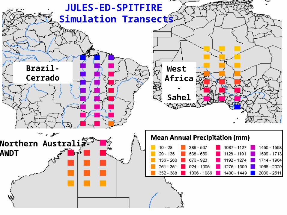
JULES-ED-SPITFIRE Simulation Transects

Brazil- Cerrado West Africa- Sahel

Northern Australia-AWDT

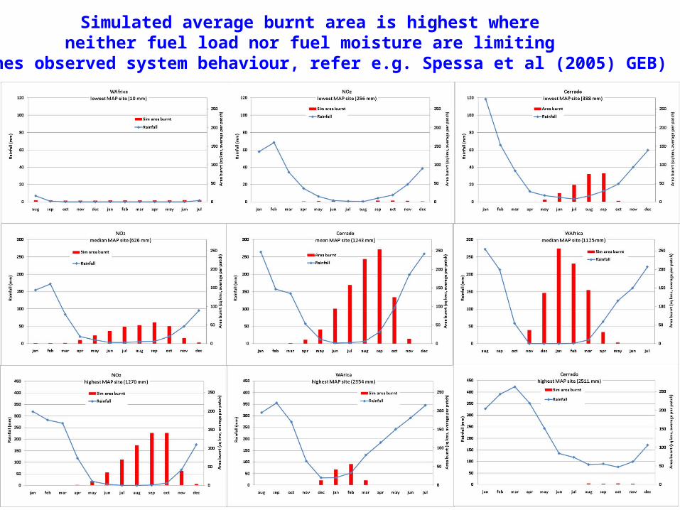
Simulated average burnt area is highest where neither fuel load nor fuel moisture are limiting

(matches observed system behaviour, refer e.g. Spessa et al (2005) GEB)

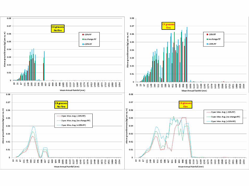
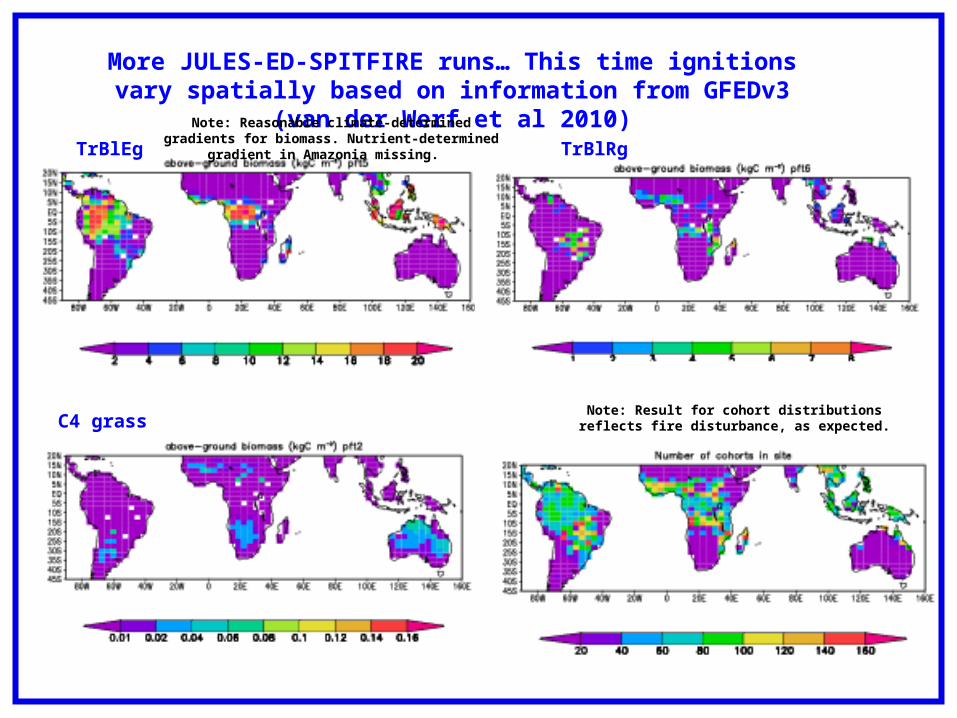
More JULES-ED-SPITFIRE runs… This time ignitions vary spatially based on information from GFEDv3 (van der Werf et al 2010)

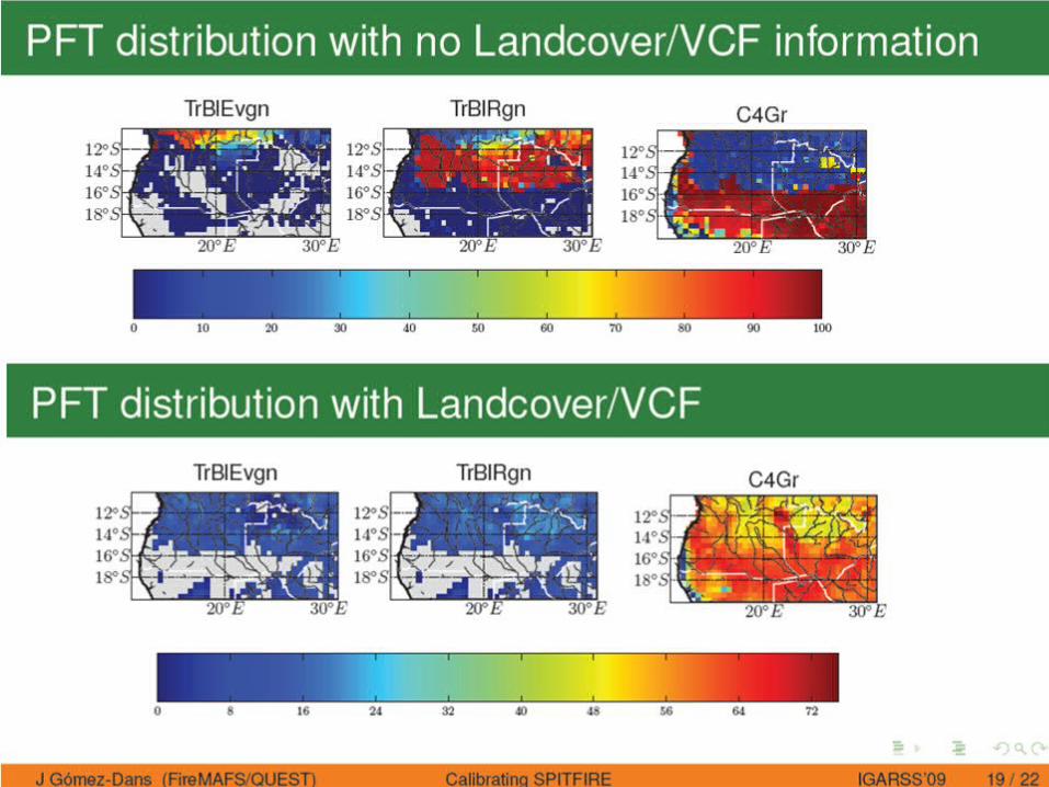
TrBlEg TrBlRg

C4 grass

Note: Reasonable climate-determined gradients for biomass. Nutrient-determined gradient in Amazonia missing.

Note: Result for cohort distributions reflects fire disturbance, as expected.

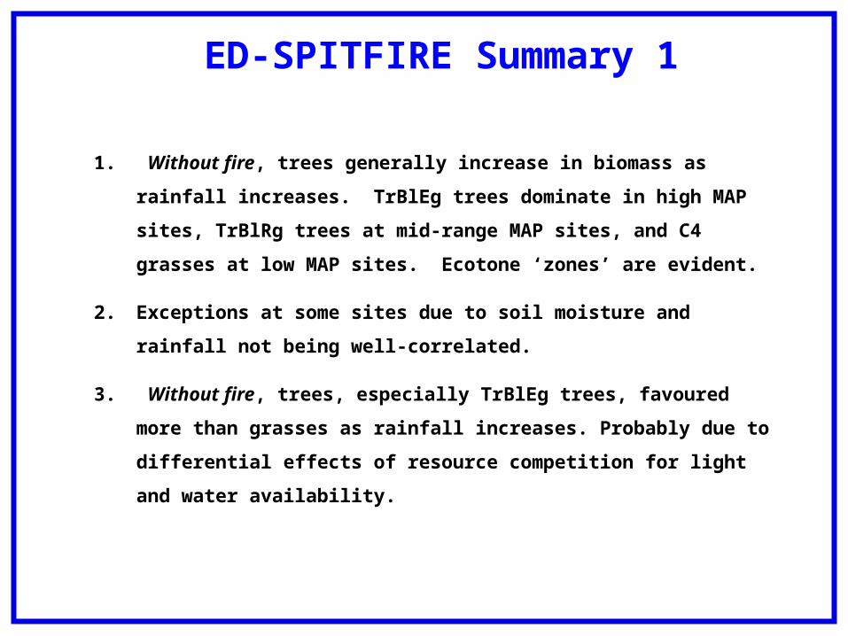
ED-SPITFIRE Summary 1

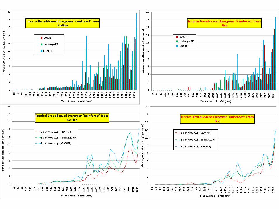
1. Without fire, trees generally increase in biomass as rainfall increases. TrBlEg

trees dominate in high MAP sites, TrBlRg trees at mid-range MAP sites, and C4

grasses at low MAP sites. Ecotone ‘zones’ are evident.

2. Exceptions at some sites due to soil moisture and rainfall not being well-

correlated.

3. Without fire, trees, especially TrBlEg trees, favoured more than grasses as

rainfall increases. Probably due to differential effects of resource competition

for light and water availability.

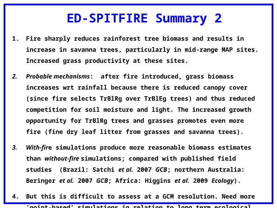
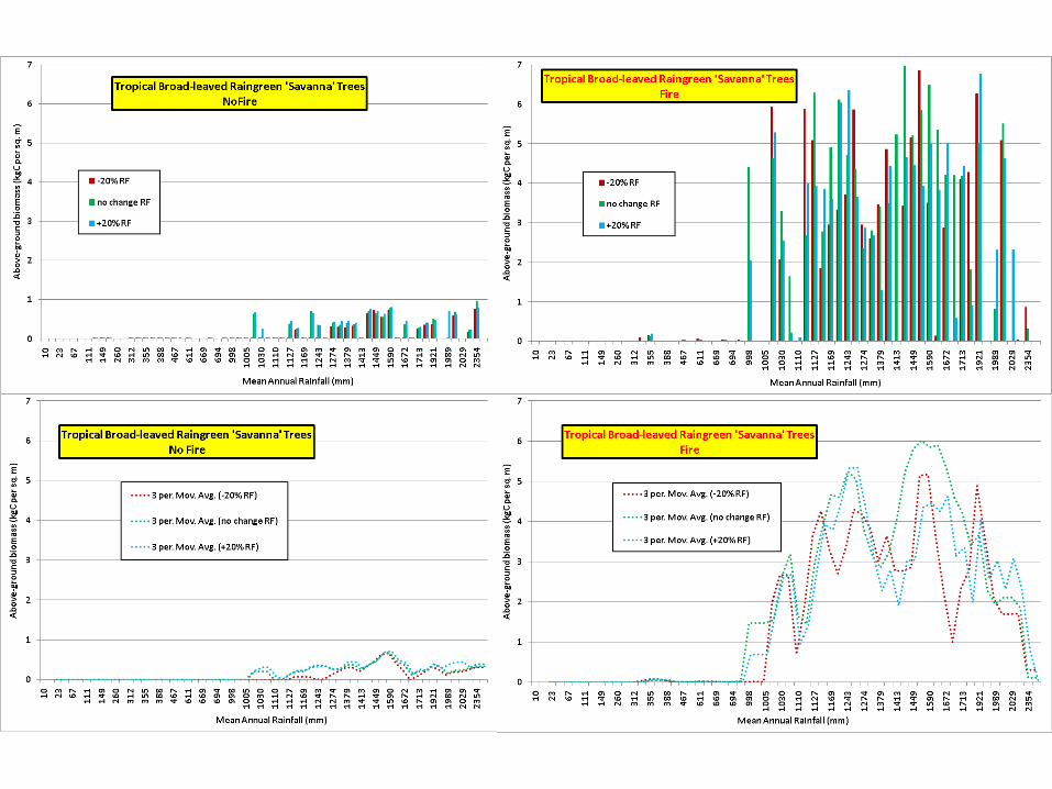
ED-SPITFIRE Summary 21. Fire sharply reduces rainforest tree biomass and results in increase in savanna trees,

particularly in mid-range MAP sites. Increased grass productivity at these sites.

2. Probable mechanisms: after fire introduced, grass biomass increases wrt rainfall because

there is reduced canopy cover (since fire selects TrBlRg over TrBlEg trees) and thus

reduced competition for soil moisture and light. The increased growth opportunity for

TrBlRg trees and grasses promotes even more fire (fine dry leaf litter from grasses and

savanna trees).

3. With-fire simulations produce more reasonable biomass estimates than without-fire

simulations; compared with published field studies (Brazil: Satchi et al. 2007 GCB;

northern Australia: Beringer et al. 2007 GCB; Africa: Higgins et al. 2009 Ecology).

4. But this is difficult to assess at a GCM resolution. Need more ‘point-based’ simulations in

relation to long term ecological experiments that control fire treatments (unfortunately

few available).

Building Tools to Examine Fire-Vegetation Interactions:Coupling Dynamic Vegetation Models to SPITFIRE

1. LPJ-DGVM-SPITFIRE (Global vegetation distributions, fire regimes and emissions from

wildfires: Thonicke, Spessa, Prentice, et al. 2010 Biogeosciences).

2. LPJ-DGVM-SPITFIRE (Fire Modelling and Forecasting project- Model Evaluation/ Data

assimilation; Gomez-Dans, Spessa, Wooster, Lewis Ecological Modelling In review.

Cross-spectral time-series analysis of fire weather versus fire activity and emissions:

Spessa et al in progress).

3. LPJ-GUESS-SPITFIRE (CarboAfrica project: Lehsten et al. 2008 Biogeosciences, 2009

Biogeosciences; Africa-revisited and Northern Australia: Spessa et al. in progress).

4. JULES-ED-SPITFIRE (QUEST ESM and JULES projects: Spessa, Fisher, Clark, Harris

in progress).

5. CLM-ED-SPITFIRE (NCAR: Fisher et al in progress.).

6. JSBACH-SPITFIRE (MPI-Met: Kloster et al in progress.).

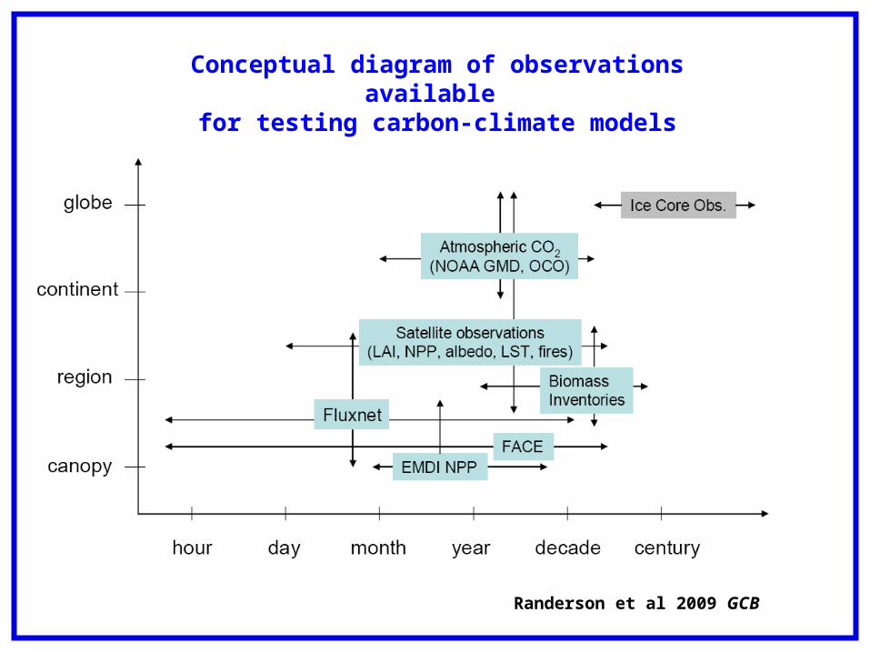
Conceptual diagram of observations available for testing carbon-climate models

Randerson et al 2009 GCB

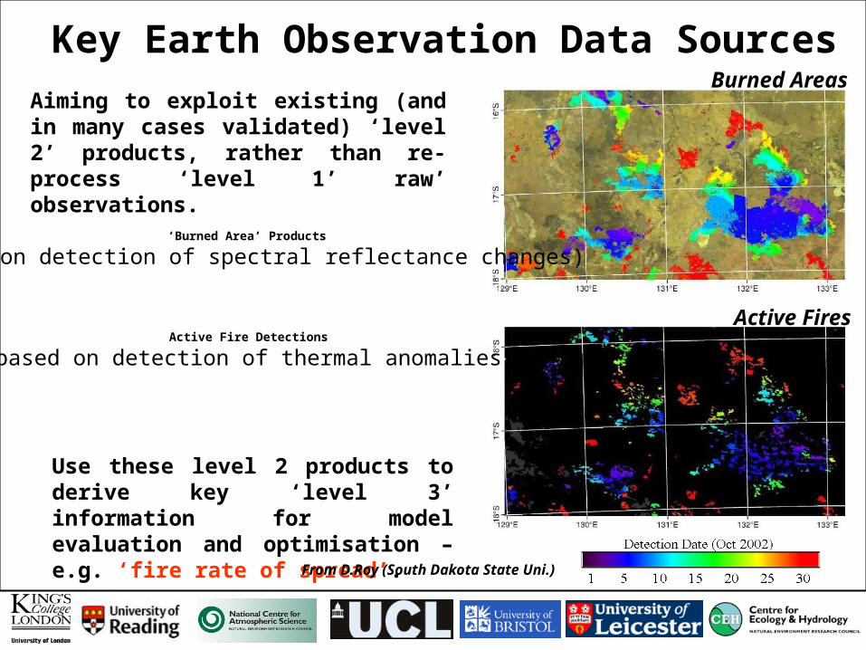
Active Fire Detections

(based on detection of thermal anomalies)

‘Burned Area’ Products

(based on detection of spectral reflectance changes)

Key Earth Observation Data Sources

Aiming to exploit existing (and in many cases validated) ‘level 2’ products, rather than re-process ‘level 1’ raw’ observations.

Burned Areas

Active Fires

Use these level 2 products to derive key ‘level 3’ information for model evaluation and optimisation – e.g. ‘fire rate of spread’.

From D.Roy (South Dakota State Uni.)

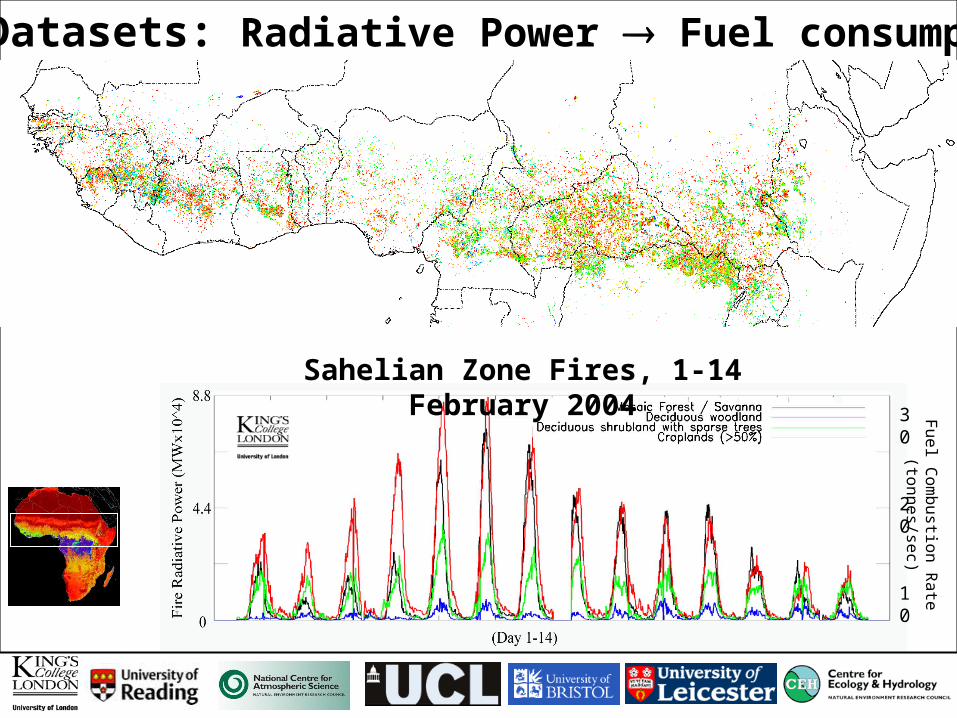
Sahelian Zone Fires, 1-14 February 2004

Fuel C

ombustion R

ate (tonnes/sec)

30

20

10

0

Key Datasets: Radiative Power Fuel consumption

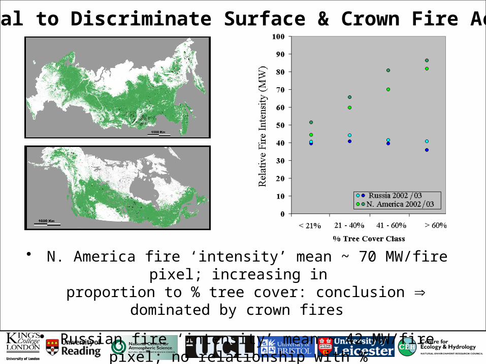
• N. America fire ‘intensity’ mean ~ 70 MW/fire pixel; increasing in proportion to % tree cover: conclusion dominated by crown fires

• Russian fire ‘intensity’ mean ~ 42 MW/fire pixel; no relationship with %

tree cover: conclusion dominated by surface fires

Potential to Discriminate Surface & Crown Fire Activity

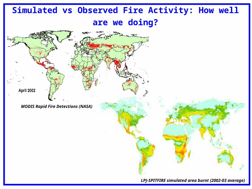
Simulated vs Observed Fire Activity: How well are we doing?

MODIS Rapid Fire Detections (NASA)

LPJ-SPITFIRE simulated area burnt (2002-03 average)

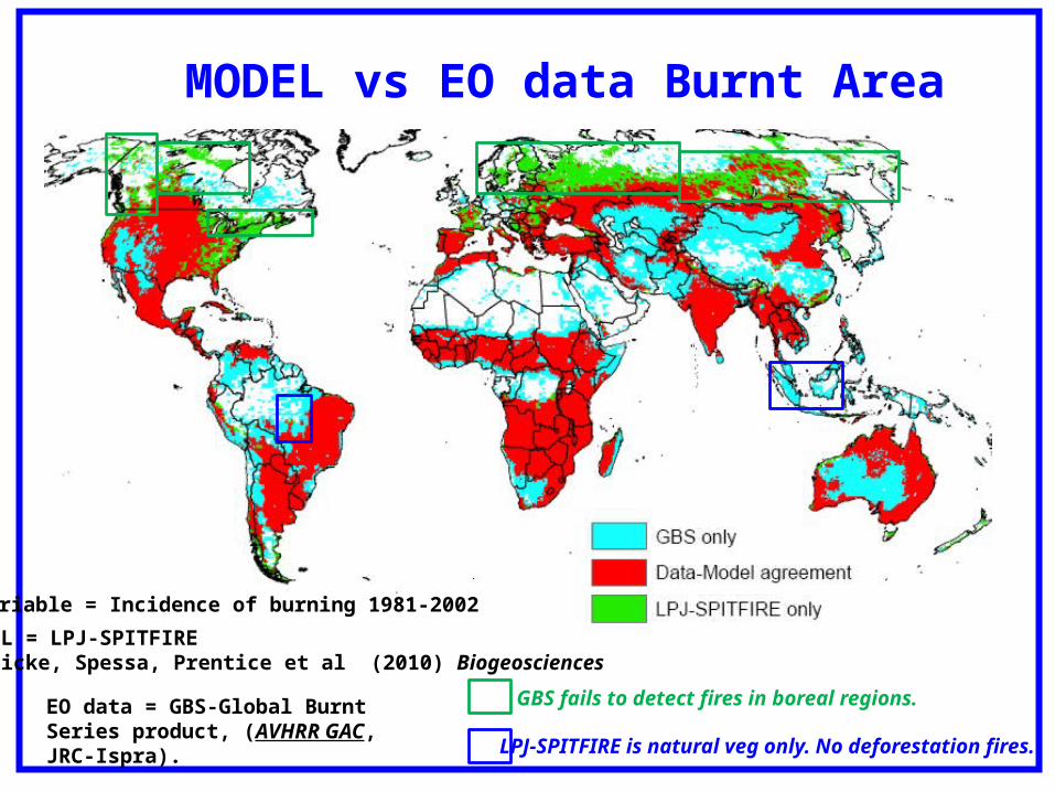
MODEL vs EO data Burnt Area

EO data = GBS-Global Burnt Series product, (AVHRR GAC, JRC-Ispra).

MODEL = LPJ-SPITFIREThonicke, Spessa, Prentice et al (2010) Biogeosciences

Variable = Incidence of burning 1981-2002

GBS fails to detect fires in boreal regions.

LPJ-SPITFIRE is natural veg only. No deforestation fires.

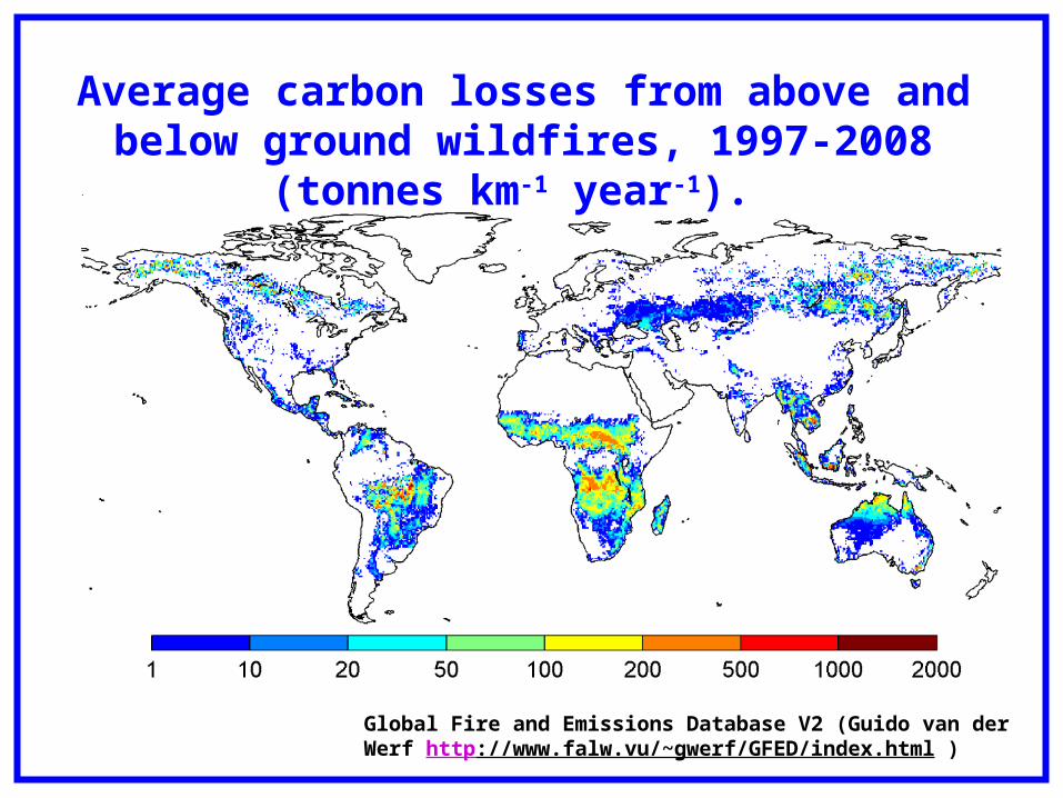
Average carbon losses from above and below ground wildfires, 1997-2008 (tonnes km-1 year-1).

Global Fire and Emissions Database V2 (Guido van der Werf http://www.falw.vu/~gwerf/GFED/index.html )

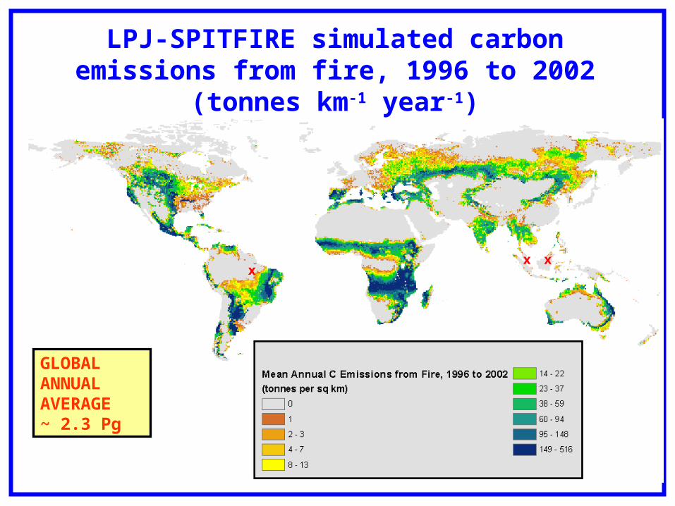
LPJ-SPITFIRE simulated carbon emissions from fire, 1996 to 2002 (tonnes km-1 year-1)

GLOBAL ANNUAL AVERAGE~ 2.3 Pg

xxx

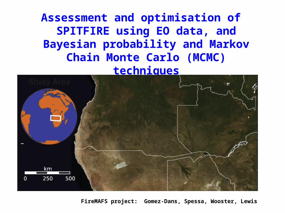
Assessment and optimisation of SPITFIRE using EO data, and Bayesian probability and Markov

Chain Monte Carlo (MCMC) techniques

FireMAFS project: Gomez-Dans, Spessa, Wooster, Lewis

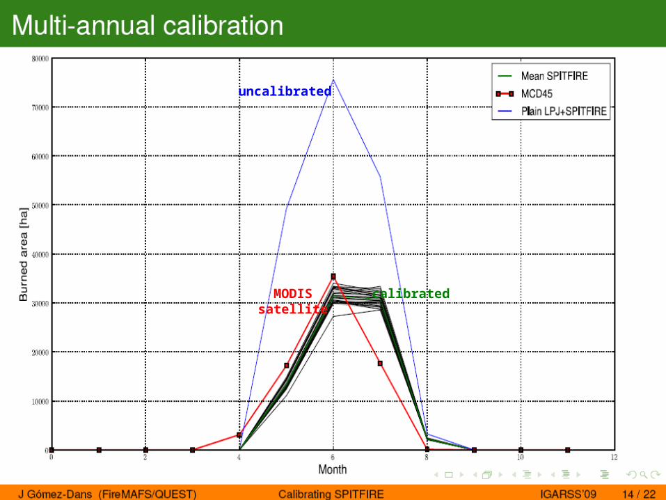
uncalibrated

calibratedMODISsatellite

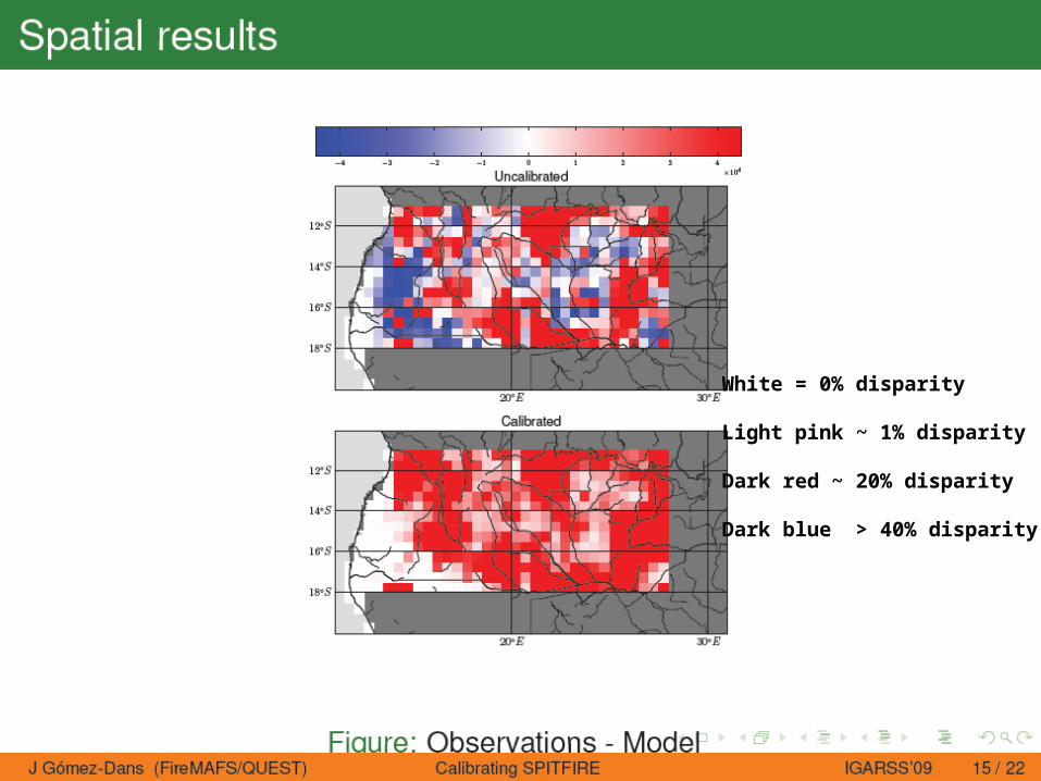
White = 0% disparity

Light pink ~ 1% disparity

Dark red ~ 20% disparity

Dark blue > 40% disparity.

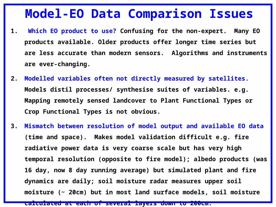
Model-EO Data Comparison Issues1. Which EO product to use? Confusing for the non-expert. Many EO products available.

Older products offer longer time series but are less accurate than modern sensors.

Algorithms and instruments are ever-changing.

2. Modelled variables often not directly measured by satellites. Models distil processes/

synthesise suites of variables. e.g. Mapping remotely sensed landcover to Plant Functional

Types or Crop Functional Types is not obvious.

3. Mismatch between resolution of model output and available EO data (time and space).

Makes model validation difficult e.g. fire radiative power data is very coarse scale but has

very high temporal resolution (opposite to fire model); albedo products (was 16 day, now 8

day running average) but simulated plant and fire dynamics are daily; soil moisture radar

measures upper soil moisture (~ 20cm) but in most land surface models, soil moisture

calculated at each of several layers down to 200cm.

4. EO data is NOT truth. User beware.

5. Closer dialogue between EO experts and modellers needed Precedence? Examples: C-

LAMP, ESA ‘Essential Climate Variables’ projects…

Building Tools to Examine Fire-Vegetation Interactions:Coupling Dynamic Vegetation Models to SPITFIRE

1. LPJ-DGVM-SPITFIRE (Global vegetation distributions, fire regimes and emissions from

wildfires: Thonicke, Spessa, Prentice, et al. 2010 Biogeosciences).

2. LPJ-DGVM-SPITFIRE (Fire Modelling and Forecasting project- Model Evaluation/ Data

assimilation; Gomez-Dans, Spessa, Wooster, Lewis Ecological Modelling In review.

Cross-spectral time-series analysis of fire weather versus fire activity and emissions:

Spessa et al in progress).

3. LPJ-GUESS-SPITFIRE (CarboAfrica project: Lehsten et al. 2008 Biogeosciences, 2009

Biogeosciences; Africa-revisited and Northern Australia: Spessa et al. in progress).

4. JULES-ED-SPITFIRE (QUEST ESM and JULES projects: Spessa, Fisher, Clark, Harris

in progress).

5. CLM-ED-SPITFIRE (NCAR: Fisher et al in progress.).

6. JSBACH-SPITFIRE (MPI-Met: Kloster et al in progress.).

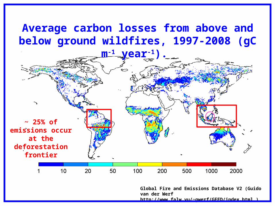
Average carbon losses from above and below ground wildfires, 1997-2008 (gC m-1 year-1).

Global Fire and Emissions Database V2 (Guido van der Werf http://www.falw.vu/~gwerf/GFED/index.html )

~ 25% of emissions occur at the

deforestation frontier

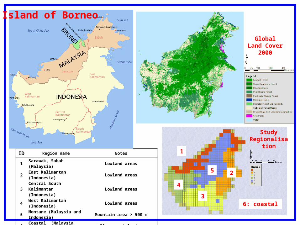
ID Region name Notes

1 Sarawak, Sabah (Malaysia) Lowland areas

2 East Kalimantan (Indonesia) Lowland areas

3 Central South Kalimantan (Indonesia) Lowland areas

4 West Kalimantan (Indonesia) Lowland areas

5 Montane (Malaysia and Indonesia) Mountain area > 500 m

6 Coastal (Malaysia and Indonesia) < 30 percent landmass

1

6: coastal

4

5 2

3

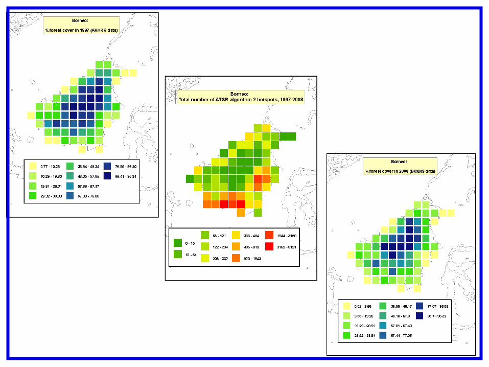
Island of Borneo

Global Land Cover 2000

Study Regionalisation

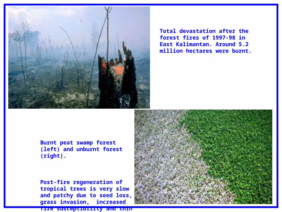
Burnt peat swamp forest (left) and unburnt forest (right).

Post-fire regeneration of tropical trees is very slow and patchy due to seed loss, grass invasion, increased fire susceptibility and thin bark of trees.

Total devastation after the forest fires of 1997-98 in East Kalimantan. Around 5.2 million hectares were burnt.

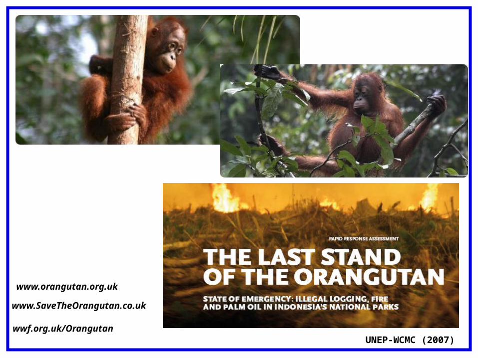
www.orangutan.org.uk

www.SaveTheOrangutan.co.uk

wwf.org.uk/OrangutanUNEP-WCMC (2007)

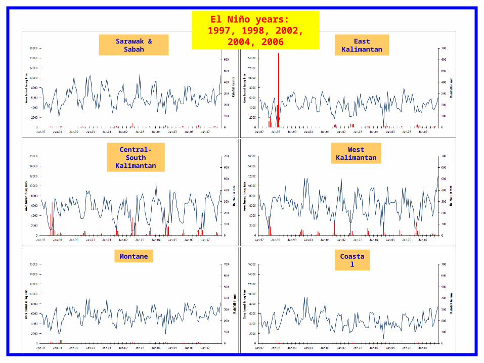
Sarawak & Sabah

Coastal

Central-South Kalimantan

Montane

West Kalimantan

EastKalimantan

El Niño years: 1997, 1998, 2002, 2004, 2006

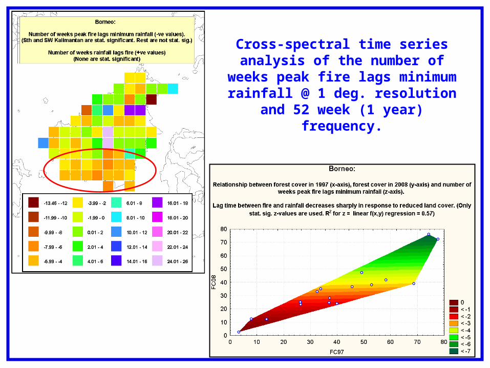
Cross-spectral time series analysis of the number of weeks peak fire lags

minimum rainfall @ 1 deg. resolution and 52 week (1 year) frequency.

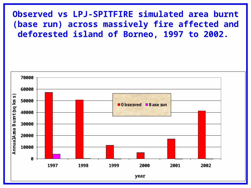
Observed vs LPJ-SPITFIRE simulated area burnt (base run) across massively fire affected and deforested island of Borneo,

1997 to 2002.

0

10000

20000

30000

40000

50000

60000

70000

1997 1998 1999 2000 2001 2002

An

nu

al A

rea

Bu

rnt

(sq

km

s)

year

Observed Base run

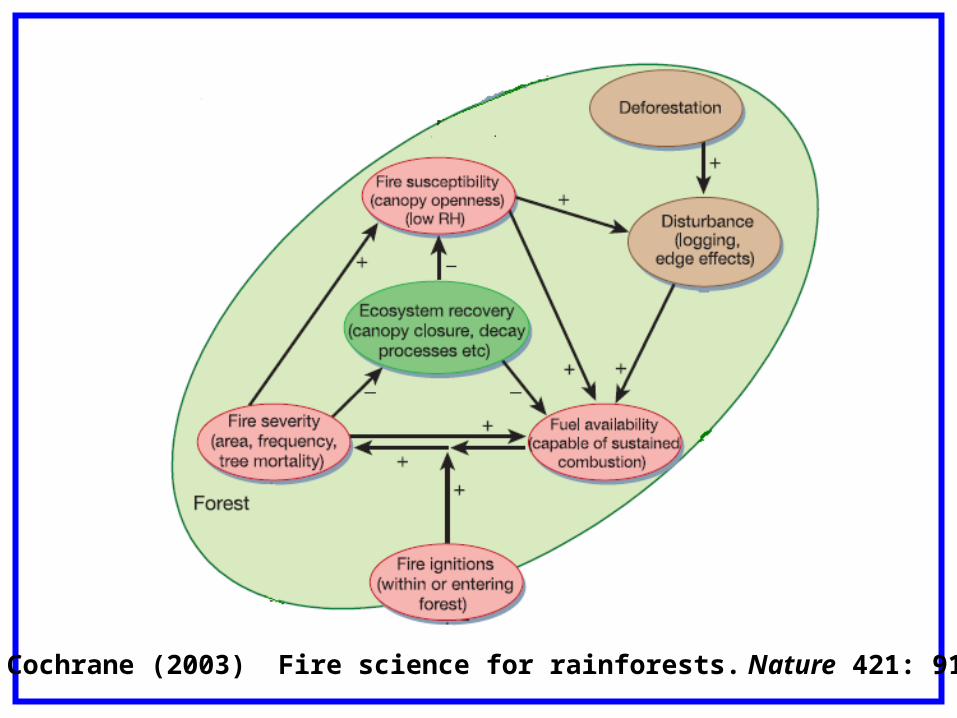
Cochrane (2003) Fire science for rainforests. Nature 421: 913-919

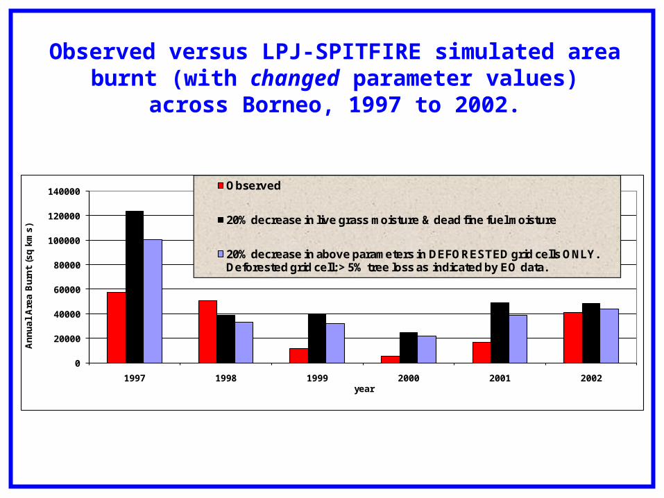
Observed versus LPJ-SPITFIRE simulated area burnt (with changed parameter values) across Borneo, 1997 to 2002.

0

20000

40000

60000

80000

100000

120000

140000

1997 1998 1999 2000 2001 2002

An

nu

al

Are

a B

urn

t (s

q k

ms

)

year

Observed

20% decrease in live grass moisture & dead fine fuel moisture

20% decrease in above parameters in DEFORESTED grid cells ONLY. Deforested grid cell: > 5% tree loss as indicated by EO data.

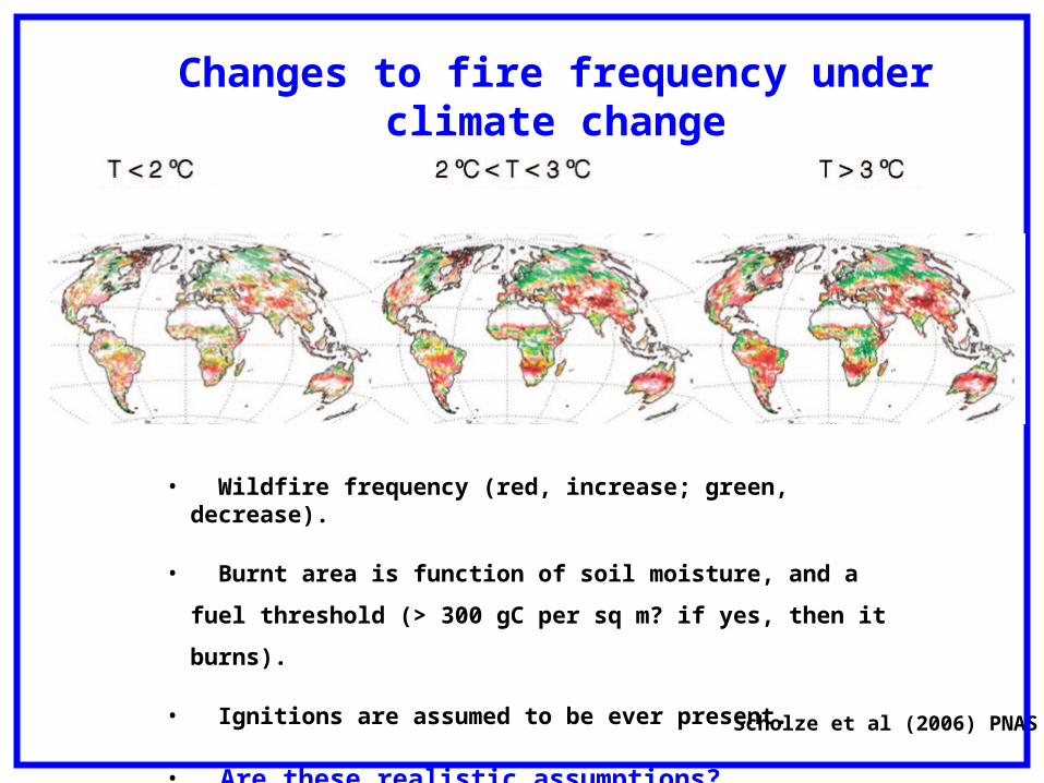
Scholze et al (2006) PNAS

Changes to fire frequency under climate change

• Wildfire frequency (red, increase; green, decrease).

• Burnt area is function of soil moisture, and a fuel threshold (> 300 gC

per sq m? if yes, then it burns).

• Ignitions are assumed to be ever present.

• Are these realistic assumptions?

George Pankiewicz © Crown copyright Met Office

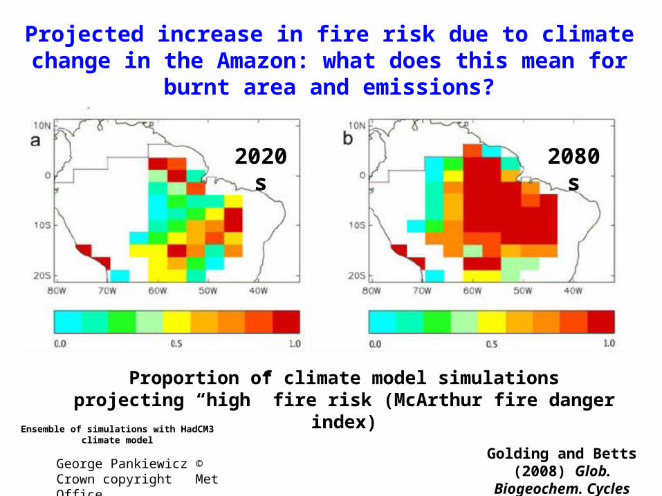
Projected increase in fire risk due to climate change in the Amazon: what does this mean for burnt area and emissions?

2020s 2080s

Proportion of climate model simulations projecting “high” fire risk (McArthur fire danger index)

Ensemble of simulations with HadCM3 climate model

Golding and Betts (2008) Glob. Biogeochem. Cycles

Fire functioning and feedbacks in the earth system, illustrating the three fundamental requisites for fire to occur: i) a sufficient amount of fuel, ii) sufficiently dry enough fuel; and iii) an ignition source.

Thank you for your attention!