Master of Science Thesis in Electrical EngineeringDepartment of Electrical Engineering, Linköping University, 2016

Global Illumination inReal-Time using VoxelCone Tracing on MobileDevices

Conrad Wahlén

Master of Science Thesis in Electrical Engineering

Global Illumination in Real-Time using Voxel Cone Tracing on Mobile Devices

Conrad Wahlén

LiTH-ISY-EX–16/5011–SE

Supervisor: Åsa DetterfeltCEO, Mindroad

Mikael Perssonisy, Linköpings universitet

Examiner: Ingemar Ragnemalmisy, Linköpings universitet

Division of Information CodingDepartment of Electrical Engineering

Linköping UniversitySE-581 83 Linköping, Sweden

Copyright © 2016 Conrad Wahlén

To myself, nobody likes me as much as I do (except Mom).

Abstract

This thesis explores Voxel Cone Tracing as a possible Global Illumination solutionon mobile devices.

The rapid increase of performance on low-power graphics processors hasmade a big impact. More advanced computer graphics algorithms are now possi-ble on a new range of devices. One category of such algorithms is Global Illumi-nation, which calculates realistic lighting in rendered scenes. The combinationof advanced graphics and portability is of special interest to implement in newtechnologies like Virtual Reality.

The result of this thesis shows that while possible to implement a state of theart Global Illumination algorithm, the performance of mobile Graphics Process-ing Units is still not enough to make it usable in real-time.

v

Acknowledgments

The process of writing this thesis has been a long one. A bit longer than I (andothers) thought at the beginning. But I am grateful to everyone involved for thesupport and for pushing me over the finish line.

Special thanks to Mindroad and Åsa Detterfelt, to Mikael Persson and to Inge-mar Ragnemalm.

Linköping, November 2016Conrad Wahlén

vii

Contents

Acronyms xi

1 Introduction 11.1 Motivation . . . . . . . . . . . . . . . . . . . . . . . . . . . . . . . . 11.2 Purpose . . . . . . . . . . . . . . . . . . . . . . . . . . . . . . . . . . 21.3 Problem Statement . . . . . . . . . . . . . . . . . . . . . . . . . . . 21.4 Limitations . . . . . . . . . . . . . . . . . . . . . . . . . . . . . . . . 21.5 Source Code . . . . . . . . . . . . . . . . . . . . . . . . . . . . . . . 31.6 Additional Details . . . . . . . . . . . . . . . . . . . . . . . . . . . . 3

2 Theoretical Background 52.1 Light Transport . . . . . . . . . . . . . . . . . . . . . . . . . . . . . 5

2.1.1 Rendering equation . . . . . . . . . . . . . . . . . . . . . . . 62.1.2 Bi-directional Reflectance Distribution Function . . . . . . 6

2.2 Evolution of GPUs . . . . . . . . . . . . . . . . . . . . . . . . . . . . 72.3 Programming Graphics . . . . . . . . . . . . . . . . . . . . . . . . . 8

2.3.1 OpenGL (ES) . . . . . . . . . . . . . . . . . . . . . . . . . . . 8

3 Global Illumination Algorithms 93.1 Finite Elements . . . . . . . . . . . . . . . . . . . . . . . . . . . . . 9

3.1.1 Radiosity . . . . . . . . . . . . . . . . . . . . . . . . . . . . . 93.2 Virtual Lights . . . . . . . . . . . . . . . . . . . . . . . . . . . . . . 10

3.2.1 Virtual Point Lights . . . . . . . . . . . . . . . . . . . . . . . 103.2.2 Light Propagation Volumes . . . . . . . . . . . . . . . . . . 11

3.3 Tracing Algorithms . . . . . . . . . . . . . . . . . . . . . . . . . . . 123.3.1 Path Tracing . . . . . . . . . . . . . . . . . . . . . . . . . . . 123.3.2 Photon Mapping . . . . . . . . . . . . . . . . . . . . . . . . 133.3.3 Voxel Cone Tracing . . . . . . . . . . . . . . . . . . . . . . . 13

3.4 Conclusion . . . . . . . . . . . . . . . . . . . . . . . . . . . . . . . . 15

4 Implementation of Voxel Cone Tracing 174.1 Overview . . . . . . . . . . . . . . . . . . . . . . . . . . . . . . . . . 174.2 Shadow Mapping . . . . . . . . . . . . . . . . . . . . . . . . . . . . 18

ix

x Contents

4.3 Render Data . . . . . . . . . . . . . . . . . . . . . . . . . . . . . . . 184.4 Voxelization . . . . . . . . . . . . . . . . . . . . . . . . . . . . . . . 19

4.4.1 Direct Light . . . . . . . . . . . . . . . . . . . . . . . . . . . 204.4.2 Data Storage . . . . . . . . . . . . . . . . . . . . . . . . . . . 20

4.5 Mipmapping . . . . . . . . . . . . . . . . . . . . . . . . . . . . . . . 214.6 Voxel Cone Tracing . . . . . . . . . . . . . . . . . . . . . . . . . . . 214.7 Summary . . . . . . . . . . . . . . . . . . . . . . . . . . . . . . . . . 24

5 Results 255.1 Comparisons . . . . . . . . . . . . . . . . . . . . . . . . . . . . . . . 25

5.1.1 Hardware . . . . . . . . . . . . . . . . . . . . . . . . . . . . 255.1.2 Timing method . . . . . . . . . . . . . . . . . . . . . . . . . 255.1.3 Visual comparison . . . . . . . . . . . . . . . . . . . . . . . 265.1.4 Average rendering time . . . . . . . . . . . . . . . . . . . . . 305.1.5 Average time per step . . . . . . . . . . . . . . . . . . . . . . 305.1.6 Soft shadow angle . . . . . . . . . . . . . . . . . . . . . . . . 305.1.7 Voxel grid size . . . . . . . . . . . . . . . . . . . . . . . . . . 33

5.2 Analysis . . . . . . . . . . . . . . . . . . . . . . . . . . . . . . . . . . 365.2.1 Image comparison . . . . . . . . . . . . . . . . . . . . . . . . 365.2.2 Average rendering time . . . . . . . . . . . . . . . . . . . . . 365.2.3 Average time per step . . . . . . . . . . . . . . . . . . . . . . 365.2.4 Soft shadows varying angle . . . . . . . . . . . . . . . . . . 365.2.5 Voxel grid size . . . . . . . . . . . . . . . . . . . . . . . . . . 37

5.3 Future Work . . . . . . . . . . . . . . . . . . . . . . . . . . . . . . . 37

6 Conclusions 396.1 Experiments . . . . . . . . . . . . . . . . . . . . . . . . . . . . . . . 39

6.1.1 Method . . . . . . . . . . . . . . . . . . . . . . . . . . . . . . 406.1.2 Improvements . . . . . . . . . . . . . . . . . . . . . . . . . . 40

6.2 Problem Statement . . . . . . . . . . . . . . . . . . . . . . . . . . . 406.2.1 Possibility . . . . . . . . . . . . . . . . . . . . . . . . . . . . 416.2.2 Scaling . . . . . . . . . . . . . . . . . . . . . . . . . . . . . . 416.2.3 Limits . . . . . . . . . . . . . . . . . . . . . . . . . . . . . . . 42

6.3 Mobile and desktop development . . . . . . . . . . . . . . . . . . . 436.3.1 OpenGL and OpenGL ES . . . . . . . . . . . . . . . . . . . . 436.3.2 Android . . . . . . . . . . . . . . . . . . . . . . . . . . . . . 436.3.3 Hardware . . . . . . . . . . . . . . . . . . . . . . . . . . . . 44

Bibliography 45

Acronyms

AEP Android Extension Pack.

AO Ambient Occlusion.

API Application Programming Interface.

AR Augmented Reality.

BRDF Bi-directional Reflectance Distribution Function.

BTDF Bi-directional Transmittance Distribution Function.

CPU Central Processing Unit.

CUDA Compute Unified Device Architecture.

GI Global Illumination.

GPU Graphics Processing Unit.

IR Instant Radiosity.

LPV Light Propagation Volume.

OpenCL Open Computing Language.

OpenGL Open Graphics Library.

OpenGL ES Open Graphics Library for Embedded Systems.

PM Photon Mapping.

PT Path Tracing.

RT Ray Tracing.

xi

xii Acronyms

VCT Voxel Cone Tracing.

VPL Virtual Point Light.

VR Virtual Reality.

1Introduction

As humans we are predominantly ocular creatures. Vision being our main sen-sory input to interpret and understand the world around us. It is not surprisingthen that recreating images of our world has been done since the dawn of human-ity. Computer graphics has enabled an unprecedented opportunity to simulateand capture realistic images of our and other realities. Development of computa-tional resources for these tasks has increased the quality and complexity of scenesdramatically. Still a lot of work remains to be able to interact with the renderedscenes.

1.1 Motivation

Ever since humans drew paintings on the walls of caves, we have been interestedin making images and models of this world. From this innate passion both artand physics has some common ancestor.

The invention of computer graphics has resulted in a unique opportunity tomerge art and physics; to create works of art that not only look real but stemsfrom computational models of the real world, and to create unreal worlds thatstill behave as they would be real.

To achieve realism both the direct and indirect light must be simulated. Di-rect light meaning light that is directly shining on a surface and indirect lightmeaning that the light has interacted with the scene in some way first. Combin-ing these two result in Global Illumination (GI).

Thanks to the work in [9], there is also an equation that can be used to cal-culate GI in a point, referred to as the rendering equation. While this equationis very difficult (which in science means practically impossible) to solve for mostcases. By approximating it, it is possible to find solutions good enough for mostpurposes. As computational power is growing, fewer approximations need to be

1

2 1 Introduction

made.For most interactive and real-time applications, direct light and its effects are

simple to compute. The problem with GI stems from the complexity with indi-rect light. Since environmental interactions could imply everything from simplebounces to effects such as caustics. These effects are usually approximated withtechniques that use a minimal amount of resources. It can be precomputed tex-tures where advanced lighting has been calculated before use. Or the screeninformation could be used to approximate indirect shadows, called screen spaceAmbient Occlusion (AO).

By using GI techniques, it is not only possible to remove many of the specialsolutions for lighting effects. But also to add effects that are otherwise difficult tosimulate and add a lot of realism. For example caustics and soft shadows, bothdirect and indirect.

1.2 Purpose

Traditionally GI has been used for offline rendering [18]. Meaning it is not usedin interactive or real-time applications. The increase in hardware performanceand development of new algorithms has lead to implementations that are able toproduce real-time frame-rates. There have also been demonstrations of simplevariants on low-end hardware such as a mobile device.

While mobile hardware is still far from as capable as high-end desktop hard-ware, the chip architecture and the mobility it offers is unique. Considering therise of Virtual Reality (VR) and Augmented Reality (AR), it offers a truly wire-less experience. By making high-end graphics available on low-end hardware, itallows the experiences to be more immersive and easier to use.

An alternative to this is presented in [5], where graphics is calculated on aserver and streamed to the device. The drawback of this approach is the need fora network connection which limits the mobility. A solution like this could alsobenefit by knowing the limits of the device.

1.3 Problem Statement

• Global Illumination on mobile devices, is it possible using modern hardware?

• Is there a method for Global Illumination that scales well enough to be used onlimited hardware such as a mobile device?

• What are the limiting factors of the mobile device? And are there any potentialbenefits of using mobile devices for GI?

1.4 Limitations

The solution will only be available on devices with the following specifications.

1.5 Source Code 3

• Android 5.0.1 (Lollipop), or later.

• Open Graphics Library for Embedded Systems (OpenGL ES) 3.1 + AndroidExtension Pack (AEP), or later.

The solution will be developed with the following priority.

• Frame rate

• Dynamic scenes

• Graphical glitches

• Visual Quality

The solution will be exclusively tested on a Samsung S7 Edge with the Mali T880MP12 Graphics Processing Unit (GPU).

1.5 Source Code

The complete source code of the project is available as open source. It is licensedunder the Beer-ware licence making it open to use for any purpose. The mobileimplementation is available here [23], and the desktop implementation here [22].

1.6 Additional Details

This master’s thesis has been conducted on the behalf of Mindroad.

2Theoretical Background

In this chapter the theory behind GI as well as the practicalities with implement-ing it on a mobile device will be presented. Starting with light transport and therendering equation in section 2.1. In section 2.2 follows a view on the hardwareevolution of GPUs. Finally, section 2.3 talks briefly about graphics libraries andfeatures a comparison of the graphics library Open Graphics Library (OpenGL)and OpenGL ES (section 2.3.1)).

2.1 Light Transport

Without light there is no visual information available and everything is dark.The physics of light is conceptually simple. Light leaves a light source, interactwith the environment and end up in our eyes (even though many hold differentviews [25]). It is when light interacts with the environment that valuable infor-mation about the scene around us is created.

In the simplest case these interactions are limited to absorption and reflection.When light hits an object it is either absorbed by it or reflected. This is how cer-tain objects appear in different colors. They absorb some of the light and the lightthat is not absorbed is reflected. It can then either interact with other parts of theenvironment or be observed. The light is absorbed and/or reflected according tothe material properties of the object.

To add an additional layer of interaction, consider transparent objects, likeglasses or windows. Here the light can either be absorbed (to give a tinted colorto the window), reflected or transmitted through the transparent object. Basedon the properties of this transparent object and its shape this can also cause re-fraction of the incoming light, meaning that the light will leave the object at adifferent angle than it arrived at. This will also cause other interesting oculareffects such as a pool appearing shallower than it actually is, and caustics on the

5

6 2 Theoretical Background

bottom of the pool.Thicker transparent materials or semitransparent materials add the next layer

of interaction. The aspect that needs to be considered is subsurface scattering. Inthis case the light enters the object but instead of exiting on the other side, it isreflected within the object and exits at some other location. A good example is amaterial like jade.

Another layer of interaction would be to consider the effect of the light on themedia it is transmitted through, called participating media interaction. In air theeffects are small and hardly noticeable for the most part. One noticeable effectis the color of the sky which is an effect of light interacting with the atmosphere.For other media, like water (when diving), the effects are more apparent.

There are other properties of light worth considering as well, like polarization,fluorescence and phosphorescence. These types of interactions between light andenvironment give noticeable effects but are not as commonly seen.

2.1.1 Rendering equation

To make a simulation of this physical description of light, the problem need tobe rephrased in computable maths. A general computational model, called therendering equations, was first presented in [9]. These equations are shown below.

Equation 2.1 states that outgoing radiance from a point (x) in a direction (ω)in the environment will be the sum of emitted and reflected radiance.

Lo(x, ω) = Le(x, ω) + Lr (x, ω) (2.1)

The reflected radiance from a point in a direction is given by equation 2.2.

Lr (x, ω) =∫Ω+

Li(x, ωi)fr (x, ωi → ω) max(~n • ωi , 0)dωi (2.2)

The integration is over the upper hemisphere (Ω+ oriented around the normalof the point. The incoming radiance (Li) is the outgoing radiance of a certain di-rection at another point in the scene. The second function (fr ) is the Bi-directionalReflectance Distribution Function (BRDF) and will be explained in the next sec-tion. The final term is a scaling factor based on the incident angle of the incominglight.

The goal of a GI algorithm is to solve (or approximate an answer to) theseequations.

2.1.2 Bi-directional Reflectance Distribution Function

In the previous section the general equations for how light can be modeled tointeract with a scene were described. In this section the particular part of theBRDF will be explained. When light hits a surface it can be reflected or absorbed,as described in a previous section. However, the manner of how the light willbe absorbed and reflected is determined by the surface BRDF, which is a math-ematical representation of its material properties. As seen in equation 2.2, the

2.2 Evolution of GPUs 7

BRDF calculates the amount of outgoing light from the point x in the direction ωcoming from direction ωi .

There are two restrictions for the BRDF to be physically plausible. It has toconserve energy; it cannot send out more light that is coming in. And it hasto be symmetric; the outgoing radiance has to be the same if the incoming andoutgoing directions are swapped.

Different surfaces reflect incoming light in different ways. The two extremesare: light will be spread evenly on the hemisphere in the surface normal direction,or the light will be reflected. The first case is called a Lambertian surface and anexample of one is matte paper. Regardless from where you look at surface, thebrightness will be the same. The other extreme can also be called a mirror.

The first example is usually referred to as the diffuse part of the light calcu-lation. A more general formulation of the second extreme where the light is notsimply reflected but spread in the direction of reflection is usually called the spec-ular part. Combining the diffuse and specular part creates a good approximationfor most common BRDFs.

To describe more of the layers in the start of the chapter more details can beadded to the rendering equation. For example transmitted radiance can be de-scribed with a Bi-directional Transmittance Distribution Function (BTDF). How-ever, this thesis will not cover these effects.

2.2 Evolution of GPUs

Rendering scenes in 3D is different from the physical approach of how light inter-acts with the environment. Instead of light coming from light sources to interactwith the scene and get to our eyes, in computer graphics the traditional approachis instead to shoot camera rays at the scene and collect the information from theobjects that we hit. This saves a lot of work since only what is visible needs to becalculated.

Every object in the scene is represented by triangles. The triangle represen-tation uses the least amount of points necessary to represent a plane. So eachobject is essentially approximated by a set of planes. To get a better approxima-tion, more triangles can be used. This means that for complex scenes a lot oftriangles need to be drawn. They also need to be modified; rotated, translated,projected to make them look like objects in a scene.

The rendering and modification of triangles is what the GPU in a computer ismade for. GPUs are very good at doing many simple operations on points, lines,vectors and matrices at the same time. The modifications that need to be madeto the input data are usually the same and only the data is different. This kindof architecture is referred to as a SIMD architecture, single input (code is same)multiple data (different points).

Over time GPUs have been getting faster (both in clock speed but also got-ten more cores) and have started to perform more general calculations. As theamount of operations per second that a single core processor can achieve is reach-ing its limit, the need for parallelization in computation has become more impor-

8 2 Theoretical Background

tant. The evolution for the GPU (a massively parallell processor) from a graphicsprocessor to a more general processing unit is therefore quite natural. This hasalso meant that the way that a GPU is used in graphics has changed from sim-ply calculation transformations and simple light models, to more advanced lightsimulation approaches (trying to solve the rendering equation). Some of theseapproaches will be discussed in the next chapter.

2.3 Programming Graphics

To make it possible to use the processing power of the GPUs, several libraries forprogramming them exist. Some are fully focused on calculations; like ComputeUnified Device Architecture (CUDA) and Open Computing Language (OpenCL).And some are more focused on graphics; like DirectX and OpenGL. The main dif-ference, outside of some performance difference and difference in syntax, is theplatform’s availability. CUDA can only be used by Nvidia GPUs and DirectX canonly be used on the Microsoft Windows operating system. OpenCL and OpenGLare more platform agnostic and try to be the solution for cross-platform imple-mentations. Therefore programming graphics on a platform such as Androidthere is only one choice: OpenGL ES.

Recently, another option, Vulkan has entered the scene and tries to combineboth calculation and graphics on a lower level with full cross-platform capabil-ity. Vulkan is developed by the Khronos group, the same group that developsOpenGL and OpenCL. It is thought of as the next generation of OpenGL and isaimed at high performance development, the downside is the considerable effortneeded to get started.

2.3.1 OpenGL (ES)

The OpenGL and OpenGL ES were until recently, the only graphics library avail-able for hardware accelerated 3D graphics on mobile platforms. Since the embed-ded systems traditionally has featured limited hardware, OpenGL ES has beenstripped of much of its functionality. The recent improvement of the power con-sumption on processors has led to rapid incorporation of more advanced featuresinto the ES version. There is no longer a big difference in the major featuresavailable if using the latest version of both. However, there are still some minorfeatures missing.

3Global Illumination Algorithms

As explained in the previous chapter, GI algorithms try to solve the renderingequations. There are many different ways to approach the solving of the equa-tions, a comprehensive list can be found in [18]. Some of the more successfulapproaches will be explained in this chapter along with a couple of implementa-tions.

3.1 Finite Elements

A classic approach to solve the rendering equation is the finite element approach.The general idea in this kind of approach is to calculate the light transport be-tween discretized patches of the environment or scene. Finding the light trans-port solution is a matter of solving a set of linear equations, which can be solveddirectly or iteratively. This approach can deal with both diffuse and specularforms of light, but most implementations focus on the diffuse part. There are acouple of different implementations of this approach, one of which is radiosity,which is explained below in 3.1.1.

Using a finite element approach to solve the rendering equation and only fo-cusing on diffuse light means that the result does not rely on the camera position.As long as the scene and lighting remains static the camera can move around thescene freely without recalculation of the light.

In short this approach is focused on getting a correct answer by calculation.

3.1.1 Radiosity

Radiosity is an iterative solution to the finite element method of solving the ren-dering equation. It typically only deals with diffuse forms of light. Although

9

10 3 Global Illumination Algorithms

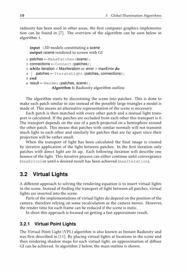
radiosity has been used in other areas, the first computer graphics implementa-tion can be found in [7]. The overview of the algorithm can be seen below inalgorithm 1.

input :3D models constituting a sceneoutput :scene rendered to screen with GI

1 patches←MakePatches(scene);2 connections←Connect(patches);3 while iteration < MaxIteration or error > maxError do4 patches←IterateLight(patches, connections);5 end6 result←Render(patches, scene);

Algorithm 1: Radiosity algorithm outline

The algorithm starts by discretizing the scene into patches. This is done tomake each patch similar in size instead of the possibly large triangles a model ismade of. This means an alternative representation of the scene is necessary.

Each patch is then matched with every other patch and a mutual light trans-port is calculated. If the patches are occluded from each other this transport is 0.The transport depends on the size of a patch projected on a hemisphere aroundthe other patch. This means that patches with similar normals will not transmitmuch light to each other and similarly for patches that are far apart since theirprojection will be rather small.

When the transport of light has been calculated the final image is createdby iterative application of the light between patches. In the first iteration onlypatches with direct light are lit up. Each following iteration will describe onebounce of the light. This iterative process can either continue until convergeance(maxError) or until a desired result has been achieved (maxIteration).

3.2 Virtual Lights

A different approach to solving the rendering equation is to insert virtual lightsin the scene. Instead of finding the transport of light between all patches, virtuallights are inserted into the scene.

Parts of the implementations of virtual lights do depend on the position of thecamera, therefore relying on some recalculation as the camera moves. However,the render time for each frame can be reduced if the scene is static.

In short this approach is focused on getting a fast approximate result.

3.2.1 Virtual Point Lights

The Virtual Point Light (VPL) algorithm is also known as Instant Radiosity andwas first described in [11]. By placing virtual lights at locations in the scene andthen rendering shadow maps for each virtual light, an approximation of diffuseGI can be achieved. In algorithm 2 below, the main outline is shown.

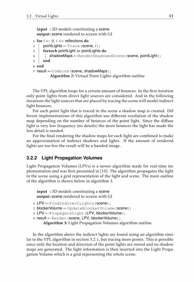
3.2 Virtual Lights 11

input :3D models constituting a sceneoutput :scene rendered to screen with GI

1 for i ← 0, i <= reflections do2 pointLights←Trace(scene, i);3 foreach pointLight in pointLights do4 shadowMaps←RenderShadowedScene(scene, pointLight);5 end6 end7 result←Combine(scene, shadowMaps);

Algorithm 2: Virtual Point Lights algorithm outline

The VPL algorithm loops for a certain amount of bounces. In the first iterationonly point lights from direct light sources are considered. And in the followingiterations the light sources that are placed by tracing the scene will model indirectlight bounces.

For each point light that is traced in the scene a shadow map is created. Dif-ferent implementations of this algorithm use different resolution of the shadowmap depending on the number of bounces of the point light. Since the diffuselight is very low frequency (no details) the more bounces the light has made theless detail is needed.

For the final rendering the shadow maps for each light are combined to makean approximation of indirect shadows and lights. If the amount of renderedlights are too few the result will be a banded image.

3.2.2 Light Propagation Volumes

Light Propagation Volumes (LPVs) is a newer algorithm made for real-time im-plementation and was first presented in [10]. The algorithm propagates the lightin the scene using a grid representation of the light and scene. The main outlineof the algorithm is shown below in algorithm 3.

input :3D models constituting a sceneoutput :scene rendered to screen with GI

1 LPV←FindIndirectLights(scene);2 blockerVolume←UpdateBlockerVolume(scene);3 LPV←PropagateLight(LPV, blockerVolume);4 result←Render(scene, LPV, blockerVolume);

Algorithm 3: Light Propagation Volumes algorithm outline

In the algorithm above the indirect lights are found using an algorithm simi-lar to the VPL algorithm in section 3.2.1, but tracing more points. This is possiblesince only the location and direction of the point lights are stored and no shadowmaps are generated. The light information is then inserted into the Light Propa-gation Volume which is a grid representing the whole scene.

12 3 Global Illumination Algorithms

To represent the occluders of light, a second grid is created which is offset byhalf a grid from the light volume. This grid contains information about the scenegeometry and which grid positions are occupied and not. To keep it dynamic andreal time, the grid is automatically updated with information from the camera.The drawback is that geometry that is occluded from the camera (or has not beenlooked at) is not used in light calculations.

When blocking geometry and initial light has been calculated the LPV is up-dated by propagating the light in the volume. The light propagation is blockedby the geometry if necessary.

The rendering of the scene samples the resulting LPV to get an estimation ofthe indirect light in the scene. This volume can also be used for participatingmedia effects by ray tracing.

3.3 Tracing Algorithms

The most popular approach to solving the rendering equation is by different trac-ing algorithms. These algorithms use paths, photons or cones to trace informa-tion about what light is likely to hit a certain surface or where light from a sourceshould be applied to the scene. Tracing algorithms rely on performing a lot oftraces to get an accurate result. They can also use approximations of either thedistribution of light or the representation of the scene to get a better result withless traces.

This type of algorithm relies heavily on the location of the camera for most ofthe calculations. The traces are usually optimized to only consider paths that areseen by the camera to get results faster.

In short this approach is focused on getting an accurate answer by brute force(with some approximations).

3.3.1 Path Tracing

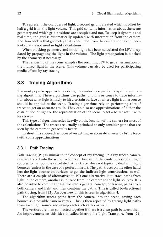
Path Tracing (PT) is similar to the concept of ray tracing. In a ray tracer, camerarays are traced into the scene. When a surface is hit, the contribution of all lightsources to that point is calculated. A ray tracer does not typically deal with lightbounces (unless in the case of a perfect mirror). The path tracer on the other handlets the light bounce on surfaces to get the indirect light contributions as well.There are a couple of alternatives to PT; one alternative is to trace paths fromlight to the camera; another is to trace from the camera to the light sources. It isalso possible to combine these two into a general concept of tracing paths fromboth camera and light and then combine the paths. This is called bi-directionalpath tracing, from [12]. An overview of this is seen in algorithm 4.

The algorithm traces paths from the camera into the scene, saving eachbounce as a possible camera vertex. This is then repeated by tracing light pathsfrom each light source and saving each such vertex as well.

The vertices are then connected together if there is a clear path between them.An improvement on this idea is called Metropolis Light Transport, from [21],

3.3 Tracing Algorithms 13

input :3D models constituting a sceneoutput :scene rendered to screen with GI

1 cameraVertices←TraceCamera(scene);2 lightVertices←TraceLights(scene);3 paths←Connect(lightVertices, cameraVertices);4 result←CalculateContributions(paths);

Algorithm 4: Bi-directional path tracing algorithm outline

which mutates the paths and saves the ones that contribute the most to the result.This alteration creates a better result faster, especially in scenes with narrow pas-sages for the light.

When the paths have been established the result is rendered taking the contri-bution to each pixel from the paths it is connected to. To get a good result, a lotof paths are needed which takes a lot of time to calculate.

3.3.2 Photon Mapping

Photon Mapping (PM) traces photons from each light source and places themin the scene. The photons density for each pixel is then sampled to render thescene. The algorithm was first introduced in [8] and an outline is seen below inalgorithm 5.

input :3D models constituting a sceneoutput :scene rendered to screen with GI

1 photonMap←TracePhotons(scene);2 result←Sample(photonMap);

Algorithm 5: Photon mapping algorithm outline

The algorithm starts by tracing photons from each light source into the scene.The photons can either be absorbed, reflected or transmitted when hitting a sur-face. When a photon is absorbed it is saved to the photon map of the scene. Thisacts as a density map of photons in the scene, storing positions, directions andcolors of the photons that have been traced.

To render the resulting scene the photon map is sampled for the closest pho-tons for each pixel. Then an estimation of the incoming light in that point iscreated, which is used to color the final pixel value.

3.3.3 Voxel Cone Tracing

Voxel Cone Tracing (VCT) was first described by [3] and [20]. It calculates an ap-proximation of the indirect light in a rendered scene using a voxel representationof the scene. The voxel representation makes it possible to sample the scene inreal-time. The outline is shown below in algorithm 6.

The algorithm starts by creating the voxel representation. There are severalapproaches for voxelizing a scene. In [3] the rendering pipeline is used to create

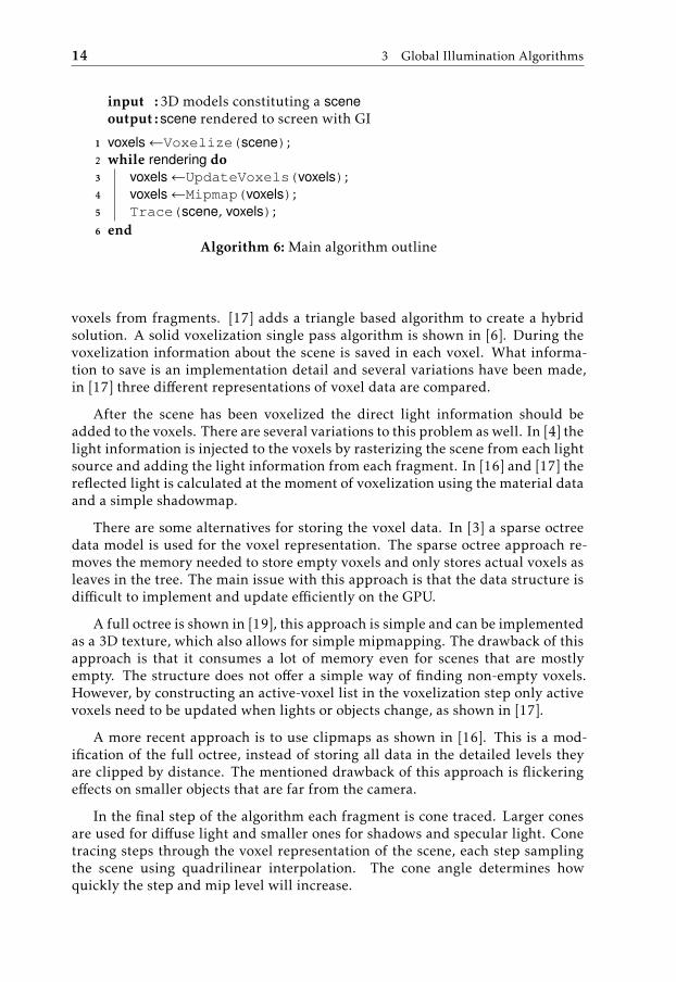
14 3 Global Illumination Algorithms

input :3D models constituting a sceneoutput :scene rendered to screen with GI

1 voxels←Voxelize(scene);2 while rendering do3 voxels←UpdateVoxels(voxels);4 voxels←Mipmap(voxels);5 Trace(scene, voxels);6 end

Algorithm 6: Main algorithm outline

voxels from fragments. [17] adds a triangle based algorithm to create a hybridsolution. A solid voxelization single pass algorithm is shown in [6]. During thevoxelization information about the scene is saved in each voxel. What informa-tion to save is an implementation detail and several variations have been made,in [17] three different representations of voxel data are compared.

After the scene has been voxelized the direct light information should beadded to the voxels. There are several variations to this problem as well. In [4] thelight information is injected to the voxels by rasterizing the scene from each lightsource and adding the light information from each fragment. In [16] and [17] thereflected light is calculated at the moment of voxelization using the material dataand a simple shadowmap.

There are some alternatives for storing the voxel data. In [3] a sparse octreedata model is used for the voxel representation. The sparse octree approach re-moves the memory needed to store empty voxels and only stores actual voxels asleaves in the tree. The main issue with this approach is that the data structure isdifficult to implement and update efficiently on the GPU.

A full octree is shown in [19], this approach is simple and can be implementedas a 3D texture, which also allows for simple mipmapping. The drawback of thisapproach is that it consumes a lot of memory even for scenes that are mostlyempty. The structure does not offer a simple way of finding non-empty voxels.However, by constructing an active-voxel list in the voxelization step only activevoxels need to be updated when lights or objects change, as shown in [17].

A more recent approach is to use clipmaps as shown in [16]. This is a mod-ification of the full octree, instead of storing all data in the detailed levels theyare clipped by distance. The mentioned drawback of this approach is flickeringeffects on smaller objects that are far from the camera.

In the final step of the algorithm each fragment is cone traced. Larger conesare used for diffuse light and smaller ones for shadows and specular light. Conetracing steps through the voxel representation of the scene, each step samplingthe scene using quadrilinear interpolation. The cone angle determines howquickly the step and mip level will increase.

3.4 Conclusion 15

3.4 Conclusion

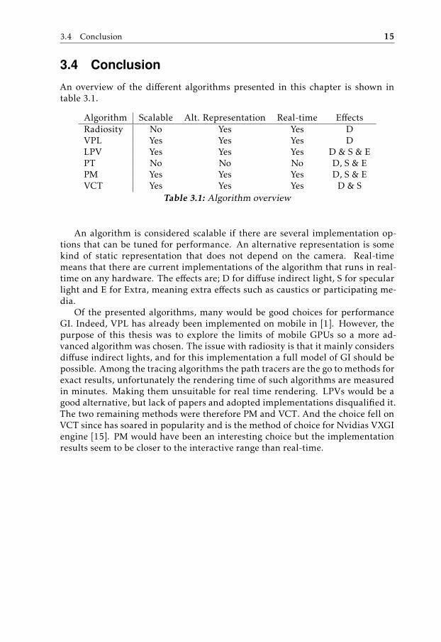
An overview of the different algorithms presented in this chapter is shown intable 3.1.

Algorithm Scalable Alt. Representation Real-time EffectsRadiosity No Yes Yes DVPL Yes Yes Yes DLPV Yes Yes Yes D & S & EPT No No No D, S & EPM Yes Yes Yes D, S & EVCT Yes Yes Yes D & S

Table 3.1: Algorithm overview

An algorithm is considered scalable if there are several implementation op-tions that can be tuned for performance. An alternative representation is somekind of static representation that does not depend on the camera. Real-timemeans that there are current implementations of the algorithm that runs in real-time on any hardware. The effects are; D for diffuse indirect light, S for specularlight and E for Extra, meaning extra effects such as caustics or participating me-dia.

Of the presented algorithms, many would be good choices for performanceGI. Indeed, VPL has already been implemented on mobile in [1]. However, thepurpose of this thesis was to explore the limits of mobile GPUs so a more ad-vanced algorithm was chosen. The issue with radiosity is that it mainly considersdiffuse indirect lights, and for this implementation a full model of GI should bepossible. Among the tracing algorithms the path tracers are the go to methods forexact results, unfortunately the rendering time of such algorithms are measuredin minutes. Making them unsuitable for real time rendering. LPVs would be agood alternative, but lack of papers and adopted implementations disqualified it.The two remaining methods were therefore PM and VCT. And the choice fell onVCT since has soared in popularity and is the method of choice for Nvidias VXGIengine [15]. PM would have been an interesting choice but the implementationresults seem to be closer to the interactive range than real-time.

4Implementation of Voxel Cone Tracing

The algorithm implemented and investigated in this work is VCT.

4.1 Overview

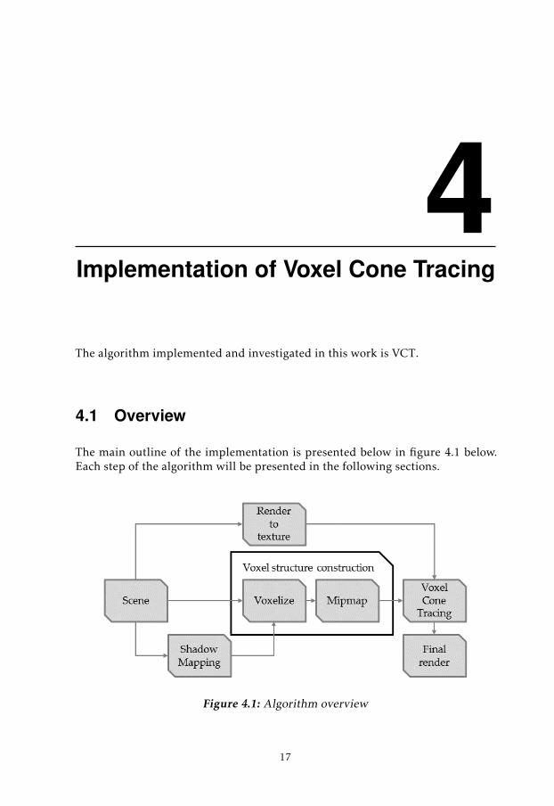
The main outline of the implementation is presented below in figure 4.1 below.Each step of the algorithm will be presented in the following sections.

Figure 4.1: Algorithm overview

17

18 4 Implementation of Voxel Cone Tracing

4.2 Shadow Mapping

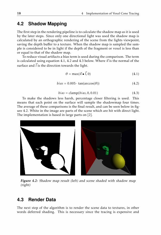
The first step in the rendering pipeline is to calculate the shadow map as it is usedby the later steps. Since only one directional light was used the shadow map iscalculated by an orthographic rendering of the scene from the lights viewpoint,saving the depth buffer to a texture. When the shadow map is sampled the sam-ple is considered to be in light if the depth of the fragment or voxel is less thanor equal to that of the shadow map.

To reduce visual artifacts a bias term is used during the comparison. The termis calculated using equation 4.1, 4.2 and 4.3 below. Where ~n is the normal of thesurface and ~l is the direction towards the light.

θ = max(~n •~l, 0) (4.1)

bias = 0.005 · tan(arccos(θ)) (4.2)

bias = clamp(bias, 0, 0.01) (4.3)

To make the shadows less harsh, percentage closer filtering is used. Thismeans that each point on the surface will sample the shadowmap four times.The average of these comparisons is the final result, and can be seen below in fig-ure 4.2. White in the image are parts of the scene which are hit with direct light.The implementation is based in large parts on [2].

Figure 4.2: Shadow map result (left) and scene shaded with shadow map(right)

4.3 Render Data

The next step of the algorithm is to render the scene data to textures, in otherwords deferred shading. This is necessary since the tracing is expensive and

4.4 Voxelization 19

should only be performed for pixels that are going to be displayed. The datathat is stored for each fragment is; albedo (diffuse color from texture or set color),position (in world coordinates), normals, tangents, bitangents (only on desktop),and depth. On mobile only four textures could be written in addition to the depthbuffer in one pass. This resulted in the bitangent being calculated in the shadersusing the normal and tangent, instead of rendering the scene a second time.

4.4 Voxelization

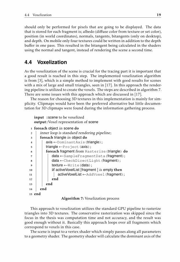
As the voxelization of the scene is crucial for the tracing part it is important thata good result is reached in this step. The implemented voxelization algorithmis from [3], which is a simple method to implement with good results for sceneswith a mix of large and small triangles, seen in [17]. In this approach the render-ing pipeline is utilized to create the voxels. The steps are described in algorithm 7.There are some issues with this approach which are discussed in [17].

The reason for choosing 3D textures in this implementation is mainly for sim-plicity. Clipmaps would have been the preferred alternative but little documen-tation for 3D clipmaps were found during the information gathering process.

input :scene to be voxelizedoutput :Voxel representation of scene

1 foreach object in scene do2 inner loop is standard rendering pipeline;3 foreach triangle in object do4 axis←DominantAxis(triangle);5 triangle←Project(axis);6 foreach fragment from Rasterize(triangle) do7 data←SampleFragmentData(fragment);8 data←CheckDirectLight(fragment);9 texture←Write(data);

10 if activeVoxelList [fragment ] is empty then11 activeVoxelList←AddVoxel(fragment);12 end13 end14 end15 end

Algorithm 7: Voxelization process

This approach to voxelization utilizes the standard GPU pipeline to rasterizetriangles into 3D textures. The conservative rasterization was skipped since thefocus in the thesis was computation time and not accuracy, and the result wasgood enough without it. Basically this approach loops over all fragments whichcorrespond to voxels in this case.

The scene is input to a vertex shader which simply passes along all parametersto a geometry shader. The geometry shader will calculate the dominant axis of the

20 4 Implementation of Voxel Cone Tracing

normal and will then project the input triangle along that axis for rasterization.In the fragment shader the fragment data, color and shadow map result, is usedto create a voxel (shown in 4.4.2. The count part of the voxel is set to eight,and the shadow map result is multiplied by eight. This is done so that the firstiteration of the mipmapping is not a special case. The voxel is then inserted intoa 3D texture using the fragment coordinates (x,y and z) as texture coordinates.The order they are used depends on the dominant axis.

An active voxel list is also created which contains the position of all voxelswhich are not empty along with the count of active voxels. The positions arestored in a 32 bit integer as a RB11G10. This allows for at least 1024 integerpositions in each dimension. This list is used both for mipmapping the 3D textureand also for rendering the voxels. It could also be used to update relevant partsof the texture in dynamic scenes.

4.4.1 Direct Light

In this implementation the direct light contribution is calculated during the vox-elization. The color of each voxel is calculated using equation 4.4.

colorvoxel = max(~n •~l, 0) · colordif f use (4.4)

The shadow map is then sampled to check if the fragment is hit with directlight.

This approach for direct light was chosen because it seemed to minimize thevisual artifacts in a simple and efficient way. It fit nicely in to the overall pipelineand the overhead of calculating the shadow map was low.

4.4.2 Data Storage

The final step in algorithm 7 is Write(data). In this implementation isotropicvoxels are used and the data saved is showed below in figure 4.3. The data isstored in a 3D texture. The reason for choosing isotropic voxels is that they aresimple to implement, require least amount of memory and has the best perfor-mance, as seen in [17].

Figure 4.3: Voxel data representation

To be able to use the necessary atomic operations all information has to bestored in a 32 bit integer texture. To make the most use of the data the bits areused as showed in figure4.3. The information that is saved for each voxel is theresult of the shadow map comparison and the color of the voxel. The order of thebits is important because voxelization uses the atomicMax operation to decide

4.5 Mipmapping 21

if a value should be overwritten or not. This ordering makes lit fragments moreimportant that unlit ones.

The reasoning behind the other bits is explained in the next section.

4.5 Mipmapping

The mipmap pipeline starts during the voxelization process by creating the firstlevel of the active voxel list. The active voxel list consists in part of an indirectdraw command buffer for each mipmap level, which is used for drawing onlythe non-empty voxels. The second part is an indirect compute command bufferfor each mipmap level, which can be used for compute shader operations on thevoxels, for example for creating all the mipmap levels in the 3D texture, as seenin algorithm 8.

input :VoxelList of base leveloutput :VoxelList for each mip level

1 foreach MipLevel do2 Each MipLevel has a corresponding VoxelList;3 foreach Voxel in VoxelList do4 VoxelNext←Combine(Voxel);5 end6 end

Algorithm 8: Mipmapping process

The compute shader goes through the active voxel list and uses it to calculatethe values for each voxel on the next level in the list. Since the data is saved ina 3D texture 8 voxels are used to create the data in the next level. The voxeldata from the current level is combined in the following way. Each voxel willatomically add data to the next voxel to maximize parallelization. For each voxelthe next level counter will increase by 1, the light counter will increase followingequation 4.5. The color of the next level voxel will increase by 1

8 of the colorvalue of the current voxel. This allows the sampling of the voxels to calculate theaverage, though some precision is lost.

lightnext =

1 if lightcurrent > countercurrent/20 otherwise

(4.5)

4.6 Voxel Cone Tracing

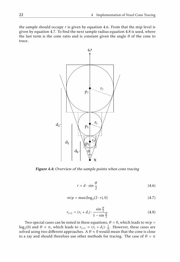
The final step of the rendering is the voxel cone tracing. The cone trace samplespoints from the voxel representation in increasingly higher mip levels. In fig-ure 4.4, a cone trace outline is shown. The trace starts at point x, in the directionω and begins by sampling at point p0, the distance d0 to the first sample point ischosen carefully to not intersect with the starting objects voxels. The radius that

22 4 Implementation of Voxel Cone Tracing

the sample should occupy r is given by equation 4.6. From that the mip level isgiven by equation 4.7. To find the next sample radius equation 4.8 is used, wherethe last term is the cone ratio and is constant given the angle θ of the cone totrace.

Figure 4.4: Overview of the sample points when cone tracing

r = d · sinθ2

(4.6)

mip = max(log2(2 · r), 0) (4.7)

ri+1 = (ri + di) ·sin θ

2

1 − sin θ2

(4.8)

Two special cases can be noted in these equations, θ = 0, which leads tomip =log2(0) and θ = π, which leads to ri+1 = (ri + di) · 1

0 . However, these cases aresolved using two different approaches. A θ ≈ 0 would mean that the cone is closeto a ray and should therefore use other methods for tracing. The case of θ = π

4.6 Voxel Cone Tracing 23

means that the cone covers the whole hemisphere, which would not give usefulresults. Instead to sample a larger angle, multiple cones with different directionsare used.

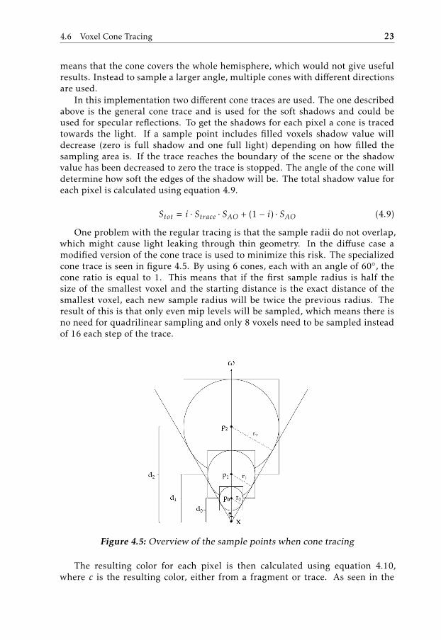
In this implementation two different cone traces are used. The one describedabove is the general cone trace and is used for the soft shadows and could beused for specular reflections. To get the shadows for each pixel a cone is tracedtowards the light. If a sample point includes filled voxels shadow value willdecrease (zero is full shadow and one full light) depending on how filled thesampling area is. If the trace reaches the boundary of the scene or the shadowvalue has been decreased to zero the trace is stopped. The angle of the cone willdetermine how soft the edges of the shadow will be. The total shadow value foreach pixel is calculated using equation 4.9.

Stot = i · Strace · SAO + (1 − i) · SAO (4.9)

One problem with the regular tracing is that the sample radii do not overlap,which might cause light leaking through thin geometry. In the diffuse case amodified version of the cone trace is used to minimize this risk. The specializedcone trace is seen in figure 4.5. By using 6 cones, each with an angle of 60, thecone ratio is equal to 1. This means that if the first sample radius is half thesize of the smallest voxel and the starting distance is the exact distance of thesmallest voxel, each new sample radius will be twice the previous radius. Theresult of this is that only even mip levels will be sampled, which means there isno need for quadrilinear sampling and only 8 voxels need to be sampled insteadof 16 each step of the trace.

Figure 4.5: Overview of the sample points when cone tracing

The resulting color for each pixel is then calculated using equation 4.10,where c is the resulting color, either from a fragment or trace. As seen in the

24 4 Implementation of Voxel Cone Tracing

equation, the result is only considering diffuse light, both when it comes to di-rect and indirect light. Multiplying the resulting diffuse trace with the color ofthe fragment is important to get realistic color interactions. A red indirect lightshould not color a green surface for example, this is an approximation of differentcolors being absorbed by different materials.

r = ~n •~l · Stot · clight · cf ragment + cdif f use · cf ragment (4.10)

The color of the trace is gathered in a similar way as the shadow value. Onlyduring this trace two separate values are filled; the accumulation of the result andthe color of the result. The color is determined by the average of the lit sampledvoxels. The accumulation increases regardless if the sampled voxel is lit or not.When the accumulation reaches one or if the boundary of the scene is reachedthe trace of the pixel is stopped.

4.7 Summary

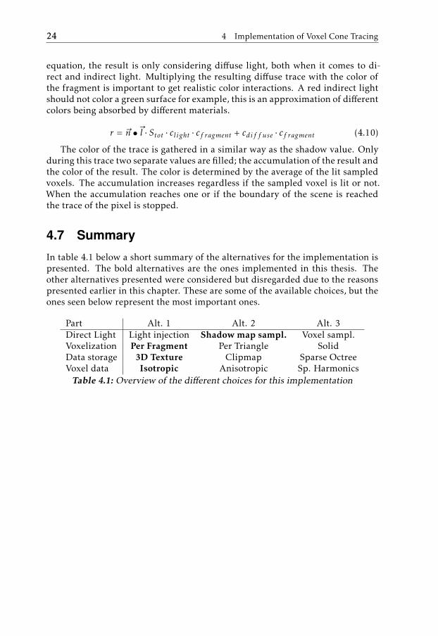
In table 4.1 below a short summary of the alternatives for the implementation ispresented. The bold alternatives are the ones implemented in this thesis. Theother alternatives presented were considered but disregarded due to the reasonspresented earlier in this chapter. These are some of the available choices, but theones seen below represent the most important ones.

Part Alt. 1 Alt. 2 Alt. 3Direct Light Light injection Shadow map sampl. Voxel sampl.Voxelization Per Fragment Per Triangle SolidData storage 3D Texture Clipmap Sparse OctreeVoxel data Isotropic Anisotropic Sp. HarmonicsTable 4.1: Overview of the different choices for this implementation

5Results

The implementation of the selected algorithm presented in the previous chapterresulted in a mobile implementation of VCT. It was also implemented on desk-top to compare the performance of the algorithm on different platforms and tocompare how much code could be re-used on the different platforms.

5.1 Comparisons

Five different scenes were rendered to compare the performance of the algorithmand show the increasing detail and realism added by the implemented algorithm.

5.1.1 Hardware

The algorithm was tested on the following hardware to compare the performanceof the implemented algorithm on a mobile, laptop and desktop GPU.

• Samsung Galaxy S7 Edge with Mali T880 MP12 GPU.

• Lenovo Y50 laptop with Nvidia GeForce GTX 860M GPU.

• Desktop with a Nvidia GeForce GTX 970 GPU.

Further specifications of the GPUs are shown below in table 5.1. An asteriskin the VRAM column signifies shared memory with the Central Processing Unit(CPU).

5.1.2 Timing method

To get the average times taken to render a frame, CPU timers together with theglFinish command was used. The glFinish commands made it possible to

25

26 5 Results

GPU Clock rate VRAM Cores L2 Cache GFLOPSMali T880 850 MHz 4 GB* 12 768 - 1536 kB 346.8Nvidia 860M 1020 MHz 2 GB, 6 GB* 640 2048 kB 1317.1Nvidia 970 1178 MHz 4 GB 1664 1792 kB 3494

Table 5.1: Hardware specifications

time individual steps for each frame by waiting for the command queue to ex-ecute. CPU timers were used because there are no GPU timers available forOpenGL ES 3.1, and using them on the other platforms could create skewed re-sults. Each scene was rendered for a number of frames before a frame averageover 5 frames was recorded. This was then repeated by restarting the program toget a fair average between multiple runs.

The Cornell box scene was run in multiple lighting conditions as follows.

• Scene 1: No GI

• Scene 2: No GI and shadowmapping

• Scene 3: AO and shadowmapping

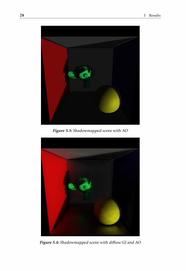
• Scene 4: Diffuse indirect light, AO and shadowmapping

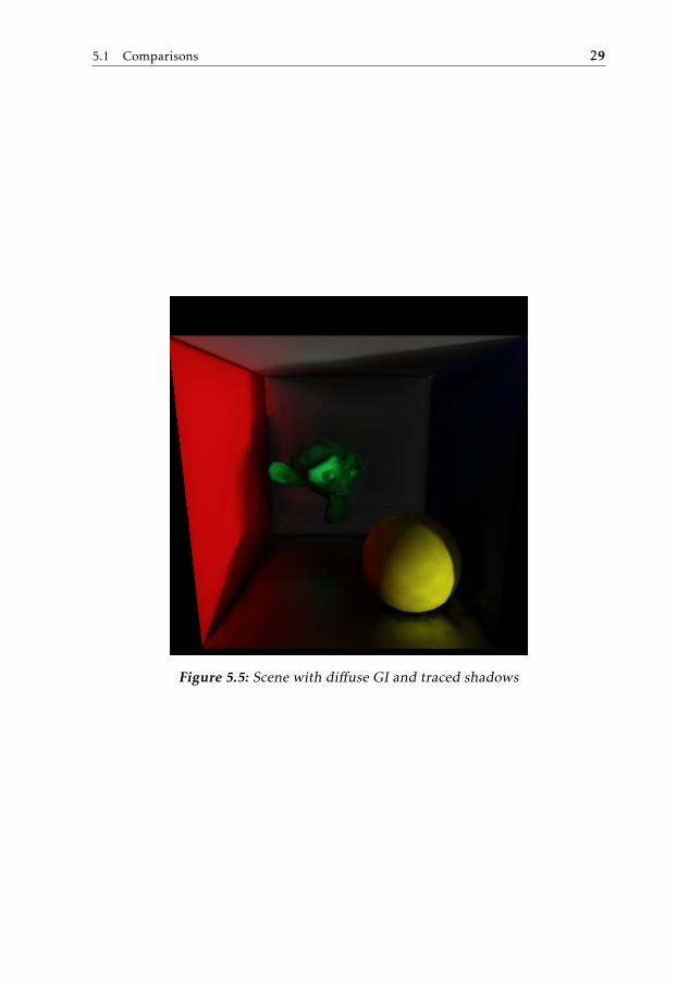
• Scene 5: Diffuse indirect light, AO and cone traced shadows

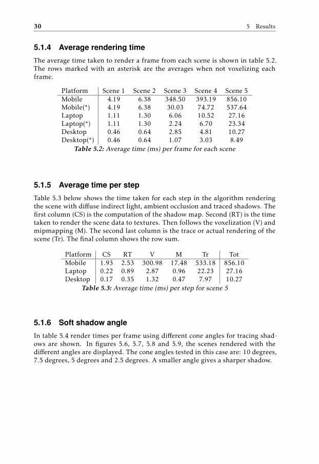
Each item in the list increases the performance and visual quality of the scene.

• In the first example the scene is shaded with a simple phong shader withboth diffuse and specular reflections of the global light.

• In the second example a shadowmap is added to increase the realism.

• In the third scene cone traced ambient occlusion is added.

• In the fourth scene a full diffuse bounce is added.

• In the fifth scene the shadowmap is replaced by cone traced shadows.

Each scene, unless otherwise stated, was tested with a resolution of 400x400pixels and used a voxel grid with 256x256x256 voxels. The traced shadow useda 5 degree angle and the shadow map resolution was 512x512 pixels.

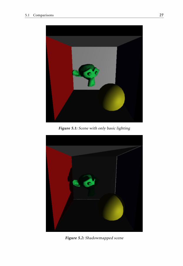
5.1.3 Visual comparison

The resulting images from mobile and desktop are shown below in figures 5.1,5.2, 5.3, 5.4 and 5.5.

5.1 Comparisons 27

Figure 5.1: Scene with only basic lighting

Figure 5.2: Shadowmapped scene

28 5 Results

Figure 5.3: Shadowmapped scene with AO

Figure 5.4: Shadowmapped scene with diffuse GI and AO

5.1 Comparisons 29

Figure 5.5: Scene with diffuse GI and traced shadows

30 5 Results

5.1.4 Average rendering time

The average time taken to render a frame from each scene is shown in table 5.2.The rows marked with an asterisk are the averages when not voxelizing eachframe.

Platform Scene 1 Scene 2 Scene 3 Scene 4 Scene 5Mobile 4.19 6.38 348.50 393.19 856.10Mobile(*) 4.19 6.38 30.03 74.72 537.64Laptop 1.11 1.30 6.06 10.52 27.16Laptop(*) 1.11 1.30 2.24 6.70 23.34Desktop 0.46 0.64 2.85 4.81 10.27Desktop(*) 0.46 0.64 1.07 3.03 8.49

Table 5.2: Average time (ms) per frame for each scene

5.1.5 Average time per step

Table 5.3 below shows the time taken for each step in the algorithm renderingthe scene with diffuse indirect light, ambient occlusion and traced shadows. Thefirst column (CS) is the computation of the shadow map. Second (RT) is the timetaken to render the scene data to textures. Then follows the voxelization (V) andmipmapping (M). The second last column is the trace or actual rendering of thescene (Tr). The final column shows the row sum.

Platform CS RT V M Tr TotMobile 1.93 2.53 300.98 17.48 533.18 856.10Laptop 0.22 0.89 2.87 0.96 22.23 27.16Desktop 0.17 0.35 1.32 0.47 7.97 10.27

Table 5.3: Average time (ms) per step for scene 5

5.1.6 Soft shadow angle

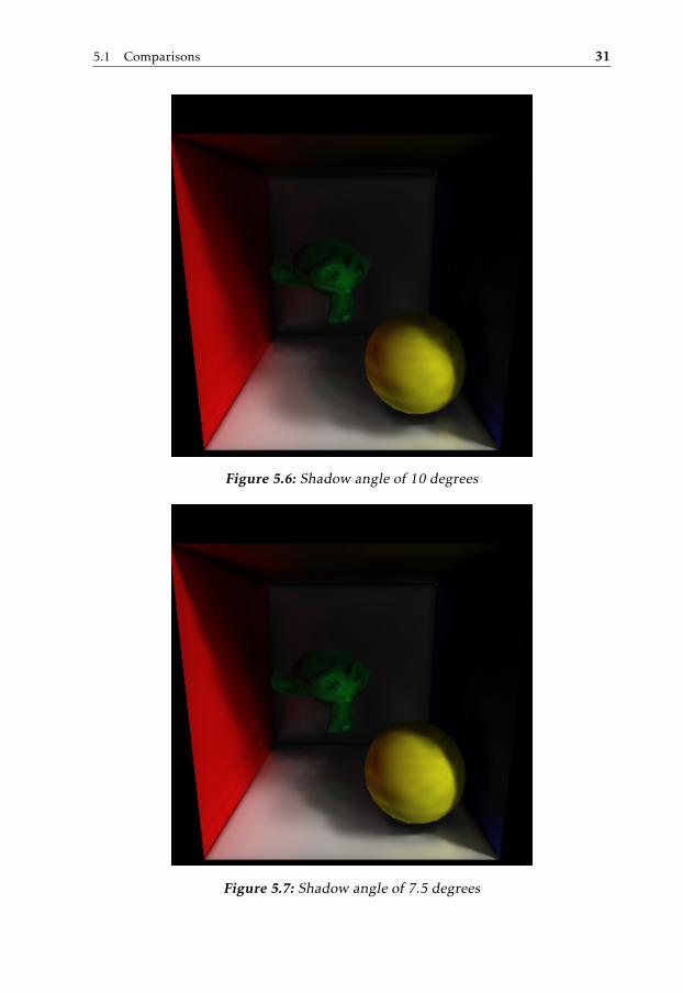
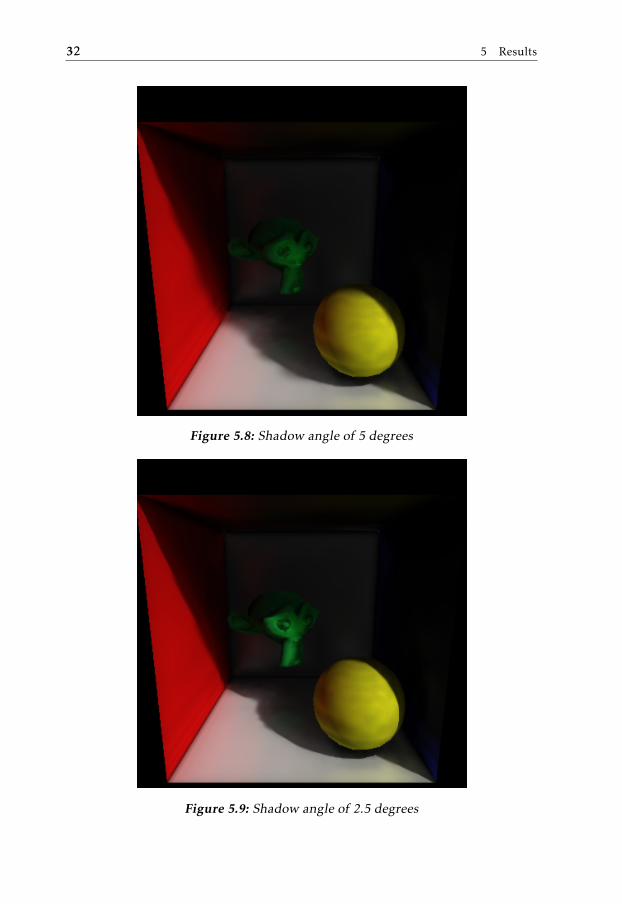
In table 5.4 render times per frame using different cone angles for tracing shad-ows are shown. In figures 5.6, 5.7, 5.8 and 5.9, the scenes rendered with thedifferent angles are displayed. The cone angles tested in this case are: 10 degrees,7.5 degrees, 5 degrees and 2.5 degrees. A smaller angle gives a sharper shadow.

5.1 Comparisons 31

Figure 5.6: Shadow angle of 10 degrees

Figure 5.7: Shadow angle of 7.5 degrees

32 5 Results

Figure 5.8: Shadow angle of 5 degrees

Figure 5.9: Shadow angle of 2.5 degrees

5.1 Comparisons 33

Platform 10 degrees 7.5 degrees 5 degrees 2.5 degreesMobile 291.57 378.04 536.82 1076.49Laptop 14.37 17.11 22.68 38.31Desktop 4.95 5.88 7.78 12.50

Table 5.4: Average time (ms) per frame for different angles during shadowtracing

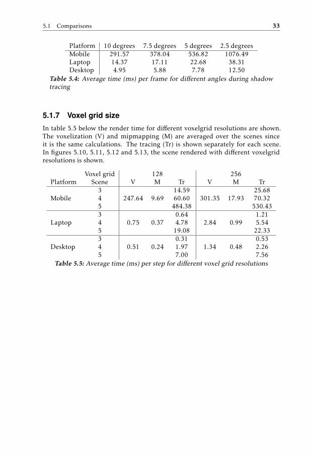
5.1.7 Voxel grid size

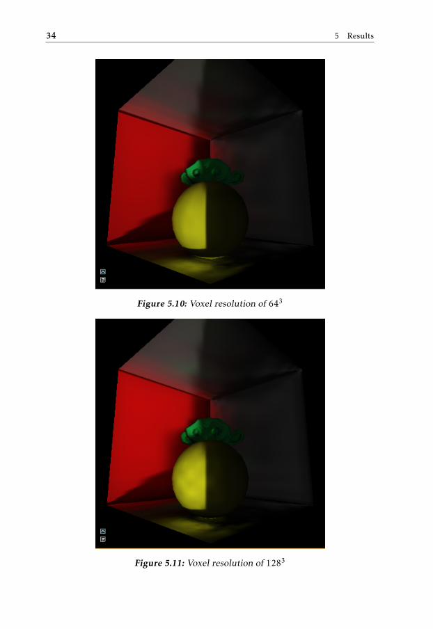
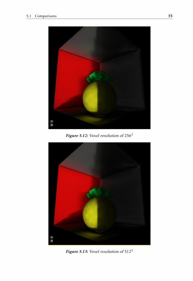
In table 5.5 below the render time for different voxelgrid resolutions are shown.The voxelization (V) and mipmapping (M) are averaged over the scenes sinceit is the same calculations. The tracing (Tr) is shown separately for each scene.In figures 5.10, 5.11, 5.12 and 5.13, the scene rendered with different voxelgridresolutions is shown.

Voxel grid 128 256Platform Scene V M Tr V M Tr

Mobile3

247.64 9.6914.59

301.35 17.9325.68

4 60.60 70.325 484.38 530.43

Laptop3

0.75 0.370.64

2.84 0.991.21

4 4.78 5.545 19.08 22.33

Desktop3

0.51 0.240.31

1.34 0.480.53

4 1.97 2.265 7.00 7.56

Table 5.5: Average time (ms) per step for different voxel grid resolutions

34 5 Results

Figure 5.10: Voxel resolution of 643

Figure 5.11: Voxel resolution of 1283

5.1 Comparisons 35

Figure 5.12: Voxel resolution of 2563

Figure 5.13: Voxel resolution of 5123

36 5 Results

5.2 Analysis

The results from the mobile and desktop show the same final rendering of thescene. The performance difference is clear between the different platforms, andthough most of the results do not show a real time solution on mobile, the AOdoes run on real time frame rates.

5.2.1 Image comparison

As seen in the images in figures 5.1 to 5.5 the realism of the rendering increasesfor each image. The first image contains no spatial information, only the directionof the light can be gathered from looking at the image. The next scene adds directshadows which gives some information about where the objects are located. Inscene 3 the AO adds locality by shading areas that are close, like the corners andunder the ball. In the fourth scene the indirect light is added which adds light toplaces that were previously unlit. In the final scene the soft shadows are added.

5.2.2 Average rendering time

Looking at table 5.2, it is clear that the overhead from voxelizing the scene eachframe is significant, especially for the mobile platform. All scenes, both with andwithout voxelization, reaches real time frame-rates on desktop and laptop. Formobile it is only achieved when calculating ambient occlusion without voxeliza-tion each frame.

From the table it is also clear that traced shadows adds a lot to the renderingtime of each frame, while there is less of a computational load to go from AO todiffuse indirect light.

5.2.3 Average time per step

As shown in table 5.3 the heaviest part of the algorithm is the cone tracing withinthe voxelized structure. The voxelization process, while taking a significant por-tion, still needs less time than the tracing. This is especially true for the desktopand laptop platforms where the ratio of time spent is dominated by the tracing.The mobile platform is more balanced between the voxelization and the tracing.

5.2.4 Soft shadows varying angle

The results of varying the shadow cone is shown to be significant in table 5.4, andas can be seen in figures 5.6 to 5.9 it has a clear effect on the result of the render-ing. Looking at table 5.4 and 5.3, it can be seen that the larger angles decreasethe time for cone tracing by enough to make it equal to the voxelization processon the mobile platform. The other platforms perform better on the voxelizationeven with a angle of 10 degrees.

5.3 Future Work 37

5.2.5 Voxel grid size

The voxel grid resolution impacts the result of the voxelization, mipmappingand tracing as shown in figure 5.5. The voxelization and mipmapping increasenoticably while the tracing times are increased slightly. The resulting renderingsare shown in figures 5.10 to 5.13. There are some visual errors seen in the lowerresolution renders, namely the light leaking under the yellow ball. There is alsoa noticable difference in the quality of the shadow close to the red/white corner.The diffuse indirect light is more focused in the higher resolutions, which is seenunder the ball, but also on the red diffuse light.

5.3 Future Work

This work has a lot of areas to improve upon when it comes to performance. Themost interesting ideas that were not implemented are the following.

• Use 3D clipmaps instead of mipmaps.

• Use filled voxel representation.

• Use low resolution light rendering and extrapolate to high resolution modelrendering.

6Conclusions

The results from the previous chapter show that the implemented algorithm doesnot reach real time frame rates on mobile. However, the scalability of the algo-rithm result in real time AO. Even though most of the code is usable on bothmobile and desktop, there are some differences worth noting.

6.1 Experiments

The results of the experiments, as shown in the previous chapter, indicate thatthere is still more development required before real time GI is realistic on mobilehardware. The only applicable real-time use of the implemented algorithm wasthe AO. It might be possible with extensive optimization to realize diffuse indi-rect light as well. The tracing of shadows, and therefore also specular indirectlight, is a long way off. Using VCT on a mobile device for something like AOmight increase the visual quality compared to screen space AO, but it has a highcost in memory and does not work for dynamic objects.

The voxelization times on the mobile platform are high when compared to theother platforms. One reason for this might be that the only measurement on themobile platform was during the initial construction since the 3D texture couldnot be cleared. It is therefore difficult to say how the voxelization process wouldperform when done continuously. Unfortunately there is no clearTexture inthe next version of OpenGL ES (3.2) either. So a continuous voxelization has tobe implemented with Vulkan if at all possible. However, it is possible to voxelizethe scene each frame using a laptop or desktop. This also means that the voxelstructure is completely static on the mobile platform.

In [24] it is suggested that mipmapping is a bottleneck, but in this thesis it isdemonstrated that this is not the case. The active voxel list reduces the mipmap-ping to only those sections of the 3D texture which have voxels, which causes the

39

40 6 Conclusions

mipmapping to require less time than the actual voxelization. Another possibil-ity which was not explored in this thesis is the possibilities of using the activevoxel list to update light changes.

The choice of isotropic voxels were part because of the performance and mem-ory aspects but also to utilize the glGenerateMipmap command, which wouldhave been used instead of developing a mipmap solution. Unfortunately thatcommand did not work while working on this implementation and mipmappingwas done using the active voxel list instead.

6.1.1 Method

The different scenes used in the previous chapter were selected to highlight someimportant differences in visual quality and performance. The reason no specularbounce was demonstrated is because the same code was used to trace shadows,which gave a more distinct visual difference. Since it performs a similar functionthe performance difference would be insignificant.

Unfortunately there was no simple way of clearing a 3D texture in OpenGL ES3.1, which meant that the voxelization could not be dynamic without reallocatinga new texture each frame. This resulted in the timings for creating the voxelrepresentation being based on fewer measurements and more importantly themeasurements were taken on the first run of the function. This might skew theresult towards a slower time than expected because of extra initialization costs.

6.1.2 Improvements

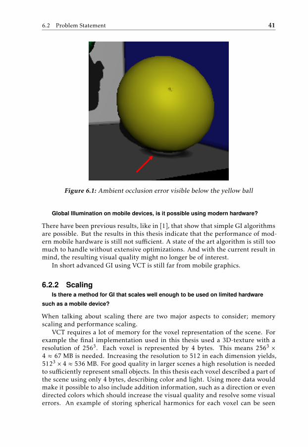
A problem with the voxel representation is that objects are empty inside. Thiscauses several minor problems. For example when tracing two nearby objects,the initial sampling offset might cause the first sample to be taken from insidethe hollow object. This causes the ambient occlusion tracing to fail, and the erroris easily seen. For example in figure 6.1, the shadow looks nice a bit away fromwhere the object touches the ground but closer to the contact point the shadowdisappears.

The empty voxel objects also cause problems with the mipmapping. Decidingif a certain voxel in the next resolution should be empty or filled must depend onthe existence of a single voxel, rather than deciding depending on the number ofavailable voxels. This might cause objects to grow too much in higher mip-levels.With filled objects, small objects would instead be removed in higher mip-levels.

6.2 Problem Statement

With the support of the experiments in the previous chapter the three questionsin the beginning of the thesis can be analyzed in more detail.

6.2.1 Possibility

6.2 Problem Statement 41

Figure 6.1: Ambient occlusion error visible below the yellow ball

Global Illumination on mobile devices, is it possible using modern hardware?

There have been previous results, like in [1], that show that simple GI algorithmsare possible. But the results in this thesis indicate that the performance of mod-ern mobile hardware is still not sufficient. A state of the art algorithm is still toomuch to handle without extensive optimizations. And with the current result inmind, the resulting visual quality might no longer be of interest.

In short advanced GI using VCT is still far from mobile graphics.

6.2.2 ScalingIs there a method for GI that scales well enough to be used on limited hardware

such as a mobile device?

When talking about scaling there are two major aspects to consider; memoryscaling and performance scaling.

VCT requires a lot of memory for the voxel representation of the scene. Forexample the final implementation used in this thesis used a 3D-texture with aresolution of 2563. Each voxel is represented by 4 bytes. This means 2563 ×4 ≈ 67 MB is needed. Increasing the resolution to 512 in each dimension yields,5123 × 4 ≈ 536 MB. For good quality in larger scenes a high resolution is neededto sufficiently represent small objects. In this thesis each voxel described a part ofthe scene using only 4 bytes, describing color and light. Using more data wouldmake it possible to also include addition information, such as a direction or evendirected colors which should increase the visual quality and resolve some visualerrors. An example of storing spherical harmonics for each voxel can be seen

42 6 Conclusions

in [17]. This means that the baseline for visual quality and memory is quite high,especially for larger scenes. Improvements such as clipmaps instead of mipmapshelp to reduce the memory footprint, but it consumes a lot of memory comparedto methods without alternative representations of the scene.

VCT is a tracing algorithm with little dependency between traces. But in thecase of cone tracing, each trace consist of many cones, looping over steps. Thiscan result in imbalanced workloads between threads. If the threads are grouped,like in the case of most GPUs, this leads to idle threads. Therefore, just scalingthe performance is not as effective.

To scale the performance of VCT there are other options. Resolution is animportant parameter that influences performance, since each pixel will result ina new trace, likely with a similar result. Two options to reduce this dependencyare:

• Grouping traces after a certain distance, like in [14].

• choosing pixels to trace and filter the result.

Resolution is of particular interest for mobile devices. High-end mobile de-vices usually come with high resolution screens, often higher than a laptop screen.Meaning that mobile devices come with a double disadvantage. First they havean equal or higher resolution than laptops and the GPU performance is less thanthat of a laptop.

Looking at the rendering time in table 5.2 and comparing that to the GFLOPSperformance of each GPU in table 5.1, the scaling between desktop and laptopcorresponds equally. The GFLOPS scaling, 3494

1317.1 ≈ 2.65, and the performancescaling (using scene 5, with voxelization), 27.16

10.27 ≈ 2.64. However comparing thedifference between desktop and mobile in GFLOPS, 3494

346.8 ≈ 10.07 with the per-formance in scene 4 (without voxelization), 74.72

3.03 ≈ 24.7, shows that the mobileperforms worse that what might be expected. Especially considering that thecores on the mobile phone are independent. One explanation for this might bethat the memory performance on mobile is slow, which would also explain whythe voxelization performs so poorly.

6.2.3 LimitsWhat are the limiting factors of the mobile device? And are there any potential

benefits on using mobile devices for Global Illumination?

The major limiting factor of the mobile device is the lack of performance of theGPU, which in turn is limited by power and size. A comparison of desktop andmobile GPUs in [13], also shows that there are different considerations that needto be made when implementing and optimizing algorithms. When it comes to theparticular algorithm implemented in this thesis, there are some potential bene-fits using mobile hardware for advanced computer graphics (that could possiblybe shown with more comprehensive experiments). Since the algorithm is com-pletely implemented on the GPU, moving data between CPU and GPU is not a

6.3 Mobile and desktop development 43

factor when it comes to performance, which in other cases can make a big differ-ence. As explained in the previous section the workload for threads in the sameworkgroup might be imbalanced, which can cause a problem on a GPU architec-ture that clusters multiple threads together (like most desktop GPUs). However,the mobile GPU used in this thesis has 12 independent cores meaning that thisshould not be a problem.

6.3 Mobile and desktop development

Developing for a mobile environment has both benefits and drawbacks comparedto desktop development. This section will discuss differences encountered dur-ing the work on this thesis.

6.3.1 OpenGL and OpenGL ES

While the overall thinking in OpenGL 3.0+ is nearly identical to OpenGL ES 2.0+there are differences to be aware of. Most differences deal with the often limitedhardware that OpenGL ES is targeted at. Developing a high-end algorithm in thisenvironment therefore had more limitations than just hardware.

Since OpenGL ES is aimed at low-performance hardware, many performancesettings are explicit. Selecting precision in shaders is an example of this, whichis something that is easy to forget coming from desktop OpenGL. This can causeerrors that are hard to find.

Since many of the advanced features from OpenGL 4.3+ are available inOpenGL ES 3.1+ it is surprising to find some of the simpler ones are not avail-able. For example the function clearTexture. The debug print tools doesnot appear until version 3.2 and neither does CLAMP_TO_BORDER for textures,which would have been useful to handle the case of a trace reaching the edge ofthe scene. Another feature missing is the ability to use subroutines in shadersinstead of relying on switch case statements.

6.3.2 Android

Developing for a mobile platform, the availability of third-party tools and codeis less frequent compared to desktop development. Especially when it comesto native development of GPU programming on mobile. Development for mo-bile devices is very specific for model and brand of the device which determinesOpenGL implementations and available features. Compared to bigger program-ming languages, Android NDK is not very commonly used which affects the pos-sibility to find answers to problems on Google and Stack Overflow. Just com-paring the android tag to android-ndk tag on Stack Overflow speaks of thedifference, over 900000 for android and just over 9700 for the android-ndk(October 2016). OpenGL is a bit closer with 27000 for opengl and 12000 foropengl-es. The NDK does allow more low level control which is necessary forcertain optimizations, but it is also more complicated and lacks many of the in-cluded help functions available when using higher level Java code.

44 6 Conclusions

Utilizing the very latest features may also cause some problems. The mobiledevice used was able to run OpenGL ES 3.2, which has some useful features.However, there were no libraries available which made it possible to compilecode for the newer API, since it was not part of the available version of Android.Also, no third-party solutions could be found.

6.3.3 Hardware

When developing for mobile it is not straight-forward to receive output and per-formance data. Especially not directly on the device. Even though current high-end mobile devices are powerful they are still not able to stand completely ontheir own. A laptop or desktop is still needed for debugging, tracing and out-put. Even though the screen has a high resolution there is no multi-tasking andbecause of the small physical size, text and input to be displayed is limited.

Another major difference is the lack of input methods for mobile devices. Ev-erything has to made for touch instead of mouse and keyboard. This makes itmuch more difficult to modify variables live and more difficult to navigate a 3Denvironment.

Development on specific hardware can be both helpful and problematic. Per-formance evaluation tools are usually available for most platforms, and Androidis no exception. However, the Android Studio performance tool required rootaccess which was not available at the time of writing, and seemed limited whenit came to OpenGL. Since the application used native C++ code and OpenGL,the number of tools available decreased. Many of the mobile GPU manufactur-ers have their own tools, which in the Mali case were very useful. However, theprofiling tool to measure performance of the application was not free and notdirectly available in a free version.

Bibliography

[1] Minsu Ahn, Inwoo Ha, Hyong-Euk Lee, and James D. K. Kim. Real-timeglobal illumination on mobile device. In Mobile Devices and Multimedia:Enabling Technologies, Algorithms, and Applications, volume 9030, pages903005–903005–5, 2014. Cited on pages 15 and 41.

[2] contact@opengl-tutorial.org. Shadow mapping tutorial.https://web.archive.org/web/20160818072411/http://www.opengl-tutorial.org/intermediate-tutorials/tutorial-16-shadow-mapping//, 2016. Accessed: 2016-10-27.Cited on page 18.

[3] Cyril Crassin and Simon Green. Octree-based sparse voxelization using thegpu hardware rasterizer. OpenGL Insights, pages 303–318, 2012. Cited onpages 13, 14, and 19.

[4] Cyril Crassin, Fabrice Neyret, Miguel Sainz, Simon Green, and Elmar Eise-mann. Interactive indirect illumination using voxel cone tracing. In Com-puter Graphics Forum, volume 30, pages 1921–1930. Wiley Online Library,2011. Cited on page 14.

[5] Cyril Crassin, David Luebke, Michael Mara, Morgan McGuire, Brent Oster,Peter Shirley, and Peter-Pike Sloan1 Chris Wyman. Cloudlight: A system foramortizing indirect lighting in real-time rendering. Journal of ComputerGraphics Techniques Vol, 4(4), 2015. Cited on page 2.

[6] Elmar Eisemann and Xavier Décoret. Single-pass gpu solid voxelization forreal-time applications. In Proceedings of Graphics Interface 2008, GI ’08,pages 73–80, Toronto, Ont., Canada, Canada, 2008. Canadian InformationProcessing Society. ISBN 978-1-56881-423-0. URL http://dl.acm.org/citation.cfm?id=1375714.1375728. Cited on page 14.

[7] Cindy M Goral, Kenneth E Torrance, Donald P Greenberg, and Bennett Bat-taile. Modeling the interaction of light between diffuse surfaces. In ACMSIGGRAPH Computer Graphics, volume 18, pages 213–222. ACM, 1984.Cited on page 10.

45

46 Bibliography

[8] Henrik Wann Jensen. Realistic image synthesis using photon mapping, vol-ume 364. Ak Peters Natick, 2001. Cited on page 13.

[9] James T Kajiya. The rendering equation. In ACM Siggraph ComputerGraphics, volume 20, pages 143–150. ACM, 1986. Cited on pages 1 and 6.

[10] Anton Kaplanyan and Carsten Dachsbacher. Cascaded light propagationvolumes for real-time indirect illumination. In Proceedings of the 2010ACM SIGGRAPH symposium on Interactive 3D Graphics and Games, pages99–107. ACM, 2010. Cited on page 11.

[11] Alexander Keller. Instant radiosity. In Proceedings of the 24th annualconference on Computer graphics and interactive techniques, pages 49–56.ACM Press/Addison-Wesley Publishing Co., 1997. Cited on page 10.

[12] Eric P Lafortune and Yves D Willems. Bi-directional path tracing. In Pro-ceedings of Third International Conference on Computational Graphics andVisualization Techniques (Compugraphics ’93), pages 145–153, 1993. Citedon page 12.

[13] Arian Maghazeh, Unmesh D Bordoloi, Petru Eles, and Zebo Peng. Generalpurpose computing on low-power embedded gpus: Has it come of age? InEmbedded Computer Systems: Architectures, Modeling, and Simulation(SAMOS XIII), 2013 International Conference on, pages 1–10. IEEE, 2013.Cited on page 42.

[14] James McLaren. Cascaded voxel cone tracing, 2014. CEDEC Presentation.Cited on page 42.

[15] Nvidia. Nvidia vxgi engine. https://web.archive.org/web/20160408115041/https://developer.nvidia.com/vxgi, 2016. Ac-cessed: 2016-11-07. Cited on page 15.

[16] Alexey Panteleev. Practical real-time voxel-based global illumination forcurrent GPUs, 2014. GTC Presentation. Cited on page 14.

[17] Randall Rauwendaal. Voxel based indirect illumination using spherical har-monics. PhD thesis, Oregon State University, 2013. Cited on pages 14, 19,20, and 42.

[18] Tobias Ritschel, Carsten Dachsbacher, Thorsten Grosch, and Jan Kautz. Thestate of the art in interactive global illumination. Comput. Graph. Forum,31(1):160–188, February 2012. ISSN 0167-7055. Cited on pages 2 and 9.

[19] Andrei Simion, Victor Asavei, Sorin Andrei Pistirica, and Ovidiu Poncea.Practical GPU and voxel-based indirect illumination for real time computergames. In 20th International Conference on Control Systems and ComputerScience (CSCS), pages 379–384. IEEE, 2015. Cited on page 14.

Bibliography 47

[20] Sinje Thiedemann, Niklas Henrich, Thorsten Grosch, and Stefan Müller.Voxel-based global illumination. In Symposium on Interactive 3D Graphicsand Games, pages 103–110. ACM, 2011. Cited on page 13.

[21] Eric Veach and Leonidas J Guibas. Metropolis light transport. In Proceed-ings of the 24th annual conference on Computer graphics and interactivetechniques, pages 65–76. ACM Press/Addison-Wesley Publishing Co., 1997.Cited on page 12.

[22] Conrad Wahlén. Desktop implentation source code. https://github.com/AnotherHermit/VoxelConeTracing, 2016. Accessed: 2016-11-12.Cited on page 3.

[23] Conrad Wahlén. Mobile implentation source code. https://github.com/AnotherHermit/VoxelConeTracingMobile, 2016. Accessed:2016-11-12. Cited on page 3.

[24] Oscar Westberg and Mikael Zackrisson. Voxel cone tracing. Technical report,Department of Electrical Engineering, Linköping University, 2016. Cited onpage 39.

[25] Gerald A Winer, Jane E Cottrell, Virginia Gregg, Jody S Fournier, and Lori ABica. Fundamentally misunderstanding visual perception: Adults’ belief invisual emissions. American Psychologist, 57:417, 2002. Cited on page 5.