Embed Size (px)
Citation preview

DPRIETI Discussion Paper Series 18-E-004
Global Sourcing and Domestic Production Networks
FURUSAWA TaijiHitotsubashi University
INUI TomohikoRIETI
ITO KeikoSenshu University
Heiwai TANGJohns Hopkins University
The Research Institute of Economy, Trade and Industryhttp://www.rieti.go.jp/en/
RIETI Discussion Paper Series 18-E-004 January 2018
Global Sourcing and Domestic Production Networks*
FURUSAWA
Taiji
Hitotsubashi U.
INUI
Tomohiko
Gakushuin U.
ITO
Keiko
Senshu U.
Heiwai TANG
Johns Hopkins and CESIfo
Abstract This paper studies how firms’ offshoring decisions shape a country’s domestic production networks. We develop a model in which heterogeneous firms source inputs from multiple industries located in different domestic regions and foreign countries. Input sourcing entails communication with suppliers, which is endogenously increasing in the differentiation of inputs. The model predicts that firms are less likely to source differentiated inputs, especially from distant domestic and foreign suppliers, due to costly communication. Triggered by foreign countries’ export supply shocks, firms start offshoring inputs from foreign suppliers, which displaces the less productive domestic suppliers in the same industry (the direct displacement effect). The resulting decline in marginal costs induces firms to start sourcing from the more productive and distant domestic suppliers within industries (within-industry restructuring effect), but possibly also from nearby suppliers that produce inputs that are more differentiated than those supplied by existing suppliers (the industry composition effect). The net effect of offshoring on a firm’s domestic production networks depends on the relative strength of the three effects, which we verify using data for 4.5 million buyer-seller links in Japan. Based on a firm-level instrument, we find that after offshoring, firms are less likely to drop suppliers on average, but more so for the larger ones. They tend to add nearby suppliers producing differentiated inputs. These results suggest that firms’ offshoring may increase the spatial concentration of domestic production networks.
Keywords: Production networks, Global sourcing, Offshoring, Face-to-face communication,
Industry agglomeration JEL codes: D22, D85, F14, L10, L14, R12
* The paper was previously circulated under the title “Offshoring, Relationship-Specificity, and Domestic Production Networks” (2015, RIETI Discussion Paper 15-E-122). The research is conducted as part of the Global Markets and Japan’s Industrial Growth project undertaken at the Research Institute of Economy, Trade and Industry (RIETI), and receives financial support from the JSPS KAKENHI Grants (No. 23243050, 26220503, 15K03456, and 16H03623). We thank the Ministry of Economy, Trade and Industry for providing the micro data of the Basic Survey of Japanese Business Structure and Activities, and RIETI for granting us access to the Tokyo Shoko Research data. We thank Pol Antràs, Andy Bernard, Matilde Bombardini, Masahisa Fujita, Yukiko Ito, Keith Head, Sam Kortum, Hiro Kasahara, Pravin Krishna, Masayuki Morikawa, Andreas Moxnes, Yukiko Saito, Tim Schmidt-Eisenlohr, Ya- suyuki Todo, Felix Tintelnot, Daniel Trefler, Jonathan Vogel, Ryuhei Wakasugi and participants at various seminars and conferences for comments. Tran Lam Anh Duong, Hiroki Ichimiya, Hayato Kato, and Kenji Suganuma provide excellent research assistance. All errors are our own.
1 Introduction
Substantial declines in trade barriers and advances in information, communication and transporta-
tion technologies have encouraged more firms to source inputs from far-away suppliers. A growing
body of literature studies both the causes and consequences of increasing global production frag-
mentation.1 The focus of the literature has been the direct effects of global sourcing on the industry
or firm that imports intermediate inputs, despite the fact that an economy is an interlinked web
of production units, each using inputs from its suppliers to produce goods and services that are
sold further downstream. Indeed, recent research has shown the significance of considering produc-
tion networks for a wide range of economic topics, such as the propagation and amplification of
firm-level shocks to large business-cycle fluctuations (Acemoglu et al., 2012; Carvalho and Gabaix,
2013); knowledge spillover (Javorcik, 2004); the aggregate effects of resource misallocation (Jones,
2011 and 2013); and the gains from trade (Costinot and Rodriguez-Clare, 2014; Caliendo and Parro,
2015). How global trade shapes the production networks in a country is an important yet relatively
under-explored topic.
This paper studies from both theoretical and empirical perspectives how firms’ sourcing of
intermediate inputs from foreign suppliers, which we refer to as offshoring, reshapes a country’s
domestic buyer-supplier networks. Specifically, we examine the effects of offshoring that is triggered
by foreign cost shocks on firms’choices of domestic input suppliers. To guide our empirical analysis,
we extend the global sourcing model by Antràs, Fort, and Tintelnot (2017, henceforth AFT) to
consider multiple domestic source regions, various input industries that differ in product differenti-
ation, and face-to-face communication between heterogeneous buyers and input suppliers. It builds
on the premise that trade is more costly over longer distance, and especially so when the success of
input production depends on the intensity of communication between buyers and suppliers. Similar
to Bernard, Moxnes, and Saito (2016, henceforth BMS), our model features heterogeneous buyers
and sellers engaged in costly domestic trade; but we additionally analyze firms’input sourcing from
both domestic and foreign suppliers in different input industries. We then empirically examine the
1See Feenstra (2008) for a comprehensive summary of the literature. Johnson and Noguera (2016) report thatthe ratio of value-added to gross exports worldwide declined by about 10 percentage points from 1970 to 2010,suggesting that production depended increasingly more on foreign inputs. Recent studies, which include Antràs,Fort, and Tintelnot (2017) and Blaum, Peters and Lelarge (2016) examine the productivity and welfare effects offirms’importing. There is also a large and growing literature about the effects of offshoring on labor market outcomes(e.g. Ebenstein, et al. 2014; Hummels et al., 2014).
2
theoretical predictions using Japanese extensive production network data.
There are at least three reasons why we extend the existing models of input sourcing to consider
multiple input industries and communication between buyers and sellers. First, from our Japanese
production network data, we observe that the geographic concentration of buyer-seller links is
higher for the more differentiated inputs, and is increasing over time. Second, we find that after
firms started to offshore inputs, they tend to expand the scope of domestic sourcing, especially
from the more proximate domestic suppliers, while cutting the ties with existing suppliers that
are large. A single-sector model that features only two-sided heterogeneity, standard trade costs,
and the scale effect of offshoring would predict the opposite patterns. Third, recent studies in
international trade and urban economics emphasize the role of information flows in shaping the
patterns of trade and city size distribution (e.g., Keller and Yeaple, 2013; Davis and Dingel, 2016;
Redding and Rossi-Hansberg, 2016).2 Studying the relationship between global sourcing and the
spatial distribution of economic activities in a country, in relation to information flow, is clearly
important.
Our model features variable trade costs increasing in distance not only because of the standard
transport costs but also buyers’costly communication with input suppliers. Face-to-face commu-
nication can help safeguard the quality of inputs, especially that of differentiated inputs. Buyers’
endogenous communication thereby raises the elasticity of the variable trade costs with respect
to distance from suppliers, more so for differentiated inputs. Therefore, to save communication
costs, buyers will choose to procure differentiated inputs from closer suppliers.3 Hence, in addition
to productivity sorting in outsourcing as documented in the literature (i.e., the more productive
firms self-select into a larger number of source regions, including the more distant domestic regions
and foreign countries),4 our multi-sector model illustrates a pecking order of firms’sourcing across
industries– firms are less likely to outsource differentiated inputs, especially from distant or foreign
suppliers.
After characterizing firms’equilibrium global production networks, we study how offshoring,
2Redding and Rossi-Hansberg (2016) provide a review of the extensive literature on the uneven spatial distributionof economic activities, due to exogenous geographic characteristics and endogenous interactions between agents.
3The idea that the agency costs of monitoring and communication increase in distance and shape relationship-specific investments has been empirically verified in the finance literature, such as Lerner (1995) and Petersen andRajan (2002). Cristea (2011) studies the importance of face-to-face meetings in shaping international trade and thedemand for business-class air travel.
4See Bernard et al. (2016) for a unified framework and a literature review.
3
triggered by exogenous increases in the attractiveness of offshoring, affects firms’performance and
thus their choices of domestic suppliers. Newly offshoring firms replace the less productive domestic
suppliers with foreign suppliers within the same industry (the direct displacement effect). The lower
marginal costs as a result of sourcing from more effi cient foreign suppliers, as highlighted by AFT,
induce firms to expand domestic sourcing by adding the more productive and distant suppliers,
while dropping the less productive and closer ones (the within-industry restructuring effect). If the
productivity effect is suffi ciently pronounced, newly offshoring firms may start paying extra fixed
costs to start sourcing in new input industries, which tend to be more differentiated (the industry
composition effect).
The net effect of offshoring on a firm’s structure of domestic suppliers is nuanced, as it depends
on the relative strength of the three effects of offshoring. In particular, offshoring tends to displace
generic-input suppliers, which were optimally chosen by buyers to be located farther away. Across
industries, newly offshoring firms tend to start sourcing differentiated inputs, which are associated
with high communication and thus variable trade costs. As such, to minimize communication
costs, newly offshoring firms choose domestic suppliers from the newly added differentiated input
industries that are closely located. These patterns of reorganization of supplier relationships may
overturn the within-industry restructuring effects, resulting in a paradoxical scenario in which firms
add closer and possibly smaller domestic suppliers and drop the more distant and possibly larger
ones after offshoring. The average distance from sellers in a buyer’s domestic production network
can drop after its offshoring, strengthening the spatial concentration of firms in related industries.
We empirically examine several theoretical predictions using data for 4.5 million buyer-seller
links in Japan.5 We find evidence largely consistent with BMS’s findings about Japan’s production
networks– the more productive firms source inputs from more suppliers and regions, including
the more distant ones. Distant suppliers are more productive on average, while productive firms
are more likely to offshore inputs. Above and beyond this spatial pattern of outsourcing, we
also uncover evidence that the negative correlation between distance and the scope of domestic
5The data set is the most comprehensive of all studies that we are aware of on domestic production networks.As will be discussed in Section 2, our network data set covers half of the registered firms in Japan, each of whichreports up to 24 suppliers and customers. We use the information reported by both buyers and sellers to maximizethe number of links. Recent research by Bernard, Moxnes and Saito (2016) and Carvalho et al. (2017) use the samenetwork data to study different research questions. The next closest counterpart that we can think of is the paper byAtalay et al. (2011), who analyze the buyer-seller network in the U.S. using Compustat data that cover only publiclylisted firms and their top 5 customers.
4
sourcing is stronger for the more differentiated inputs, as measured by the inverse of the elasticity
of substitution between input varieties. Hence, firms are less likely to source differentiated inputs
from the more distant regions or from foreign countries. Only the relatively more productive firms
will outsource differentiated inputs, with the most productive ones offshoring them.
Besides portraying the spatial and sectoral patterns of firms’global sourcing, we use the network
data to examine the model predictions about the effect of offshoring on firms’choices of domestic
suppliers. To establish the causal link between firms’offshoring and the pattern of domestic sourc-
ing, we construct a firm-level instrument using information on buyers’initial patterns of domestic
sourcing across industries and the corresponding foreign countries’export supply shocks. The idea
is that conditional on a firm’s sourcing inputs from a domestic input industry, the incremental fixed
costs needed for offshoring inputs in the same industry are lower. When positive export supply
shocks, due either to reduced trade costs or increased productivity of Japan’s trade partners, hit
an industry, those that are already sourcing inputs in the same industry should find offshoring
relatively more attractive.
The two-stage least squares estimates show that offshoring induces firms to add and drop larger
domestic suppliers simultaneously, while adding the more proximate ones. While the addition of
the larger suppliers is consistent with the within-industry restructuring effect of offshoring, both
dropping of the larger suppliers and adding of the closer suppliers need to be explained by the other
two effects. The dropping of the larger suppliers imply a suffi ciently strong direct displacement
effect, which is stronger in the less differentiated industries; while the adding of the more proximate
suppliers is due to the industry composition effect, which implies the addition of suppliers from
differentiated industries from which the buyers did not source inputs previously. Consistently, we
find that newly offshoring firms are more likely to start sourcing from the more differentiated input
industries. These results along with the higher likelihood of adding the more proximate suppliers
suggest a strong industry composition effect, and offer an explanation for why offshoring can reduce
the average distance between buyers and suppliers in production networks. The documented pat-
terns of supplier reorganization also have implications for analyzing how offshoring affects aggregate
productivity.6
6Such understanding is particularly important in light of Japanese firms’ increasing engagement in global valuechains. For instance, a Nikkei Sangyo Shimbun article on August 31, 2011 reported that Kubota Corporation, a largeindustry machinery manufacturing firm in Japan, announced the plan to increase its overseas parts and components
5
Our paper relates to several strands of literature. First, it contributes to the growing literature
on production networks and international trade. The study by Atalay, et al. (2011) is one of
the first in the literature to theoretically and empirically describe firms’production networks in a
country (the U.S.). Oberfield (2017) develops a model to study the endogenous formation of firms’
production networks and its impact on aggregate productivity. Thanks to the recently available
buyer-seller linked data, there is a burgeoning literature studying the pattern and dynamics of
domestic production networks.7 Notably, BMS use the same Japanese buyer-seller linked data to
highlight the negative assortativity of buyer-supplier links. Based on the extension of the high-
speed train line in Japan as an exogenous shock, the authors find that firms near newly built train
stations tend to increase sourcing from more domestic locations and thereby experience an increase
in measured productivity. Using the same data and exploiting the Great East Japan Earthquake
of 2011 as an exogenous shock, Carvalho et al. (2017) quantify the propagation of shocks through
the domestic input-output linkages.8 Tintelnot et al. (2017) develop and estimate a model of
firm-to-firm domestic trade, foreign trade, and endogenous network formation. Different from all
these studies, our paper focuses on characterizing both the industrial and geographic patterns of
domestic production networks. Importantly, we are the first to incorporate both domestic and
foreign sourcing in a model to empirically examine how firms’ offshoring shapes the domestic
production networks across sectors and space.
This paper also contributes to the growing cluster of work on networks in international trade.9
Recent research seeks to study the micro foundation of the dynamics and patterns of firms’sorting
and matching in international trade networks (e.g., Chaney, 2014; Eaton et al., 2014; Carballo,
Ottaviano, and Volpe Martincus, 2016; Bernard, Moxnes and Ulltveit-Moe, 2017; Sugita, Teshima,
and Seira, 2017).10 In particular, Bernard, Moxnes and Ulltveit-Moe (2017) build a model that fea-
procurement share form 25% in 2011 to 70% in 2021. A new overseas procurement base will be built in India, inaddition to their existing bases in Thailand and China. As part of this offshoring plan, the company would need toreorganize the procurement relationships with the existing domestic suppliers.
7Using U.S. buyer-seller linked data and a structural model of firms’network formation, Lim (2017) studies themacroeconomic implications of the propagation of firm-level demand and supply shocks through the productionnetworks.
8They show that external shocks on downstream firms affect not only the directly linked upstream firms, but alsofirms that are two or three degrees away from the affected firms.
9The literature dates back to the seminal work by Rauch (1999) and Rauch and Trindade (2002), who showthat colonial ties, common languages, and the stock of immigrants between two countries are positively related tobilateral trade, especially for differentiated products. The authors relate these findings to the importance of networks,information and search frictions in trade. See Chaney (2016) for a literature review.10Using importer-exporter matched data from Colombia, Eaton et al. (2014) structurally estimate the effects of
6
tures two-sided heterogeneity and uncover in Norwegian importer-exporter linked data the negative
assortative matching of trade partners.11 Chaney (2014) proposes theoretically that a country’s ag-
gregate export dynamics are tightly linked to firms’penetration into new foreign markets, through
establishing new contacts and expanding existing trade relationships. Different from this literature,
which focuses primarily on the patterns of importer-exporter matches, our paper focuses instead on
firm-to-firm relationships in the domestic economy, and investigates the impact of firms’offshoring
on the evolution of the domestic segment of global value chains.
Our work also contributes to the literature on the interplay between international trade and
the non-effi ciency aspect of firm performance. In particular, Holmes and Stevens (2014) find in the
U.S. manufacturing firm census data that small plants specialize in making specialty goods sold to
nearby customers, while large plants specialize in mass production of standardized goods shipped
to distant markets. Motivated by these facts, the authors structurally examine firms’heterogeneous
responses to import shocks from China, which cannot be explained by a standard heterogeneous-
firm model.12 Relatedly, we show paradoxically that large domestic suppliers are more likely to be
dropped, while proximate suppliers are more likely to be added, by the newly offshoring downstream
firms.13 In this regard, this paper shares similar key messages with Jensen and Kletzer (2005), who
study the tradability of tasks, and Keller and Yeaple (2013), who examine the ways multinationals
transfer knowledge to their overseas affi liates based on sector characteristics. In particular, we show
using firm-to-firm linked data that the elasticity of trade costs with respect to distance varies across
industries, and thus affects firms’reorganization of domestic production networks upon offshoring.
Finally, our paper relates to the large literature on the geography of trade and economic activities
(e.g., Ellison and Glaeser, 1997; Rosenthal and Strange, 2001; Dumais, Ellison, and Glaeser, 2002;
Ellison, Glaeser, and Kerr, 2010; and Nakajima, Saito, and Uesugi, 2012; Behrens and Bougna,
learning and search costs on aggregate trade. By focusing on a HS 6-digit code within textile/ apparel trade, Sugita,Teshima, and Seira (2017) study the rematching of US-Mexican trade relationships after the Multi-Fibre Arrangementquotas on Chinese exporters were removed in 2005. In a sample with mostly one-to-one matches, the authors findevidence of positive assortative matching in trade.11Similar to Carballo, Ottaviano, and Volpe Martincus (2016), the authors also highlight adjustments on the buyer
margin as an important channel through which trade responds to policy shocks.12 In particular, the authors find that large rather than small plants experience the largest contraction in sales in
response to the import shocks, in contrast to the predictions of a standard heterogeneous-firm model.13Another dimension of firm performance is product quality, which has been studied by a large and growing
literature, such as Khandelwal (2010), Baldwin and Harrigan (2011), and Hallak and Sivadasan (2013), amongothers.
7
2015),14 and the extensive literature on the impact of offshoring on labor market (Ebenstein et al.,
2014 and Hummels et al., 2014) and firm outcomes (Kasahara and Rodrigue, 2008; Hijzen, Inui,
and Todo, 2010; AFT, 2017).15 It contributes to the economic geography literature by showing
that offshoring can be a source of industry coagglomeration, as generic input suppliers, which
are on average located farther away, are the ones that tend to be displaced by foreign suppliers,
while differentiated input suppliers, which are on average located nearby, tend to be added as new
suppliers by offshoring firms. Contributing to the literature on the (direct) effects of offshoring,
our results about the patterns of supplier adding and dropping highlight a previously omitted
channel through which offshoring can affect an economy’s labor market outcomes and aggregate
productivity.
The paper proceeds as follows. Section 2 discusses the data sources. Section 3 presents several
stylized facts that motivate a theoretical model, which is introduced in Section 4. Section 5 discusses
our empirical design and findings. The final section concludes this paper.
2 Data
Our data come from two sources. The network data for 2005 and 2010 come from Tokyo Shoko
Research Ltd. (TSR), a private credit reporting agency. Firms provide information to TSR in order
to obtain credit scores for loans. The TSR data contain basic firm-level balance sheet information,
such as employment, sales, location, main (4-digit) industry (up to 3), founding year, number of
14Ellison and Glaeser (1997) propose sectoral measures of the degree of industry agglomeration and coagglom-eration, and find evidence of coagglomeration in industry pairs with strong upstream-downstream relationships.Rosenthal and Strange (2001) and Ellison, Glaeser, and Kerr (2010) empirically identify causes of agglomerationand coagglomeration, such as knowledge spillovers, input sharing, product shipping costs, labor market pooling, andnatural advantage. Rosenthal and Strange (2001) find that labor market pooling has the most robust effect, whileEllison, Glaeser, and Kerr (2010) find evidence that input-output linkages are particularly important. Using Japanesebuyer-seller linked data, Nakajima, Saito, and Uesugi (2012) find evidence that intensity of intra-industry transac-tions increases industry agglomeration. On the trends of industry agglomeration, Dumais et al. (2002) investigatedynamics of geographic concentration of U.S. manufacturing industries. They find that although the trend of indus-try agglomeration varies with industries, their average agglomeration levels have declined slightly in recent decades.Behrens and Bougna (2015) also observe a recent decline in the agglomeration of manufacturing plants in Canada.15Ebenstein et al. (2014) and Hummels et al. (2014) examine the effect of offshoring on workers’wages using U.S.
and Danish data, respectively. Kasahara and Rodrigue (2008) use Chilean manufacturing plant-level data and findthat firms’importing of intermediates improves productivity. Hijzen, Inui, and Todo (2010) find a positive impactof offshoring on Japanese firms’productivity. AFT build a multi-country sourcing model to study both theoreticallyand empirically firms’selection into importing and the resulting cost effects and complementarities between sourcingfrom different countries.
8

establishments, of over 800,000 firms in Japan.16 Crucially, it also provides information on firm-
to-firm relationships. Each firm surveyed by the TSR was asked to report the names of its top 24
suppliers, top 24 customers, and 3 main shareholders. To avoid the “top 24”cutoff from limiting
the sample coverage of the production network, we use a two-way matching method to maximize
the number of links, using information reported by a buyer about its sellers and vice versa. Since
a relationship with a buyer or seller can be reported by either end of a relationship, the number
of buyers (sellers) of a seller (buyer) can be much greater than 24. In fact, the top seller in our
constructed network data in Japan has over 11,000 buyers in 2010, while the top buyer has close to
8,000 suppliers. The distribution of the buyer-supplier links is very skewed, with most of the firms
having substantially fewer buyers and sellers (more below). Distance between any pair of buyers
and sellers is measured using the addresses reported by the firms, which we geocode.17
We complement the TSR data with the Basic Survey of Japanese Business Structure and Ac-
tivities (BSJBSA), conducted annually by the country’s Ministry of Economy, Trade and Industry
(METI). The BSJBSA data cover all firms that have over 50 employees or 30 million yen of paid-in
capital in the country’s manufacturing, mining, wholesale and retail, and several service sectors.
Firms’responses to the survey are mandatory. The survey data contain detailed information on
firms’business activities, such as their main industry (3-digit), number of employees, sales, capital
(which is required to compute a firm’s total factor productivity), purchases of inputs and mate-
rials, exports and imports by continent (e.g., Asia, Europe, etc.).18 The data set covers 22,939
and 24,892 firms for 2005 and 2010, respectively. We merge the two data sets using firms’names,
addresses, and telephone numbers. The merged data contain over 800,000 buyer-supplier pairs.19
In the regression analysis, we focus on the subsample that has manufacturing firms on the buyer
side of a relationship.
16The surveys were conducted in 2006 and 2011, respectively. We use both TSR Company Information Databaseand TSR Company Linkage Database in this paper. According to Carvalho et al. (2017), the TSR data cover morethan half of all firms in Japan. According to BMS, the TSR sample covers almost all firms with over 4 employees inJapan.17We use the geocoding service from the Center for Spatial Information Science at the University of Tokyo to first
identify the latitude and longitude of each address, and then compute the distance between any pair of coordinates.18The data set, however, does not provide information on firms’imports by sector.19About half of the observations of the balanced TSR sample have buyers that can be merged to firms included
in the manufacturing survey. See Table A3 in the appendix about the summary statistics of the key variables fromthe BSJBSA data. Importers’average imports-to-intermediate ratio, increases from 18% to 21% from 2005 to 2010.Asia is a very important input source for Japanese importers– among importers, the average share of imports fromAsia is over 80% in both 2005 and 2010.
9
3 Descriptive Evidence
3.1 Domestic Production Networks
We first describe several key patterns observed in our network data. Table 1 reports the summary
statistics on the buyer-supplier links. Panel A reports that the number of links, based on the TSR
sample, is about 3.6 millions in 2005 and 4.5 millions in 2010. The average number of sellers for a
buyer increased from 4.9 in 2005 to 5.5 in 2010, while the median increased from 2 to 3. The large
difference between the mean and the median numbers of sellers per buyer suggests a highly skewed
distribution of buyer-supplier links (i.e., a small number of large buyers have substantially more
sellers than other buyers).20 The increases in the average and median numbers of buyer-supplier
links since 2005 suggest that the production network in Japan is getting denser. Since the rise in
the density of the network may be due to firms’more comprehensive self-reporting of sellers, we
use a regression sample that includes only buyers and suppliers that operated in both 2005 and
2010, to mitigate this potential measurement issue.21
Panel B reports the summary statistics of the number of links in the regression sample built from
merging the BSJBSA firm sample with the TSR network data. Since BSJBSA imposes sampling
thresholds based on firms’employment and capital, the mean and the median numbers of sellers
linked to a buyer in our regression sample are larger (25 and 10, respectively, for the year 2005)
than those in the network data.22 Tables A1 and A2 in the appendix report more detailed statistics
by buyers’main industry.
Table 2 reports the summary statistics on the numbers of sellers and domestic regions (47
prefectures) from which different types of buyers, based on their import statuses, sourced inputs.
20When we plot the log number of sellers of a buyer against the fraction of buyers having at least that many sellers(Figure A1 in the appendix), we find a power-law distribution, as highlighted by BMS.21The cost of using a data set with balanced numbers of buyers and sellers in both years is that we cannot study
the entries and exits in the network.22One may be concerned about the selection biases arising from the exclusion of small firms in our regression
sample. Three remarks are in order. First, if the goal of the study is to evaluate the effects of firms’offshoring ontheir choices of domestic suppliers, the focus on large firms should be fine as large firms are more likely to engage inoffshoring, which entails high fixed costs (see AFT for the structural estimate of those fixed costs). Second, if there isany effect of offshoring on firms’performance and therefore their choices of domestic suppliers, omitting small firms,which tend to be non-importers, in our sample will go against us from finding any effect. It is because the variation infirms’participation in offshoring and the associated effects would have been even larger if small firms were includedin the sample. Third, even though the fraction of firms that have at least n links is naturally larger based on theregression sample, the power-law distribution of the number of sellers per buyer is preserved (see Figure A1 in theappendix). The slope of the relation based on the regression sample is almost identical to that derived from theoriginal TSR sample.
10
In 2005, there are altogether 13,784 manufacturing buyers in the regression sample. Of these buyers,
7% did not import in 2005 but started importing by 2010, while 74% continued to be non-importers
by 2010. Firms that imported in both 2005 and 2010 accounted for about 13% of the sample.23
These continuing importers sourced inputs from more domestic sellers and prefectures than new
importers and non-importers. They procured inputs from 48.5 domestic sellers in 2005 on average,
with the median equal to 16. The mean and median numbers of prefectures from which existing
importers procure inputs are 7.49 and 5, respectively. For new importers, while their numbers of
sellers and source prefectures are on average smaller than those of continuing importers, they are
larger than those of continuing non-importers.
Figures 1-3 illustrate the empirical regularities that discipline our theoretical model. Figure 1
shows that the number of buyer-seller links is negatively correlated with the distance between the
pair, and about half of the connections are observed within a 25 km radius of buyers. This negative
correlation appears to increase in magnitude since 2005. Figures 2 and 3 reveal the relationship
between a buyer’s sales and its scope of domestic sourcing. Figure 2 shows a positive correlation
between buyers’ sales and the number of connected domestic suppliers, while Figure 3 depicts
a positive correlation between their sales and the number of prefectures from which they source
inputs. We also find that within the same 4-digit industry and prefecture, the more productive
buyers use more suppliers, and distant suppliers tend to be more productive (see Table A4 in
the appendix for the regression results). These results altogether demonstrate the importance of
incorporating trade frictions that are increasing in distance, along with two-sided heterogeneity
across buyers and sellers in the model, similar to BMS.
3.2 Firms’Post-Offshoring Outcomes
Let us now present some preliminary empirical results about the correlation between a firm’s
offshoring (importing) status and its post-offshoring performance. We estimate the following spec-
ification using a simple fixed effects model:
∆yi = α+ β∆impi + γ lnTFPi + [FEs + FEr] + εi, (1)
23Notice that the shares of these firms do not add up to 1 as import stoppers are omitted in the table.
11
where ∆ is an operator that takes the first difference of the variable yi between 2005 and 2010, while
yi represents buyer i’s log sales or various measures of the scope of domestic sourcing, including log
numbers of domestic suppliers, domestic industries, and domestic regions respectively from which
buyer i sources inputs. We also examine how offshoring changes the average distance between a
buyer and its domestic suppliers. We use three measures of the change in a buyer’s average dis-
tance from its suppliers, represented by disti,t. The first one is the Davis-Haltiwanger-Schuh (1998)
growth rate of distance, (disti,10 − disti,05) /12 (disti,10 + disti,05), which is by construction bounded
between -2 and 2 to reduce the impact of outliers. The second measure is the log difference in the av-
erage distance. The third measure considers the difference between the average distance of the newly
added suppliers and that of the dropped suppliers,(distaddi − distdropi
)/1
2
(distaddi + distdropi
).
The variable of interest, ∆impi, represents the change in firm i’s import status, which equals 1
if buyer i did not import in 2005 but started to import in 2010, 0 otherwise.24 We include buyer’s
(4-digit) industry and region (prefecture) fixed effects (FEs and FEr) to control for any unobserved
determinants of firm outcomes (e.g., firms in certain prefectures are more likely to source inputs
due to a high geographic concentration of suppliers). We always control for buyer i’s 2005 log total
factor productivity, TFPi, as it is well documented in the literature that more productive firms are
more likely to import intermediate inputs (e.g., Amiti, Itskhoki, and Konings, 2014).
Table 3 reports the estimates of Equation (1). The regression sample includes manufacturing
buyers only, while the construction of a buyer’s performance measure uses information of its linked
suppliers in both manufacturing and non-manufacturing industries.25 Column 1 reports a positive
and significant correlation between the change in the firm’s import status and the change in its
sales. From columns 2 to 4, we find a positive and significant correlation between the change in
the firm’s import status and its scope of domestic sourcing, as measured by the (log) numbers of
suppliers, industries, or regions from which the firm sources its intermediate inputs.
In columns 5 and 6, we find a significant and negative correlation between a firm’s offshoring
24Recent research reveals that many exporters only export for a year and then drop out from exporting (e.g.,Blum, Claro, and Horstmann, 2013). To address the issues of occasional importing, we conduct robustness checks bydefining a new importer as one that imported for two consecutive years (2010 and 2011), and a non-importer as onethat did not import for three consecutive years (2003-2005). The main results remain robust and are available uponrequest.25When constructing the buyer-specific measures of domestic sourcing, we drop parent-child relationships and
sellers with fewer than 5 employees. The regression results remain largely robust when both data restrictions arerelaxed.
12
participation and the average distance between the firm and its domestic suppliers. In column 7, we
find that after a firm starts offshoring, the distance from the newly added suppliers relative to that of
the dropped suppliers tends to drop.26 Figures 4 and 5, which show the links of added and dropped
domestic suppliers of electronics firms that started offshoring inputs since 2005, portray a pattern
that suggests an increased geographic concentration of domestic production networks. Without
any causal implications, the results in Table 3 show insightful correlation between offshoring and
firms’domestic sourcing behavior. In Section 5, we will propose a firm-level instrument to gauge
the causal effect of offshoring on firms’adding and dropping of suppliers.
While the positive correlation between a firm’s import participation and the scope of domestic
sourcing is consistent with the main findings in AFT, the negative correlation between offshoring
and the average buyer-supplier distance cannot be readily rationalized by their model that only
considers a single input industry. We therefore develop our own model in the following section.
4 A Model of Firms’Global Sourcing
Motivated by the suggestive evidence above, we develop a model that features heterogeneous firms’
sourcing of intermediate inputs from suppliers located in different domestic and foreign regions.
4.1 Set-up
We consider a representative industry and build an industry equilibrium model that features global
sourcing (domestic sourcing and offshoring). Our model extends AFT to study the pattern of global
sourcing and the effect of offshoring on firms’domestic production networks. Similar to BMS, our
model considers input suppliers located in multiple domestic regions. Unlike their single-industry
models, however, we consider multiple input industries that differ in the degree of product differ-
entiation. We investigate how the differentiation of inputs changes firms’incentives to outsource
inputs and how offshoring affects firms’post-offshoring relationships with individual suppliers. We
also introduce in the model buyers’communication with sellers in an effort to enhance input quality
to show that the elasticity of trade costs with respect to distance can endogenously increase with
the differentiation of inputs. We first characterize firms’spatial and sectoral equilibrium patterns of
26The number of observations in column 7 is significantly smaller because not all buyers added or dropped sellersduring the sample period.
13
global sourcing, before examining the effect of a reduction in foreign input costs on buyers’choices
of domestic suppliers.
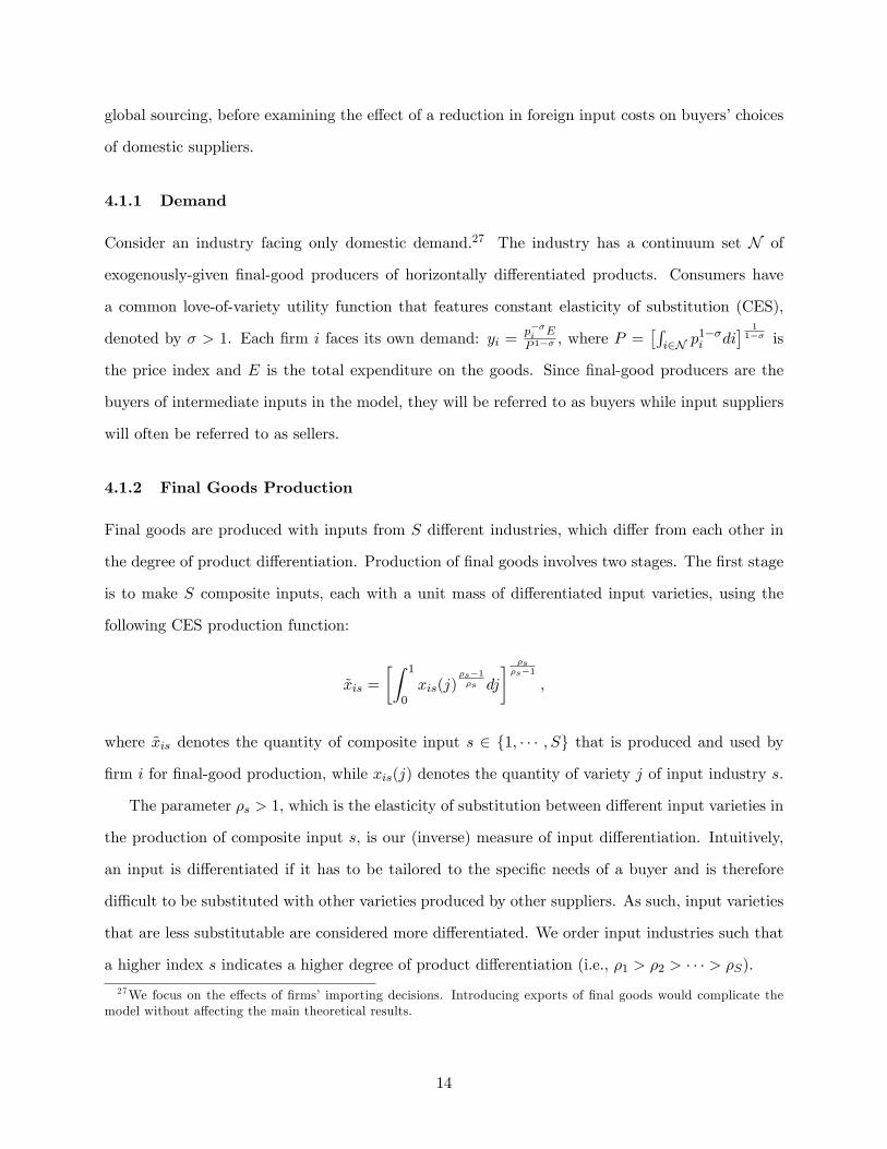
4.1.1 Demand
Consider an industry facing only domestic demand.27 The industry has a continuum set N of
exogenously-given final-good producers of horizontally differentiated products. Consumers have
a common love-of-variety utility function that features constant elasticity of substitution (CES),
denoted by σ > 1. Each firm i faces its own demand: yi =p−σi E
P 1−σ , where P =[∫i∈N p
1−σi di
] 11−σ is
the price index and E is the total expenditure on the goods. Since final-good producers are the
buyers of intermediate inputs in the model, they will be referred to as buyers while input suppliers
will often be referred to as sellers.
4.1.2 Final Goods Production
Final goods are produced with inputs from S different industries, which differ from each other in
the degree of product differentiation. Production of final goods involves two stages. The first stage
is to make S composite inputs, each with a unit mass of differentiated input varieties, using the
following CES production function:
xis =
[∫ 1
0xis(j)
ρs−1ρs dj
] ρsρs−1
,
where xis denotes the quantity of composite input s ∈ 1, · · · , S that is produced and used by
firm i for final-good production, while xis(j) denotes the quantity of variety j of input industry s.
The parameter ρs > 1, which is the elasticity of substitution between different input varieties in
the production of composite input s, is our (inverse) measure of input differentiation. Intuitively,
an input is differentiated if it has to be tailored to the specific needs of a buyer and is therefore
diffi cult to be substituted with other varieties produced by other suppliers. As such, input varieties
that are less substitutable are considered more differentiated. We order input industries such that
a higher index s indicates a higher degree of product differentiation (i.e., ρ1 > ρ2 > · · · > ρS).
27We focus on the effects of firms’ importing decisions. Introducing exports of final goods would complicate themodel without affecting the main theoretical results.
14
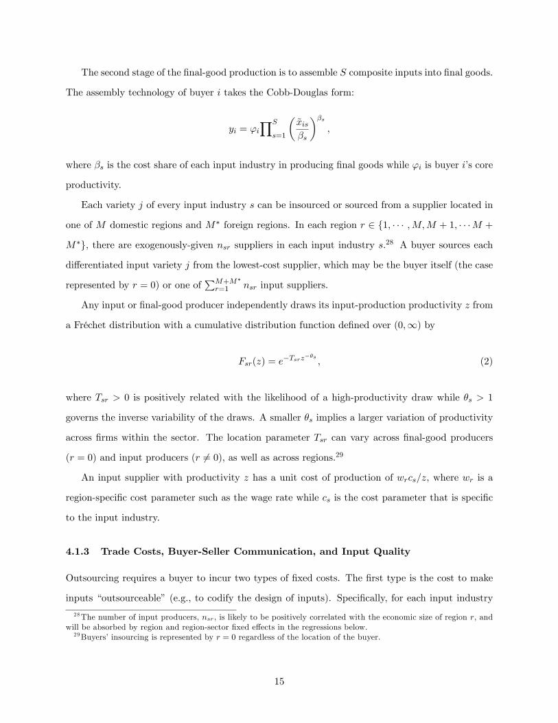
The second stage of the final-good production is to assemble S composite inputs into final goods.
The assembly technology of buyer i takes the Cobb-Douglas form:
yi = ϕi∏S
s=1
(xisβs
)βs,
where βs is the cost share of each input industry in producing final goods while ϕi is buyer i’s core
productivity.
Each variety j of every input industry s can be insourced or sourced from a supplier located in
one of M domestic regions and M∗ foreign regions. In each region r ∈ 1, · · · ,M,M + 1, · · ·M +
M∗, there are exogenously-given nsr suppliers in each input industry s.28 A buyer sources each
differentiated input variety j from the lowest-cost supplier, which may be the buyer itself (the case
represented by r = 0) or one of∑M+M∗
r=1 nsr input suppliers.
Any input or final-good producer independently draws its input-production productivity z from
a Fréchet distribution with a cumulative distribution function defined over (0,∞) by
Fsr(z) = e−Tsrz−θs
, (2)
where Tsr > 0 is positively related with the likelihood of a high-productivity draw while θs > 1
governs the inverse variability of the draws. A smaller θs implies a larger variation of productivity
across firms within the sector. The location parameter Tsr can vary across final-good producers
(r = 0) and input producers (r 6= 0), as well as across regions.29
An input supplier with productivity z has a unit cost of production of wrcs/z, where wr is a
region-specific cost parameter such as the wage rate while cs is the cost parameter that is specific
to the input industry.
4.1.3 Trade Costs, Buyer-Seller Communication, and Input Quality
Outsourcing requires a buyer to incur two types of fixed costs. The first type is the cost to make
inputs “outsourceable” (e.g., to codify the design of inputs). Specifically, for each input industry
28The number of input producers, nsr, is likely to be positively correlated with the economic size of region r, andwill be absorbed by region and region-sector fixed effects in the regressions below.29Buyers’insourcing is represented by r = 0 regardless of the location of the buyer.
15
in which a buyer outsources intermediate inputs, it has to incur a fixed cost of f , which is common
across input industries. The second type of fixed costs are those related to search in a region for
the lowest-cost sellers of individual input varieties. Borrowing the insight from AFT, we assume
that for every region a buyer searches for input suppliers, it incurs an industry-specific fixed cost of
fs. Costly search implies that firms will not source inputs from all regions. Let Ωis denote the set
of regions from which firm i sources inputs in industry s. The set Ωis may be a proper subset of
1, · · · ,M,M + 1, · · · ,M +M∗. We assume that no fixed cost is required for insourcing, so that
a buyer will always insource a fraction of varieties even in the industries that it outsources inputs.
There are also standard iceberg transport costs for domestic and foreign trade of inputs. They
take the form ts(d) ≥ 1 and ts(0) = 1, where ts is an industry-specific increasing function of the
distance d between the buyer’s region and a seller’s region.
The transport cost, however, is not the only trade cost that increases with the distance between
buyers and sellers. Buyers need to communicate with sellers to make sure that they receive what
they want. The cost of face-to-face communication naturally increases with distance, and its benefit
clearly depends on the differentiation of the inputs that are traded.30 Consider a misunderstanding
between a pair of buyer and seller about the specification of a product (e.g., size, shape, and color).
Low-quality parts and components may reduce the quality of final products at the minimum, and
can jeopardize the entire production process in the extreme situation.31 Based on the presumption
that the failure of delivering high-quality inputs often arises from miscommunication or misunder-
standing between buyers and sellers, we assume that a buyer can reduce the probability of failure
by engaging in face-to-face communication more vigorously.32
More specifically, we assume that for each input variety j ∈ [0, 1] in industry s, a seller’s
products meet the buyer’s expected standard with probability q, and fail to meet the standard
with probability 1 − q. We further assume that in the latter case, all inputs produced by that
30Despite the substantial improvement in information and communication technologies, business travels did notappear to decrease (Liu, Scholnick, and Finn, 2017). A majority of executives surveyed by Harvard Business Review(2009) claimed that in-person meetings are essential for “sealing the deal”and maintaining long-term relationships.31Kremer (1993), in his seminal O-ring theory of development, provides several real-world examples about how
low-quality inputs can reduce product quality (e.g., garment) at the minimum, and can destroy the final goodscompletely (e.g., the explosion of the space shuttle Challenger when one of the thousands of the parts, the O-ring,malfunctioned).32Communication involves exchanging ideas about product designs, monitoring the sellers’production processes,
among others. There is an extensive literature about how the diffi culty of writing complete contracts can result inhold-up and ex-ante underinvestment by both firms. See Antràs (2015) for a book-length analysis of the topic.
16

seller are useless for the buyer. Buyers, however, can affect q by engaging in communication with
individual input suppliers, which raises the unit cost of shipped inputs by a multiple of em(d)q,
where m is an increasing function of the distance between the buyer and a seller.33 The marginal
communication cost rises with the distance (i.e., face-to-face communication with distant sellers is
more costly).
In this model, we assume for simplicity that buyers have all the bargaining power against input
suppliers, so that the price of an input equals its unit cost.34
Given a productivity distribution ϕii∈N , each buyer imakes a sequence of decisions as follows:
1. Buyer i as well as each input supplier draws its productivity for input production. Buyer i
knows its own productivities for input production for all j ∈ [0, 1] in every input industry
s = 1, · · · , S.
2. In every input industry s, buyer i chooses whether to outsource or not, and pays f for every
industry that it has chosen to outsource. In addition, for each industry s that it has chosen
to outsource, it selects a set of regions that it searches for input suppliers, and pays fs for
every such region.
3. For each input variety j ∈ [0, 1] of industry s that it has chosen to outsource, buyer i chooses
the lowest-price (inclusive of trade costs) supplier of all the input suppliers in regions in Ωis
and itself.
4. For each region r ∈ Ωis, buyer i chooses the optimal sector-specific intensity of communication
with the sellers.
5. Buyer i optimally sets its final-good price, which will be a constant mark-up over its marginal
cost.33By specifying the communication as a variable cost rather than a fixed cost, we assume that the intensity of
communication is increasing in the value of transaction. The finding of a positive correlation between the total valueof outsourcing and the number of business travels at the industry level for the U.S. offer indirect evidence for thatassumption (Liu, Scholnick, and Finn, 2017).34 Introducing explicit negotiation between buyers and sellers would not change the results qualitatively.
17
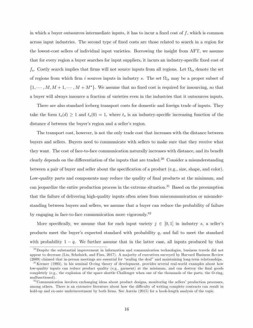
4.2 Optimal Communication Intensity
We now derive each firm i’s optimal communication intensity, characterized by the probability
q = qisr that firm i receives high-quality inputs, taking its set of source regions, ΩisSs=1, as given.
For a given set of suppliers in the regions in Ωis and hence a given set of prices for the input
varieties of industry s, buyer i chooses qisr to minimize the effective unit cost of the composite
input s. Let Gisr denote the probability distribution of the price of inputs sourced from region r.
Also let Iisr denote the set of inputs sourced from region r and µ(Iisr) its measure. Due to the law
of large numbers, the mass (1 − qisr)µ(Iisr) of the input varieties sourced from region r ∈ Ωis is
useless, while the prices of remaining qisrµ(Iisr) of input varieties are distributed according to the
distribution of Gisr. There is no such loss for insourced varieties.
Firm i optimally selects how much it purchases from each seller, given the risk of receiving
useless inputs with probability 1 − qisr. As shown in Appendix A, the resulting unit cost for the
composite input s, denoted by cis, reflects this risk:
cis =
µ(Iis0)
∫ ∞0
p1−ρsdGis0(p) +∑r∈Ωis
µ(Iisr)
∫ ∞0
(q
ρs1−ρsisr p
)1−ρsdGisr(p)
11−ρs
. (3)
Note that for r ∈ Ωis, unit cost p is multiplied by qρs
1−ρsisr > 1. This means that the complete loss
of a fraction 1 − qisr of the input varieties is equivalent to a uniform increase in the unit costs of
varieties by the multiple of qρs
1−ρsisr ; the smaller ρs (i.e., the higher the product differentiation), the
greater the increment of the cost, measured by qρs
1−ρsisr .
To alleviate the cost of receiving low-quality inputs, buyer i chooses qisr for each r ∈ Ωis to
minimize qρs
1−ρsisr p, which can be written as
qρs
1−ρsisr p = q
ρs1−ρsisr wrcsts(dir)e
m(dir)qisr/z,
where dir denotes the distance between buyer i and region r. It can be readily verified that the
cost-minimizing qisr is given by
qisr =ρs
(ρs − 1)m(dir). (4)
The communication intensity (or the probability of receiving high-quality inputs) and hence the
18
communication costs decrease with ρs and dir. Buyers have more incentive to enhance the commu-
nication with sellers of the more differentiated inputs, since failing to obtain high-quality inputs is
more costly due to a lower substitutability between input varieties. The communication incentive
diminishes with the distance to the supplier because face-to-face communication, by assumption,
is more costly over longer distance.
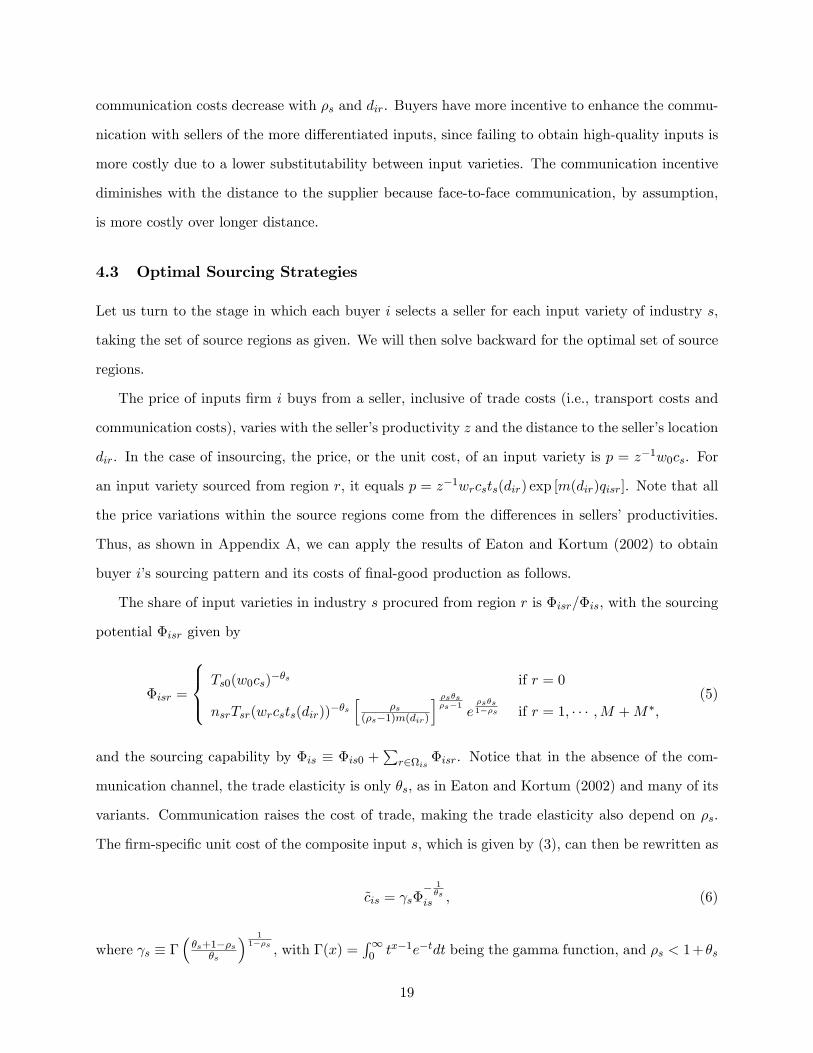
4.3 Optimal Sourcing Strategies
Let us turn to the stage in which each buyer i selects a seller for each input variety of industry s,
taking the set of source regions as given. We will then solve backward for the optimal set of source
regions.
The price of inputs firm i buys from a seller, inclusive of trade costs (i.e., transport costs and
communication costs), varies with the seller’s productivity z and the distance to the seller’s location
dir. In the case of insourcing, the price, or the unit cost, of an input variety is p = z−1w0cs. For
an input variety sourced from region r, it equals p = z−1wrcsts(dir) exp [m(dir)qisr]. Note that all
the price variations within the source regions come from the differences in sellers’productivities.
Thus, as shown in Appendix A, we can apply the results of Eaton and Kortum (2002) to obtain
buyer i’s sourcing pattern and its costs of final-good production as follows.
The share of input varieties in industry s procured from region r is Φisr/Φis, with the sourcing
potential Φisr given by
Φisr =
Ts0(w0cs)
−θs if r = 0
nsrTsr(wrcsts(dir))−θs[
ρs(ρs−1)m(dir)
] ρsθsρs−1
eρsθs1−ρs if r = 1, · · · ,M +M∗,
(5)
and the sourcing capability by Φis ≡ Φis0 +∑
r∈ΩisΦisr. Notice that in the absence of the com-
munication channel, the trade elasticity is only θs, as in Eaton and Kortum (2002) and many of its
variants. Communication raises the cost of trade, making the trade elasticity also depend on ρs.
The firm-specific unit cost of the composite input s, which is given by (3), can then be rewritten as
cis = γsΦ− 1θs
is , (6)
where γs ≡ Γ(θs+1−ρs
θs
) 11−ρs , with Γ(x) =
∫∞0 tx−1e−tdt being the gamma function, and ρs < 1+θs
19
is assumed to hold.
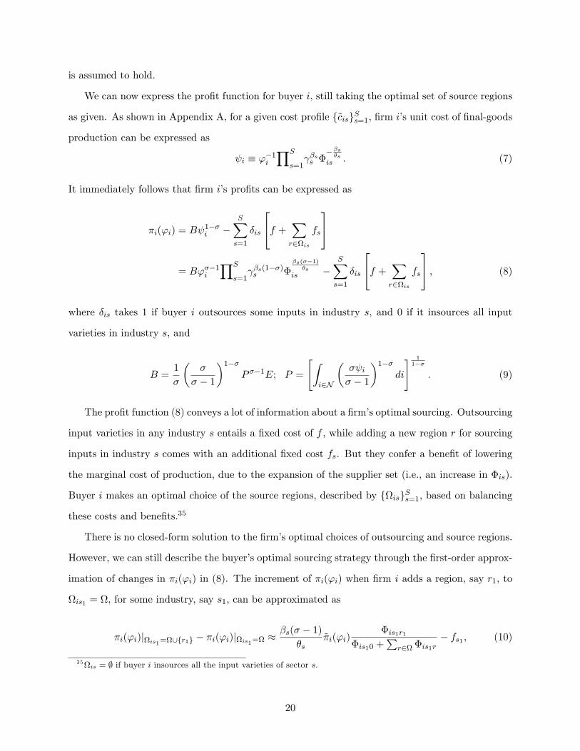
We can now express the profit function for buyer i, still taking the optimal set of source regions
as given. As shown in Appendix A, for a given cost profile cisSs=1, firm i’s unit cost of final-goods
production can be expressed as
ψi ≡ ϕ−1i
∏S
s=1γβss Φ
−βsθs
is . (7)
It immediately follows that firm i’s profits can be expressed as
πi(ϕi) = Bψ1−σi −
S∑s=1
δis
f +∑r∈Ωis
fs
= Bϕσ−1
i
∏S
s=1γβs(1−σ)s Φ
βs(σ−1)θs
is −S∑s=1
δis
f +∑r∈Ωis
fs
, (8)
where δis takes 1 if buyer i outsources some inputs in industry s, and 0 if it insources all input
varieties in industry s, and
B =1
σ
(σ
σ − 1
)1−σP σ−1E; P =
[∫i∈N
(σψiσ − 1
)1−σdi
] 11−σ
. (9)
The profit function (8) conveys a lot of information about a firm’s optimal sourcing. Outsourcing
input varieties in any industry s entails a fixed cost of f , while adding a new region r for sourcing
inputs in industry s comes with an additional fixed cost fs. But they confer a benefit of lowering
the marginal cost of production, due to the expansion of the supplier set (i.e., an increase in Φis).
Buyer i makes an optimal choice of the source regions, described by ΩisSs=1, based on balancing
these costs and benefits.35
There is no closed-form solution to the firm’s optimal choices of outsourcing and source regions.
However, we can still describe the buyer’s optimal sourcing strategy through the first-order approx-
imation of changes in πi(ϕi) in (8). The increment of πi(ϕi) when firm i adds a region, say r1, to
Ωis1 = Ω, for some industry, say s1, can be approximated as
πi(ϕi)|Ωis1=Ω∪r1 − πi(ϕi)|Ωis1=Ω ≈βs(σ − 1)
θsπi(ϕi)
Φis1r1
Φis10 +∑
r∈Ω Φis1r− fs1 , (10)
35Ωis = ∅ if buyer i insources all the input varieties of sector s.
20
where πi(ϕi) ≡ Bϕσ−1i
∏S
s=1γβs(1−σ)s Φ
βs(σ−1)θs
is denotes firm i’s operating profits. Whereas the incre-
ment of πi(ϕi) when it outsources inputs of industry s1 at all can be approximated as
πi(ϕi)|Ωis1=Ω − πi(ϕi)|Ωis1=∅ ≈βs(σ − 1)
θsπi(ϕi)
∑r∈Ω Φis1r
Φis10−(f +
∑r∈Ω
fs1
), (11)
where Ω 6= ∅. A region is more likely to be added if Φisr is greater, which is in turn the case if (i)
ns is larger, (ii) Tsr is larger, (iii) wr is smaller, or (iv) dir is smaller.
In equilibrium, inputs of industry s are outsourced if and only if (11) is nonnegative. In
principle, buyer i chooses its source regions for each outsourced industry s by selecting the regions
in a descending order from the region with the largest Φisr to the region with the smallest one as
long as adding a region gives the buyer a net benefit. However, such monotonicity of adding source
regions may not always hold if βs(σ − 1) < θs, which AFT call the substitutes case. Appendix A
shows some further details of the industry equilibrium, including its existence and uniqueness.
4.4 Testable Predictions
4.4.1 Global Sourcing
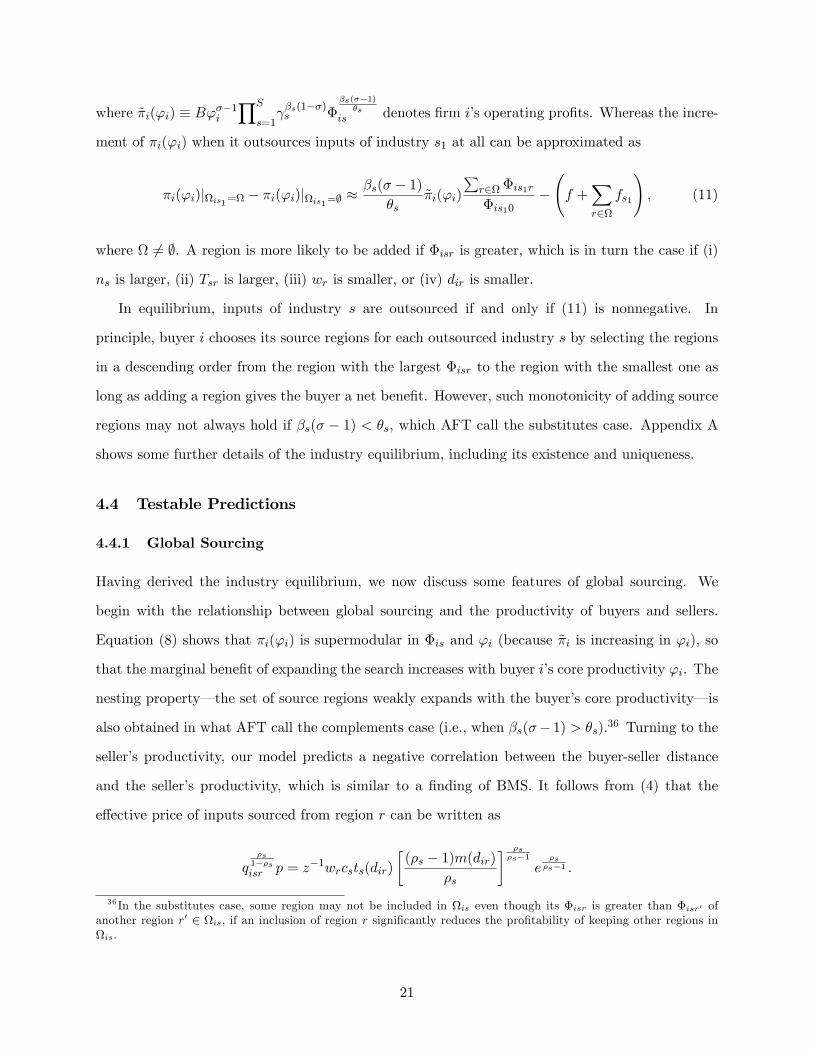
Having derived the industry equilibrium, we now discuss some features of global sourcing. We
begin with the relationship between global sourcing and the productivity of buyers and sellers.
Equation (8) shows that πi(ϕi) is supermodular in Φis and ϕi (because πi is increasing in ϕi), so
that the marginal benefit of expanding the search increases with buyer i’s core productivity ϕi. The
nesting property– the set of source regions weakly expands with the buyer’s core productivity– is
also obtained in what AFT call the complements case (i.e., when βs(σ− 1) > θs).36 Turning to the
seller’s productivity, our model predicts a negative correlation between the buyer-seller distance
and the seller’s productivity, which is similar to a finding of BMS. It follows from (4) that the
effective price of inputs sourced from region r can be written as
qρs
1−ρsisr p = z−1wrcsts(dir)
[(ρs − 1)m(dir)
ρs
] ρsρs−1
eρsρs−1 .
36 In the substitutes case, some region may not be included in Ωis even though its Φisr is greater than Φisr′ ofanother region r′ ∈ Ωis, if an inclusion of region r significantly reduces the profitability of keeping other regions inΩis.
21
The effective price of inputs sourced from a region increases with its distance from the buyer due to
the increasing trade costs, arising from a smaller chance of receiving high-quality inputs and greater
transport costs, while the distributions of the effective price of the inputs outsourced are common
across source regions as in Eaton and Kortum (2002). Consequently, inputs supplied from farther
regions tend to be produced by more effi cient firms than those in closer regions. Interpreting these
results from the viewpoint of domestic versus foreign sourcing, we show that buyers with higher
productivity tend to source from foreign suppliers and that foreign trade partners tend to be more
cost-effective than the domestic ones.
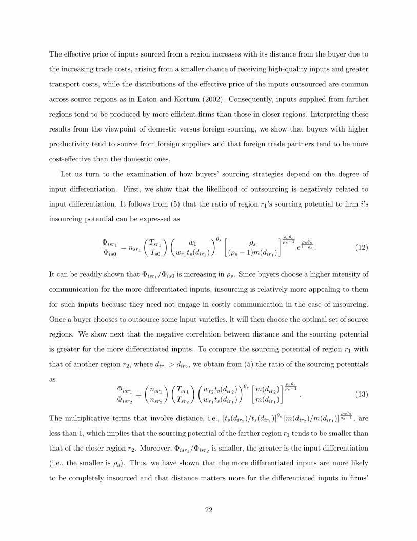
Let us turn to the examination of how buyers’ sourcing strategies depend on the degree of
input differentiation. First, we show that the likelihood of outsourcing is negatively related to
input differentiation. It follows from (5) that the ratio of region r1’s sourcing potential to firm i’s
insourcing potential can be expressed as
Φisr1
Φis0= nsr1
(Tsr1Ts0
)(w0
wr1ts(dir1)
)θs [ ρs(ρs − 1)m(dir1)
] ρsθsρs−1
eρsθs1−ρs . (12)
It can be readily shown that Φisr1/Φis0 is increasing in ρs. Since buyers choose a higher intensity of
communication for the more differentiated inputs, insourcing is relatively more appealing to them
for such inputs because they need not engage in costly communication in the case of insourcing.
Once a buyer chooses to outsource some input varieties, it will then choose the optimal set of source
regions. We show next that the negative correlation between distance and the sourcing potential
is greater for the more differentiated inputs. To compare the sourcing potential of region r1 with
that of another region r2, where dir1 > dir2 , we obtain from (5) the ratio of the sourcing potentials
asΦisr1
Φisr2
=
(nsr1nsr2
)(Tsr1Tsr2
)(wr2ts(dir2)
wr1ts(dir1)
)θs [m(dir2)
m(dir1)
] ρsθsρs−1
. (13)
The multiplicative terms that involve distance, i.e., [ts(dir2)/ts(dir1)]θs [m(dir2)/m(dir1)]ρsθsρs−1 , are
less than 1, which implies that the sourcing potential of the farther region r1 tends to be smaller than
that of the closer region r2. Moreover, Φisr1/Φisr2 is smaller, the greater is the input differentiation
(i.e., the smaller is ρs). Thus, we have shown that the more differentiated inputs are more likely
to be completely insourced and that distance matters more for the differentiated inputs in firms’
22
outsourcing decisions.
Proposition 1 The share of input varieties insourced and the share of input varieties sourced from
closer regions are both greater for the more differentiated inputs.
4.4.2 Reduction in Foreign Input Costs and Restructuring of Production Networks
We now examine how a reduction in foreign input costs affects firms’offshoring decisions and their
domestic sourcing strategies. We consider any changes that increase Φisr∗ for some foreign region
r∗ ∈ M + 1, · · · ,M +M∗, including a fall in wr∗ and an increase in Tsr∗ .
An increase in Φisr∗ makes region r∗ more attractive than before for all buyers. Consider the
case in which an increase in Φisr∗ induces some buyers to start sourcing inputs from region r∗.
Their individual sourcing capabilities, Φis, increase as a result, leading to lower marginal costs
of production. The buyers that have been outsourcing some inputs from region r∗ even before a
reduction in foreign input costs also enjoy lower marginal costs, while those that do not source any
inputs from region r∗ experience no change in their marginal costs.
As the costs of offshoring from region r∗ decrease, the marginal costs of production for both
continuous importers and import starters from region r∗ fall. Consequently, the price index P
falls and so does the demand shifter B in (9). Due to this increased intensity of product market
competition, not all the firms that import some inputs from region r∗ benefit from the reduction
in foreign input costs. As shown in (8) and (9), their operating profits increase if and only if the
increase in Φis is large enough that P σ−1ΠSs=1Φ
βs(σ−1)θs
is rises despite a fall in P .
Import starters restructure their production networks. In particular, offshoring directly induces
them to replace some domestic sellers (including themselves as input producers) with foreign sellers
(an effect that we refer to as the direct displacement effect). From Proposition 1, we learn that
these newly added foreign sellers tend to produce the less differentiated inputs. Thus, the displaced
domestic sellers tend to be from the less differentiated industries. In addition, import starters and
continuous importers may restructure their production networks as a consequence of the reduction
in their marginal costs (an effect that we refer to as the productivity effect). Their operating
profits unambiguously increase relative to those of non-importers, since a reduction in P affects all
final-good producers equally.
23
The productivity effect in turn affects a firm’s domestic production networks through two chan-
nels. First, it follows from (10) that import starters have a greater incentive to expand search
regions, relative to non-importers. Offshoring entails a rise in Φis so that each region r’s share
of input varieties, given by Φisr/Φis, drops. Consequently, for each input industry, some import
starters restructure their domestic supplier networks by adding distantly-located and productive
sellers, while dropping the less productive ones in all other source regions (an effect that we refer
to as the within-industry restructuring effect).37 Second, it follows from (11) that import starters
also have a greater incentive to begin outsourcing inputs in a new industry, particularly the dif-
ferentiated one that was not being sourced previously due to high variable trade costs (an effect
that we refer to as the industry composition effect). The following proposition summarizes the
testable predictions about the various effects of a fall in foreign input costs on the structure of
newly offshoring firms’domestic production networks.
Proposition 2 1. Relative to non-importers, import starters drop in every source region sellers
that are on average less productive than others in the same industries. This extent of dropping
is more profound in the newly-offshored industries, since the direct displacement effect that
some domestic suppliers are displaced by foreign suppliers is always present. Since the newly
offshored industries tend to be less differentiated, the dropped sellers in those industries tend
to be located farther and more productive than those in other industries.
2. Relative to non-importers, import starters add sellers that are on average more productive
and located farther than other firms within each previously-outsourced industry. In addition,
some import starters add sellers in industries from which they previously did not outsource
inputs. Since such newly-outsourced industries tend to be more differentiated and thus entail
higher communication costs, the sellers added in the newly-outsourced industries tend to be
located closer than those in the previously-outsourced industries.
Offshoring leads to the restructuring of firms’domestic production networks, thereby affecting
industry coagglomeration. The direct displacement effect induces coagglomeration as the sellers
that are directly replaced by foreign sellers tend to be located farther as they produce inputs that are
37We assume in this section that the distribution of ϕii∈N has a support that is wide enough to induce someimport starters to restructure their domestic supplier networks as their marginal costs of production decrease.
24

less differentiated than sellers in other industries. The two types of productivity effects of offshoring
on industry coagglomeration are mixed. On the one hand, the within-industry restructuring effect
implies that import starters replace the less productive sellers with the more productive ones,
which are located farther than others within the same industries. On the other hand, the industry
composition effect induces them to begin outsourcing inputs in the relatively more differentiated
industries so that they add sellers located closer than those in other industries. The following
proposition summarizes these possibilities.
Proposition 3 Although the effects of offshoring on industry coagglomeration are mixed, offshoring
induces industry coagglomeration if the within-industry restructuring effect is small relative to the
direct displacement and industry composition effects.
The proof of Proposition 3 is relegated to Appendix A. The basic idea is that if the fixed sourcing
costs are large so that within-industry restructuring in the newly offshored industries is limited, the
direct replacement and industry composition effects tend to dominate. Whether offshoring leads to
industry coagglomeration depends on the relative strength of the three effects of offshoring, which
we examine empirically in Section 5.3.
5 Regression Analyses and Results
In this section, we empirically examine using the network data the three testable hypotheses derived
in Section 4. For notational clarity, let us denote buyer, seller, industry (3-digit), and region (one of
47 prefectures) by i, j, s, and r, respectively. When industry and region fixed effects are included
in the regressions, we will be clear about whether they are for the buyer or seller.
5.1 Domestic Sourcing Patterns
We first examine Proposition 1, which is about the patterns of firms’domestic sourcing. Equation
(13) shows that firm i’s spatial pattern of domestic sourcing in industry s can be described by
Φisr1/Φisr2 , the ratio of the mass of input varieties procured from region r1 to that from region r2.
Let us denote firm i’s reference region of sourcing in industry s by rs(i), and use it to define the
denominator, Φisrs(i). It can be buyer i’s home region or the nearest region from which it sources
25
input s. We study the determinants of buyer i’s sourcing patterns according to the log of (13):
logΦisr
Φisrs(i)= − log nsrs(i) − log Tsrs(i) + θs logwrs(i) +
ρsθsρs − 1
logm(dirs(i))︸ ︷︷ ︸input-industry reference-region specific
(14)
+ log nsr + log Tsr − θs logwr︸ ︷︷ ︸input-industry source-region specific
− θsρs
ρs − 1× logm(dir)− θs log ts(dir)
We measure Φisr/Φisrs(i) by Nisr/Nisrs(i), the ratio of the number of industry-s sellers in region
r from which buyer i purchases inputs, relative to the counterpart in buyer i’s reference source
region. Notice that the first four terms are specific to the pair of an input industry and the buyer’s
reference source region, while the next three terms are specific to the pair of an input industry and
a source region. Instead of estimating each individual component (e.g. Tsr) on the right hand side
of (14), we include input-industry reference-region and input-industry source-region fixed effects to
absorb all seven terms in the regressions. The main variable of interest is θsρsρs−1 logm(dir), while
θs log ts(dir) will be controlled for by an interaction term that proxies for the input-industry specific
variable trade cost that increases in distance.
To quantify the effect of communication costs versus standard trade frictions, we parameterize
m(dir) and ts(dir) as:
m(dir) = dβir
ts(dir) = dγφsir
where φs captures the time sensitivity of the delivery of inputs (which gives the cross-industry
variation of transport costs).
With these parameterizations, we can express the empirical counterpart of (14) as
logNisr
Nisrs(i)= −β
[ρsθsρs − 1
log dir
]− γ [φsθs log dir] +
[FEsrs(i) + FEsr
]+ εirs, (15)
26
where an industry is defined as a JSIC 3-digit category.38 FEsrs(i) and FEsr stand for input-
industry reference-region and input-industry source-region fixed effects, respectively.39 With these
fixed effects included, we study the relationship between a buyer’s scope of domestic sourcing in a
region and the proximity of the source region (relative to the reference region from which it sources
the same type of inputs).40
To estimate β and γ, we need estimates of the model’s key parameters: ρs, θs and φs. We
measure ρs by the estimated elasticity of substitution between imported varieties in each industry s
in the U.S. from Soderbery (2015), who has improved the original estimates by Broda and Weinstein
(2006). The original estimates are at the HS 6-digit level, we use two concordance files and average
the estimates up to the JSIC 3-digit level, using sales weights obtained from Japan’s Census of
Manufacturers (see the Appendix for details). Since the focus of the paper is firms’sourcing of
intermediate inputs, when constructing ρs/ (ρs − 1), we exclude capital and consumption goods
according to the United Nations Broad Economic Categories (BEC) list.
We use two sets of estimates of θs. The first set is from Caliendo and Parro (2015), who estimate
θs using data on bilateral trade between 16 economies for 20 ISIC sectors. The second set of θs
is obtained from our own estimation using firm revenue data. In Section B.3 in the appendix, we
show how one can use the empirical distribution of firms’revenue to estimate θs. We show that
if a firm’s core productivity is distributed Fréchet with parameters T and θ, its revenue is also
distributed Fréchet, with the location parameter equal to TAθρ−1 and the shape parameter equal to
θ/(ρ− 1), where A is a sector-specific variable. Therefore, we can use the mean and the standard
deviation of firm revenue in the TSR data to back out θs (at the 3-digit JSIC level), given ρs. For
φs, we use the share of air freight costs in U.S. imports in industry s to proxy for the importance
of timely delivery (see the Appendix for details). The idea is that if the delivery of a good is time
sensitive, the slope of the variable trade cost with respect to distance is steeper.
Table 4 reports the estimates of β and γ, according to (15). Standard errors are clustered at
the input-industry-source-region level. In columns 1 to 6, we use a buyer’s nearest source region for
38We aggregate information from JSIC 4-digit to 3-digit because at the 4-digit level, a firm is unlikely to procureinputs from multiplier prefectures. All our empirical results remain largely robust to including 4-digit input industryand buyer industry fixed effects. The results are available upon request.39These fixed effects can capture any unobserved characteristics of a buyer’s location and industry (e.g., the effects
of infrastructure and agglomeration), as well as a seller’s location and industry.40We use the capital city of a prefecture to compute the distance.
27
each industry as the reference region, while in columns 7 through 9, we use a buyer’s home region
as the reference point. The cost of using a buyer’s home region as the reference point is that not all
buyers procure inputs in each sector from its home region. Thus, the number of observations will
be smaller in the last three columns. When using the estimated θs from Caliendo and Parro (2014),
we find in columns 1 to 3 that a buyer’s scope of domestic sourcing is decreasing in distance, more
so for differentiated inputs. Specifically, as reported in column 1, a 10% increase in the distance
relative to the nearest region is associated with a 0.5% drop in the number of sellers for an industry
that has the mean value of θs (=9.82).41 Column 2 shows that such negative correlation is more
pronounced for the more differentiated inputs, as proxied by ρs/ (ρs − 1). Sectors that have a one
standard-deviation larger ρs/ (ρs − 1) (=0.26), compared to the mean value of 1.33, is associated
with an additional 0.15% drop in the number of sellers from a region that is 10% farther away
compared to the reference region, evaluated at the same mean value of θs.42 Column 3 shows that
the results remain robust after we control for the interaction between log dir and the share of air
freight cost in imports of the corresponding U.S. industry, φs (Hummels and Schaur, 2013).
In columns 4 to 6, when we use the firm-based estimate of θs, we find quantitatively larger effects.
According to the coeffi cient on ρsθsρs−1 log (dir) in column 6, sectors that have one standard-deviation
larger ρs/ (ρs − 1) compared to the sectoral mean are associated with an additional 0.19% drop in
the number of sellers from a region that is 10% away in distance relative to the reference region,
evaluated at the mean value of θs (=13.72).43 The results become quantitatively more significant
when we use the buyer’s home region as the reference region (see columns 7 to 9), or when we use the
2010 sample (see Table A5 in the appendix), or when we include the parent-children relationships
(results available upon request).
In Table 5, we empirically examine the pattern of firms’domestic sourcing at the extensive
margin, by replacing the dependent variable in specification (15) with a dummy for whether buyer
i sources intermediates in industry s from source region r or not. Since we only have information
on firms’foreign sourcing at the broad sector level (12 manufacturing sectors) from BSJBSA, we
consider a firm’s participation in domestic and foreign sourcing respectively at the broad sector level.
Information on firms’ domestic sourcing at the more disaggregated industry level is aggregated
41−0.47% = −0.00535× 10× 9.82%42−0.145% = −0.00565× 10× 9.82× 0.262%43−0.188% = −0.00524× 10× 13.717× 0.262%
28
to the broad sector level.44 Accordingly, we compute the weighted average of input industries’
characteristics across 3-digit industries within a broad sector. The procedures of aggregation are
described in detail in the data appendix. Since we no longer use information of the reference source
region to define the dependent variable, we drop FEsrs(i) as a regressor, while retaining input-
industry source-region (FEsr) fixed effects. We sometimes include buyer fixed effects as well to
control for any unobservable determinants of domestic sourcing (e.g., buyer’s productivity).
We use the estimated θs from Caliendo and Parro (2014) in Panel A, and our own estimates
using firm-level data in Panel B. Regardless of the estimates, we find that a buyer’s likelihood of
sourcing inputs from a prefecture is decreasing in the bilateral distance (columns 1 and 7), after
controlling for input-industry source-region fixed effects. The negative correlation is stronger for
the more differentiated inputs (columns 2-3 and columns 8-9, respectively). These regression results
remain robust and quantitatively similar after we control for buyer fixed effects (columns 4-6 and
columns 10-12, respectively). We find that the differential effect of distance on the incidence of
domestic sourcing across industries is economically significant. Based on the coeffi cients reported in
column 4, a 10% increase in distance relative to the home region is associated with a 0.1 percentage-
point decline in the likelihood of sourcing from the region, evaluated at the mean value of θs.45
Based on the estimates in column 5 and the mean value of θs, the same distance is associated with
an additional 0.1 percentage-point decline in the likelihood of sourcing for industries with a one
standard-deviation larger ρs/ (ρs − 1) relative to the sectoral mean.46
In Table 6, we study the determinants of a firm’s decision to offshore inputs in an industry.
Without detailed information about the source country of offshoring, we examine Proposition 1
on offshoring by including a buyer’s (log) TFP and the interaction term between (log) TFP and
ρs/ (ρs − 1). Our model predicts that more productive firms are more likely to incur the fixed costs
to offshore intermediates. Given that trade costs will be increasing in input industry’s product
differentiation, such positive relationship should be weaker for the more differentiated inputs. Re-
44For instance, the dummy for a firm’s domestic sourcing is set equal to 1 for a broad sector if the firm outsourcesin any 3-digit industry that belongs to the sector.45Using the coeffi cient on ln(dist+1)×θs (=−0.001) and the mean value of θs (=9.82) we come up with −0.098% =−0.001× 10× 9.82%.46Given that the mean and the standard deviation of ρs/ (ρs − 1) are 1.328 and 0.262 (across 3-digit industries,
see Table A9 in the appendix), respectively, the increase in the likelihood of sourcing from a region is −0.004 ×0.262︸ ︷︷ ︸
std of ρs/(ρs−1)
× 10× 9.82︸︷︷︸θs
%.
29

gardless of which estimated θs used, we find a positive and significant correlation between a buyer’s
likelihood of offshoring inputs and its productivity, after controlling for input-industry source-region
fixed effects. Such correlation is weaker for the more differentiated input industries (see columns 1
and 3). These results remain robust even after we control for buyer fixed effects in columns 2 and
4. We also find that a buyer’s domestic sourcing in an input industry is positively related to the
likelihood of offshoring in the same industry. This result implies that fixed costs to offshore could
be lower if a firm already incurs some of them for domestic sourcing. This pattern of sequential
sourcing will be the basis for the construction of our instrument.
5.2 Relationship between Firms’Global Sourcing and Domestic Supplier Choices
The final part of the paper studies Propositions 2 and 3, which are about the effect of firms’
offshoring on their choices of domestic suppliers. We first examine whether the likelihood of a
buyer’s dropping and adding domestic suppliers is associated with an exogenously induced offshoring
decision. To this end, we estimate the following specification using our two-year panel data on
Japan’s production networks (2005 and 2010):
Iij = β∆impi+γ∆impi×log
(xijxi
)+δ log salesi+
[FEs(i) + FEr(i) + FEs(j) + FEr(j)
]+εij , (16)
where Iij is a dummy variable indicating whether buyer i drops (or adds) seller j between 2005 and
2010. Each unit of observation is a buyer-seller link. The regression sample excludes all existing
importers in 2005, as our goal is to study the effect of the participation in offshoring, rather than
that of the extent of offshoring.
When we run the “drop”regressions, we further restrict the sample by excluding each buyer’s
newly added seller links, such that we can gauge the effect of offshoring on a firm’s decisions of
dropping an existing domestic seller. In particular, the dependent variable of the “drop”regressions
is defined as Iij = Dropij , which is equal to 1 if seller j and buyer i were linked in 2005 but not
anymore in 2010, and 0 otherwise (if the relationship continued).
When we run the “add”regressions, on the other hand, we restrict the sample by excluding each
buyer’s dropped seller links, such that we can empirically compare the characteristics between the
buyer’s continuing suppliers with those of its newly added suppliers, after it offshores inputs. The
30
dependent variable of the “add”regressions is defined as Iij = Addij , which is equal to 1 if a new
link between buyer i and seller j is observed in the 2010 sample but not in 2005, and 0 otherwise
(indicating an old relationship).47
The variable ∆impi is a dummy indicating firm i’s switching from no offshoring in 2005 to
offshoring any inputs between 2005 and 2010.48 The regressor of interest is the interaction term
∆impi × log(xijxi
), where xij
xirepresents a measure of a supplier’s characteristic, relative to the
average characteristics of the sellers used by buyer i in 2005. We use a demeaned measure since a
buyer compares the candidate supplier with its existing suppliers when making decisions to add or
drop suppliers. For instance, a supplier considered to be large by a firm may not be considered large
by another firm. More specifically, in the “drop”regressions, xi is constructed using the sample of
sellers from which the buyer procured inputs in 2005. On the other hand, in the “add”regressions,
xi is constructed using sellers from which the buyer procured inputs in 2010 (i.e., those that were
dropped since 2005 will not be included in the construction of the buyer’s mean). We consider two
seller characteristics– log size (measured by either sales or employment) and log distance from a
buyer. Buyer-industry (FEs(j)), buyer-region (FEr(i)), input-industry (FEs(j)), and source-region
(FEr(j)) fixed effects are always included to control for any region- and industry-specific trends of
supplier adding and dropping, such as external economies of scale for different industries, initial
levels of economic development, or local government policies.49
To establish causality, we estimate specification (16) via two-stage least squares (2SLS). We
construct an instrument at the buyer level. We first follow Hummels et al. (2014) to measure the
world export supply (WES) shocks in each industry s during our sample period as:
WESs = ln (exps,2010)− ln (exps,2005) , (17)
where exps,t is the global exports to all destination countries in the world except Japan.50
47Notice that the results for the “add” regressions should not be interpreted as the effects on the likelihood ofsourcing. The coeffi cient on the interaction term shows the difference in the average seller’s characteristics betweennew and continuing relationships.48Recall that we do not have information on firms’imports by sector.49When we control for buyer fixed effects, the coeffi cients on the interactions have the same sign and remain
significant. The drawback is that we will no longer be able to identify the independent effect of ∆impi on buyers’supplier adding and dropping.50The regression results are robust to alternative measures of WES using only data from exporting countries that
were Japan’s top trade partners in 2005 or those from destination countries that are either OECD or advancedeconomies.
31
To construct the instruments for offshoring at the firm level, we exploit the information about
a firm’s sectoral pattern of domestic sourcing. In Table 5, we find that firms are more likely to
offshore inputs in an industry in which it has already sourced inputs domestically. These results
are suggestive of a lower fixed cost of offshoring, conditional on the firm’s domestic sourcing in
the same industry. Thus, foreign countries’export supply shocks in an industry are more likely to
induce a Japanese firm to start offshoring if it has already sourced inputs in the same industry.
Based on these findings, we merge a firm’s sectoral pattern of domestic outsourcing with that of
the vector of estimated export supply shocks, and compute firm i’s exposure to the world export
supply shocks as
shocki =
S∑s=1
φisWESs, (18)
where φis is a dummy, which equals 1 if buyer i outsources industry-s inputs domestically in 2005,
and 0 otherwise. We construct such dummies at the Japanese 4-digit SIC level (i.e., S = 563
manufacturing industries).
We use shocki specified in (18) as an instrument for∆impi, and shocki×logxijxias an instrument
for ∆impi × logxijxi, as suggested by Wooldridge (2010). Table 7 reports both the OLS and 2SLS
results of estimating (16) for dropping, based on the sample of all buyers in the manufacturing sector
that sourced inputs domestically but not from foreign suppliers in 2005. As reported in columns 1
to 4, while the OLS estimated coeffi cient on ∆impi and ∆impi × logxijxitake the expected signs,
they are all insignificant.51 The 2SLS estimates in columns 5 to 8, however, show statistically
significant effects of offshoring on firms’dropping of domestic suppliers. In column 5, the estimated
coeffi cient on ∆impi shows that a buyer’s offshoring decision reduces the likelihood of dropping
domestic suppliers. Within buyer industries, buyer home regions, input industries, and source
regions, a buyer that started importing since 2005 is on average 65% less likely to drop its existing
sellers between 2005 and 2010. In column 6, we find that even though newly offshoring firms tend
to be less likely to drop domestic suppliers, they are relatively more likely to drop the larger one
(columns 7 and 8). In particular, the coeffi cient of 0.087 on the interaction term in column 7 implies
that an existing supplier that is 50% larger than the mean supplier of a buyer is 4.3% relatively
51The main endogeneity that we aim to tackle is a firm’s positive supply shock that may trigger its offshoring on theone hand, but affect the probability of dropping domestic suppliers in either direction on the other. The insignificantresults based via OLS do not contradict our significant 2SLS results.
32
more likely to be dropped on average. If we measure firm size by employment, the differential effect
would be 6.5% according to the coeffi cient of 0.129 on the interaction term reported in column 8.
All F statistics for the first stages of these 2SLS estimations suggest that our instruments pass the
weak instrument test by a wide margin. Table A6 in the Appendix reports the regression results
of the first stage. The coeffi cients on the instrument and its interaction with seller characteristics
are statistically significant when the corresponding endogenous variables are used as the dependent
variables of the first stage.
Table 8 reports the estimates of the “add”regressions based on specification (16). Columns 1
to 4 report the OLS estimates. It is not surprising that there is a positive correlation between a
firm’s import dummy and likelihood of having a new domestic supplier. For instance, a positive
productivity shock will induce a firm to add both domestic and foreign suppliers simultaneously.
As reported in columns 5 to 8, the 2SLS estimates show that the newly offshoring firms are less
likely to add the relatively more distant domestic suppliers (column 6), but more likely to add the
larger ones (columns 7 and 8).
The findings that newly offshoring firms are more likely to add larger suppliers seem to contradict
the earlier findings that they are also more likely to drop larger suppliers, as reported in Table 7.
However, through the lens of our model, these results can be rationalized by the joint force of the
direct displacement, within-industry restructuring and industry composition effects of offshoring.
The findings that larger domestic suppliers are more likely to be dropped are consistent with the
direct displacement effect. Offshoring firms’ substitute domestic generic-input suppliers, which
tend to be larger and more distantly located, with foreign suppliers producing similar inputs. The
results that larger domestic suppliers are more likely to be added can be due to the within-industry
restructuring effect of offshoring that induces firms to add more productive and distant domestic
suppliers within each industry. The fact that more distant suppliers are less likely to be added can
be explained by the industry composition effect– differentiated input industries, from which a buyer
previously did not source inputs, are now being added to the buyer’s sourcing set. Considering
the rise in communication costs, the buyer will source inputs from closer domestic suppliers in
the newly added, differentiated industries. Table A7 in the Appendix shows that the coeffi cients
on the instrument and its interaction with seller characteristics are statistically significant in the
corresponding first-stage regressions.
33
To further study the three effects of offshoring, in particular the industry composition effect,
we empirically examine the relationship between firms’offshoring and the pattern of adding and
dropping of input industries. To this end, we estimate the following specification:
Iis = βs∆impi + γs∆impi ×Xs +[FEs(i) + FEr(i) + FEs(j)
]+ ξis, (19)
where Iis is a dummy variable indicating whether buyer i drops (or adds) industry s between 2005
and 2010. Each unit of observation is a buyer-input-industry pair. Similar to the sample we used
to estimate (16), the regression sample excludes all buyers that already imported inputs in 2005.
When we run the “drop”regressions, we further restrict the sample by excluding each buyer’s
newly added input industries, such that we can gauge the effect of offshoring on a firm’s decisions
of dropping an existing input industry. The dependent variable is defined as Iis = Dropis, which is
equal to 1 if buyer i sourced inputs in industry s in 2005 but stopped sourcing in the same industry
in 2010, and 0 otherwise.
When we run the “add”regressions, we restrict the sample by excluding each buyer’s dropped
input industries since 2005, such that we can gauge the effect of offshoring on a firm’s decisions to
add new industries, based on their industry characteristics compared to continuing input industries.
To consider a full matrix of industries that a buyer can consider adding, we create a regression
sample by setting Iis = Addis = 0 for all input industries from which buyer i did not source inputs
in both 2005 and 2010, but equal to 1 for those from which buyer i did not source inputs in 2005
but started sourcing inputs in or before 2010.
The variable of interest, ∆impi × Xs, is an interaction term between the change in buyer i’s
import status and industry s’s product differentiation (Xs), measured by either ρs/ (ρs − 1) or the
Rauch indicator, which equals 1 for differentiated goods, and 0 otherwise (see Section B.1 in the
Appendix for details). Buyer industry (FEs(i)), home region (FEr(i)), and input industry fixed
effects (FEs(j)) are always included.
Table 9 presents the estimates of (19) via OLS and 2SLS. By using shocki as an instrument for
∆impi, and shocki×Xs as an instrument for∆impi×Xs, we find in our 2SLS regressions that newly
offshoring firms are less likely to drop (as measured by the Rauch indicator in column 5) but more
likely to add the more differentiated industries for domestic sourcing (both columns 7 and 8). These
34
patterns of input industry adding and dropping support the model predictions, and are consistent
with the hypothesis that the industry composition effect and the direct displacement effect are the
main reasons for why closer suppliers are more likely to be added, while larger suppliers are more
likely to be dropped, after a firm offshores inputs. Table A8 in the Appendix reports the regression
results of the first stage.
6 Concluding Remarks
In this paper, we study from both theoretical and empirical perspectives the spatial and sectoral
patterns of firms’global sourcing, as well as the effect of offshoring on firms’domestic production
networks. We develop a multi-region global sourcing model in which firms source inputs from
suppliers in various input industries that differ in the degree of product differentiation. Firms choose
the optimal level of communication with suppliers, depending on the inputs’product differentiation.
Using exhaustive data on buyer-seller links in Japan, we find that the more productive firms
source inputs from more suppliers and domestic regions, including the more distant ones. Distant
suppliers are more productive on average, while productive firms are more likely to offshore in-
puts. The negative correlation between distance and the extent of domestic sourcing is stronger
for differentiated inputs. Using a firm-level instrument based on the sectoral patterns of buyers’
initial domestic sourcing and global export supply shocks, we study the causal impact of a firm’s
offshoring on its choices of domestic suppliers. We find that upon offshoring, firms are less likely to
drop domestic suppliers on average, but are relatively more likely to drop the larger ones. Newly
offshoring firms tend to add domestic suppliers that are relatively larger but also those that are
more proximate. These findings suggest that the within-industry restructuring and industry com-
position effects of offshoring, both arising from declines in marginal costs, play important roles in
shaping firms’domestic production networks. The resulting reorganization of firms’domestic sup-
plier relationships reduces the average distance between buyers and sellers, increasing the spatial
concentration of production clusters in Japan.
Lower communication and transportation costs obviously have made production more global.
Our paper shows that while input sourcing has become more spatially dispersed across countries,
it may lead to localization of production within a nation or region. These results echo the World
35

Trade Organization’s (2013) findings about the increasingly regionalized global value chains. We
leave the analysis about the macroeconomic implications of the increasing localization of production
networks for future research.
Hitotsubashi University
Gakushuin University
Senshu University
Johns Hopkins University and CESIfo
36

A Appendix for the Theory
A.1 Firm’s Cost Minimization Problem
Given a distribution function of the prices for the input varieties for every sector s, which is
denoted by Gisr(p), firm i chooses the input levels xisr(p)p∈[0,∞) to minimize the cost of producing
composite input s. The unit cost function for firm i is the solution to the minimization problem:
minxisr(·)r∈0∪Ωis
∑r∈0∪Ωis
µ(Iisr)
∫ ∞0
pxisr(p)dGisr(p)
s.t
µ(Iis0)
∫ ∞0
xis0(p)ρs−1ρs dGis0(p) +
∑r∈Ωis
qisrµ(Iisr)
∫ ∞0
xisr(p)ρs−1ρs dGisr(p)
ρsρs−1
≥ 1.
By solving this problem, we obtain the optimal input levels as
xis0(p) = p−ρs
µ(Iis0)
∫ ∞0
p1−ρsdGis0(p) +∑r∈Ωis
µ(Iisr)
∫ ∞0
(q
ρs1−ρsisr p
)1−ρsdGis0(p)
ρs
1−ρs
,
xisr(p) = p−ρsqρsisr
µ(Iis0)
∫ ∞0
p1−ρsdGis0(p) +∑r′∈Ωis
µ(Iisr′)
∫ ∞0
(q
ρs1−ρsisr′ p
)1−ρsdGis0(p)
ρs
1−ρs
, for r ∈ Ωis.
Substituting these solutions to∑
r∈0∪Ωisµ(Iisr)
∫∞0 pxisr(p)dGisr(p) gives us the unit cost cis
given in (3).
A.2 Optimal Sourcing and the Unit Cost of Final Good Production for a Given
Sets of Source Regions
The unit cost of inputs equals p = z−1w0cs for insourced inputs, while it equals
qρs
1−ρsisr p = z−1q
ρs1−ρsisr wrcsts(dir)e
ms(dir)qisr
for inputs outsourced to sellers in region r. Following Eaton and Kortum (2002), we obtain the
distribution function of effective prices, p ≡ qρs
1−ρsisr p, for each source region r as
Gisr(p) = 1− e−Φisr pθs, for r ∈ 0 ∪ Ωis,
37
where Φisr is defined in (5).
The input-price (or input-cost) probability distribution for every input variety of type s is
common across source regions and can be written as
Gis(p) = 1− e−Φispθs, where Φis = Φis0 +
∑r∈Ωis
Φisr;
and hence the unit cost of the composite input s is given by cis = γsΦ− 1θs
is , where γs ≡ Γ(θs+1−ρs
θs
) 11−ρs .
For a given cost profile cisSs=1, the optimal level of the composite input s to produce each unit of
the final good equals xis = βsϕicis
ΠSj=1c
βjij . Consequently, the unit cost of a final good is given by
ψi ≡S∑s=1
cisxis =1
ϕiΠSs=1c
βsis =
1
ϕiΠSs=1γ
βss Φ
−βsθs
is .
A.3 Sourcing Strategy and Industry Equilibrium
As AFT points out, buyers’ choice of source regions requires some consideration as to whether
the choice of individual source regions exhibits substitutability. To see this, we examine how an
addition of a source region, say region r2, affects the sourcing potential of another source region,
say region r1, within the same input industry by taking a further difference of the expression in
(10):
[πi(ϕi)|Ωis∪r1,r2 − πi(ϕi)|Ωis∪r2]− [πi(ϕi)|Ωis∪r1 − πi(ϕi)|Ωis ]
≈ βs(σ − 1)
θs
[βs(σ − 1)
θs− 1
]πi(ϕi)
Φisr1
Φis0 +∑
r∈ΩisΦisr
Φisr2
Φis0 +∑
r∈ΩisΦisr
. (20)
We see immediately that the profit function is supermodular in Φisr1 and Φisr2 if βs(σ − 1) > θs,
which AFT call the complements case, while it is submodular if βs(σ− 1) < θs, which is called the
substitutes case. Adding a source region increases the sourcing potential of other regions in the
complements case, while it decreases the sourcing potential of other regions in the substitutes case.
In contrast, the first-order approximation of the impact of an inclusion of region r2 as a source
38
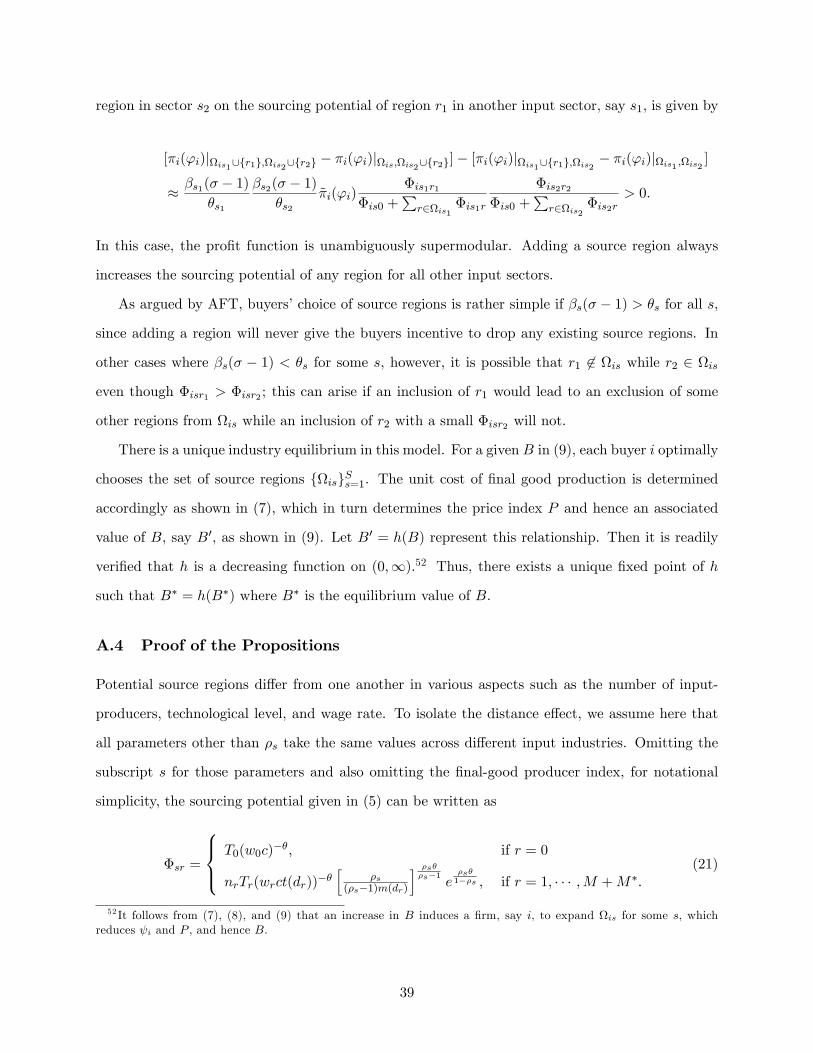
region in sector s2 on the sourcing potential of region r1 in another input sector, say s1, is given by
[πi(ϕi)|Ωis1∪r1,Ωis2∪r2 − πi(ϕi)|Ωis,Ωis2∪r2]− [πi(ϕi)|Ωis1∪r1,Ωis2 − πi(ϕi)|Ωis1 ,Ωis2 ]
≈ βs1(σ − 1)
θs1
βs2(σ − 1)
θs2πi(ϕi)
Φis1r1
Φis0 +∑
r∈Ωis1Φis1r
Φis2r2
Φis0 +∑
r∈Ωis2Φis2r
> 0.
In this case, the profit function is unambiguously supermodular. Adding a source region always
increases the sourcing potential of any region for all other input sectors.
As argued by AFT, buyers’choice of source regions is rather simple if βs(σ − 1) > θs for all s,
since adding a region will never give the buyers incentive to drop any existing source regions. In
other cases where βs(σ − 1) < θs for some s, however, it is possible that r1 6∈ Ωis while r2 ∈ Ωis
even though Φisr1 > Φisr2 ; this can arise if an inclusion of r1 would lead to an exclusion of some
other regions from Ωis while an inclusion of r2 with a small Φisr2 will not.
There is a unique industry equilibrium in this model. For a given B in (9), each buyer i optimally
chooses the set of source regions ΩisSs=1. The unit cost of final good production is determined
accordingly as shown in (7), which in turn determines the price index P and hence an associated
value of B, say B′, as shown in (9). Let B′ = h(B) represent this relationship. Then it is readily
verified that h is a decreasing function on (0,∞).52 Thus, there exists a unique fixed point of h
such that B∗ = h(B∗) where B∗ is the equilibrium value of B.
A.4 Proof of the Propositions
Potential source regions differ from one another in various aspects such as the number of input-
producers, technological level, and wage rate. To isolate the distance effect, we assume here that
all parameters other than ρs take the same values across different input industries. Omitting the
subscript s for those parameters and also omitting the final-good producer index, for notational
simplicity, the sourcing potential given in (5) can be written as
Φsr =
T0(w0c)
−θ, if r = 0
nrTr(wrct(dr))−θ[
ρs(ρs−1)m(dr)
] ρsθρs−1
eρsθ
1−ρs , if r = 1, · · · ,M +M∗.(21)
52 It follows from (7), (8), and (9) that an increase in B induces a firm, say i, to expand Ωis for some s, whichreduces ψi and P , and hence B.
39
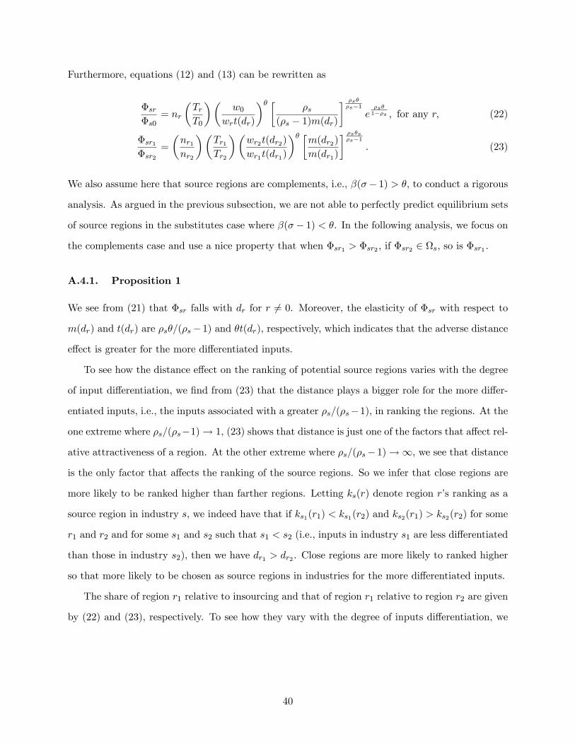
Furthermore, equations (12) and (13) can be rewritten as
Φsr
Φs0= nr
(TrT0
)(w0
wrt(dr)
)θ [ ρs(ρs − 1)m(dr)
] ρsθρs−1
eρsθ
1−ρs , for any r, (22)
Φsr1
Φsr2
=
(nr1nr2
)(Tr1Tr2
)(wr2t(dr2)
wr1t(dr1)
)θ [m(dr2)
m(dr1)
] ρsθsρs−1
. (23)
We also assume here that source regions are complements, i.e., β(σ− 1) > θ, to conduct a rigorous
analysis. As argued in the previous subsection, we are not able to perfectly predict equilibrium sets
of source regions in the substitutes case where β(σ− 1) < θ. In the following analysis, we focus on
the complements case and use a nice property that when Φsr1 > Φsr2 , if Φsr2 ∈ Ωs, so is Φsr1 .
A.4.1. Proposition 1
We see from (21) that Φsr falls with dr for r 6= 0. Moreover, the elasticity of Φsr with respect to
m(dr) and t(dr) are ρsθ/(ρs− 1) and θt(dr), respectively, which indicates that the adverse distance
effect is greater for the more differentiated inputs.
To see how the distance effect on the ranking of potential source regions varies with the degree
of input differentiation, we find from (23) that the distance plays a bigger role for the more differ-
entiated inputs, i.e., the inputs associated with a greater ρs/(ρs−1), in ranking the regions. At the
one extreme where ρs/(ρs−1)→ 1, (23) shows that distance is just one of the factors that affect rel-
ative attractiveness of a region. At the other extreme where ρs/(ρs− 1)→∞, we see that distance
is the only factor that affects the ranking of the source regions. So we infer that close regions are
more likely to be ranked higher than farther regions. Letting ks(r) denote region r’s ranking as a
source region in industry s, we indeed have that if ks1(r1) < ks1(r2) and ks2(r1) > ks2(r2) for some
r1 and r2 and for some s1 and s2 such that s1 < s2 (i.e., inputs in industry s1 are less differentiated
than those in industry s2), then we have dr1 > dr2 . Close regions are more likely to ranked higher
so that more likely to be chosen as source regions in industries for the more differentiated inputs.
The share of region r1 relative to insourcing and that of region r1 relative to region r2 are given
by (22) and (23), respectively. To see how they vary with the degree of inputs differentiation, we
40
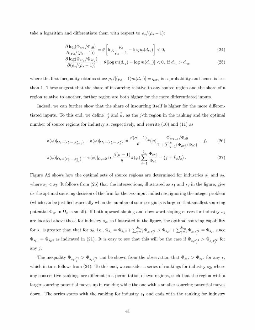
take a logarithm and differentiate them with respect to ρs/(ρs − 1):
∂ log(Φsr1/Φs0)
∂(ρs/(ρs − 1))= θ
[log
ρsρs − 1
− logm(dr1)
]< 0, (24)
∂ log(Φsr1/Φsr2)
∂(ρs/(ρs − 1))= θ [logm(dr2)− logm(dr1)] < 0, if dr1 > dr2 , (25)
where the first inequality obtains since ρs/[(ρs − 1)m(dr1)] = qsr1 is a probability and hence is less
than 1. These suggest that the share of insourcing relative to any source region and the share of a
region relative to another, farther region are both higher for the more differentiated inputs.
Indeed, we can further show that the share of insourcing itself is higher for the more differen-
tiated inputs. To this end, we define rsj and ks as the j-th region in the ranking and the optimal
number of source regions for industry s, respectively, and rewrite (10) and (11) as
π(ϕ)|Ωs=rs1,··· ,rsk+1 − π(ϕ)|Ωs=rs1,··· ,rsk ≈β(σ − 1)
θπ(ϕ)
Φsrk+1/Φs0
1 +∑k
j=1(Φsrsj/Φs0)
− fs, (26)
π(ϕ)|Ωs=rs1,··· ,rsks − π(ϕ)|Ωs=∅ ≈β(σ − 1)
θπ(ϕ)
ks∑j=1
Φsrsj
Φs0−(f + ksfs
). (27)
Figure A2 shows how the optimal sets of source regions are determined for industries s1 and s2,
where s1 < s2. It follows from (26) that the intersections, illustrated as s1 and s2 in the figure, give
us the optimal sourcing decision of the firm for the two input industries, ignoring the integer problem
(which can be justified especially when the number of source regions is large so that smallest sourcing
potential Φsr in Ωs is small). If both upward-sloping and downward-sloping curves for industry s1
are located above those for industry s2, as illustrated in the figure, the optimal sourcing capability
for s1 is greater than that for s2, i.e., Φs1 = Φs10 +∑ks1
j=1 Φs1rs1j> Φs20 +
∑ks2j=1 Φs2r
s1j
= Φs2 , since
Φs10 = Φs20 as indicated in (21). It is easy to see that this will be the case if Φs1rs1j> Φs2r
s2jfor
any j.
The inequality Φs1rs1j> Φs2r
s2jcan be shown from the observation that Φs1r > Φs2r for any r,
which in turn follows from (24). To this end, we consider a series of rankings for industry s2, where
any consecutive rankings are different in a permutation of two regions, such that the region with a
larger sourcing potential moves up in ranking while the one with a smaller sourcing potential moves
down. The series starts with the ranking for industry s1 and ends with the ranking for industry
41
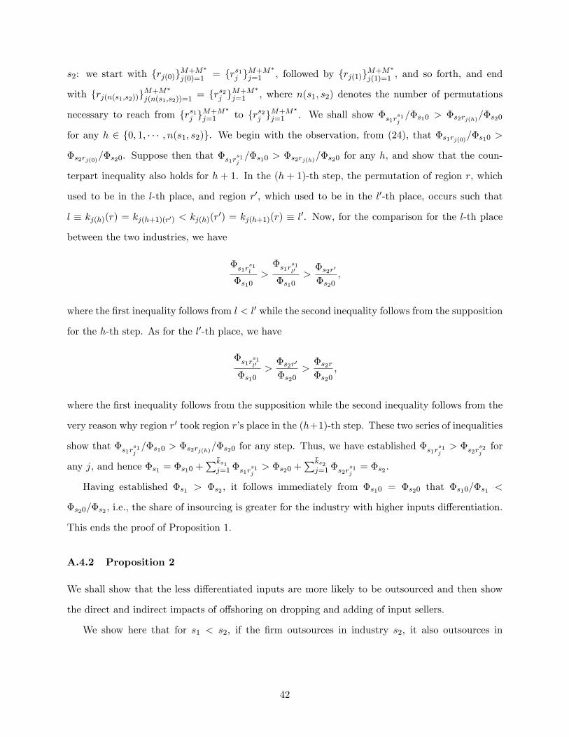
s2: we start with rj(0)M+M∗
j(0)=1 = rs1j M+M∗
j=1 , followed by rj(1)M+M∗
j(1)=1 , and so forth, and end
with rj(n(s1,s2))M+M∗
j(n(s1,s2))=1 = rs2j M+M∗
j=1 , where n(s1, s2) denotes the number of permutations
necessary to reach from rs1j M+M∗
j=1 to rs2j M+M∗
j=1 . We shall show Φs1rs1j/Φs10 > Φs2rj(h)
/Φs20
for any h ∈ 0, 1, · · · , n(s1, s2). We begin with the observation, from (24), that Φs1rj(0)/Φs10 >
Φs2rj(0)/Φs20. Suppose then that Φs1r
s1j/Φs10 > Φs2rj(h)
/Φs20 for any h, and show that the coun-
terpart inequality also holds for h + 1. In the (h + 1)-th step, the permutation of region r, which
used to be in the l-th place, and region r′, which used to be in the l′-th place, occurs such that
l ≡ kj(h)(r) = kj(h+1)(r′) < kj(h)(r′) = kj(h+1)(r) ≡ l′. Now, for the comparison for the l-th place
between the two industries, we have
Φs1rs1l
Φs10>
Φs1rs1l′
Φs10>
Φs2r′
Φs20,
where the first inequality follows from l < l′ while the second inequality follows from the supposition
for the h-th step. As for the l′-th place, we have
Φs1rs1l′
Φs10>
Φs2r′
Φs20>
Φs2r
Φs20,
where the first inequality follows from the supposition while the second inequality follows from the
very reason why region r′ took region r’s place in the (h+1)-th step. These two series of inequalities
show that Φs1rs1j/Φs10 > Φs2rj(h)
/Φs20 for any step. Thus, we have established Φs1rs1j> Φs2r
s2jfor
any j, and hence Φs1 = Φs10 +∑ks1
j=1 Φs1rs1j> Φs20 +
∑ks2j=1 Φs2r
s1j
= Φs2 .
Having established Φs1 > Φs2 , it follows immediately from Φs10 = Φs20 that Φs10/Φs1 <
Φs20/Φs2 , i.e., the share of insourcing is greater for the industry with higher inputs differentiation.
This ends the proof of Proposition 1.
A.4.2 Proposition 2
We shall show that the less differentiated inputs are more likely to be outsourced and then show
the direct and indirect impacts of offshoring on dropping and adding of input sellers.
We show here that for s1 < s2, if the firm outsources in industry s2, it also outsources in
42
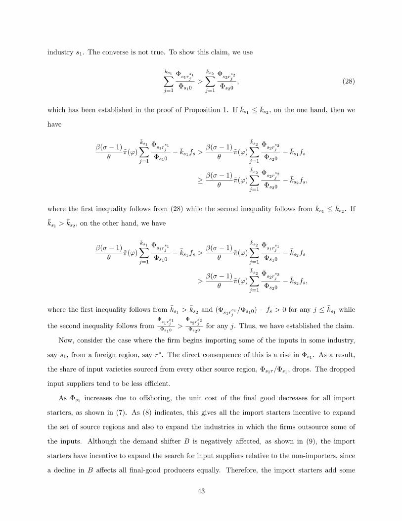
industry s1. The converse is not true. To show this claim, we use
ks1∑j=1
Φs1rs1j
Φs10>
ks2∑j=1
Φs2rs2j
Φs20, (28)
which has been established in the proof of Proposition 1. If ks1 ≤ ks2 , on the one hand, then we
have
β(σ − 1)
θπ(ϕ)
ks1∑j=1
Φs1rs1j
Φs10− ks1fs >
β(σ − 1)
θπ(ϕ)
ks2∑j=1
Φs2rs2j
Φs20− ks1fs
≥ β(σ − 1)
θπ(ϕ)
ks2∑j=1
Φs2rs2j
Φs20− ks2fs,
where the first inequality follows from (28) while the second inequality follows from ks1 ≤ ks2 . If
ks1 > ks2 , on the other hand, we have
β(σ − 1)
θπ(ϕ)
ks1∑j=1
Φs1rs1j
Φs10− ks1fs >
β(σ − 1)
θπ(ϕ)
ks2∑j=1
Φs1rs1j
Φs10− ks2fs
>β(σ − 1)
θπ(ϕ)
ks2∑j=1
Φs2rs2j
Φs20− ks2fs,
where the first inequality follows from ks1 > ks2 and (Φs1rs1j/Φs10) − fs > 0 for any j ≤ ks1 while
the second inequality follows fromΦs1r
s1j
Φs10>
Φs2r
s2j
Φs20for any j. Thus, we have established the claim.
Now, consider the case where the firm begins importing some of the inputs in some industry,
say s1, from a foreign region, say r∗. The direct consequence of this is a rise in Φs1 . As a result,
the share of input varieties sourced from every other source region, Φs1r/Φs1 , drops. The dropped
input suppliers tend to be less effi cient.
As Φs1 increases due to offshoring, the unit cost of the final good decreases for all import
starters, as shown in (7). As (8) indicates, this gives all the import starters incentive to expand
the set of source regions and also to expand the industries in which the firms outsource some of
the inputs. Although the demand shifter B is negatively affected, as shown in (9), the import
starters have incentive to expand the search for input suppliers relative to the non-importers, since
a decline in B affects all final-good producers equally. Therefore, the import starters add some
43
regions to the set of source regions for some industries, while they drop, as a consequence, ineffi cient
suppliers from all the existing source regions in those industries. Since newly-added regions are
associated with the smallest sourcing potentials compared with the existing source regions within
the industries, the newly-added sellers tend to be distantly located and more productive. If an
import starter begins outsourcing some of the inputs in an industry, then we know from the above
claim that the industry produces the most differentiated inputs of all the industries in which the
firm outsources. Proposition 1 tells us that the sellers in that industry tend to be closer than sellers
in other industries. This ends the proof of Proposition 2.
A.4.3 Proposition 3
Proposition 3 and the discussion that follows claim that if the fixed costs of outsourcing and
those of searching regions for input suppliers are large, the offshoring tend to result in industry
coagglomeration.
Proposition 2 shows that firms tend to offshore less differentiated inputs. Those inputs tend to
be outsourced from distant regions, so import starters tend to replace distant suppliers with foreign
sellers. Thus, the direct displacement induces industry coagglomeration. Proposition 2 also shows
two indirect channels through which the average distance between buyers and sellers is affected.
The first channel is the within-industry restructuring effect. Import starters tend to add suppliers in
distant regions while dropping firms in every existing source regions, so that the reshuffl ing induces
dispersion within the industries. The other channel, however, is for industry coagglomeration. It
is the channel of adding new ones in the list of the outsourcing industries, which we have referred
to as the industry composition effect. As we have seen, such industries tend to produce the more
differentiated inputs, and hence the sellers, which are newly-added, are located closer than those
in other industries on average.
If f and fs are large, the indirect effect tends to be for industry coagglomeration, since then the
number of outsourcing industries is small so that the dispersion effect is relatively small. In addition,
the indirect effect itself becomes small relative to the direct effect, since the import starters tend
to expand the search for new input suppliers less aggressively in that case, as we can see from (8).
Thus, if f and fs are large enough, offshoring induces industry coagglomeration. This completes
the proof of Proposition 3.
44

B Appendix for the Empirical Analysis
B.1 Measures of Industry Characteristics
Elasticity of Substitution
Source: Soderbery (2015). Description: refined estimates of the demand elasticity of U.S. im-
ported varieties (1993-2007), originally constructed by Broda and Weinstein (2006). Since product
categories are originally classified at the HS 6-digit, we use the following procedures to construct
the elasticity measure for each Japan’s Standard Industrial Classification (JSIC) 3-digit industry.
1. We first keep only intermediate inputs in the data set, based on the United Nations Broad
Economic Categories (BEC) list.
2. We then merge the list of intermediate inputs at the HS 6-digit level (2617 categories) with
the industry list of the Japanese Input-Output (IO) Table from 2005 (361 categories), using
the concordance file from the Statistics Bureau of Japan. The mapping is not unique– an HS
code can be mapped to multiple IO industry code, and vice versa.
3. We then map each IO code to a JSIC 4-digit code, using the concordance file from the
Statistics Bureau of Japan.
4. To construct the elasticity measure at the JSIC 3-digit and the broad BSJBSA sectors (12
manufacturing product groups), we compute the weighted average of ρs/ (ρs − 1) across all
corresponding 4-digit categories, with weights equal to the share of each 4-digit category in
the total sales of the 3-digit and BSJBSA broad sector, respectively. Sales data by 4-digit
industry for 2005 are obtained from the Census of Manufactures published from the Ministry
of Economy, Trade and Industry (METI).
5. We obtain 144 elasticity measures for 2005 (out of 150 JSIC (rev. 11) 3-digit manufacturing
industries), and 150 elasticity measures for 2010 (out of 177 JSIC2007 (rev. 12) manufacturing
industries).
Product Differentiation
Source: Rauch (1999). Description: a dummy variable that takes value equal to 1 for differ-
entiated products, and 0 for homogeneous products. There are two versions of the differentiation
45

indicator– “conservative” and “liberal”. In the main regressions, we use the “conservative” ver-
sion, which has a lower number of commodities classified as either organized exchange or reference
priced. Since industries are originally defined at the 4-digit level based on the ISIC (revision 3)
classification, we use the following procedures to construct the differentiation dummies for each
JSIC 3-digit category.53
1. We first map each ISIC 4-digit code (292 categories) to multiple JSIC (rev. 11) 4-digit codes
(1261 categories, with 563 manufacturing industries), using the concordance file from the
Statistics Bureau of Japan. Since the matching is many-to-one, we use the simple average of
the Rauch indicator across all ISIC codes within each JSIC. To define the Rauch dummy at
the JSIC level, we replace the computed averages that are strictly greater than 0.5 with 1,
and 0 otherwise.
2. To construct the Rauch differentiation indicator for a JSIC 3-digit industry or a broad
BSJBSA sector (one of twelve manufacturing product groups), we compute the weighted
average of the indicators across all affi liated 4-digit codes, with the weight equal to the share
of each 4-digit code in the total sales of the 3-digit or the BSJBSA sector, respectively. Data
on sales by 4-digit industry for 2005 are obtained from the Census of Manufactures from the
Ministry of Economy, Trade and Industry (METI). Once again, we replace the computed
averages that are strictly greater than 0.5 with 1, and 0 otherwise.
3. For 2005, we obtain 148 Rauch dummies (out of 150 possible JSIC (rev. 11) 3-digit manufac-
turing industries); while for 2010, we obtain 153 Rauch dummies (out of 177 possible JSIC
(rev. 12) manufacturing industries).
Air Freight Cost
Source: Hummels and Shaur (2013). Description: the cost of air freight for imports in each
U.S. industry, measured in ad-valorem terms (i.e., the percentage of the total value of shipment).
Purpose: We use it as a proxy for the timeliness of trade for each product. The concordance
procedure is identical to that used to construct the elasticity measures, as the air-freight measure
53According to the offi cial document by Japan’s Statistics Bureau, there are 420 3-digit categories and 1269 4-digitcategories for the JSIC2002 (Revision 11). For JSIC2007 (Revision 12), there are 529 3-digit categories and 14554-digit categories.
46
is originally available at the HS 6-digit (2002) level. 180 and 188 air-freight measures are available
for 2005 and 2010, respectively, at the JSIC 3-digit level.
B.2 Construction of the Instrument
To compute the growth rate of global exports at the JSIC 3-digit level, we first compute the
US dollar value of global exports to all countries expect Japan at the SITC (revision 2) 5-digit
level using Comtrade data (2005-2010). We then use a concordance file from the United Nations
Statistical Division to match a unique HS 4-digit (2002 version) category to a unique SITC code.
The unique match is determined based on the number of HS 10-digit categories shared between
a pair of SITC and HS code. For a handful of cases that a unique match cannot be determined
because there are multiple pairs that tie in terms of the number of HS 10-digit categories shared,
we will pick the smaller SITC in terms of the numeral value, albeit arbitrarily. Since a SITC may
be split into multiple HS 4-digit category, we will split the export value of a SITC category using
the number of HS 10-digit categories shared with each HS 4-digit as weight. We then repeat the
same procedure to match export values at the HS 4-digit levels to each IO code (361 of them), using
the concordance file from the Statistics Bureau of Japan, and finally map export values from IO
categories to JSIC (rev. 11) 4-digit categories, using another concordance file from the Statistics
Bureau. We then construct a firm-level instrument as specified in Equations (17) and (18) in the
main text.
47

B.3 New Method to Estimate the Dispersion of Firm Productivity (θ)
Firm i’s revenue can be written as R(zi) = Azρ−1i , where A is a constant that is common across all
firms in the industry.54 The distribution of a firm’s revenue, R, can be written as
G(R) = ProbRi < R
= ProbAzρ−1i < R
= Probzi < (R/A)1ρ−1
= F(
(R/A)1ρ−1
)= e−TA
θρ−1R
θ1−ρ
,
where F denotes the cumulative distribution function of Fréchet(T ,θ), implying that R is also
distributed Fréchet with the location parameter equal to T ′ = TAθρ−1 and the shape parameter
equal to θ′ = θ/(ρ− 1).
Now, the mean and variance of Frechet is given by
µ =1
T ′Γ
(1− 1
θ′
),
σ2 =1
T ′2
[Γ
(1− 2
θ′
)− Γ
(1− 1
θ′
)2],
where Γx =∫∞
0 tx−1e−tdt is the gamma function.
Consequently, we haveσ2
µ2=
Γ(1− 2
θ′)
Γ(1− 1
θ′)2 − 1.
Using Mathematica, we can identify θ′ using σ2 and µ2 for each 3-digit JSIC industry, each com-
puted using firm revenue data from TSR Company Information Database. Given estimates of ρs
from Soderbery (2015), we can then compute θs as (ρs − 1)θ′s, for each industry s.
54A =
(ρρ−1wc
P
)1−ρE.
48

References
[1] Acemoglu, D., V. M. Carvalho, A. Ozdaglar, and A. Tahbaz-Salehi (2012) “The Network
Origins of Aggregate Fluctuations”, Econometrica, 80(5), 1977-2016.
[2] Amiti, M. O. Itskhoki and J. Konings (2014) “Importers, Exporters and Exchange Rate Dis-
connect”, American Economic Review, 104(7): 1942-1978.
[3] Antràs, P. (2015). Global Production: Firms, Contracts, and Trade Structure. Princeton Uni-
versity Press.
[4] Antràs, P., T.C. Fort, and F. Tintelnot (2017), “The Margins of Global Sourcing: Theory and
Evidence from U.S. Firms”, American Economic Review, 107(9): 2514—2564.
[5] Atalay, E., A. Hortacsu, J. Roberts, and C. Syverson (2011) “Network Structure of Produc-
tion.”Proceedings of the National Academy of Sciences, 108(13), 5199-5202.
[6] Autor, D., H., Dorn, D., & Hanson, G.H. (2013) “The China Syndrome: Local Labor Market
Effects of Import Competition in the United States.” American Economic Review, 103(6),
2121-2168.
[7] Baldwin, R. and J. Harrigan (2011) “Zeros, Quality, and Space: Trade Theory and Trade
Evidence.”American Economic Journal: Microeconomics, 3 (May): 60-88.
[8] Baldwin, R. (2013) “Trade and Industrialization after Globalization’s Second Unbundling:
How Building and Joining a Supply Chain are Different and Why It Matters.”In Globalization
in an age of crisis: Multilateral economic cooperation in the twenty-first century (pp. 165-212).
University of Chicago Press.
[9] Banerjee, A. and E. Duflo (2000) “Reputation Effects and the Limits of Contracting: A Study
of the Indian Software Industry,”Quarterly Journal of Economics, 115: 989-1017.
[10] Bastos, P., J. Silva, and E. Verhoogen (2016) “Export Destinations and Input Prices.”
Columbia University Working Paper.
[11] Behrens, K. and T. Bougna (2015) “An Anatomy of the Geographical Concentration of Cana-
dian Manufacturing Industries.”Regional Science and Urban Economics, 51, 47-69.
49

[12] Bernard A.B., J.B. Jensen, S.J. Redding, P.K. Schott (2016) “Global Firms.”NBER Working
Paper No. 22727.
[13] Bernard, A.B., A. Moxnes and K.H. Ulltveit-Moe (2017) “Two-sided Heterogeneity and
Trade.”Dartmouth University Working Paper.
[14] Bernard, A.B., A. Moxnes and Y. Saito (2016) “Production Networks, Geography and Firm
Performance.”Dartmouth University Working Paper.
[15] Broda, C. and D. Weinstein (2006) “Globalization and the Gains from Variety.”Quarterly
Journal of Economics.
[16] Blaum, J., M. Peters and C. Lelarge (2016) “The Gains from Input Trade in Firm-Based
Models of Importing”, Yale University Working Paper.
[17] Blum, B.S., S. Claro, and I. J. Horstmann (2013) “Occasional and Perennial Exporters.”
Journal of International Economics, 90, no. 1: 65-74.
[18] Caliendo, L., and F. Parro (2015) “Estimates of the Trade and Welfare Effects of NAFTA.”
Review of Economic Studies, 82 (1): 1-44.
[19] Carballo, J., Ottaviano, G. I., & Volpe Martincus, C. (2016) “The Buyer Margins of Firms’
Exports.”CEP Discussion Paper No 1234.
[20] Carvalho, V. M., Nirei, M., Saito, Y. U., & Tahbaz-Salehi, A. (2017). “Supply Chain Disrup-
tions: Evidence from the Great East Japan Earthquake.”Northwestern University Working
Paper.
[21] Carvalho, V. and X. Gabaix (2013) “The Great Diversification and Its Undoing.”American
Economic Review, 2013, vol. 103(5), 1697-1727.
[22] Chaney, T. (2014) “The Network Structure of International Trade.”American Economic Re-
view, 104(11), 3600-3634.
[23] Chaney, T. (2016) “Networks in International Trade”, Oxford Handbook of the Economics of
Networks, ed. by Bramoulle, Galleoti and Rogers, Oxford University Press.
50

[24] Costinot, A. and A. Rodriguez-Clare (2014) “Trade Theory with Numbers: Quantifying the
Consequences of Globalization”, Handbook of International Economics, 2014, Volume 4, Chap-
ter 4, Gita Gopinath, Elhanan Helpman, and Kenneth Rogoff editors.
[25] Cristea, A.D. (2011) “Buyer-Seller Relationships in International Trade: Evidence from U.S.
States’Exports and Business-Class Travel”, Journal of International Economics, 84(2): 207—
220.
[26] Davis, D.R. and J.I. Dingel (2016) “A Spatial Knowledge Economy”, University of Chicago
Working Paper.
[27] Davis, S.J., J.C. Haltiwanger, and S. Shuh (1998) Job Creation and Destruction, MIT Press.
[28] Dumais, G., G.E. Ellison, and E.L. Glaeser (2002) “Geographic Concentration as a Dynamic
Process.”Review of Economics and Statistics, 84, 193-204.
[29] Eaton, J., Eslava, M., Krizan, C. J., Kugler, M., & Tybout, J. (2014) “A Search and Learning
Model of Export Dynamics.”Penn State University mimeo.
[30] Eaton, J. and S. Kortum (2002) “Technology, Geography, and Trade”, Econometrica, 70,
1741-1779.
[31] Ebenstein, A., Harrison, A., McMillan, M., and Phillips, S. (2014). “Estimating the Impact of
Trade and Offshoring on American Workers Using the Current Population Surveys.”Review
of Economics and Statistics, 96(4), 581-595.
[32] Ellison, G. and E.L. Glaeser (1997) “Geographic Concentration in U.S. Manufacturing Indus-
tries: A Dartboard Approach.”Journal of Political Economy, 105, 889-927.
[33] Ellison, G., E.L. Glaeser, and W.R. Kerr (2010) “What Causes Industry Agglomeration?
Evidence from Coagglomeration Patterns.”American Economic Review, 100, 1195-1213.
[34] Feenstra R. (2008) “Offshoring in the Global Economy”, Ohlin Lectures.
[35] Hallak, J. and J. Sivadasan (2013) “Product and Process Productivity: Implications for Quality
Choice and Conditional Exporter Premia”, Journal of International Economics, 91(1), pp. 53-
67.
51

[36] Hijzen, A, T. Inui, and Y. Todo (2010) “Does Offshoring Pay? Firm-Level Evidence from
Japan.”Economic Inquiry, 48(4), 880—895.
[37] Harvard Business Review. (2009) “Managing across Distance in Today’s Economic Climate:
The Value of Face-to-Face Communication.”Harvard Business School Publishing
[38] Holmes, T. and J. Stevens (2014) “An Alternative Theory of the Plant Size Distribution with
Geography and Intra- and International Trade,”Journal of Political Economy, vol. 122, no. 2.
[39] Hummels, D., R. Jorgensen, J.R. Munch, and C. Xiang (2014) “The Wage Effects of Offshoring:
Evidence from Danish Matched Worker-firm Data.”American Economic Review, 104(6): 1597-
1629.
[40] Hummels, D.L. and G. Schaur (2013) “Time as a Trade Barrier.”American Economic Review,
Vol. 103, No. 7, pp. 2935-59.
[41] Jensen, J.B., and L.G. Kletzer (2005) “Tradable Services: Understanding the Scope and Impact
of Services Offshoring.”Brookings Trade Forum 2005: 75-116.
[42] Johnson, R.C. and G. Noguera (2016) “A Portrait of Trade in Value Added over Four Decades”
Review of Economics and Statistics, forthcoming.
[43] Jones, C. (2011) “Intermediate Goods and Weak Links in the Theory of Economic Develop-
ment”American Economic Journal: Macroeconomics, 3(2), 1-28.
[44] Jones, C. (2013) “Misallocation, Economic Growth, and Input-Output Economics”in Advances
in Economics and Econometrics, Tenth World Congress, Volume II, Cambridge University
Press.
[45] Javorcik, Beata S. (2004) “Does Foreign Direct Investment Increase the Productivity of Domes-
tic Firms? In Search of Spillovers Through Backward Linkages”American Economic Review,
94(3), pp. 605-627.
[46] Kasahara, H., and Rodrigue, J. (2008). "Does the Use of Imported Intermediates Increase
Productivity? Plant-level Evidence." Journal of Development Economics, 87 (1), 106-118.
52

[47] Keller, W., and S.R. Yeaple (2013) “The Gravity of Knowledge.”American Economic Review,
103(4), 1414-1444.
[48] Khandelwal, A. (2010) “The Long and Short (of) Quality Ladders.” Review of Economic
Studies, 77 (4), 1450-1476.
[49] Kremer, M. (1993) “The O-ring Theory of Economic Development.” Quarterly Journal of
Economics, 108 (3), 551-575.
[50] Lerner, J. (1995) “Venture Capitalists and the Oversight of Private Firms.”Journal of Finance,
50, 1: 301-318.
[51] Lim, K. (2017) “Firm-to-firm Trade in Sticky Production Networks.”University of Toronto
Working Paper.
[52] Liu, R., B. Scholnick, and A. Finn (2017) “The Complexity of Outsourced Services and the
Role of International Business Travel.”Journal of Economic Geography, 17, pp. 661—684.
[53] Nakajima, K., Y. Saito, and I. Uesugi (2012) "Measuring Economic Localization: Evidence
from Japanese Firm-Level Data," Journal of the Japanese and International Economies 26
(2): 201-220.
[54] Oberfield, E. (2017) “A Theory of Input-Output Architecture.”Princeton University, mimeo.
[55] Petersen, M.A., and R.G. Rajan (2002) “Does Distance Still Matter? The Information Revo-
lution in Small Business Lending.”Journal of Finance, 57 (6), 2533—2570.
[56] Rauch, J. (1999) “Networks versus Markets in International Trade.”Journal of International
Economics, 48, 7—35.
[57] Rauch, J. and Trindade, V. (2002) “Ethnic Chinese Networks in International Trade.”Review
of Economics and Statistics, 84 (1), 116—130.
[58] Redding, S.J. and E. Rossi-Hansberg (2016) “Quantitative Spatial Economics.” Princeton
University Working Paper.
[59] Rosenthal, Stuart S. and William C. Strange (2001) “The Determinants of Agglomeration.”
Journal of Urban Economics, 50, 191-229.
53
[60] Soderbery, A. (2015) “Estimating Import Supply and Demand Elasticities: Analysis and Im-
plications.”Journal of International Economics, 96(1), pp 1-17.
[61] Sugita, Y., Teshima, K., Seira, E. (2017) “Assortative Matching of Exporters and Importers.”
RIETI Discussion Paper Series 17-E-016.
[62] Tintelnot, F., A. Kikkawa, M. Mogstad, and E. Dhyne (2017) “Trade and Domestic Production
Networks.”University of Chicago Working Paper.
[63] Wooldridge, J. M. (2010). Econometric Analysis of Cross Section and Panel Data. MIT press.
[64] World Trade Organization (2013) World Trade Report 2013: Factors Shaping the Future of
World Trade.
54
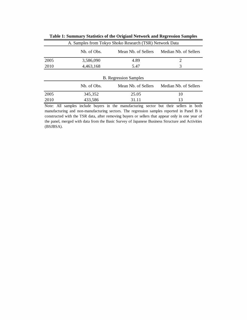
2005 3,586,090 4.89 22010 4,463,168 5.47 3
2005 345,352 25.05 102010 433,586 31.11 13Note: All samples include buyers in the manufacturing sector but their sellers in bothmanufacturing and non-manufacturing sectors. The regression samples reported in Panel B isconstructed with the TSR data, after removing buyers or sellers that appear only in one year ofthe panel, merged with data from the Basic Survey of Japanese Business Structure and Activities(BSJBSA).
A. Samples from Tokyo Shoko Research (TSR) Network DataTable 1: Summary Statistics of the Origianl Network and Regression Samples
Nb. of Obs. Mean Nb. of Sellers Median Nb. of Sellers
B. Regression Samples
Nb. of Obs. Mean Nb. of Sellers Median Nb. of Sellers
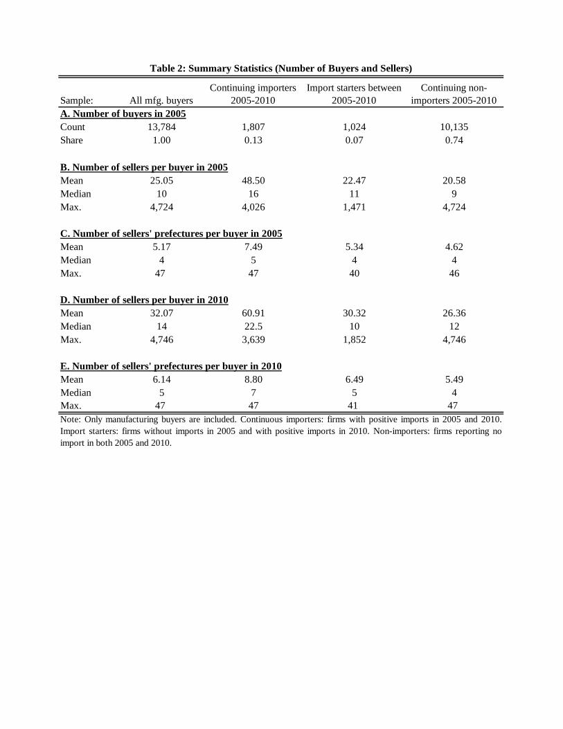
Count 13,784 1,807 1,024 10,135Share 1.00 0.13 0.07 0.74
Mean 25.05 48.50 22.47 20.58Median 10 16 11 9Max. 4,724 4,026 1,471 4,724
Mean 5.17 7.49 5.34 4.62Median 4 5 4 4Max. 47 47 40 46
Mean 32.07 60.91 30.32 26.36Median 14 22.5 10 12Max. 4,746 3,639 1,852 4,746
Mean 6.14 8.80 6.49 5.49Median 5 7 5 4Max. 47 47 41 47
A. Number of buyers in 2005
Note: Only manufacturing buyers are included. Continuous importers: firms with positive imports in 2005 and 2010.Import starters: firms without imports in 2005 and with positive imports in 2010. Non-importers: firms reporting noimport in both 2005 and 2010.
D. Number of sellers per buyer in 2010
C. Number of sellers' prefectures per buyer in 2005
E. Number of sellers' prefectures per buyer in 2010
B. Number of sellers per buyer in 2005
Table 2: Summary Statistics (Number of Buyers and Sellers)
All mfg. buyersContinuing importers
2005-2010Import starters between
2005-2010Continuing non-
importers 2005-2010Sample:
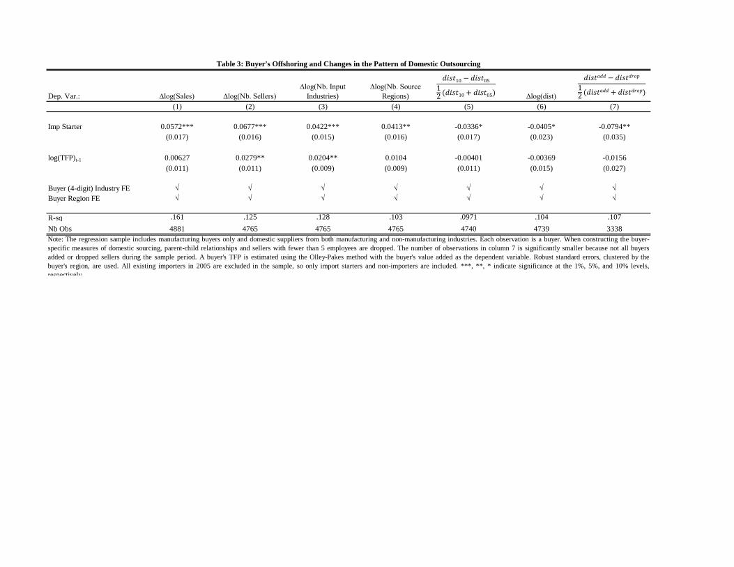
Dep. Var.: ∆log(Sales) ∆log(Nb. Sellers)∆log(Nb. Input
Industries)∆log(Nb. Source
Regions) ∆log(dist)(1) (2) (3) (4) (5) (6) (7)
Imp Starter 0.0572*** 0.0677*** 0.0422*** 0.0413** -0.0336* -0.0405* -0.0794**(0.017) (0.016) (0.015) (0.016) (0.017) (0.023) (0.035)
log(TFP)t-1 0.00627 0.0279** 0.0204** 0.0104 -0.00401 -0.00369 -0.0156(0.011) (0.011) (0.009) (0.009) (0.011) (0.015) (0.027)
Buyer (4-digit) Industry FE √ √ √ √ √ √ √Buyer Region FE √ √ √ √ √ √ √
R-sq .161 .125 .128 .103 .0971 .104 .107Nb Obs 4881 4765 4765 4765 4740 4739 3338Note: The regression sample includes manufacturing buyers only and domestic suppliers from both manufacturing and non-manufacturing industries. Each observation is a buyer. When constructing the buyer-specific measures of domestic sourcing, parent-child relationships and sellers with fewer than 5 employees are dropped. The number of observations in column 7 is significantly smaller because not all buyersadded or dropped sellers during the sample period. A buyer's TFP is estimated using the Olley-Pakes method with the buyer's value added as the dependent variable. Robust standard errors, clustered by thebuyer's region, are used. All existing importers in 2005 are excluded in the sample, so only import starters and non-importers are included. ***, **, * indicate significance at the 1%, 5%, and 10% levels,respectively
Table 3: Buyer's Offshoring and Changes in the Pattern of Domestic Outsourcing
𝑑𝑑𝑑𝑑10 − 𝑑𝑑𝑑𝑑0512 (𝑑𝑑𝑑𝑑10 + 𝑑𝑑𝑑𝑑05)
𝑑𝑑𝑑𝑑𝑎𝑑𝑑 − 𝑑𝑑𝑑𝑑𝑑𝑑𝑑𝑑
12 (𝑑𝑑𝑑𝑑𝑎𝑑𝑑 + 𝑑𝑑𝑑𝑑𝑑𝑑𝑑𝑑)
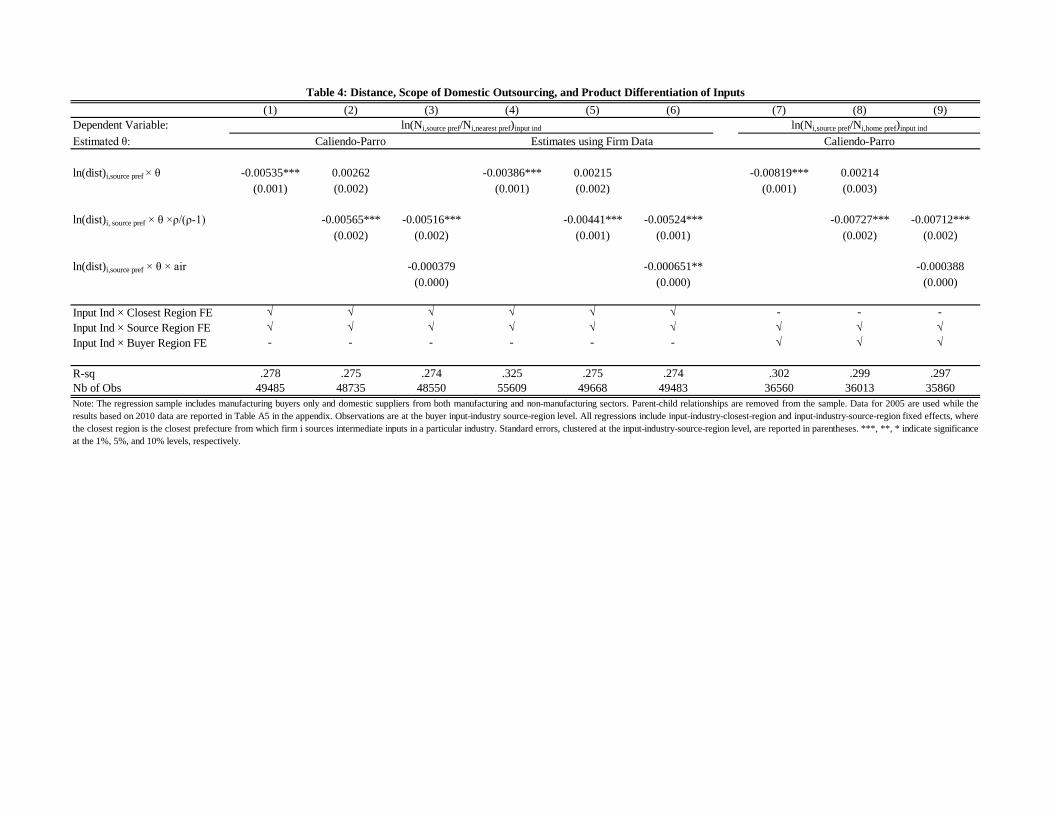
(1) (2) (3) (4) (5) (6) (7) (8) (9)Dependent Variable:Estimated θ:
ln(dist)i,source pref × θ -0.00535*** 0.00262 -0.00386*** 0.00215 -0.00819*** 0.00214(0.001) (0.002) (0.001) (0.002) (0.001) (0.003)
ln(dist)i, source pref × θ ×ρ/(ρ-1) -0.00565*** -0.00516*** -0.00441*** -0.00524*** -0.00727*** -0.00712***(0.002) (0.002) (0.001) (0.001) (0.002) (0.002)
ln(dist)i,source pref × θ × air -0.000379 -0.000651** -0.000388(0.000) (0.000) (0.000)
Input Ind × Closest Region FE √ √ √ √ √ √ - - -Input Ind × Source Region FE √ √ √ √ √ √ √ √ √Input Ind × Buyer Region FE - - - - - - √ √ √
R-sq .278 .275 .274 .325 .275 .274 .302 .299 .297Nb of Obs 49485 48735 48550 55609 49668 49483 36560 36013 35860
Caliendo-Parro
Note: The regression sample includes manufacturing buyers only and domestic suppliers from both manufacturing and non-manufacturing sectors. Parent-child relationships are removed from the sample. Data for 2005 are used while theresults based on 2010 data are reported in Table A5 in the appendix. Observations are at the buyer input-industry source-region level. All regressions include input-industry-closest-region and input-industry-source-region fixed effects, wherethe closest region is the closest prefecture from which firm i sources intermediate inputs in a particular industry. Standard errors, clustered at the input-industry-source-region level, are reported in parentheses. ***, **, * indicate significanceat the 1%, 5%, and 10% levels, respectively.
Table 4: Distance, Scope of Domestic Outsourcing, and Product Differentiation of Inputs
ln(Ni,source pref/Ni,home pref)input indln(Ni,source pref/Ni,nearest pref)input ind
Caliendo-Parro Estimates using Firm Data
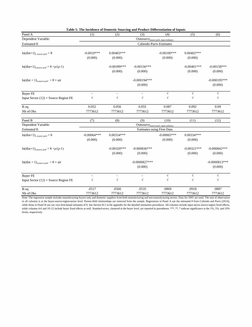
Panel A (1) (2) (3) (4) (5) (6)Dependent Variable:Estimated θ:
ln(dist+1)i, source pref × θ -0.0010*** 0.00403*** -0.00100*** 0.00402***(0.000) (0.000) (0.000) (0.000)
ln(dist+1)i,source pref × θ ×ρ/(ρ-1) -0.00399*** -0.00156*** -0.00401*** -0.00158***(0.000) (0.000) (0.000) (0.000)
ln(dist + 1)i,source pref × θ × air -0.000194*** -0.000195***(0.000) (0.000)
Buyer FE - - - √ √ √Input Sector (12) × Source Region FE √ √ √ √ √ √
R-sq 0.052 0.056 0.055 0.087 0.092 0.09Nb of Obs 7773612 7773612 7773612 7773612 7773612 7773612
Panel B (7) (8) (9) (10) (11) (12)Dependent Variable:Estimated θ:
ln(dist+1)i, source pref × θ -0.00064*** 0.00334*** -0.00065*** 0.00334***(0.000) (0.000) (0.000) (0.000)
ln(dist+1)i,source pref × θ ×ρ/(ρ-1) -0.00320*** -0.000836*** -0.00321*** -0.000842***(0.000) (0.000) (0.000) (0.000)
ln(dist + 1)i,source pref × θ × air -0.0000827*** -0.0000813***(0.000) (0.000)
Buyer FE - - - √ √ √Input Sector (12) × Source Region FE √ √ √ √ √ √
R-sq .0517 .0566 .0535 .0869 .0918 .0887Nb of Obs 7773612 7773612 7773612 7773612 7773612 7773612Note: The regression sample includes manufacturing buyers only and domestic suppliers from both manufacturing and non-manufacturing sectors. Data for 2005 are used. The unit of observationin all columns is at the buyer-source-region-sector level. Parent-child relationships are removed from the sample. Regressions in Panel A use the estimated θ from Caliendo and Parro (2014),while those in Panel B use our own firm-based estimates of θ. See Section B.5 in the appendix for the detailed estimation procedures. All columns include input-sector-source-region fixed effects,while columns 4-6 and 10-12 include buyer fixed effects as well. Standard errors, clustered at the buyer level, are reported in parentheses. ***, **, * indicate significance at the 1%, 5%, and 10%levels, respectively.
Caliendo-Parro Estimates
Estimates using Firm Data
Table 5: The Incidence of Domestic Sourcing and Product Differentiation of Inputs
Outsourcesource pref, input industry
Outsourcesource pref, input industry
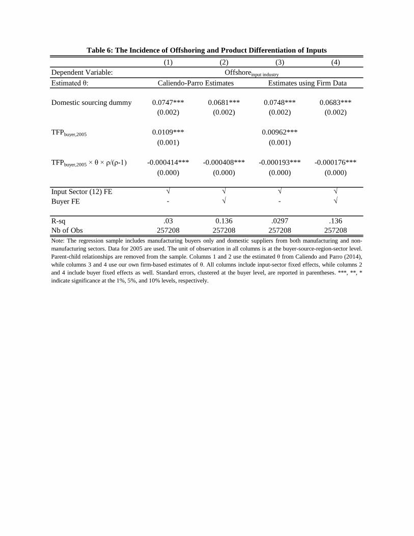
(1) (2) (3) (4)Dependent Variable:Estimated θ:
Domestic sourcing dummy 0.0747*** 0.0681*** 0.0748*** 0.0683***(0.002) (0.002) (0.002) (0.002)
TFPbuyer,2005 0.0109*** 0.00962***(0.001) (0.001)
TFPbuyer,2005 × θ × ρ/(ρ-1) -0.000414*** -0.000408*** -0.000193*** -0.000176***(0.000) (0.000) (0.000) (0.000)
Input Sector (12) FE √ √ √ √Buyer FE - √ - √
R-sq .03 0.136 .0297 .136Nb of Obs 257208 257208 257208 257208Note: The regression sample includes manufacturing buyers only and domestic suppliers from both manufacturing and non-manufacturing sectors. Data for 2005 are used. The unit of observation in all columns is at the buyer-source-region-sector level.Parent-child relationships are removed from the sample. Columns 1 and 2 use the estimated θ from Caliendo and Parro (2014),while columns 3 and 4 use our own firm-based estimates of θ. All columns include input-sector fixed effects, while columns 2and 4 include buyer fixed effects as well. Standard errors, clustered at the buyer level, are reported in parentheses. ***, **, *indicate significance at the 1%, 5%, and 10% levels, respectively.
Offshoreinput industry
Caliendo-Parro Estimates Estimates using Firm Data
Table 6: The Incidence of Offshoring and Product Differentiation of Inputs
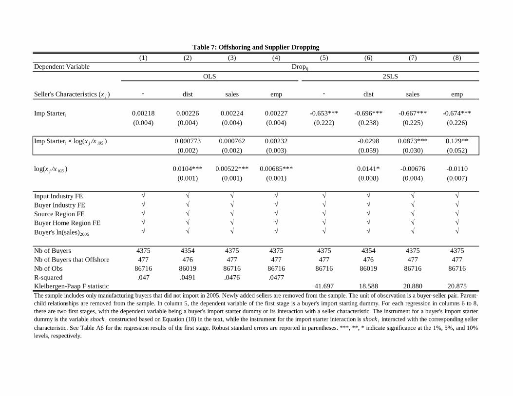
(1) (2) (3) (4) (5) (6) (7) (8)Dependent Variable
Seller's Characteristics (x j ) - dist sales emp - dist sales emp
Imp Starteri 0.00218 0.00226 0.00224 0.00227 -0.653*** -0.696*** -0.667*** -0.674***(0.004) (0.004) (0.004) (0.004) (0.222) (0.238) (0.225) (0.226)
Imp Starteri × log(x j /x i05 ) 0.000773 0.000762 0.00232 -0.0298 0.0873*** 0.129**(0.002) (0.002) (0.003) (0.059) (0.030) (0.052)
log(x j /x i05 ) 0.0104*** 0.00522*** 0.00685*** 0.0141* -0.00676 -0.0110(0.001) (0.001) (0.001) (0.008) (0.004) (0.007)
Input Industry FE √ √ √ √ √ √ √ √Buyer Industry FE √ √ √ √ √ √ √ √Source Region FE √ √ √ √ √ √ √ √Buyer Home Region FE √ √ √ √ √ √ √ √Buyer's ln(sales)2005 √ √ √ √ √ √ √ √
Nb of Buyers 4375 4354 4375 4375 4375 4354 4375 4375Nb of Buyers that Offshore 477 476 477 477 477 476 477 477Nb of Obs 86716 86019 86716 86716 86716 86019 86716 86716R-squared .047 .0491 .0476 .0477Kleibergen-Paap F statistic 41.697 18.588 20.880 20.875
Dropij
OLS 2SLS
The sample includes only manufacturing buyers that did not import in 2005. Newly added sellers are removed from the sample. The unit of observation is a buyer-seller pair. Parent-child relationships are removed from the sample. In column 5, the dependent variable of the first stage is a buyer's import starting dummy. For each regression in columns 6 to 8,there are two first stages, with the dependent variable being a buyer's import starter dummy or its interaction with a seller characteristic. The instrument for a buyer's import starterdummy is the variable shock i constructed based on Equation (18) in the text, while the instrument for the import starter interaction is shock i interacted with the corresponding sellercharacteristic. See Table A6 for the regression results of the first stage. Robust standard errors are reported in parentheses. ***, **, * indicate significance at the 1%, 5%, and 10%levels, respectively.
Table 7: Offshoring and Supplier Dropping
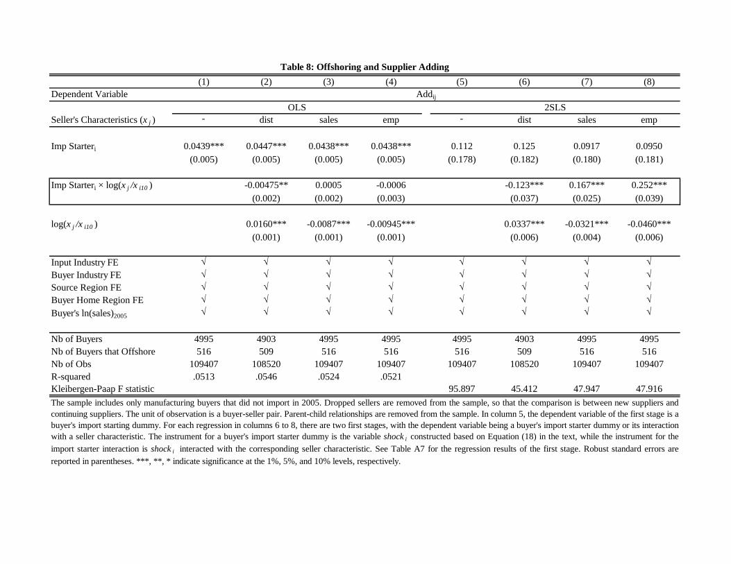
(1) (2) (3) (4) (5) (6) (7) (8)Dependent Variable
Seller's Characteristics (x j ) - dist sales emp - dist sales emp
Imp Starteri 0.0439*** 0.0447*** 0.0438*** 0.0438*** 0.112 0.125 0.0917 0.0950(0.005) (0.005) (0.005) (0.005) (0.178) (0.182) (0.180) (0.181)
Imp Starteri × log(x j /x i10 ) -0.00475** 0.0005 -0.0006 -0.123*** 0.167*** 0.252***(0.002) (0.002) (0.003) (0.037) (0.025) (0.039)
log(x j /x i10 ) 0.0160*** -0.0087*** -0.00945*** 0.0337*** -0.0321*** -0.0460***(0.001) (0.001) (0.001) (0.006) (0.004) (0.006)
Input Industry FE √ √ √ √ √ √ √ √Buyer Industry FE √ √ √ √ √ √ √ √Source Region FE √ √ √ √ √ √ √ √Buyer Home Region FE √ √ √ √ √ √ √ √Buyer's ln(sales)2005 √ √ √ √ √ √ √ √
Nb of Buyers 4995 4903 4995 4995 4995 4903 4995 4995Nb of Buyers that Offshore 516 509 516 516 516 509 516 516Nb of Obs 109407 108520 109407 109407 109407 108520 109407 109407R-squared .0513 .0546 .0524 .0521Kleibergen-Paap F statistic 95.897 45.412 47.947 47.916
OLS 2SLS
The sample includes only manufacturing buyers that did not import in 2005. Dropped sellers are removed from the sample, so that the comparison is between new suppliers andcontinuing suppliers. The unit of observation is a buyer-seller pair. Parent-child relationships are removed from the sample. In column 5, the dependent variable of the first stage is abuyer's import starting dummy. For each regression in columns 6 to 8, there are two first stages, with the dependent variable being a buyer's import starter dummy or its interactionwith a seller characteristic. The instrument for a buyer's import starter dummy is the variable shock i constructed based on Equation (18) in the text, while the instrument for theimport starter interaction is shock i interacted with the corresponding seller characteristic. See Table A7 for the regression results of the first stage. Robust standard errors arereported in parentheses. ***, **, * indicate significance at the 1%, 5%, and 10% levels, respectively.
Table 8: Offshoring and Supplier Adding
Addij
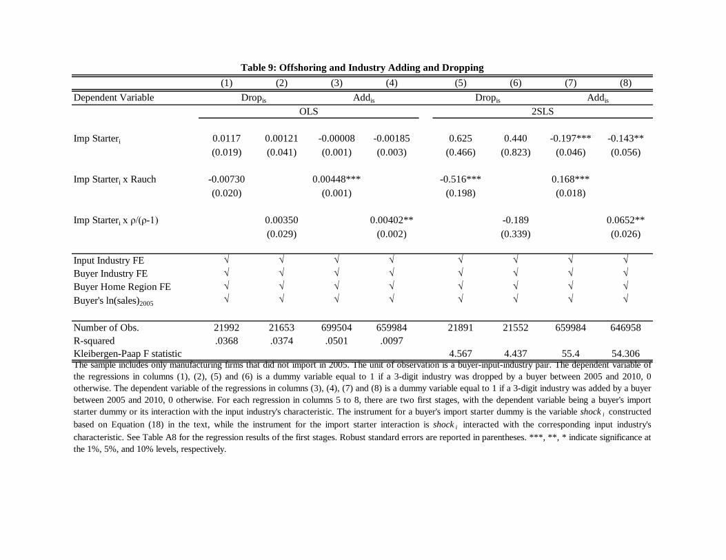
(1) (2) (3) (4) (5) (6) (7) (8)Dependent Variable
Imp Starteri 0.0117 0.00121 -0.00008 -0.00185 0.625 0.440 -0.197*** -0.143**(0.019) (0.041) (0.001) (0.003) (0.466) (0.823) (0.046) (0.056)
Imp Starteri x Rauch -0.00730 0.00448*** -0.516*** 0.168***(0.020) (0.001) (0.198) (0.018)
Imp Starteri x ρ/(ρ-1) 0.00350 0.00402** -0.189 0.0652**(0.029) (0.002) (0.339) (0.026)
Input Industry FE √ √ √ √ √ √ √ √Buyer Industry FE √ √ √ √ √ √ √ √Buyer Home Region FE √ √ √ √ √ √ √ √Buyer's ln(sales)2005 √ √ √ √ √ √ √ √
Number of Obs. 21992 21653 699504 659984 21891 21552 659984 646958R-squared .0368 .0374 .0501 .0097Kleibergen-Paap F statistic 4.567 4.437 55.4 54.306The sample includes only manufacturing firms that did not import in 2005. The unit of observation is a buyer-input-industry pair. The dependent variable ofthe regressions in columns (1), (2), (5) and (6) is a dummy variable equal to 1 if a 3-digit industry was dropped by a buyer between 2005 and 2010, 0otherwise. The dependent variable of the regressions in columns (3), (4), (7) and (8) is a dummy variable equal to 1 if a 3-digit industry was added by a buyerbetween 2005 and 2010, 0 otherwise. For each regression in columns 5 to 8, there are two first stages, with the dependent variable being a buyer's importstarter dummy or its interaction with the input industry's characteristic. The instrument for a buyer's import starter dummy is the variable shock i constructedbased on Equation (18) in the text, while the instrument for the import starter interaction is shock i interacted with the corresponding input industry'scharacteristic. See Table A8 for the regression results of the first stages. Robust standard errors are reported in parentheses. ***, **, * indicate significance atthe 1%, 5%, and 10% levels, respectively.
Table 9: Offshoring and Industry Adding and Dropping
2SLSOLSDropis Addis Dropis Addis
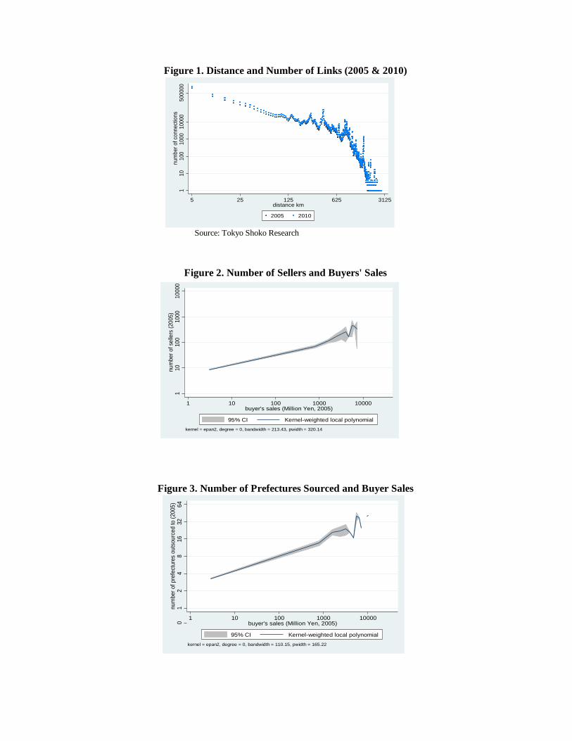
Figure 2. Number of Sellers and Buyers' Sales
Figure 3. Number of Prefectures Sourced and Buyer Sales
Figure 1. Distance and Number of Links (2005 & 2010)
Source: Tokyo Shoko Research
01
24
816
3264
num
ber o
f pre
fect
ures
out
sour
ced
to (2
005)
1 10 100 1000 10000buyer's sales (Million Yen, 2005)
95% CI Kernel-weighted local polynomial
kernel = epan2, degree = 0, bandwidth = 110.15, pwidth = 165.22
110
100
1000
1000
0nu
mbe
r of s
elle
rs (2
005)
1 10 100 1000 10000buyer's sales (Million Yen, 2005)
95% CI Kernel-weighted local polynomial
kernel = epan2, degree = 0, bandwidth = 213.43, pwidth = 320.14
110
100
1000
1000
050
0000
num
ber o
f con
nect
ions
5 25 125 625 3125distance km
2005 2010
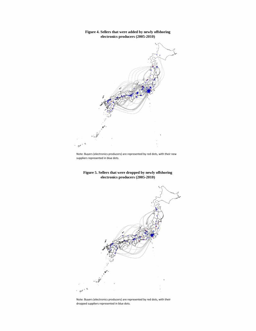
Figure 4. Sellers that were added by newly offshoring electronics producers (2005-2010)
Note: Buyers (electronics producers) are represented by red dots, with their new suppliers represented in blue dots.
Figure 5. Sellers that were dropped by newly offshoring electronics producers (2005-2010)
Note: Buyers (electronics producers) are represented by red dots, with their dropped suppliers represented in blue dots.
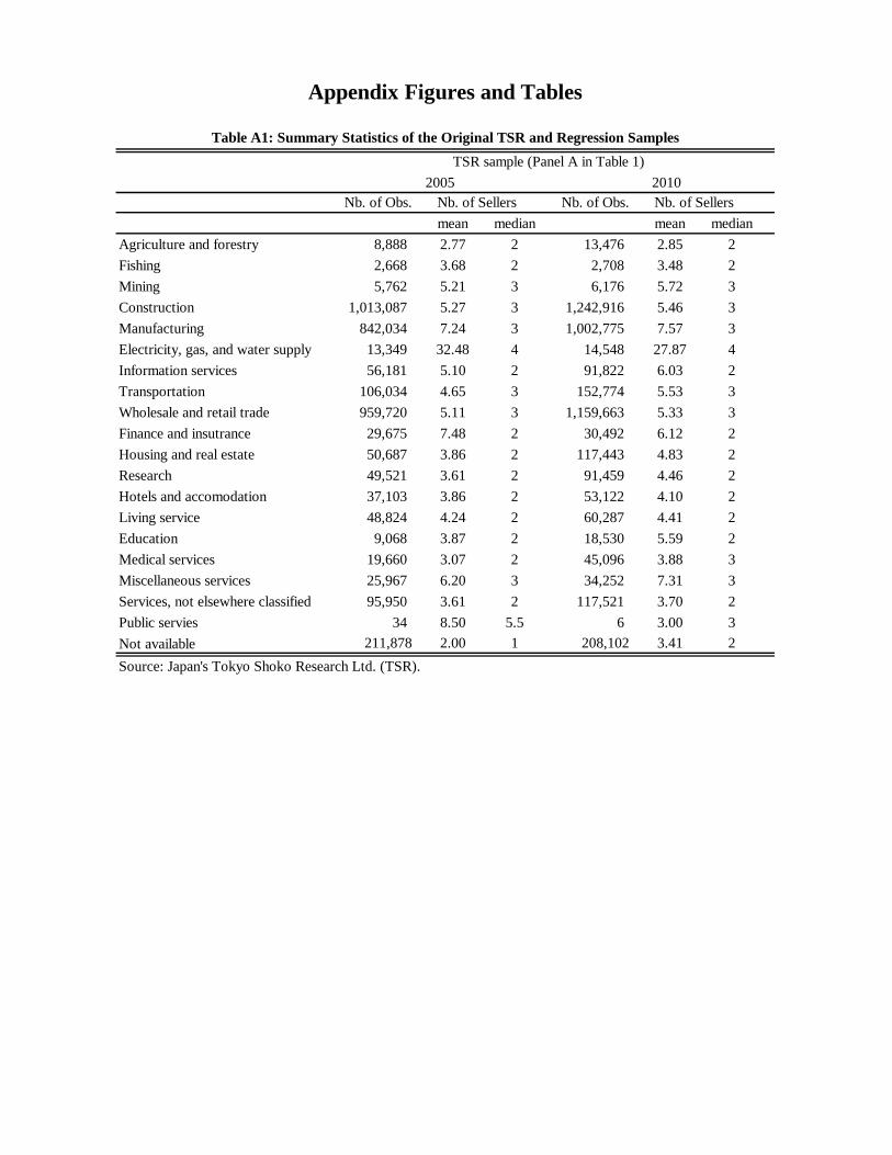
Nb. of Obs. Nb. of Obs.mean median mean median
Agriculture and forestry 8,888 2.77 2 13,476 2.85 2Fishing 2,668 3.68 2 2,708 3.48 2Mining 5,762 5.21 3 6,176 5.72 3Construction 1,013,087 5.27 3 1,242,916 5.46 3Manufacturing 842,034 7.24 3 1,002,775 7.57 3Electricity, gas, and water supply 13,349 32.48 4 14,548 27.87 4Information services 56,181 5.10 2 91,822 6.03 2Transportation 106,034 4.65 3 152,774 5.53 3Wholesale and retail trade 959,720 5.11 3 1,159,663 5.33 3Finance and insutrance 29,675 7.48 2 30,492 6.12 2Housing and real estate 50,687 3.86 2 117,443 4.83 2Research 49,521 3.61 2 91,459 4.46 2Hotels and accomodation 37,103 3.86 2 53,122 4.10 2Living service 48,824 4.24 2 60,287 4.41 2Education 9,068 3.87 2 18,530 5.59 2Medical services 19,660 3.07 2 45,096 3.88 3Miscellaneous services 25,967 6.20 3 34,252 7.31 3Services, not elsewhere classified 95,950 3.61 2 117,521 3.70 2Public servies 34 8.50 5.5 6 3.00 3Not available 211,878 2.00 1 208,102 3.41 2Source: Japan's Tokyo Shoko Research Ltd. (TSR).
Nb. of Sellers Nb. of Sellers2005 2010
Appendix Figures and Tables
Table A1: Summary Statistics of the Original TSR and Regression SamplesTSR sample (Panel A in Table 1)
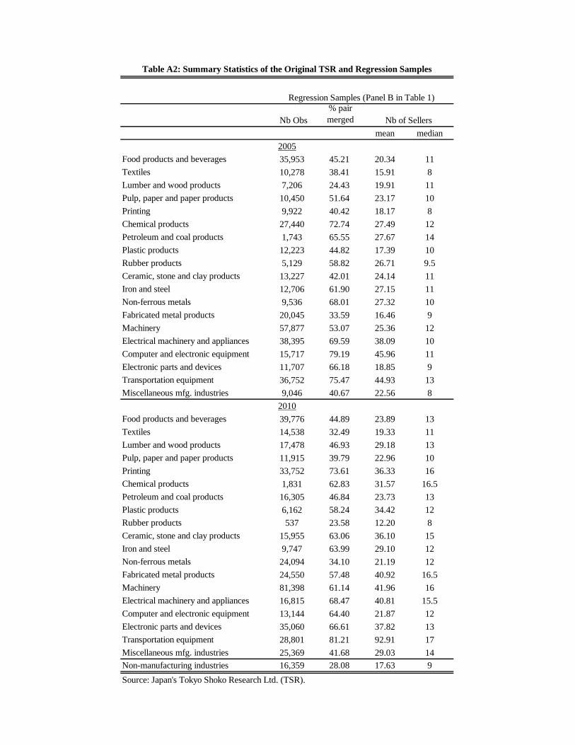
Nb Obs% pair merged
mean median
Food products and beverages 35,953 45.21 20.34 11Textiles 10,278 38.41 15.91 8Lumber and wood products 7,206 24.43 19.91 11Pulp, paper and paper products 10,450 51.64 23.17 10Printing 9,922 40.42 18.17 8Chemical products 27,440 72.74 27.49 12Petroleum and coal products 1,743 65.55 27.67 14Plastic products 12,223 44.82 17.39 10Rubber products 5,129 58.82 26.71 9.5Ceramic, stone and clay products 13,227 42.01 24.14 11Iron and steel 12,706 61.90 27.15 11Non-ferrous metals 9,536 68.01 27.32 10Fabricated metal products 20,045 33.59 16.46 9Machinery 57,877 53.07 25.36 12Electrical machinery and appliances 38,395 69.59 38.09 10Computer and electronic equipment 15,717 79.19 45.96 11Electronic parts and devices 11,707 66.18 18.85 9Transportation equipment 36,752 75.47 44.93 13Miscellaneous mfg. industries 9,046 40.67 22.56 8
Food products and beverages 39,776 44.89 23.89 13Textiles 14,538 32.49 19.33 11Lumber and wood products 17,478 46.93 29.18 13Pulp, paper and paper products 11,915 39.79 22.96 10Printing 33,752 73.61 36.33 16Chemical products 1,831 62.83 31.57 16.5Petroleum and coal products 16,305 46.84 23.73 13Plastic products 6,162 58.24 34.42 12Rubber products 537 23.58 12.20 8Ceramic, stone and clay products 15,955 63.06 36.10 15Iron and steel 9,747 63.99 29.10 12Non-ferrous metals 24,094 34.10 21.19 12Fabricated metal products 24,550 57.48 40.92 16.5Machinery 81,398 61.14 41.96 16Electrical machinery and appliances 16,815 68.47 40.81 15.5Computer and electronic equipment 13,144 64.40 21.87 12Electronic parts and devices 35,060 66.61 37.82 13Transportation equipment 28,801 81.21 92.91 17Miscellaneous mfg. industries 25,369 41.68 29.03 14Non-manufacturing industries 16,359 28.08 17.63 9Source: Japan's Tokyo Shoko Research Ltd. (TSR).
Regression Samples (Panel B in Table 1)
Nb of Sellers
Table A2: Summary Statistics of the Original TSR and Regression Samples
2010
2005
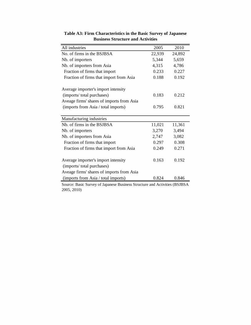
All industries 2005 2010No. of firms in the BSJBSA 22,939 24,892Nb. of importers 5,344 5,659Nb. of importers from Asia 4,315 4,786 Fraction of firms that import 0.233 0.227 Fraction of firms that import from Asia 0.188 0.192
Average importer's import intensity (imports/ total purchases) 0.183 0.212Aveage firms' shares of imports from Asia (imports from Asia / total imports) 0.795 0.821
Manufacturing industriesNb. of firms in the BSJBSA 11,021 11,361Nb. of importers 3,270 3,494Nb. of importers from Asia 2,747 3,082 Fraction of firms that import 0.297 0.308 Fraction of firms that import from Asia 0.249 0.271
Average importer's import intensity 0.163 0.192 (imports/ total purchases)Aveage firms' shares of imports from Asia (imports from Asia / total imports) 0.824 0.846
Table A3: Firm Characteristics in the Basic Survey of Japanese Business Structure and Activities
Source: Basic Survey of Japanese Business Structure and Activities (BSJBSA 2005, 2010)
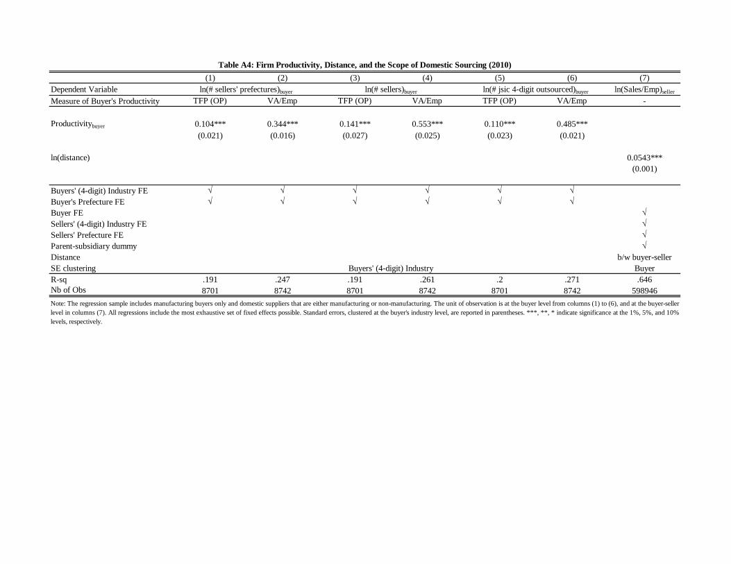
(1) (2) (3) (4) (5) (6) (7)Dependent Variable ln(Sales/Emp)seller
Measure of Buyer's Productivity TFP (OP) VA/Emp TFP (OP) VA/Emp TFP (OP) VA/Emp -
Productivitybuyer 0.104*** 0.344*** 0.141*** 0.553*** 0.110*** 0.485***(0.021) (0.016) (0.027) (0.025) (0.023) (0.021)
ln(distance) 0.0543***(0.001)
Buyers' (4-digit) Industry FE √ √ √ √ √ √Buyer's Prefecture FE √ √ √ √ √ √Buyer FE √Sellers' (4-digit) Industry FE √Sellers' Prefecture FE √Parent-subsidiary dummy √Distance b/w buyer-sellerSE clustering BuyerR-sq .191 .247 .191 .261 .2 .271 .646Nb of Obs 8701 8742 8701 8742 8701 8742 598946
Buyers' (4-digit) Industry
Note: The regression sample includes manufacturing buyers only and domestic suppliers that are either manufacturing or non-manufacturing. The unit of observation is at the buyer level from columns (1) to (6), and at the buyer-sellerlevel in columns (7). All regressions include the most exhaustive set of fixed effects possible. Standard errors, clustered at the buyer's industry level, are reported in parentheses. ***, **, * indicate significance at the 1%, 5%, and 10%levels, respectively.
Table A4: Firm Productivity, Distance, and the Scope of Domestic Sourcing (2010)
ln(# sellers' prefectures)buyer ln(# sellers)buyer ln(# jsic 4-digit outsourced)buyer
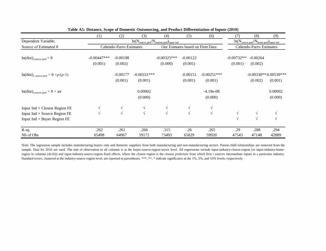
(1) (2) (3) (4) (5) (6) (7) (8) (9)Dependent Variable:Source of Estimated θ
ln(dist)i,source pref × θ -0.00447*** -0.00198 -0.00325*** -0.00122 -0.00732*** -0.00264(0.001) (0.002) (0.000) (0.001) (0.001) (0.002)
ln(dist)i, source pref × θ ×ρ/(ρ-1) -0.00177 -0.00331*** -0.00151 -0.00251*** -0.00330**-0.00539***(0.001) (0.001) (0.001) (0.001) (0.002) (0.001)
ln(dist)i,source pref × θ × air 0.00002 -4.19e-08 0.00002(0.000) (0.000) (0.000)
Input Ind × Closest Region FE √ √ √ √ √ √Input Ind × Source Region FE √ √ √ √ √ √ √ √ √Input Ind × Buyer Region FE √ √ √
R-sq .262 .261 .266 .315 .26 .265 .29 .288 .294Nb of Obs 65498 64967 59172 73493 65829 59920 47543 47148 42889
Note: The regression sample includes manufacturing buyers only and domestic suppliers from both manufacturing and non-manufacturing sectors. Parent-child relationships are removed from thesample. Data for 2010 are used. The unit of observation in all columns is at the buyer-source-region-sector level. All regressions include input-industry-closest-region (or input-industry-home-region in columns (4)-(6)) and input-industry-source-region fixed effects, where the closest region is the closest prefecture from which firm i sources intermediate inputs in a particular industry.Standard errors, clustered at the industry-source-region level, are reported in parentheses. ***, **, * indicate significance at the 1%, 5%, and 10% levels, respectively.
Table A5: Distance, Scope of Domestic Outsourcing, and Product Differentiation of Inputs (2010)
ln(Nsource pref/Nnearest pref)input ind ln(Nsource pref/Nhome pref)input ind
Caliendo-Parro Estimates Our Esimates based on Firm Data Caliendo-Parro Estimates
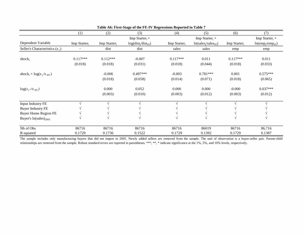
(1) (2) (3) (4) (5) (6) (7)
Dependent Variable Imp Starteri Imp Starteri
Imp Starteri × log(distj/dist05) Imp Starteri
Imp Starteri × ln(salesj/sales05) Imp Starteri
Imp Starteri × ln(empj/emp05)
Seller's Characteristics (x j ) - dist dist sales sales emp emp
shocki 0.117*** 0.112*** -0.007 0.117*** 0.011 0.117*** 0.011(0.018) (0.018) (0.031) (0.018) (0.044) (0.018) (0.033)
shocki × log(x j /x i05 ) -0.006 0.497*** -0.003 0.781*** 0.001 0.575***(0.018) (0.058) (0.014) (0.071) (0.018) (0.065)
log(x j -/x i05 ) 0.000 0.052 0.000 0.000 -0.000 0.037***(0.003) (0.010) (0.003) (0.012) (0.003) (0.012)
Input Industry FE √ √ √ √ √ √ √Buyer Industry FE √ √ √ √ √ √ √Buyer Home Region FE √ √ √ √ √ √ √Buyer's ln(sales)2005 √ √ √ √ √ √ √
Nb of Obs 86716 86716 86716 86716 86019 86716 86,716R-squared 0.1729 0.1736 0.1522 0.1729 0.1392 0.1729 0.1387
Table A6: First-Stage of the FE-IV Regressions Reported in Table 7
The sample includes only manufacturing buyers that did not import in 2005. Newly added sellers are removed from the sample. The unit of observation is a buyer-seller pair. Parent-childrelationships are removed from the sample. Robust standard errors are reported in parentheses. ***, **, * indicate significance at the 1%, 5%, and 10% levels, respectively.
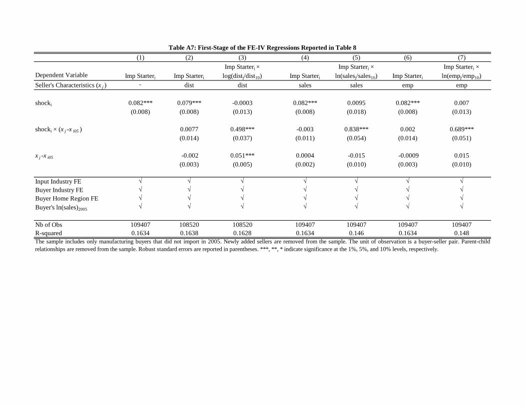
(1) (2) (3) (4) (5) (6) (7)
Dependent Variable Imp Starteri Imp Starteri
Imp Starteri × log(distj/dist10) Imp Starteri
Imp Starteri × ln(salesj/sales10) Imp Starteri
Imp Starteri × ln(empj/emp10)
Seller's Characteristics (x j ) - dist dist sales sales emp emp
shocki 0.082*** 0.079*** -0.0003 0.082*** 0.0095 0.082*** 0.007(0.008) (0.008) (0.013) (0.008) (0.018) (0.008) (0.013)
shocki × (x j -x i05 ) 0.0077 0.498*** -0.003 0.838*** 0.002 0.689***(0.014) (0.037) (0.011) (0.054) (0.014) (0.051)
x j -x i05 -0.002 0.051*** 0.0004 -0.015 -0.0009 0.015(0.003) (0.005) (0.002) (0.010) (0.003) (0.010)
Input Industry FE √ √ √ √ √ √ √Buyer Industry FE √ √ √ √ √ √ √Buyer Home Region FE √ √ √ √ √ √ √Buyer's ln(sales)2005 √ √ √ √ √ √ √
Nb of Obs 109407 108520 108520 109407 109407 109407 109407R-squared 0.1634 0.1638 0.1628 0.1634 0.146 0.1634 0.148
Table A7: First-Stage of the FE-IV Regressions Reported in Table 8
The sample includes only manufacturing buyers that did not import in 2005. Newly added sellers are removed from the sample. The unit of observation is a buyer-seller pair. Parent-childrelationships are removed from the sample. Robust standard errors are reported in parentheses. ***, **, * indicate significance at the 1%, 5%, and 10% levels, respectively.
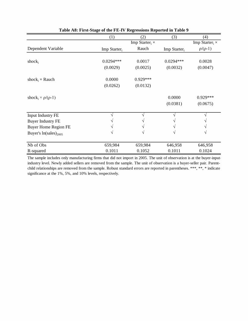
(1) (2) (3) (4)
Dependent Variable Imp Starteri
Imp Starteri × Rauch Imp Starteri
Imp Starteri × ρ/(ρ-1)
shocki 0.0294*** 0.0017 0.0294*** 0.0028(0.0029) (0.0025) (0.0032) (0.0047)
shocki × Rauch 0.0000 0.929***(0.0262) (0.0132)
shocki × ρ/(ρ-1) 0.0000 0.929***(0.0381) (0.0675)
Input Industry FE √ √ √ √Buyer Industry FE √ √ √ √Buyer Home Region FE √ √ √ √Buyer's ln(sales)2005 √ √ √ √
Nb of Obs 659,984 659,984 646,958 646,958R-squared 0.1011 0.1052 0.1011 0.1024
Table A8: First-Stage of the FE-IV Regressions Reported in Table 9
The sample includes only manufacturing firms that did not import in 2005. The unit of observation is at the buyer-input-industry level. Newly added sellers are removed from the sample. The unit of observation is a buyer-seller pair. Parent-child relationships are removed from the sample. Robust standard errors are reported in parentheses. ***, **, * indicate significance at the 1%, 5%, and 10% levels, respectively.
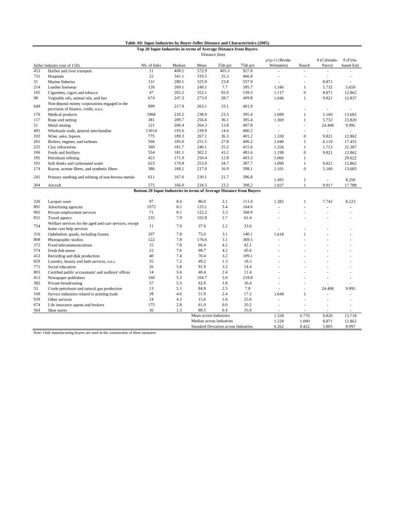
Nb. of links Median Mean 25th pct 75th pctρ/(ρ-1) (Broda-
Weinstein) Rauchθ (Caliendo-
Parro)θ (Firm-
based Est)453 Harbor and river transport 11 408.1 572.9 405.5 927.8 - - - -731 Hospitals 22 341.1 319.5 25.3 466.8 - - - -31 Marine fisheries 131 280.1 325.9 23.8 557.9 - - 8.871 -214 Leather footwear 126 269.1 249.1 7.7 395.7 1.186 1 5.732 5.659105 Cigarettes, cigars and tobacco 47 265.2 352.1 92.0 539.3 1.117 0 8.871 12.86298 Vegitable oils, animal oils, and fats 674 247.3 273.9 28.7 409.8 1.046 1 9.821 12.837
649 Non-deposit money corporations engaged in the provision of finance, credit, n.e.c. 899 217.9 263.1 33.1 401.9
- - - -176 Medical products 1866 210.2 238.9 23.3 395.4 1.089 1 5.160 13.683117 Rope and netting 381 209.7 256.6 36.1 395.4 1.369 1 5.732 23.82051 Metal mining 121 206.4 264.3 13.8 407.8 - - 24.498 9.995491 Wholesale trade, general merchandise 13014 193.6 239.9 14.6 400.2 - - - -102 Wine, sake, liquors 775 189.3 267.1 36.3 401.2 1.330 0 9.821 12.862261 Boilers, engines, and turbines 566 185.0 251.5 27.8 406.2 1.040 1 6.119 17.455225 Clay refractories 360 181.7 246.1 25.2 415.6 1.326 1 1.713 22.387106 Feeds and fertiliers 554 181.1 302.2 43.2 481.6 1.198 0 9.821 12.862181 Petroleum refining 423 171.9 250.4 12.8 403.3 1.060 1 29.622101 Soft drinks and carbonated water 623 170.8 253.9 34.7 387.7 1.090 1 9.821 12.862174 Rayon, acetate fibers, and synthetic fibers 386 168.1 217.0 16.9 398.1 1.101 0 5.160 13.683
241 Primary smelting and refining of non-ferrous metals 611 167.6 230.1 21.7 396.81.495 1 - 8.250
304 Aircraft 575 166.0 234.5 23.2 398.2 1.027 1 9.917 17.788
326 Lacquer ware 97 8.4 86.0 2.1 111.0 1.382 1 7.742 8.223891 Advertising agencies 1972 8.2 125.1 3.4 164.0 - - - -905 Private employment services 71 8.1 122.2 3.3 368.9 - - - -831 Travel agency 235 7.9 102.8 2.7 61.4 - - - -
754 Welfare services for the aged and care services, except home care help services 11 7.9 37.6 2.2 33.6
- - - -316 Ophthalmic goods, including frames 207 7.8 75.0 3.1 140.1 1.618 1 - -808 Photographic studios 122 7.8 176.6 3.1 369.5 - - - -372 Fixed telecommunications 15 7.8 66.4 4.2 42.1 - - - -574 Fresh fish stores 22 7.6 98.7 4.2 45.0 - - - -412 Recording and disk production 40 7.4 70.4 3.2 109.1 - - - -829 Laundry, beauty and bath services, n.e.c. 35 7.2 49.2 1.3 18.3 - - - -771 Social education 26 5.8 91.9 3.5 14.4 - - - -803 Certified public accountants' and auditors' offices 14 5.6 40.4 2.4 11.4 - - - -413 Newspaper publishers 160 5.3 104.7 3.0 218.8 - - - -382 Private broadcasting 57 5.3 62.0 1.8 16.4 - - - -53 Crude petroleum and natural gas production 13 5.1 84.9 2.5 7.8 - - 24.498 9.995169 Service industries related to printing trade 28 4.6 51.9 2.4 17.2 1.648 1 - -939 Other services 24 4.3 15.6 1.6 25.6 - - - -674 Life insurance agents and brokers 175 2.8 61.0 0.0 20.2 - - - -564 Shoe stores 36 1.3 88.5 0.4 35.9 - - - -
1.328 0.770 9.820 13.7181.228 1.000 8.871 12.8620.262 0.422 5.805 8.997
Note: Only manufacturing buyers are used in the construction of these measures
Table A9: Input Industries by Buyer-Seller Distance and Characteristics (2005)
Distance (km)
Mean across Industries
Standard Deviation across IndustriesMedian across Industries
Seller Industry (out of 150)
Top 20 Input Industries in terms of Average Distance from Buyers
Bottom 20 Input Industries in terms of Average Distance from Buyers
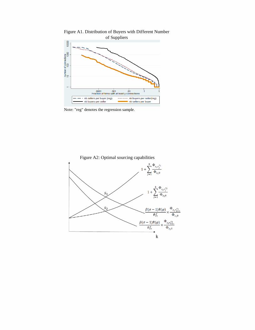
Note: "reg" denotes the regression sample.
Figure A2: Optimal sourcing capabilities
Figure A1. Distribution of Buyers with Different Number of Suppliers
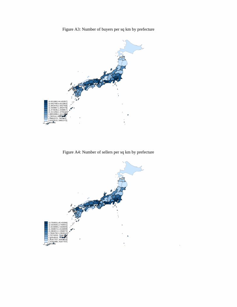
Figure A3: Number of buyers per sq km by prefecture
Figure A4: Number of sellers per sq km by prefecture
(4.621862,44.45287](2.642768,4.621862](1.892478,2.642768](1.549867,1.892478](1.475636,1.549867](1.011458,1.475636](.8853088,1.011458](.782514,.8853088](.5962272,.782514][.4202515,.5962272]No data
(3.759551,45.43396](2.333565,3.759551](1.616899,2.333565](1.358872,1.616899](1.084011,1.358872](.7846792,1.084011](.7073203,.7846792](.6054816,.7073203](.4167707,.6054816][.3192388,.4167707]No data