Global Supervised Descent Method

Xuehan Xiong and Fernando De la TorreCarnegie Mellon University, Pittsburgh PA

{xxiong,ftorre}@andrew.cmu.edu

Abstract

Mathematical optimization plays a fundamental role insolving many problems in computer vision (e.g., cameracalibration, image alignment, structure from motion). It isgenerally accepted that second order descent methods arethe most robust, fast, and reliable approaches for nonlinearoptimization of a general smooth function. However, in thecontext of computer vision, second order descent methodshave two main drawbacks: 1) the function might not be an-alytically differentiable and numerical approximations areimpractical, and 2) the Hessian may be large and not posi-tive definite. Recently, Supervised Descent Method (SDM),a method that learns the “weighted averaged gradients” ina supervised manner has been proposed to solve these is-sues. However, SDM is a local algorithm and it is likelyto average conflicting gradient directions. This paper pro-poses Global SDM (GSDM), an extension of SDM that di-vides the search space into regions of similar gradient direc-tions. GSDM provides a better and more efficient strategyto minimize non-linear least squares functions in computervision problems. We illustrate the effectiveness of GSDMin two problems: non-rigid image alignment and extrinsiccamera calibration.

1. IntroductionMany computer vision problems (e.g., camera calibra-

tion, image alignment, structure from motion) are solvedwith nonlinear optimization methods. In general, mostcomputer vision-related optimization problems of inter-est have multiple local minima and are NP-hard to solve.Global optimization algorithms are typically very computa-tionally expensive, have poor convergence properties, andgenerally suitable for low dimensional search spaces. Asa compromise, local optimization methods are usually em-ployed to find a local minimum. Whether global optimiza-tion can be solved in polynomial time is still unknown.However, there is a large number of existing techniques thatapproximate the solution. These techniques include Sim-ulated Annealing [15, 31], Evolutionary algorithms [18],

x21

x20

x11

x10

x∗f(x) = h(x)− y 2

a)

f(x) = h(x)− y 2

x1

x3x2

b)

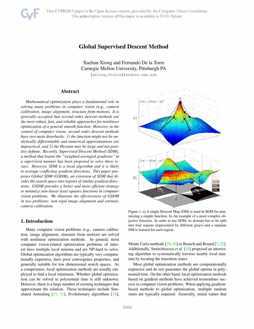
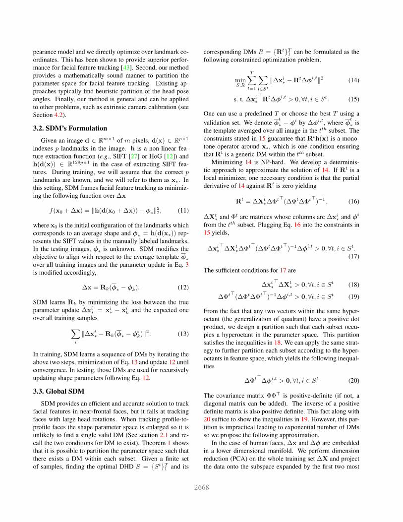
Figure 1. a) A single Descent Map (DM) is used in SDM for min-imizing a simple function. b) An example of a more complex ob-jective function. In order to use SDM, its domain has to be splitinto four regions (represented by different grays) and a separateDM is learned for each region.

Monte Carlo methods [29, 30] or Branch and Bound [7, 22].Additionally, Sminchisescu et al. [39] proposed an interest-ing algorithm to systematically traverse nearby local min-ima by locating the transition states.

Most global optimization methods are computationallyexpensive and do not guarantee the global optima in poly-nomial time. On the other hand, local optimization methodsbased on gradient methods have achieved tremendous suc-cess in computer vision problems. When applying gradient-based methods to global optimization, multiple randomstarts are typically required. Generally, initial values that

1

are close to each other give descent paths that tend to thesame minimum point. This phenomenon is formally knownas basin of attraction, the set of initial values leading to thesame local minimum. In the context of local optimization,it is generally accepted that for a general smooth function,second order descent methods are the most robust, fast, andreliable approaches for nonlinear optimization. However,in the context of computer vision, second order descentmethods have two main drawbacks: 1) the function mightnot be analytically differentiable and numerical approxima-tions are impractical, and 2) the Hessian may be large andnot positive definite. To address these issues, Xiong andDe la Torre [44] proposed a Supervised Descent Method(SDM) for optimizing Nonlinear Least Squares (NLS) func-tions. Unlike previous methods, it uses supervised data todrive the optimization search. SDM has shown promisingresults in face alignment [1, 25, 43, 46, 48] and been ex-tended to other computer vision applications such as, objectpose estimation [44], rigid object tracking [44], object re-localization [26], human pose estimation [45], and objectpart localization [45].

Fig. 1a illustrates the idea of SDM. During training, ineach iteration SDM learns a single generic Descent Map(DM) from the optimal optimization trajectories (indicatedby the dotted lines). In testing, the same DM is used fordriving an unseen sample to x∗ (the labeled ground-truth).DM exists under two mild conditions (see Section 2.1). Forsimple functions, such conditions normally hold. However,in many real applications the function might have several lo-cal minima in a relatively small neighborhood, for instancesee Fig. 1b for an example. Standard SDM would averageconflicting gradient directions resulting in undesirable per-formance. To overcome this issue, GSDM learns not onebut a set of generic DMs (in this example, four), one fordifferent domains (colored by different intensity of grays) ofthe objective function. Each domain contains only similargradient directions and one separate DM is learned for each.At iteration k, xk may step into any of the four regions andthe corresponding DM is used to update the result. Basedon this intuition, this paper introduces and validates a newconcept, domain of homogeneous descent and extends thetheory of SDM to global optimization. In addition, we dis-cover the connection between SDM and Imitation Learningand develop a practical algorithm based on GSDM to trackfaces from profile to profile and illustrate how GSDM canalso be used for extrinsic camera calibration.

2. TheoryIn this section, we extend the theory of SDM to deal

with multiple local minima. First, we review the conceptof DM and the two conditions for it to exist. Second, wediscuss SDM’s interesting connection with Imitation Learn-ing. Then, we introduce and validate a new concept termed,

domains of homogeneous descent.

2.1. Review of SDM

This section reviews SDM originally introduced in [44]and its theoretical properties. See footnote1 for notation.Given a Nonlinear Least Squares (NLS) problem,

minxf(x) = min

x‖h(x)− y‖2, (1)

where h(x) : Rn → Rm is a nonlinear function, y ∈ Rm

is a known vector, and x ∈ Rn is the optimizing parameter.Applying the chain rule to Eq. 1, the gradient descent updaterule yields

xk = xk−1 − αAJ>h (xk−1)(h(xk−1)− y) (2)

where Jh(x) ∈ Rm×n is the Jacobian matrix, A ∈ Rn×n isthe identity (In) in first-order methods, or the inverse Hes-sian (or an approximation) for second-order methods, and αis the step size. Computing the rescaling factor A and gradi-ent direction Jh in high-dimensional spaces is computation-ally expensive and can be numerically unstable, especiallyin the case of non-differentiable functions, where finite dif-ferences are required to compute estimates of the Hessianand Jacobian. The main idea behind SDM is to avoid ex-plicit computation of the Hessian and Jacobian and learnthe generic DM (R ∼ αAJh(xk−1)) from training data.Note that DM is not a descent direction, it contains part ofdescent direction and needs to multiply with (h(x)− y) toproduce a descent direction. Alternatively, R can be seen asthe “weighted average gradient direction” of h around x∗.We define R more formally below.

Definition 1. A matrix R ∈ Rn×m is called a generic de-scent map if there exists a scalar 0 < c < 1 such that∀x ∈ N(x∗), ‖x∗ − xk‖ ≤ c‖x∗ − xk−1‖. xk is updatedusing the following equation:

xk = xk−1 −R(h(xk−1)− h(x∗)). (3)

Xiong and De la Torre [44] proved the existence of ageneric DM under the following conditions: 1). Rh(x) isa strictly locally monotone operator anchored at the opti-mal solution x∗. 2). h(x) is locally Lipschitz continuousanchored at x∗.

2.2. SDM as Policy Learning

Imitation Learning (IL) can be seen as a special case ofSupervised Learning. In Supervised Learning, the agent is

1 Bold capital letters denote a matrix X; bold lower-case letters denotea column vector x. All non-bold letters represent scalars. xi representsthe ith column of the matrix X. xij denotes the scalar in the ith row andjth column of the matrix X. xj denotes the scalar in the jth elementof x. In ∈ Rn×n is an identity matrix. ‖x‖ =

√xTx denotes the

Euclidean distance. ‖X‖F =√

tr(XTX) =√

tr(XXT ) designatesthe Frobenious norm of a matrix. N(x) denotes the neighborhood of x.

presented with labeled training data and learns an approx-imation to the function that produced the data. Within IL,this training dataset is composed of example executions (se-quences of state and action pairs) of the task by a demon-stration teacher. The goal is to derive a policy that repro-duces the demonstrated behavior. The world consists ofstates S, actionsA, and a policy is the mapping between thetwo. In real-world applications, the state is often not fullyobservable and the learner instead has access to an observedstate Z.

In the context of minimizing a NLS function, y is re-garded as the desired state and the objective is to find theaction ∆x that moves from the initial state to the desiredstate. The nonlinear function h is the feature function thatpartially represents the state. The demonstration data con-tains a set of observation and action pairs. The observedstates are represented by a set Z = {h(xi) − yi} of er-rors (misalignments) between the known vectors {yi} andthe function evaluations at the current parameter estimates{h(xi)}. The action set will correspond to the parameterupdates A = {∆xi}, and the policy maps misalignmentsto parameter updates. In SDM, the policy is derived as asequence of linear mapping functions between states andactions. Within this context, the teacher is always availablefor giving feedback. More specifically, since the groundtruth solutions {xi

∗} are available throughout training, theteacher can always give the perfect action based on the stateobservation. SDM takes advantage of this fact by learningnot one but a sequence of policies so the latter ones correctmistakes made from previous iterations after the teacher’sfeedbacks.

2.3. Domains of Homogeneous Descent

For a function f with a unique minimum, the gradientsof h often share similar directions. Therefore, a weightedaverage can be learned. When dealing with the function fwith several local minima (See Fig. 1b for an example), thegradients of h may have conflicting directions so averagingthem is not adequate and it may cause the SDM training tostall. Later in the paper, we validate this intuition in ourexperiments on extrinsic camera calibration. When we en-large the parameter space, the performance of SDM dropsdramatically.

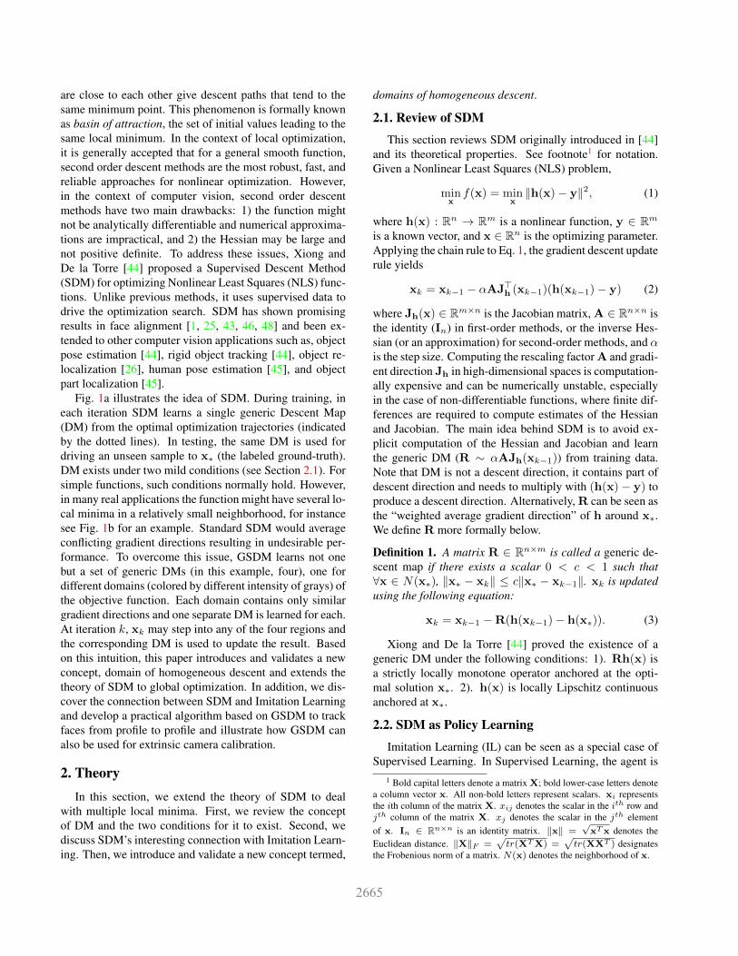
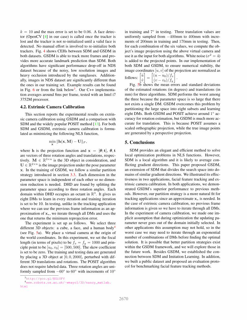
We will bypass this problem by learning not one but aset of DMs. In the following, we will prove that it is pos-sible to find a partition of domain x, S = {St}T1 , such thatthere exists a generic DM Rt,∀t,x ∈ St. The subsets ofthis partition is defined as Domains of Homogeneous De-scent (DHD). In Fig. 2 we plot four NLS functions alongwith their DHD found by following the strategy proposedin Theorem 1. Interestingly, local minima are located at theintersections of different domains.

Theorem 1. Under one minor condition:

∃K > 0,‖h(x)− h(x∗)‖‖x− x∗‖

< K,∀x ∈ N(x∗), (4)

there exists a finite partition of domain x, S = {St}T1 , suchthat ∀x ∈ St, there exists a generic DM Rt.

Proof. To simplify the notation, we denote x∗ − x as ∆xand h(x∗) − h(x) as ∆h. We will prove the above the-orem by finding a specific partition with its correspondingDMs. Let us consider a partition strategy based on the signsof ∆xj∆hj . Each sign can take on two values ±1 and jranges from 1 to min(n,m). Each subset of this partitioncontains x that satisfy one of the 2min(n,m) unique condi-tions. Without loss of generality, let us derive the DM forthe subset S0 where ∀j, sign(∆xj∆hj) = 1. We want toshow that there exists a R such that

‖x∗ − xik‖

‖x∗ − xik−1‖

< 1, if x∗ 6= xik−1. (5)

We replace xik with xi

k−1 using Eq. 3 and squaring the leftside of Eq. 5 gives us,

‖∆xik‖2

‖∆xik−1‖2

=‖∆xi

k−1 −R∆hik−1‖2

‖∆xik−1‖2

=‖∆xi

k−1‖2‖∆xi

k−1‖2+‖R∆hi

k−1‖2‖∆xi

k−1‖2− 2

∆xi>

k−1R∆hik−1

‖∆xik−1‖2

=1 +‖R∆hi

k−1‖‖∆xi

k−1‖2(‖R∆hi

k−1‖ − 2∆xi>

k−1R∆hi

k−1‖R∆hi

k−1‖

).

(6)

Setting Eq. 6 < 1 gives us,

‖R∆hik−1‖ ≤ 2∆xi>

k−1R∆hi

k−1‖R∆hi

k−1‖. (7)

The choice of R needs to guarantee that the right side ofEq. 7 is greater than zero. Remember that in subset S(0)

sign(∆xj∆hj) = 1,∀j. A trivial R would be cD, wherec > 0 and D is a rectangular diagonal matrix with the diag-onal elements equal to 1. From the geometric definition ofdot product, we can rewrite the right side of the inequality 7as,

2∆xi>

k−1R∆hi

k−1‖R∆hi

k−1‖= 2‖∆xi

k−1‖ cos θi,

where θi is the angle between vectors ∆xik−1 and

R∆hik−1. Using the condition stated in 4 we have

2‖∆xik−1‖ cos θi ≥ 2

K‖∆hi

k−1‖ cos θi. (8)

From the Cauchy-Schwartz inequality,

‖R∆hik−1‖ ≤ ‖R‖F ‖∆hi

k−1‖. (9)

f(x) = h(x)− y 2 f(x) = h(x)− y 2

f(x) = h(x)− y 2f(x) = h(x)− y 2

(d)(c)

(a) (b)

Figure 2. Illustration of DHD on four NLS functions where h(x) :R2 → R2. Different domains are colored in different grayscales.

Given the inequalities in Eqs. 8 and 9, the condition thatmakes Eq. 7 hold is,

‖R‖F =√c‖D‖F =

√c ≤ 2

Kcos θi. (10)

Any R = cD where√c < 2

K mini cos θi guarantees theinequality stated in Eq. 5. Therefore, there exists a genericDM for subset S(0). For other subsets in the partition ageneral choice of D has the entries

dij =

{0 if i 6= jsign(∆xij,k−1∆hij,k−1) Otherwise.

Following the same proof we can easily show DM exist forother subsets in the partition.

Above, we proposed a simple partition strategy andproved the existence of DHD. In the next section, basedon this strategy we derive a practical algorithm with ap-plications to extrinsic camera calibration and facial featuretracking.

3. Application to Facial Feature Tracking

In this section we first review previous work on track-ing profile-to-profile faces and the SDM’s formulation onthis problem. Next, we derive a simple strategy for findingDHD of the tracking objective function and following thisstrategy we extend SDM to track profile-to-profile faces.

3.1. Previous Work on Multi-view Face Tracking

Previous work on multi-view facial feature tracking canbe grouped into two categories based on whether a 2D or3D face model is used.

Let us first review some of the 2D model based ap-proaches. The shape of a deformable object can be mod-eled by a probability density function. A multi-modal 2Dface model can be represented either in a non-parametricway e.g., kernel density estimation [38] or in a paramet-ric way, e.g., a mixture of Gaussians [8]. Therefore, thereare two common strategies to extend traditional frontal facealignment methods to multi-view tracking. The first one isto build separate models according to the head pose. Someof the examples are multi-view Active Appearance Model(AAM) [10], view-based Active Wavelet Networks [19],and multi-view Direct Appearance Models [24]. The otheris to use kernel methods. For example, Romdhani et al. [33]extended Active Shape Model [9] to track profile-to-profilefaces. They used kernel PCA [36] to non-linearly modelthe shape variation across large pose changes. However,kernel-based density estimation is slow and its complexityincreases with number of training samples. Another inter-esting work [47] treated the shape parameter and pose ashidden variables and framed the alignment problem into aBayesian framework. However, the inference is intractableso the EM algorithm (local minima prone) is used to ap-proximate the solution. Beyond the two common strategies,another way to address the multi-view problem would beonline tracking. Ellis et al. [14] proposed an efficient onlinetracker using adaptive appearance models, and one couldextend this approach to track faces and other nonrigid ob-jects.

Next, let us take a look at 3D model based approaches.Matthews et al. [28] provided a detailed comparison be-tween 2D and 3D face models in three different aspects, fit-ting speed, representational power, and construction. Theyconcluded that 2D face model may be too “powerful” thatcan represent invalid faces. Xiao et al. [42] extended theAAM fitting algorithm to impose additional shape con-straints introduced by a 3D model that are lacked in the 2Dmodel. Baltrusaitis et al. [2] extended Constrained LocalModels [11] for RGBD data streams and show better align-ment performance than its original. However, the trainingdata is difficult to collect. Gu and Kanade [17] formulatedmulti-view face alignment as a Bayesian inference problemwith missing data, whose task is to solve 3D shape and 3Dpose from the noisy and incomplete 2D shape observation.Recently, Cao et al. [5] extended an earlier 2D regression-based framework [6] with a 3D face model, but only near-frontal face results are shown in the experiments. Other in-teresting work [37, 40, 49] have been proposed for detect-ing facial landmarks in the profile-to-profile faces but theyare not suitable for tracking applications. Note that most3D based methods still rely on head pose to build separatemodels to address the multi-view problem.

Our work differs from existing approaches in severalways. First, our approach do not pre-build any shape or ap-

pearance model and we directly optimize over landmark co-ordinates. This has been shown to provide superior perfor-mance for facial feature tracking [43]. Second, our methodprovides a mathematically sound manner to partition theparameter space for facial feature tracking. Existing ap-proaches typically find heuristic partition of the head poseangles. Finally, our method is general and can be appliedto other problems, such as extrinsic camera calibration (seeSection 4.2).

3.2. SDM’s Formulation

Given an image d ∈ Rm×1 of m pixels, d(x) ∈ Rp×1

indexes p landmarks in the image. h is a non-linear fea-ture extraction function (e.g., SIFT [27] or HoG [12]) andh(d(x)) ∈ R128p×1 in the case of extracting SIFT fea-tures. During training, we will assume that the correct plandmarks are known, and we will refer to them as x∗. Inthis setting, SDM frames facial feature tracking as minimiz-ing the following function over ∆x

f(x0 + ∆x) = ‖h(d(x0 + ∆x))− φ∗‖22, (11)

where x0 is the initial configuration of the landmarks whichcorresponds to an average shape and φ∗ = h(d(x∗)) rep-resents the SIFT values in the manually labeled landmarks.In the testing images, φ∗ is unknown. SDM modifies theobjective to align with respect to the average template φ∗over all training images and the parameter update in Eq. 3is modified accordingly,

∆x = Rk(φ∗ − φk). (12)

SDM learns Rk by minimizing the loss between the trueparameter update ∆xi

∗ = xi∗ − xi

k and the expected oneover all training samples∑

i

‖∆xi∗ −Rk(φ∗ − φi

k)‖2. (13)

In training, SDM learns a sequence of DMs by iterating theabove two steps, minimization of Eq. 13 and update 12 untilconvergence. In testing, those DMs are used for recursivelyupdating shape parameters following Eq. 12.

3.3. Global SDM

SDM provides an efficient and accurate solution to trackfacial features in near-frontal faces, but it fails at trackingfaces with large head rotations. When tracking profile-to-profile faces the shape parameter space is enlarged so it isunlikely to find a single valid DM (See section 2.1 and re-call the two conditions for DM to exist). Theorem 1 showsthat it is possible to partition the parameter space such thatthere exists a DM within each subset. Given a finite setof samples, finding the optimal DHD S = {St}T1 and its

corresponding DMs R = {Rt}T1 can be formulated as thefollowing constrained optimization problem,

minS,R

T∑t=1

∑i∈St

‖∆xi∗ −Rt∆φi,t‖2 (14)

s. t. ∆xi∗>Rt∆φi,t > 0,∀t, i ∈ St. (15)

One can use a predefined T or choose the best T using avalidation set. We denote φ

t

∗ − φi by ∆φi,t, where φt

∗ isthe template averaged over all image in the tth subset. Theconstraints stated in 15 guarantee that Rth(x) is a mono-tone operator around x∗, which is one condition ensuringthat Rt is a generic DM within the tth subset.

Minimizing 14 is NP-hard. We develop a determinis-tic approach to approximate the solution of 14. If Rt is alocal minimizer, one necessary condition is that the partialderivative of 14 against Rt is zero yielding

Rt = ∆Xt∗∆Φt>(∆Φt∆Φt>)−1. (16)

∆Xt∗ and Φt are matrices whose columns are ∆xi

∗ and φi

from the tth subset. Plugging Eq. 16 into the constraints in15 yields,

∆xi∗>

∆Xt∗∆Φt>(∆Φt∆Φt>)−1∆φi,t > 0,∀t, i ∈ St.

(17)

The sufficient conditions for 17 are

∆xi∗>

∆Xt∗ > 0,∀t, i ∈ St (18)

∆Φt>(∆Φt∆Φt>)−1∆φi,t > 0,∀t, i ∈ St (19)

From the fact that any two vectors within the same hyper-octant (the generalization of quadrant) have a positive dotproduct, we design a partition such that each subset occu-pies a hyperoctant in the parameter space. This partitionsatisfies the inequalities in 18. We can apply the same strat-egy to further partition each subset according to the hyper-octants in feature space, which yields the following inequal-ities

∆Φt>∆φi,t > 0,∀t, i ∈ St (20)

The covariance matrix ΦΦ> is positive-definite (if not, adiagonal matrix can be added). The inverse of a positivedefinite matrix is also positive definite. This fact along with20 suffice to show the inequalities in 19. However, this par-tition is impractical leading to exponential number of DMsso we propose the following approximation.

In the case of human faces, ∆x and ∆φ are embeddedin a lower dimensional manifold. We perform dimensionreduction (PCA) on the whole training set ∆X and projectthe data onto the subspace expanded by the first two most

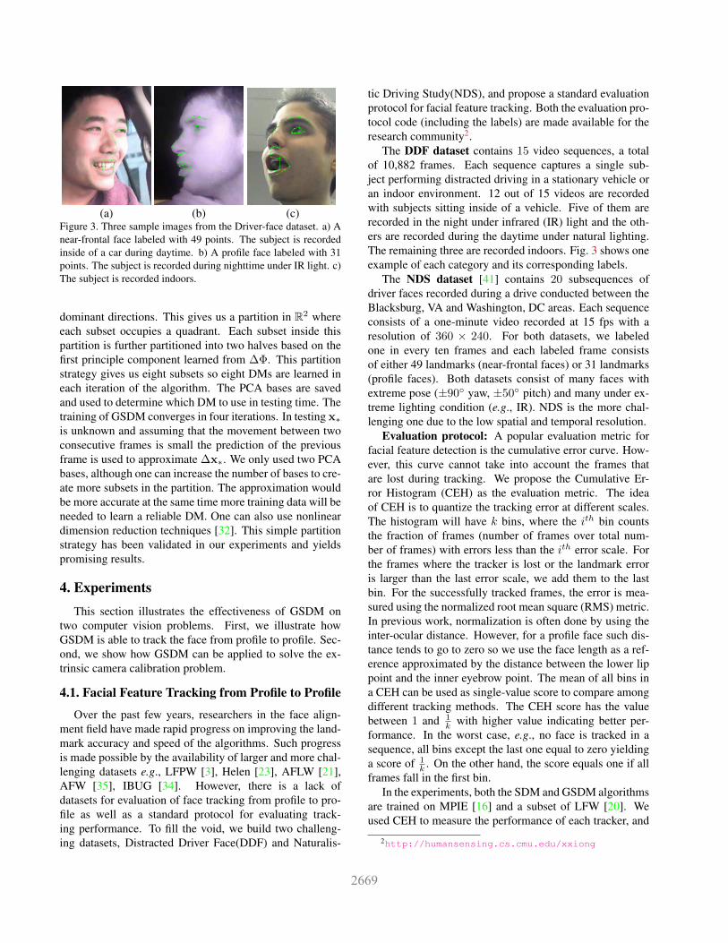
(a) (b) (c)Figure 3. Three sample images from the Driver-face dataset. a) Anear-frontal face labeled with 49 points. The subject is recordedinside of a car during daytime. b) A profile face labeled with 31points. The subject is recorded during nighttime under IR light. c)The subject is recorded indoors.

dominant directions. This gives us a partition in R2 whereeach subset occupies a quadrant. Each subset inside thispartition is further partitioned into two halves based on thefirst principle component learned from ∆Φ. This partitionstrategy gives us eight subsets so eight DMs are learned ineach iteration of the algorithm. The PCA bases are savedand used to determine which DM to use in testing time. Thetraining of GSDM converges in four iterations. In testing x∗is unknown and assuming that the movement between twoconsecutive frames is small the prediction of the previousframe is used to approximate ∆x∗. We only used two PCAbases, although one can increase the number of bases to cre-ate more subsets in the partition. The approximation wouldbe more accurate at the same time more training data will beneeded to learn a reliable DM. One can also use nonlineardimension reduction techniques [32]. This simple partitionstrategy has been validated in our experiments and yieldspromising results.

4. ExperimentsThis section illustrates the effectiveness of GSDM on

two computer vision problems. First, we illustrate howGSDM is able to track the face from profile to profile. Sec-ond, we show how GSDM can be applied to solve the ex-trinsic camera calibration problem.

4.1. Facial Feature Tracking from Profile to Profile

Over the past few years, researchers in the face align-ment field have made rapid progress on improving the land-mark accuracy and speed of the algorithms. Such progressis made possible by the availability of larger and more chal-lenging datasets e.g., LFPW [3], Helen [23], AFLW [21],AFW [35], IBUG [34]. However, there is a lack ofdatasets for evaluation of face tracking from profile to pro-file as well as a standard protocol for evaluating track-ing performance. To fill the void, we build two challeng-ing datasets, Distracted Driver Face(DDF) and Naturalis-

tic Driving Study(NDS), and propose a standard evaluationprotocol for facial feature tracking. Both the evaluation pro-tocol code (including the labels) are made available for theresearch community2.

The DDF dataset contains 15 video sequences, a totalof 10,882 frames. Each sequence captures a single sub-ject performing distracted driving in a stationary vehicle oran indoor environment. 12 out of 15 videos are recordedwith subjects sitting inside of a vehicle. Five of them arerecorded in the night under infrared (IR) light and the oth-ers are recorded during the daytime under natural lighting.The remaining three are recorded indoors. Fig. 3 shows oneexample of each category and its corresponding labels.

The NDS dataset [41] contains 20 subsequences ofdriver faces recorded during a drive conducted between theBlacksburg, VA and Washington, DC areas. Each sequenceconsists of a one-minute video recorded at 15 fps with aresolution of 360 × 240. For both datasets, we labeledone in every ten frames and each labeled frame consistsof either 49 landmarks (near-frontal faces) or 31 landmarks(profile faces). Both datasets consist of many faces withextreme pose (±90◦ yaw, ±50◦ pitch) and many under ex-treme lighting condition (e.g., IR). NDS is the more chal-lenging one due to the low spatial and temporal resolution.

Evaluation protocol: A popular evaluation metric forfacial feature detection is the cumulative error curve. How-ever, this curve cannot take into account the frames thatare lost during tracking. We propose the Cumulative Er-ror Histogram (CEH) as the evaluation metric. The ideaof CEH is to quantize the tracking error at different scales.The histogram will have k bins, where the ith bin countsthe fraction of frames (number of frames over total num-ber of frames) with errors less than the ith error scale. Forthe frames where the tracker is lost or the landmark erroris larger than the last error scale, we add them to the lastbin. For the successfully tracked frames, the error is mea-sured using the normalized root mean square (RMS) metric.In previous work, normalization is often done by using theinter-ocular distance. However, for a profile face such dis-tance tends to go to zero so we use the face length as a ref-erence approximated by the distance between the lower lippoint and the inner eyebrow point. The mean of all bins ina CEH can be used as single-value score to compare amongdifferent tracking methods. The CEH score has the valuebetween 1 and 1

k with higher value indicating better per-formance. In the worst case, e.g., no face is tracked in asequence, all bins except the last one equal to zero yieldinga score of 1

k . On the other hand, the score equals one if allframes fall in the first bin.

In the experiments, both the SDM and GSDM algorithmsare trained on MPIE [16] and a subset of LFW [20]. Weused CEH to measure the performance of each tracker, and

2http://humansensing.cs.cmu.edu/xxiong

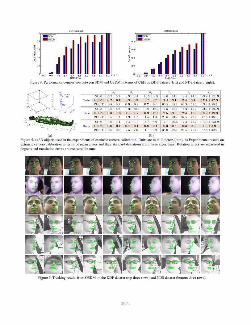
k = 10 and the max error is set to be 0.06. A face detec-tor (OpenCV [4] in our case) is called once the tracker islost and the tracker is not re-initialized until a valid face isdetected. No manual effort is involved to re-initialize bothtrackers. Fig. 4 shows CEHs between SDM and GSDM inboth datasets. GSDM is able to track more frames and pro-vides more accurate landmark prediction than SDM. Bothalgorithms have significant performance drop-off in NDSdataset because of the noisy, low resolution images andheavy occlusion introduced by the sunglasses. Addition-ally, images in NDS dataset are significantly different thanthe ones in our training set. Example results can be foundin Fig. 6 or from the link below3. Our C++ implementa-tion averages around 8ms per frame, tested with an Intel i73752M processor.

4.2. Extrinsic Camera Calibration

This section reports the experimental results on extrin-sic camera calibration using GSDM and a comparison withSDM and the widely popular POSIT method [13]. For bothSDM and GSDM, extrinsic camera calibration is formu-lated as minimizing the following NLS function,

minx‖h(x,M)−U‖F ,

where h is the projection function and x = [θ; t], θ, tare vectors of three rotation angles and translations, respec-tively. M ∈ R3×n is the 3D object in consideration, andU ∈ R2×n is the image projection under the pose parameterx. In the training of GSDM, we follow a similar partitionstrategy introduced in section 3.3. Each dimension in theparameter space is independent of each other so no dimen-sion reduction is needed. DHD are found by splitting theparameter space according to three rotation angles. Eachdomain within DHD occupies an octant in R3. It gives useight DMs to learn in every iteration and training iterationis set to be 10. In testing, unlike in the tracking applicationwhere we can use the previous frame information as an ap-proximation of x∗, we iterate through all DMs and uses theone that returns the minimum reprojection error.

The experiment is set up as follows. We select threedifferent 3D objects: a cube, a face, and a human body4

(see Fig. 5a). We place a virtual camera at the origin ofthe world coordinates. In this experiment, we set the focallength (in terms of pixels) to be fx = fy = 1000 and prin-ciple point to be [u0, v0] = [500, 500]. The skew coefficientis set to be zero. The training and testing data are generatedby placing a 3D object at [0, 0, 2000], perturbed with dif-ferent 3D translations and rotations. The POSIT algorithmdoes not require labeled data. Three rotation angles are uni-formly sampled from −60◦ to 60◦ with increments of 10◦

3http://goo.gl/EGiUFV4www.robots.ox.ac.uk/˜wmayol/3D/nancy_matlab.

html

in training and 7◦ in testing. Three translation values areuniformly sampled from −400mm to 400mm with incre-ments of 200mm in training and 170mm in testing. Then,for each combination of the six values, we compute the ob-ject’s image projection using the above virtual camera anduse it as the input for both algorithms. White noise (σ2 = 4)is added to the projected points. In our implementation ofboth SDM and GSDM, to ensure numerical stability, theimage coordinates [u, v] of the projection are normalized as

follows:[uv

]=

[(u− u0)/fx(v − v0)/fy

].

Fig. 5b shows the mean errors and standard deviationsof the estimated rotations (in degrees) and translations (inmm) for three algorithms. SDM performs the worst amongthe three because the parameter space is so large that therenot exists a single DM. GSDM overcomes this problem bypartitioning the large space into eight subsets and learningeight DMs. Both GSDM and POSIT achieve around 1◦ ac-curacy for rotation estimation, but GSDM is much more ac-curate for translation. This is because POSIT assumes ascaled orthographic projection, while the true image pointsare generated by a perspective projection.

5. ConclusionsSDM provides an elegant and efficient method to solve

local optimization problems in NLS functions. However,SDM is a local algorithm and it is likely to average con-flicting gradient directions. This paper proposed GSDM,an extension of SDM that divides the search space into do-mains of similar gradient directions. We illustrated its effec-tiveness in two applications, facial feature tracking and ex-trinsic camera calibration. In both applications, we demon-strated GSDM’s superior performance to previous meth-ods. However, our partition strategy is a more natural fit fortracking applications since an approximate x∗ is needed. Inthe case of extrinsic camera calibration, no previous frameinformation is given so we have to iterate through all DMs.In the experiment of camera calibration, we made one im-plicit assumption that during optimization the updating pa-rameter never goes out of the domain initially selected. Inother applications this assumption may not hold, so in theworst case we may need to iterate through an exponentialnumber of combinations of DMs before finding the optimalsolution. It is possible that better partition strategies existwithin the GSDM framework, and we will explore those inthe future work. Besides GSDM, we established the con-nection between SDM and Imitation Learning. In addition,we built a public dataset and proposed an evaluation proto-col for benchmarking facial feature tracking methods.

0.3 0.9 1.5 2.1 2.7 3.3 3.9 4.5 5.1 5.70

0.2

0.4

0.6

0.8

1

RMS Error

Dat

a Pr

opor

tion

DDF Dataset

SDMGSDM

×10−2 0.3 0.9 1.5 2.1 2.7 3.3 3.9 4.5 5.1 5.70

0.2

0.4

0.6

0.8

1

RMS Error

Dat

a Pr

opor

tion

NDS Dataset

SDMGSDM

×10−2

Figure 4. Performance comparison between SDM and GSDM in terms of CEH on DDF dataset (left) and NDS dataset (right).

−10

0

10

−10

0

10−10

−5

0

5

10

−200

2040

−500

50

−60

−40

−20

0

20

40

xy

z

zx

y

z

yx

200

−200

1500

500

1000

−100

100

0

0

0

θx θy θz tx ty tz

CubeSDM 5.2± 5.2 8.9± 8.4 10.5± 8.9 18.0± 14.4 18.4± 14.2 129.9± 120.9GSDM 0.7± 0.7 0.9± 0.9 0.7± 0.7 2.4± 3.1 2.4± 3.1 17.1± 17.3POSIT 0.8± 0.7 0.9± 0.8 0.7± 0.6 66.5± 48.1 66.3± 51.3 69.4± 50.3

FaceSDM 5.8± 6.2 10.3± 10.4 10.9± 12.4 14.6± 18.1 14.3± 18.7 123.4± 132.9GSDM 0.8± 1.0 1.1± 1.2 0.9± 1.0 2.5± 8.3 2.4± 7.8 18.9± 19.8POSIT 1.5± 1.3 1.9± 1.7 1.5± 1.3 28.6± 24.4 32.5± 22.8 47.3± 36.8

BodySDM 3.0± 4.4 4.4± 6.1 4.7± 6.9 12.1± 20.5 12.3± 20.7 101.3± 134.2GSDM 0.6± 0.1 0.7± 0.1 0.8± 0.1 0.3± 0.8 0.3± 0.9 1.5± 3.9POSIT 0.6± 0.6 2.5± 2.6 1.1± 0.9 38.0± 22.1 28.5± 27.2 37.8± 30.9

(a) (b)Figure 5. a) 3D objects used in the experiments of extrinsic camera calibration. Units are in millimeters (mm). b) Experimental results onextrinsic camera calibration in terms of mean errors and their standard deviations from three algorithms. Rotation errors are measured indegrees and translation errors are measured in mm.

Figure 6. Tracking results from GSDM on the DDF dataset (top three rows) and NDS dataset (bottom three rows).

AcknowledgmementsThis work was partially supported by the Federal High

Way Administration (FHWA) award number , DTFH61-14-C-00001. The findings and conclusions of this pa-per are those of the author(s) and do not necessar-ily represent the views of the VTTI, SHRP 2, theTransportation Research Board, FHWA, or the NationalAcademies.

References[1] A. Asthana, S. Zafeiriou, S. Cheng, and M. Pantic. Incre-

mental face alignment in the wild. In Computer Vision andPattern Recognition (CVPR), pages 1859–1866, 2014. 2

[2] T. Baltrusaitis, P. Robinson, and L. Morency. 3d constrainedlocal model for rigid and non-rigid facial tracking. In Com-puter Vision and Pattern Recognition (CVPR), pages 2610–2617, 2012. 4

[3] P. N. Belhumeur, D. W. Jacobs, D. J. Kriegman, and N. Ku-mar. Localizing parts of faces using a consensus of exem-plars. In CVPR, 2011. 6

[4] G. Bradski. The OpenCV Library. Dr. Dobb’s Journal ofSoftware Tools, 2000. 7

[5] C. Cao, Q. Hou, and K. Zhou. Displaced dynamic expressionregression for real-time facial tracking and animation. ACMTransactions on Graphics (TOG), 33(4):43, 2014. 4

[6] X. Cao, Y. Wei, F. Wen, and J. Sun. Face alignment by ex-plicit shape regression. In CVPR, 2012. 4

[7] W.-S. Chu, F. Zhou, and F. De la Torre. Unsupervised tem-poral commonality discovery. In ECCV, 2012. 1

[8] T. F. Cootes and C. J. Taylor. A mixture model for rep-resenting shape variation. Image and Vision Computing,17(8):567–573, 1999. 4

[9] T. F. Cootes, C. J. Taylor, D. H. Cooper, and J. Graham. Ac-tive shape models-their training and application. Computervision and image understanding, 61(1):38–59, 1995. 4

[10] T. F. Cootes, G. V. Wheeler, K. N. Walker, and C. J. Tay-lor. View-based active appearance models. Image and visioncomputing, 20(9):657–664, 2002. 4

[11] D. Cristinacce and T. Cootes. Automatic feature localisationwith constrained local models. Journal of Pattern Recogni-tion, 41(10):3054–3067, 2008. 4

[12] N. Dalal and B. Triggs. Histograms of oriented gradientsfor human detection. In Proceedings of IEEE Conference onComputer Vision and Pattern Recognition, volume 1, pages886–893, 2005. 5

[13] D. F. DeMenthon and L. S. Davis. Model-based object posein 25 lines of code. IJCV, 15:123–141, 1995. 7

[14] L. Ellis, N. Dowson, J. Matas, and R. Bowden. Linear regres-sion and adaptive appearance models for fast simultaneousmodelling and tracking. International journal of computervision, 95(2):154–179, 2011. 4

[15] S. Geman and C. Graffigne. Markov random field imagemodels and their applications to computer vision. In Pro-ceedings of the International Congress of Mathematicians,volume 1, page 2. AMS, Providence, RI, 1986. 1

[16] R. Gross, I. Matthews, J. Cohn, T. Kanade, and S. Baker.Multi-pie. In AFGR, 2007. 6

[17] L. Gu and T. Kanade. 3d alignment of face in a single im-age. In Computer Vision and Pattern Recognition, volume 1,pages 1305–1312, 2006. 4

[18] N. Hansen, S. Muller, and P. Koumoutsakos. Reducing thetime complexity of the derandomized evolution strategy withcovariance matrix adaptation (cma-es). Evolutionary Com-putation, 11(1):1–18, 2003. 1

[19] C. Hu, R. Feris, and M. Turk. Real-time view-based facealignment using active wavelet networks. In Analysis andModeling of Faces and Gestures, pages 215–221, 2003. 4

[20] G. B. Huang, M. Ramesh, T. Berg, and E. Learned-Miller.Labeled faces in the wild: A database for studying facerecognition in unconstrained environments. Technical Re-port 07-49, University of Massachusetts, Amherst, October2007. 6

[21] M. Kostinger, P. Wohlhart, P. M. Roth, and H. Bischof. An-notated facial landmarks in the wild: A large-scale, real-world database for facial landmark localization. In Com-puter Vision Workshops (ICCV Workshops), pages 2144–2151, 2011. 6

[22] C. H. Lampert, M. B. Blaschko, and T. Hofmann. Efficientsubwindow search: A branch and bound framework for ob-ject localization. Pattern Analysis and Machine Intelligence,31(12):2129–2142, 2009. 1

[23] V. Le, J. Brandt, Z. Lin, L. Bourdev, and T. S. Huang. Inter-active facial feature localization. In ECCV, pages 679–692,2012. 6

[24] S. Z. Li, H. Zhang, Q. Cheng, et al. Multi-view face align-ment using direct appearance models. In Automatic Face andGesture Recognition, pages 324–329, 2002. 4

[25] L. Liu, J. Hu, S. Zhang, and W. Deng. Extended superviseddescent method for robust face alignment. In ACCV, 2014. 2

[26] C. Long, X. Wang, G. Hua, M. Yang, and Y. Lin. Accurateobject detection with location relaxation and regionlets re-localization. In ACCV, 2014. 2

[27] D. Lowe. Distinctive image features from scale-invariantkeypoints. IJCV, 60(2):91–110, 2004. 5

[28] I. Matthews, J. Xiao, and S. Baker. 2d vs. 3d deformable facemodels: Representational power, construction, and real-timefitting. International journal of computer vision, 75(1):93–113, 2007. 4

[29] K. Nummiaro, E. Koller-Meier, and L. Van Gool. An adap-tive color-based particle filter. Image and vision computing,21(1):99–110, 2003. 1

[30] K. Okuma, A. Taleghani, N. De Freitas, J. J. Little, and D. G.Lowe. A boosted particle filter: Multitarget detection andtracking. In Computer Vision-ECCV 2004, pages 28–39.Springer, 2004. 1

[31] J. Pascual Starink and E. Backer. Finding point corre-spondences using simulated annealing. Pattern Recognition,28(2):231–240, 1995. 1

[32] R. Pless and R. Souvenir. A survey of manifold learning forimages. IPSJ Transactions on Computer Vision and Appli-cations, 1:83–94, 2009. 6

[33] S. Romdhani, S. Gong, A. Psarrou, et al. A multi-view non-linear active shape model using kernel pca. In BMVC, vol-ume 10, pages 483–492, 1999. 4

[34] C. Sagonas, G. Tzimiropoulos, S. Zafeiriou, and M. Pantic.300 faces in-the-wild challenge: The first facial landmarklocalization challenge. In Computer Vision Workshops (IC-CVW), pages 397–403, 2013. 6

[35] C. Sagonas, G. Tzimiropoulos, S. Zafeiriou, and M. Pantic.A semi-automatic methodology for facial landmark annota-tion. In Computer Vision and Pattern Recognition Workshops(CVPRW), pages 896–903, 2013. 6

[36] B. Scholkopf, A. Smola, and K.-R. Muller. Kernel prin-cipal component analysis. In Artificial Neural Networks-CANN’97, pages 583–588. Springer, 1997. 4

[37] X. Shen, Z. Lin, J. Brandt, and Y. Wu. Detecting and align-ing faces by image retrieval. In Computer Vision and Pat-tern Recognition (CVPR), 2013 IEEE Conference on, pages3460–3467. IEEE, 2013. 4

[38] B. W. Silverman. Density estimation for statistics and dataanalysis, volume 26. CRC press, 1986. 4

[39] C. Sminchisescu and B. Triggs. Building roadmaps of localminima of visual models. In ECCV, pages 566–582, 2002. 1

[40] B. M. Smith, J. Brandt, Z. Lin, and L. Zhang. Nonpara-metric context modeling of local appearance for pose-andexpression-robust facial landmark localization. In CVPR,2014. 4

[41] Transportation Research Board of the National Academiesof Science. The 2nd strategic highway research programnaturalistic driving study dataset. Available from the SHRP2 NDS InSight Data Dissemination web site: https://insight.shrp2nds.us/, 2013. 6

[42] J. Xiao, S. Baker, I. Matthews, and T. Kanade. Real-timecombined 2d+ 3d active appearance models. In CVPR, pages535–542, 2004. 4

[43] X. Xiong and F. De la Torre. Supervised descent method andits applications to face alignment. In Computer Vision andPattern Recognition (CVPR), pages 532–539, 2013. 2, 5

[44] X. Xiong and F. De la Torre. Supervised descent method forsolving nonlinear least squares problems in computer vision.arXiv preprint arXiv:1405.0601, 2014. 2

[45] J. Yan, Z. Lei, Y. Yang, and S. Z. Li. Stacked deformablepart model with shape regression for object part localization.In ECCV, pages 568–583, 2014. 2

[46] J. Zhang, S. Shan, M. Kan, and X. Chen. Coarse-to-fineauto-encoder networks (cfan) for real-time face alignment.In ECCV, pages 1–16, 2014. 2

[47] Y. Zhou, W. Zhang, X. Tang, and H. Shum. A bayesian mix-ture model for multi-view face alignment. In CVPR, 2005.4

[48] S. Zhu, C. Li, C. C. Loy, and X. Tang. Transferring landmarkannotations for cross-dataset face alignment. arXiv preprintarXiv:1409.0602, 2014. 2

[49] X. Zhu and D. Ramanan. Face detection, pose estimation,and landmark localization in the wild. In CVPR, 2012. 4