JYVÄSKYLÄ STUDIES IN BIOLOGICAL AND ENVIRONMENTAL SCIENCE

286

Global warming, forest biodiversity and conservation strategies in boreal landscapes

Adriano Mazziotta

JYVÄSKYLÄ STUDIES IN BIOLOGICAL AND ENVIRONMENTAL SCIENCE 286

Adriano Mazziotta

Global warming, forest biodiversity and conservation strategies in boreal landscapes

Esitetään Jyväskylän yliopiston matemaattis-luonnontieteellisen tiedekunnan suostumuksellajulkisesti tarkastettavaksi yliopiston Ambiotica-rakennuksen salissa YAA 303,

syyskuun 5. päivänä 2014 kello 12.

Academic dissertation to be publicly discussed, by permission ofthe Faculty of Mathematics and Science of the University of Jyväskylä,

in building Ambiotica, hall YAA 303 on September 5, 2014 at 12 o’clock noon.

UNIVERSITY OF JYVÄSKYLÄ

JYVÄSKYLÄ 2014

Global warming, forest biodiversity and conservation strategies in boreal landscapes

JYVÄSKYLÄ STUDIES IN BIOLOGICAL AND ENVIRONMENTAL SCIENCE 286

Adriano Mazziotta

Global warming, forest biodiversity and conservation strategies in boreal landscapes

UNIVERSITY OF JYVÄSKYLÄ

JYVÄSKYLÄ 2014

EditorsJari HaimiDepartment of Biological and Environmental Science, University of JyväskyläPekka Olsbo, Timo HautalaPublishing Unit, University Library of Jyväskylä

Jyväskylä Studies in Biological and Environmental ScienceEditorial Board

Jari Haimi, Anssi Lensu, Timo Marjomäki, Varpu MarjomäkiDepartment of Biological and Environmental Science, University of Jyväskylä

URN:ISBN:978-951-39-5783-4ISBN 978-951-39-5783-4 (PDF)

ISBN 978-951-39-5782-7 (nid.)ISSN 1456-9701

Copyright © 2014, by University of Jyväskylä

Jyväskylä University Printing House, Jyväskylä 2014

Cover picture: Kuusimäki: Morning light in a protected natural forest in Central Finland. Photo by Panu Halme.

ABSTRACT

Mazziotta, Adriano Global warming, forest biodiversity and conservation strategies in boreal landscapes Jyväskylä: University of Jyväskylä, 2014, 47 p. (Jyväskylä Studies in Biological and Environmental Science ISSN 1456-9701; 286) ISBN 978-951-39-5782-7 (nid.) ISBN 978-951-39-5783-4 (PDF) Yhteenveto: Ilmaston lämpeneminen, metsäluonnon monimuotoisuus ja luonnonsuojelun strategiat pohjoisissa metsämaisemissa Diss.

Climate change represents today an important driver of species extinction the importance of which is increasing, acting in synergy with habitat destruction and fragmentation. Here, I studied the effects of climate change on the processes sustaining biodiversity in boreal forest in Finland via a forest ecosystem simulator. Furthermore I analysed the effect of management in altering these processes jointly with climate. Then I evaluated the roles of climate exposure and sensitivity in determining the vulnerability of forest species to climate change. I combined climate vulnerability with the current conservation capacity of the landscape to prioritize forest stands into categories of response to climate change for Finland. I associated each response category to adaptation measures, conservation and management actions to halt the loss of biodiversity induced by climate change. Finally I employed an optimization framework to allocate in cost-efficient way conservation and management actions in the landscape, with the goal of maximizing the habitat for biodiversity, under the assumption of long-term economic and ecological sustainability. The results of my thesis shed light on the mechanisms by which climate change and management modify habitat for forest biodiversity in boreal forest. My results predict that by the end of the 21st century there will be both an increase in the number of winners, i.e., species associated with dead wood gaining more habitat due to higher forest growth under climate change, and of losers, i.e., species which will face reduced habitat availability as a consequence of adjusting forest management to improved forest growth. The results of the prioritization indicate that the Finnish landscape is likely to be dominated by a high proportion of sensitive and susceptible forest patches, increasing uncertainty for landscape managers in the choice of conservation strategies. However the thorough use of an optimization framework may facilitate conservation managers, when dealing with limited resources, to face the challenges imposed by climate change for sustainability. Keywords: Climate change biology; conservation biology; forest ecology and management; landscape ecology; systematic conservation planning. Adriano Mazziotta, University of Jyväskylä, Department of Biological and Environmental Science, P.O. Box 35, FI-40014 University of Jyväskylä, Finland

Author’s address Adriano Mazziotta Department of Biological and Environmental Science P.O. Box 35 FI-40014 University of Jyväskylä Finland adriano.mazziotta@jyu.fi

Supervisors Professor Mikko Mönkkönen

Department of Biological and Environmental Science P.O. Box 35 FI-40014 University of Jyväskylä Finland

Professor Janne S. Kotiaho Department of Biological and Environmental Science P.O. Box 35 FI-40014 University of Jyväskylä Finland

Reviewers Ass. Professor, Docent Mats Dynesius

Department of Ecology and Environmental Science Umeå University SE-901 87 Umeå Sweden Dr. Marcus Lindner Sustainability and Climate Change Unit European Forest Institute Yliopistonkatu 6 80100 Joensuu Finland

Opponent Professor Thomas Hickler Biodiversity and Climate Research Centre (BiK-F) Goethe-University Frankfurt Senckenberganlage 25 D-60325 Frankfurt am Main Germany

CONTENTS

LIST OF ORIGINAL PUBLICATIONS

1 INTRODUCTION ................................................................................................. 9 1.1 Prelude - The effects of climate change on the biological

systems ......................................................................................................... 9 1.2 Climate change effects on the boreal forest ............................................ 9 1.3 Climate change effects on boreal forest species:

winners and losers .................................................................................... 10 1.4 Management effects on the boreal forest and its biodiversity ........... 12 1.5 Systematic conservation planning to face climate change .................. 12

1.5.1 Landscapes-level assessment for conservation under climate change ................................................................................ 12

1.5.2 Allocation of conservation strategies for biodiversity conservation .................................................................................... 13

1.6 Aims of the study ...................................................................................... 14

2 MATERIALS AND METHODS ....................................................................... 15 2.1 Forest ecosystem simulators ................................................................... 15

2.1.1 The SIMA model (I, II, III, IV) ...................................................... 15 2.1.2 Climatic scenarios (I, II, III, IV) .................................................... 16 2.1.3 Individual level simulations (I) .................................................... 17 2.1.4 Stand level simulations (II, III, IV) ............................................... 18

2.2 Measuring habitat availability (II, III, IV) ............................................. 19 2.3 Measuring conservation capacity and climate vulnerability

(II, III) .......................................................................................................... 19 2.4 Defining winners and losers under climate change (II) ...................... 20 2.5 Defining response categories under climate change (III) ................... 20 2.6 RobOff, decision support framework in conservation

planning (IV) ............................................................................................ 21 2.7 Threatened and focal species ................................................................. 22

2.7.1 The HERTTA database (II, III)...................................................... 22 2.7.2 Focal species (IV) ............................................................................ 22

3 RESULTS AND DISCUSSION ......................................................................... 24 3.1 Effects of climate change and management on dead wood

dynamics (I) ............................................................................................... 24 3.1.1 The effects of region, forest type, density and

climate change ................................................................................ 24 3.1.2 The effect of management ............................................................. 25 3.1.3 Consequences for forest biodiversity .......................................... 25 3.1.4 Adaptation strategies ..................................................................... 26

3.2 Climate vulnerability (II) ......................................................................... 26 3.2.1 Influence of sensitivity and exposure ......................................... 26 3.2.2 Climate vulnerability across species and stands ....................... 27

3.2.3 Habitat associations for winners and losers ............................... 27 3.2.4 Spatial turnover and habitat associations ................................... 28 3.2.5 Components of climate vulnerability .......................................... 28

3.3 Climate change assessment of boreal forest (III) .................................. 28 3.3.1 General considerations .................................................................. 28 3.3.2 Conservation capacity and climate vulnerability ...................... 29 3.3.3 Climate change response categories and

adaptation strategies ...................................................................... 30 3.4 Optimal conservation resource allocation in the boreal

landscape (IV) ............................................................................................ 31 3.5 Limitations of the present approach ...................................................... 33

4 CONCLUSIONS ................................................................................................. 35

Acknowledgements ..................................................................................................... 37

YHTEENVETO (Resume in Finnish) ........................................................................ 38

REFERENCES ............................................................................................................... 39

LIST OF ORIGINAL PUBLICATIONS

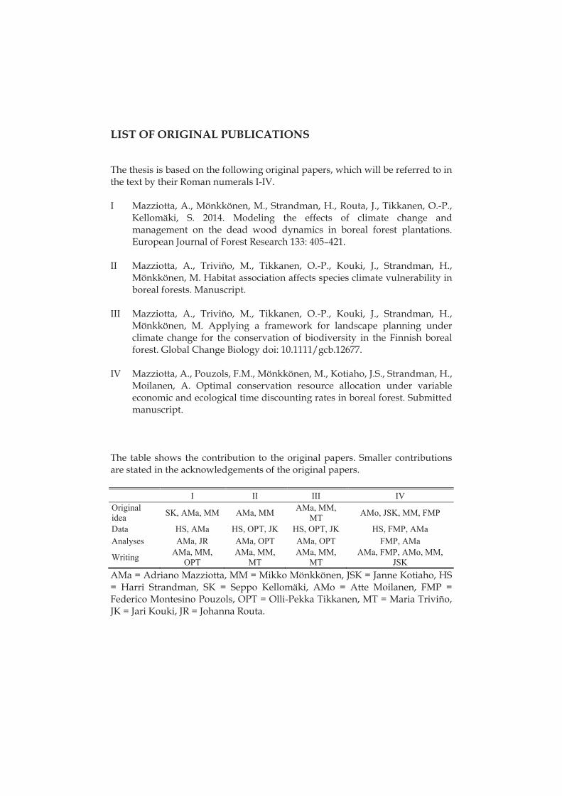
The thesis is based on the following original papers, which will be referred to in the text by their Roman numerals I-IV.

I Mazziotta, A., Mönkkönen, M., Strandman, H., Routa, J., Tikkanen, O.-P.,

Kellomäki, S. 2014. Modeling the effects of climate change and management on the dead wood dynamics in boreal forest plantations. European Journal of Forest Research 133: 405–421.

II Mazziotta, A., Triviño, M., Tikkanen, O.-P., Kouki, J., Strandman, H.,

Mönkkönen, M. Habitat association affects species climate vulnerability in boreal forests. Manuscript.

III Mazziotta, A., Triviño, M., Tikkanen, O.-P., Kouki, J., Strandman, H.,

Mönkkönen, M. Applying a framework for landscape planning under climate change for the conservation of biodiversity in the Finnish boreal forest. Global Change Biology doi: 10.1111/gcb.12677.

IV Mazziotta, A., Pouzols, F.M., Mönkkönen, M., Kotiaho, J.S., Strandman, H.,

Moilanen, A. Optimal conservation resource allocation under variable economic and ecological time discounting rates in boreal forest. Submitted manuscript.

The table shows the contribution to the original papers. Smaller contributions are stated in the acknowledgements of the original papers. I II III IV Original idea SK, AMa, MM AMa, MM AMa, MM,

MT AMo, JSK, MM, FMP

Data HS, AMa HS, OPT, JK HS, OPT, JK HS, FMP, AMa Analyses AMa, JR AMa, OPT AMa, OPT FMP, AMa

Writing AMa, MM, OPT

AMa, MM, MT

AMa, MM, MT

AMa, FMP, AMo, MM, JSK

AMa = Adriano Mazziotta, MM = Mikko Mönkkönen, JSK = Janne Kotiaho, HS = Harri Strandman, SK = Seppo Kellomäki, AMo = Atte Moilanen, FMP = Federico Montesino Pouzols, OPT = Olli-Pekka Tikkanen, MT = Maria Triviño, JK = Jari Kouki, JR = Johanna Routa.

1 INTRODUCTION

1.1 Prelude – The effects of climate change on the biological systems

Climate change alters the spatial, temporal and physiological dimensions of the niche of the species (Bellard et al. 2012). Species respond to climate change by alternatively modifying their distribution range, adapting to the new conditions or going extinct locally or globally (Bellard et al. 2012). Acting in synergy with other anthropogenic threats like habitat destruction and fragmentation climate change represents today an important driver of species extinction, along with environmental variability and invasive species, whose importance is increasing (Brook et al. 2008). These negative effects on species are reflected at community and ecosystem level (Walther 2010) and may alter key processes important to the productivity and sustainability of Earth´s ecosystems (Hooper et al. 2012) and the future delivery of ecosystem services (Montoya and Raffaelli 2010). The rules for conducting a climate-change biodiversity assessment have been already defined (Dawson et al. 2011), and minimizing the loss of biological diversity is still possible following a wide set of recommendations (Heller and Zavaleta 2009). However, considerable uncertainty remains concerning the management actions which should follow these recommendations, and be applicable in a systematic cost-effective way at landscape level, in accordance with the principles of the Convention on Biological Diversity (2010).

1.2 Climate change effects on the boreal forest

Boreal forests are expected to be severely altered by climate change as changes are likely to be faster and of larger magnitude at higher latitudes (Eggers et al. 2008, Ruckstuhl et al. 2008, Lindner et al. 2010, Hickler et al. 2012). According to Solomon (2007) in northern Europe by 2100 an increase up to 6 °C in the annual

10

mean temperature may occur due to the doubling of atmospheric CO2, with an increase in precipitation and changes in seasonal precipitation patterns. The increasing atmospheric CO2 concentration and warmer temperatures are enhancing forest regeneration, growth and mortality (Eggers et al. 2008, Lindner et al. 2010, Hickler et al. 2012), as well as increasing timber harvesting potential (Nabuurs et al. 2007). Growth is further increased by the increase of growing season and the enhanced mineralization of nitrogen bound in dead wood and litter due to warming climate (Bergh et al. 2003, Lindner et al. 2010). However limiting factors may locally reduce growth if there is: (i) low water availability, due to the enhanced evaporation and the reduced accumulation of snow replenishing soil water (Hartmann 2011); (ii) a consistent increase in cloudiness as a feedback from vegetation growth, reducing incoming solar radiation; (iii) heat stress caused by wildfire; (iv) increased probability and severity of pest attack (Dudley 1998, Johnston et al. 2009). Furthermore, the climatic warming is likely to increase the share of deciduous trees in the tree species composition, which will increase the leaf litter with faster decay and mineralization of nitrogen (Bergh et al. 2003). In Finland, tree species distributions are also changing and broadleaved deciduous trees (mainly birch) are expanding northwards while Scots pine (Pinus sylvestris) is increasing its dominance in the less fertile forest types in the south at the expense of Norway spruce (Picea abies) (Kellomäki et al. 2008, Hanewinkel et al. 2013). This is likely due to an expected increase in the frequency of drought episodes in southern Finland, whereas in northern Finland short supply of water is not likely (Kellomäki et al. 2008, Ge et al. 2013).

1.3 Climate change effects on boreal forest species: winners and losers

The following definitions of species vulnerability to climate change and its components (exposure, sensitivity and adaptive capacity), a well-established framework in climate change biology, are quoted from the review paper of Dawson et al. (2011):

“Vulnerability is the extent to which the species is threatened with population decline, reduced individual fitness, genetic loss or extinction owing to climate change”. “Vulnerability has three components: exposure (which is positively related to vulnerability), sensitivity (positively related), and adaptive capacity (negatively related)” (Dawson et al. 2011).

“Exposure is the extent of climate change likely to be experienced by a species. Exposure depends on the rate and magnitude of climate change (changes in the abiotic factors such as temperature, precipitation etc.) in habitats and regions occupied by the species”. “Most assessments of future exposure to climate change are based on scenario projections from General Circulation

11

Models often downscaled with regional models and applied in niche models” (Dawson et al. 2011).

“Sensitivity is the degree to which the survival, persistence, fitness, performance, or regeneration of a species or a population is dependent on the prevailing climate. Sensitive species are likely to show great reductions in survival or fecundity with relatively small changes in climate variables. Sensitivity depends on a variety of factors, including ecophysiology, life history, and microhabitat associations” (Dawson et al. 2011).

“Adaptive capacity refers to the capacity of a species or constituent populations to cope with climate change by persisting in situ, by shifting to more suitable local microhabitats, or by migrating to more suitable regions. Adaptive capacity depends on a variety of intrinsic factors, including phenotypic plasticity, genetic diversity, evolutionary rates, life history traits, and dispersal and colonization ability. Sensitivity and adaptive capacity can be assessed by empirical, observational, and modeling studies” (Dawson et al. 2011).

The degree of climate vulnerability determines whether the species is a winner, i.e. it will gain more habitat/climatic space/resources, or a loser, i.e. it will lose habitats or resources, and face reduced climatic envelope under altered climate conditions.

In the Finnish forests, Tikkanen et al. (2006) estimated that out of the total of 457 red-listed boreal species, about 60% (276 species) are dependent on dead wood for the completion of their life cycle. In order to estimate the climate vulnerability of this complex ecological guild it is important to understand how these species are related to their primary resource, as its alteration determines their sensitivity to climate change. Climate change may result in an increase in the availability of cumulated ‘‘productive’’ energy, i.e., of the energy stored in the tree wood volume, as an effect of the faster forest succession, causing a general increase in species richness (Evans et al. 2005; Honkanen et al. 2010; Reich et al. 2012). This, however, depends on what happens to critical fractions of the resources the species require, as certain decay or diameter classes, and may thus vary among taxa. Out of the red-listed species dependent on dead wood whose association with tree species is known (265 species), in Finland 20 species occur on birch (Betula spp.), 40 species on aspen (Populus tremula), 48 species on Scots pine (Pinus sylvestris), 65 species on Norway spruce (Picea abies), while the rest of the species occur on deciduous trees (42 species are deciduous generalists or associated with Alnus and Salix) or on coniferous trees (50 species).

The abovementioned expected change in tree species composition with global warming (Kellomäki et al. 2008, Ge et al. 2013) will correspondingly modify the survival of red-listed species dependent on them. For example, the reduced success of Norway spruce in southern Finland will likely imply a further endangerment of its associated specialized taiga species and an increase of the more southern species dependent on birch. In general, species persistence will be critically dependent on their ability to disperse and colonize new sites with advancing climate change. The acceleration of growth rate induced by

12

climate change may reduce habitat availability for many specialist saprotrophic wood-fungi (Edman et al. 2006), cambium-living beetles, certain noctuid moths and spiders preferring slow-growing forests (Ehnström 2001).

1.4 Management effects on the boreal forest and its biodiversity

The dynamics and composition of boreal forests have been deeply modified for decades by human activity, i.e. by forestry, especially in Fennoscandia, and this is expected to continue in the future (Nabuurs et al. 2007). Strategies to adapt the current forest management practices to climate change, in order to maximize the profit from forests with altered environmental conditions, include more frequent thinning and reducing forest rotation lengths to utilize the increased productivity (Kellomäki et al. 2008). On the other hand, to maintain biodiversity, future forestry should also ensure availability of coarse woody debris (CWD) at different stage of decay from different forest species (Tikkanen et al. 2006). Even if under climate change the overall habitat availability (amount of dead wood) in boreal forest is expected to increase, dead wood availability will also depend on the management regime applied (Briceño-Elizondo et al. 2006; Garcia-Gonzalo et al. 2007). Intensive timber extraction, which is typical for Fennoscandian production forests, reduces dead wood availability for saproxylic species through thinning, limiting tree mortality preventing dead wood accumulation, and clear-felling (Hynynen et al. 2005; Hjältén et al. 2012; Tikkanen et al. 2012; Gossner et al. 2013). Moreover, a more frequent site preparation (harrowing) may contribute to more rapid dead wood removal, limiting in this way suitable dead wood resources (Ehnström 2001;Schroeder et al. 2007; Rabinowitsch-Jokinen and Vanha-Majamaa 2010). These negative management effects can be remedied by forest protection, which increases habitat availability and releases high dead wood volumes in the landscape by promoting a higher diversity of dead wood stages (Hjältén et al. 2012, Gossner et al. 2013).

1.5 Systematic conservation planning to face climate change

1.5.1 Landscape-level assessment for conservation under climate change

Gilsson et al. (2013) suggest that an assessment of the landscape for conservation under climate change should rely on an estimate of two indicators: conservation capacity (i.e., resilience to change) of landscape patches and their vulnerability to climate change (i.e., sensitivity and exposure sensu Dawson et al. 2011). Landscape conservation capacity can be defined as the ability of the landscape to maintain habitats for species populations and their spatial configuration (connectivity), which both are essential for species persistence

13

(metapopulation viability, Hanski and Ovaskainen 2000). In a landscape context, climate vulnerability depends on the modifications of the landscape induced by climate change (exposure) and how the species will respond to these changes (sensitivity, dependent on the geographic variability of the suitable characteristics of the landscape).

Using this framework we can assess whether or not landscapes provide suitable habitats for species under new climatic conditions. Categorizing landscapes in this two-dimensional space of conservation capacity and climatic vulnerability is helpful in assigning them to relevant conservation actions (Heller and Zavaleta 2009). Four categories of landscape responses to climate change can be identified in the landscape (Heller and Zavaleta 2009; Gillson et al. 2013): a) susceptible, i.e. intact regions highly vulnerable to climate change; b) resilient, i.e. relatively intact areas with low climatic vulnerability that could represent important climate refugia; c) resistant, i.e. regions with low current conservation capacity and with low vulnerability to climate change; d) sensitive, i.e. low current conservation capacity regions but vulnerable to climate change.

1.5.2 Allocation of conservation strategies for biodiversity conservation

The abovementioned systematic planning of the landscape to accommodate adaptation strategies for climate change is an essential tool to efficiently allocate the usually limited budget available for conservation-oriented measures (cf. Lindenmayer et al. 2007, Watson et al. 2013, Alagador et al. 2014). For each element of the landscape for which a certain climate change response category has been identified, it is possible to attribute the correspondent action, as follows: susceptible = management for heterogeneity through conservation; resilient = monitoring and maintenance of conservation capacity; resistant = areas suitable for restoration projects; sensitive = areas where, depending on the intensity of climate change, alternative actions are required: restoration, conservation, or neglect.

Resource allocation to multiple alternative conservation actions is a complex task. A common trade-off occurs between protection of smaller, expensive, high-quality areas versus larger, cheaper, partially degraded areas. In boreal forest, this trade-off realizes between two options: setting aside of mature stands for conservation vs. setting aside of clear-cuts for passive restoration. The allocation of resources into alternative actions to be cost-effective should be optimized in a way that conservation value is maximized in a robust manner in the long run. To achieve this goal an optimization framework (RobOff, Pouzols et al. 2012, Pouzols and Moilanen 2013) can quantitatively identify sets of actions that produce high conservation value that is balanced across features, forest environments and time, guided by costs and budget availability.

14

1.6 Aims of the study

The studies focusing on the effects of anthropogenic climate change on species and ecosystems are increasing at dramatic rate, as these effects become more evident, causing an increasing concern of the society. Despite these efforts many key scientific questions in climate change biology should still be addressed: basic questions examining the alteration of biodiversity patterns and ecological processes induced by the joint anthropogenic changes in climate and environment; applied questions related with the strategies for adaptive management under climate change guaranteeing the future provision of ecosystem services. In this intricate set of challenges, my thesis analyses: (1) the causal relationships between climate change and a specific biome, the boreal forest, also in response to the disturbance provoked by forestry at local level, in southern and northern Finland, through a single forest rotation (I); (2) the effects that an altered forest dynamics will have on the provision of habitat for its biodiversity at country level, in Finland, by the end of the 21st century (II); (3) the level of resilience of the forest landscape to climate change and the consequent suite of conservation actions to apply to increase resilience at country level, in Finland, by the end of the 21st century (III); (4) the optimal allocation of conservation actions in forest landscapes for long-term ecological and economical sustainability when limited economic resources are available at regional level, in southern Finland through a long-planning horizon (300 years) (IV).

2 MATERIALS AND METHODS

2.1 Forest ecosystem simulator

2.1.1 The SIMA model (I, II, III, IV)

I simulated the dynamics of forest stands by employing the ecosystem model SIMA which has been successful in previous studies in predicting the effects of the changing climate on the forest succession (Kellomäki et al. 1992a,b, Kölstrom 1998, Kellomäki et a. 2008). SIMA is a non-spatial gap type model, in between a pure physiological model and a statistical one, based on the properties of individual trees and utilizing a time step of one year. In the model, regeneration is partly stochastic and partly controlled by the availability of light, soil moisture and temperature. The growth of trees is based on the diameter growth, which is the product of the potential diameter growth and environmental factors as regards temperature sum, within-stand light conditions, soil moisture, and the availability of soil nitrogen. These factors control the demographic processes (recruitment, growth, death) of tree populations.

Litter and dead trees are decomposed into soil with subsequent release of nitrogen bound in soil organic matter. The litter cohort indicates the amount of dead material originating from trees and ground vegetation annually. The weight loss of a litter cohort is a function of the current ratio between lignin and nitrogen and it depends on the available soil moisture and the level of canopy closure. The mineralization process of nitrogen depends on the nitrogen-carbon ratio of the humus and on the local climatic conditions (Pastor and Post 1986). Simulations are based on the Monte Carlo simulation technique, i.e. certain events, such as tree recruitment and death, are partly stochastic. Each time such an event (e.g., death of an individual tree) is possible, the algorithm selects whether or not the event will take place by comparing a random number with the probability of occurrence of the event. The model has been previously validated with forest inventory data in Kolström (1998), Kellomäki et al. (2008) and Routa et al. (2011).

16

2.1.2 Climatic scenarios (I, II, III, IV)

I performed the simulations of forest succession with SIMA by applying the baseline climate (for all the papers) and (for the papers I, II and IIII) three scenarios of increasing emissions of the Intergovernmental Panel on Climate Change (IPCC) for changing climate (low emissions, B1; intermediate, A1B; high, A2) (Nakicenovic et al. 2000). In paper IV I applied only the baseline scenario for the whole time horizon of 300 years, in order to avoid the confounding effect of alternative climate change scenarios on the main problem of resource allocation to alternative conservation actions. I used six climatic variables (temperature sum, number of dry days, evaporation, evapotranspiration, mean monthly temperature and precipitation) covering the entire Finland area from the Finnish Meteorological Institute (Kellomäki et al. 2008). The baseline climate was calculated at a resolution of 10 km for the period 1971–2000, whereas future climatic projections were calculated at a resolution of 49 km for the period 2010-2099. Then, all variables were spatially joined to the grid of the National Forest Inventory (grid size of 16 km in southern Finland and 32 km in northern Finland, see below) (Venäläinen et al. 2005, Jylhä 2009). In both cases, the climatic data represented the daily values over the seasons introducing the inter-annual variability around the trends in the climatic variables. The interannual variability was obtained using the monthly mean temperature and precipitation with the standard deviations for the rotation time (tri-decadal averages and standard deviations).

Regarding the atmospheric CO2, the annual mean values were used in the simulations. Under the baseline climate, the atmospheric CO2 was a constant of 352 ppm, whereas under the changing climate the CO2 increased from the baseline one, with concurrent changes in temperature and precipitation, based on the IPCC scenarios. Low emission scenario (B1), assumes a global environmentally sustainable development, and can therefore be considered the least plausible scenario. In B1 scenario emissions increase until 2020 at a much lower level than in the other scenarios followed by a stable emission period up to 2040, and a decrease close to zero emission levels by the end of the century. B1 is predicted to be associated with + 1.1 - +2.9 °C global increase in temperature. Intermediate emission scenario (A1B) assumes rapid economic growth but in a more globalized world balancing the use of all energy sources (included renewables). A1B assumes an increase in the emissions up to 2050 approximately at the same pace as A2 scenario, followed by a decrease in emissions to the 2020 levels by the end of the century. A1B predicts +1.7 - +4.4 °C increase in global temperature. High emission scenario (A2) assumes a more divided world with regionally oriented economic development with a delayed use of renewable energy, and a continuous increase in the emissions up to the end of the century. It will be associated with a global average surface warming until 2100 between +2.0 and +5.4 °C).

Ecosystem models have widely been used in determining how environmental factors (like temperature, light, soil nitrogen and moisture) influence the demographic processes (birth, growth and death) in tree

17

populations. Furthermore, ecosystem models provide tools to analyse how management and climate change may effect on the dynamics of tree populations and dead wood in the succession of forest ecosystems (LeMay and Marshall 2001, Landsberg 2003).

At different spatial scales, the model approaches vary substantially from each other depending on applications. At global scale, Dynamic Global Vegetation Models (Cramer et al. 2001 for an overview of DGVMs) are useful if a rather coarse spatial resolution is used in identifying the climate change effects on the boreal forests as a whole and the processes involved in the decay of dead wood (McDowell et al. 2011). However, the spatial extend in my thesis varies from stand to regional level at which DGVMs are not appropriate. At more local scale, gap-type models, like the SIMA model applied in this thesis, allow conducting detailed population-level analysis about: (i) the interaction between growth and mortality, (ii) the consequent dynamics of dead wood and its decomposition, (iii) the consequent availability of resources for different forest species.

2.1.3 Individual level simulations (I)

I ran these simulations in two locations, one in southern and one in northern Finland. In both cases, I did the simulations across a fertility gradient corresponding to the presence of certain ground vegetation in the sites, in accordance with the Cajander (1949) classification of the following forest types: a) herb rich type (Oxalis-Myrtillus, OMT), heath forests, with Norway spruce as dominant species with admixtures of birch, b) bilberry type (Myrtillus, MT), mesic heath forests with a mixture of Norway spruce, birch and Scots pine; c) cowberry type (Vaccinium, VT), sub-xeric heath forests and d) lichen type (Calluna, CT), xeric heath forests where the main tree species is Scots pine (Cajander 1949). Details about the relationships among site types and soil characteristics (classification, water holding capacity, fertility) and on the initialization of the simulations are described in Kellomäki et al. (2008). The stands were of single species with the initial mean diameter of 2 cm at the height of 1.3 m above the ground level. Totally, 48 initial stands were used in the simulations, which included two management regimes.

In the first management regime, no thinning or clear cutting was done excluding any timber/biomass harvest (set-aside regime (SA)). In the second management regime, the current recommendations (Yrjölä 2002) were applied (business-as-usual (BAU). This involved thinnings one to two times per rotation. After thinnings, noncommercial residual biomass was left above ground. When BAU was used, a clear cut harvesting leaving 5 retention trees per hectare was done at the end rotation. In applying SA and BAU regimes, any abiotic and biotic disturbances were excluded. In both cases, the rotation/monitoring period was 80 years. The simulations were repeated 20 times for each of the 192 combinations of tree species, climate, management regime, forest type, density and region in order to determine the central

18

tendency of variations (average values) in the time behavior of the forest ecosystem.

2.1.4 Stand level simulations (II, III, IV)

I performed stand level simulations of forest dynamics by employing data from the Finnish National Forest Inventory (NFI). The NFI is provided by the Finnish Forest Research Institute (METLA) and contains information about the composition (tree species, site type) and structure (age class, diameter) of forest stands as well as key statistics on Finland´s forests, forestry and forest industries. Sample forest plots of 100 m2 are systematically distributed in a permanent grid all over Finland. The grid size of the plots is 16x16 km2 in southern Finland and 32x32 km2 in northern Finland. In my study I simulated data from the 9th NFI originating from 1996-2003 data (Finnish Forest Research Institute 2010). All study plots are located on upland mineral soils. In the 9th NFI, 65% of the NFI sites were on mineral soil and 35% on mires. Most of them belong to site types of high, medium or low fertility. In every case the simulations were repeated 10 times in order to determine the central tendency of variations in the time behaviour of the forest ecosystem. The model was run on an annual basis.

Forest dynamics was simulated by applying different management practices, depending on the aim of the paper:

Papers II and III: I applied in these studies the current Finnish management policy consisting of two different practices: (i) set-aside (SA), no management on the stands located within current public and private protected areas, to guarantee natural forest succession (applied in 3% of the total NFI plots); (ii) Business-As-Usual (BAU), recommended management for maximizing timber volume extraction (Yrjölä 2002) applied outside the protected areas (97% of the NFI plots). Details for the application of rules for thinning and clear-cut are given in Kellomäki et al. (2008). The initial planting density was 2000 saplings / ha throughout the country, regardless of the tree species and site type. In order to homogenize the treatment, the deterministic application of management rules was replaced by a random procedure, with no major change in stocking at the beginning of the simulation (Kellomäki et al. 2008). Here a typical rotation period of 90 years for each stand was applied.

Paper IV: I examined cost-effective allocation of resources into three alternative actions applied to mature forest stands in southern Finland: current standard forest management rules (business-as-usual), set-aside and protect as mature stand (SA), clear-cut followed by set-aside and protection (CC+SA). In both set-aside scenarios (SA and CC+SA), natural succession was assumed to follow; in CC+SA after the forest first has been cleared during the first 30 years. Here I chose a time frame of 300 years, corresponding to about 4 rotations, to guarantee the stands subject to CC+SA to reach a maturity status through succession comparable to the one reached in old-growth forests in SA.

19

2.2 Measuring habitat availability (II, III, IV)

I extracted habitat suitability responses for ecological guilds and threatened species from SIMA simulations. This was done by translating structural characteristics of stands into potential stand suitability for species sharing certain ecological preferences, via sub-utility functions. I calculated the Habitat Suitability Index (HSI) as the product of different sub-utility functions. HSI changes through time as a function of the management scenario applied in the forest stand. The HSI indexes vary between 0 (unsuitable) and 1 (optimal habitat) and can be alternatively considered either as a proxy for habitat suitability for ecological groups or as proxy for probability of occurrence of the focal species (Mönkkönen et al. 2014).

I calculated HSI as the product of the following sub-utility functions: - Paper II and III: here the HSIs for habitat associations of threatened

species (beetles and fungi) associated with dead wood (see paragraph 2.4) are derived by two sub-utility functions for microclimate and resource quality. Microclimate is a function of the basal area of the living stock of stand. The resource quality is a function of three components of dead wood: tree species, decay stage, diameter preference (Tikkanen et al. 2006, 2007).

- Paper IV: here HSIs are calculated for six focal species (birds and mammals, see section 2.4) with species-specific sub-utility functions related with different stand characteristics: tree volume, dead wood volume in different decay stages, tree density, tree basal area, stand age, proportions of volumes for certain tree species in the stand.

2.3 Measuring conservation capacity and climate vulnerability (II, III)

I calculated an estimate of the potential stand (the landscape unit) conservation capacity (SCC) for each NFI sample plot by weighting the habitat suitability across the k ecological groups, as follows (cf. Pakkala et al., 2002):

HSIs is the habitat suitability index (HSI) calculated under a certain s climatic scenario. The current was calculated under baseline climate conditions projected and averaged across the first 3 simulated decades of the 21st century (t = 2010-2039) for each species group k. SCCs is thus the weighted average of group specific HSI, the weights being the HSIs themselves. This puts more emphasis on large HSI-values than mere average. SCCs scales between 0 and 1, where 0 denotes low and 1 high conservation capacity for all species groups.

20

I calculated Climate vulnerability (CV) as a measure of the variation in SCC induced by climate change. CV was calculated for each NFI sample plot by subtracting to the SCCs calculated under stationary climate (s = SC) conditions the SCC alternatively calculated under the three climate change scenarios (s = B1, A1B, A2), as follows:

Habitat suitability indices (used in the calculation of SCC) under stationary and altered climate were averaged across the last three simulated decades of the 21st century (t = 2070-2099), when the effects of climate change on forest dynamics are predicted to be the highest (Kellomäki et al. 2008). A negative CV value corresponds to an increase in SCC induced by climate change (improved landscape quality), a positive CV value to a decrease in SCC under climate change (landscape degradation). Original CV values vary between 0 and 1. Original values were further slightly modified to put more emphasis on changes in values in the middle of the gradient (values around 0.5; see II and III for motivation), and finally, re-scaled between 0 and 1.

2.4 Defining winners and losers under climate change (II)

In the species assessment, we categorized species into winners if their average CV across all NFI stands belonged to the lowest quartile of the values and losers when CV was in the highest quartile; all other species were considered stable typically having both negative and positive CV values. We scrutinized the resources and micro-climatic preferences making species particularly susceptible to climate change. Further, spatial turnover in species habitat was calculated as the absolute sum of the positive and negative variations in the CV values. We categorized species as having low spatial turnover if their absolute CV sum across all stands belonged to the lowest quartile of the values and having high spatial turnover when CV was in the highest quartile; all other species had intermediate turnover. A low level of turnover was considered desirable as it means a low level of spatial rearrangement of habitat across the landscape. Finally the separate effects of sensitivity (species habitat association) and exposure (projected rate of climate change) on climate vulnerability were evaluated using Generalized Linear Models (GLMs) for each emission scenario.

2.5 Defining response categories under climate change (III)

I categorized the Finnish NFI sample plots based on their response to climate change. This was conducted by allocating them in a bi-plot, on the basis of their values for the SCC and the CV, in accordance with the classification proposed

21

by Gillson et al. (2013, as follows: a) susceptible plots (with SCC > 0.5 and CV > 0): the most intact forest landscapes vulnerable to climate change, requiring management for heterogeneity and resilience; b) resilient plots (with SCC > 0.5 and CV < 0): intact areas with low climatic vulnerability potential climate refugia requiring conservation capacity maintenance; c) resistant plots (with SCC < 0.5 and CV < 0): low current conservation capacity landscapes with low climatic vulnerability suitable for restoration projects; d) sensitive plots (with SCC < 0.5 and CV > 0): low conservation capacity landscapes and vulnerable to climate change where alternative conservation measures are required depending on the intensity of climate change. I obtained the magnitude of each response category for each plot by calculating the absolute value of the product between SCC under stationary climate and CV of each climate change emission scenario. I described the main patterns in the occurrence and magnitude of climate change response categories with alternative emission scenarios and across the boreal vegetation zones.

2.6 RobOff, decision support framework in conservation planning (IV)

I applied the RobOff framework and software (Pouzols et al. 2012, Pouzols and Moilanen 2013), which derives its name from robust offsetting, to optimally allocate conservation resources into multiple alternative management actions. The core of this framework emphasizes the uncertain responses of different biodiversity features to alternative management scenarios in different habitat types or environments. Responses over time of biodiversity features to different management actions are the main input of RobOff. In this application, biodiversity responses were the trends of the HSI values for six focal species. The responses were specified in a RobOff framework setup as estimated values and upper and lower uncertainty envelopes (calculated as 95% confidence intervals, accounting for inter-stand variability) for each decade across 300 years. The three alternative management options applied in three different forest types were modeled as nine different actions, each having different costs and producing different responses of biodiversity features. Thus, a total of 54 different responses were defined (six focal species × three forest types × three management scenarios). Additional data objects considered in RobOff are the costs of conservation actions (or Net Present Values of alternative management options), and the budget available. The budget used corresponds to the amount of funding for additional forest conservation in southern Finland through the METSO II program over a period of five years (Ministry of the Environment 2008) and its multiplications.

In the framework, different discount rates were applied both to the HSIs and to the economic value to deal with differential time preferences for economic and ecological values. Present time economic returns from timber

22

harvesting are generally valued higher than returns that can be harvested sometime in the future. Accordingly, we only allowed positive discount rates for economic value, +1%, +3%, and +5%. In contrast, opinions about ecological discounting vary, and it has been proposed that the future could be valued equally or even higher than present (Gollier 2010, Kula and Evans 2011). Thus, a wider range of discount rates was allowed for ecological value (-5%, -3%, -1%, -0.5%, 0%, +0.5%, 1%, 3%, 5%). If the discount rate is negative, the future is valued more than the present. We used the exponential model for discounting NPV and a quasi-hyperbolic model with a constant rate for discounting ecological values (Green and Myerson 2004).

2.7 Threatened and focal species

2.7.1 The HERTTA database (II, III)

I calculated HSIs for analysing the effects of climate change and/or management at different scale: at stand level I employed data of threatened saproxylic species from the Environmental Information System of the Finnish environmental administration (Hertta), at landscape level, in order to evaluate the effects of forest management, I used information about the potential suitability of certain stand characteristics for six vertebrate focal species.

Hertta is based on the data updated to 2013 including 25,515 records for 129 species: 64 Coleoptera and 65 Fungi (Rassi et al. 2000). Threatened saproxylic species are considered as sensitive indicators of the good quality of the forest, being able to survive only with reasonably high amounts of dead wood in the stand ( 20m3/ha), therefore favourable conditions for species survival in the stands can guarantee the persistence for many other saproxylic species inhabiting the boreal forest. I attributed ecological characteristics to the threatened species on the basis of the habitat associations reported in the Hertta database.

2.7.2 Focal species (IV)

Here I chose six focal species (birds and mammals) representing the most important dimensions of variation in boreal forest diversity and a wide spectrum of habitat associations, responses to management, and conservation and social values (Mönkkönen et al. 2014):

Capercaillie (Tetrao uralensis) is a game bird with a high social and economic value. It has also conservation value being listed as near threatened in the latest National red-list of Finland (Rassi 2010) and it is considered umbrella species for overall species richness of breeding forest birds and game animal richness (Pakkala et al. 2003). Capercaillie leks are typically situated in pine-dominated semi-open mature forests with spruce understorey (Miettinen et al. 2010).

23

Hazel grouse (Bonasia bonasa) is also a game bird, and suggested to be an indicator of adequate level of deciduous tree mixture in conifer dominated boreal forest landscapes (Angelstam 1992) favouring dense cover below the canopy (Angelstam et al. 2004).

The three-toed woodpecker (Picoides tridactylus) is a conifer forest species dependent of recently dead or dying wood and also suggested as an indicator species for overall species richness of forest birds (Pakkala 2012).

The lesser-spotted woodpecker (Dendrocopos minor) is a red-listed bird species associated with deciduous, often mid-successional forests and dependent on recently dead or dying wood (Wiktander et al. 1992).

The long-tailed tit (Aegithalos caudatus) prefers middle-aged to old forests dominated by deciduous trees, where they feed on insects in the canopy (Jansson and Angelstam 1999).

The flying squirrel (Pteromys volans) is a threatened (vulnerable, Rassi et al. 2010) species associated with mature spruce dominated mixed forests (Mönkkönen et al. 1997) and an umbrella of overall species diversity in spruce forest stands (Hurme et al. 2007).

3 RESULTS AND DISCUSSION

3.1 Effects of climate change and management on dead wood dynamics (I)

3.1.1 The effects of region, forest type, density and climate change

I confirmed the positive effect of lower latitude, forest types of increasing fertility and higher initial tree density in accelerating tree growth and dead wood dynamics (Pretzsch 2010, Pretzsch et al. 2013, Pretzsch et al. 2014). As expected from previous research, climate change enhanced the growth, increased the annual input and volume of dead wood, finally accelerating the decomposition (Kellomäki et al. 2008, Shorohova et al. 2008, Woodall and Liknes 2008, Zell et al. 2009, Tuomi et al. 2011). On the other hand in my study climate change had direct effect on increasing the mortality rate as such for Scots pine and Norway spruce, as observed by Harmon (2009) and McDowell et al (2011), while reducing mortality in silver birch. The simulated increase in tree growth is explained by the contribution of climate change in enhancing the mineralization of nitrogen, via an increased evapotranspiration, given the high soil water content. However this general trend was not confirmed for Norway spruce, for which growth in southern localities decreased under climate change, probably as a response to drought, whereas in the north growing conditions will likely improve, confirming the results of Kellomäki et al. (2008) and Ge et al. (2013). In general climate change provokes an earlier culmination of diameter growth and enhanced maturation and the reduction of growth in older and larger trees (Harmon 2009). This explains why the enhanced growth indirectly increased the annual input of dead wood. At the same time, the decomposition of dead wood was enhanced, but the increase was smaller than that of the dead wood input. Consequently, in my simulations climate change increased the accumulation of dead wood.

25

3.1.2 The effect of management

I found that the management regime (no thinning/thinning) was a more important driver than climate in altering the growth and mortality and the consequent amount of dead wood in the site regardless of location and tree species, confirming the results of Shanin et al. (2010), Hjalten (2012) and Gossner et al. (2013). This was expected because more space is created in thinning for remaining trees thus avoiding too early reduction of growth and the consequent death. On the other hand, thinning was done from below, thus removing the suppressed trees, which are most susceptible for death due to reducing growth. Thinning reduced substantially the dead wood input and increased the decomposition rate of coniferous dead wood while increasing the decomposition rate of silver birch. In these respects the exclusion of thinning increased dead wood input substantially boosting the accumulation of dead wood for all the tree species, but while for coniferous trees the retention time of dead wood was increased by a slower decomposition rate, for silver birch accumulated dead wood had a faster turnover (cf. Briceño-Elizondo et al. 2006; Garcia-Gonzalo et al. 2007). For all the tree species under climate change the BAU regime will provide lower increase in annual input of dead wood respect to the SA regime. This input of dead wood will be decomposed faster under SA regime for silver birch, while for Norway spruce set aside will reduce the increase in decomposition, guaranteeing the persistence of the vanishing Norway spruce dead wood, especially in the south.

3.1.3 Consequences for forest biodiversity

I confirmed that in the boreal forest, climate change is likely to increase the tree wood volume, likely causing a general increase in species richness (Evans et al. 2005, Honkanen et al. 2010; Reich et al. 2012). My simulations showed that climate change is likely to increase the total volume of dead wood available for forest dwelling species, despite an increased decomposition rate. The increase in dead wood will likely provide more resources and improve habitat availability, especially for the red-listed species dependent on dead birch and Scots pine trees. According to my study under climate change in average dead wood volumes will meet the thresholds of 20-40 m3 recommended to sustain populations of the majority of the threatened species in boreal forest (Müller and Bütler 2010, Junninen and Komonen 2011). On the other hand my results show that forest management can reduce the amount of dead wood, as already observed by Shanin et al. (2010), Hjältén et al. (2012) and Gossner et al. (2013). This reduction can be stronger in regions at higher latitudes and on forest types of low fertility. This is relevant when considering that, in general, poorly productive areas that are marginally good habitats for species have been often chosen in boreal forest for settlement of protected areas (Nilsson and Götmark 1992, Virkkala and Raijasärkkä 2007). For the highest contingent of red-listed species associated with Norway spruce my simulations predicted a slight increase (+26%) in the availability of dead wood with climate change. The

26

adaptation strategies for Norway spruce under climate change consider planting cultivars of more southern provenance for regeneration (Kellomäki et al. 2008, Weslien et al. 2009) and planting Norway spruce on sites that are edaphically most favorable for it (Ge et al. 2013). However my results show that the persistence of Norway spruce dead wood in the landscape can be guaranteed by setting aside stands, counterbalancing the strong increase in decomposition rate induced by climate change.

My study shows that climate change influences the processes regulating dead wood dynamics but with different intensity for different tree species. Also the tempo and mode of many of the forest processes is dramatically changing. The retention time of the dead wood stock on the soil will be reduced by an increased decomposition rate for silver birch and Norway spruce. My results confirm an increased growth rate as a consequence of climate change, which is likely to have a negative impact on the habitat availability of species preferring slow-growing wood (Ehnström 2001, Edman et al. 2006).

3.1.4 Adaptation strategies

Even though I showed that the annual input of dead woody material may be higher in future forests, from species perspective this may still mean reductions in habitat availability if economic efficiency and thorough higher thinning rate (Alam et al 2008, Kellomäki et al 2008) is emphasized. My results suggest that the most effective single strategy to provide more dead wood resources for saproxylic species under climate change is to grow stands unmanaged (unthinned). This would ensure larger amounts of dead wood and reduce the decay (turnover) rate of conifer trees, thus providing a more stable resource base for saproxylic organisms. This should be economically sustainable first because Tikkanen et al. (2012) showed relatively low costs (reductions in growth) from growing stands unthinned, and in some cases, refraining from thinnings was also economically a better option. Secondly, the improved growth would make it economically sustainable to leave at least a part of stands without management and still maintain the current timber flow.

3.2 Climate vulnerability (II)

3.2.1 Influence of sensitivity and exposure

Assessing species climate change-vulnerability of species already threatened has been conducted for a very limited portion of biodiversity (Foden et al. 2013). Our knowledge of the impact of climate change on less visible species is often based only on exposure to climate change, even if species sensitivity plays a key role in determining climate change vulnerability (Dawson et al. 2011, Arribas et al. 2012, Summers et al. 2012, Foden et al. 2013, Triviño et al. 2013, Garcia et al. 2014). Here I analyse the role of species sensitivity, represented by habitat

27

associations, in affecting climate change-vulnerability for two less visible species-rich taxonomic groups (coleopteran and fungi) depending on dead wood in the Finnish boreal forest at landscape scale.

3.2.2 Climate vulnerability across species and stands

In accordance with previous studies addressing climate vulnerability for many species (Summers et al. 2012, Foden et al. 2013 Triviño et al. 2013, Garcia et al. 2014), I found an overall reduction in habitat quality induced by climate change for ~30-36% of the threatened dead wood-associated species occurring by the end of the 21st century, while the species improving their habitat quality were only a smaller fraction (~16-22%). However, I found an improvement in habitat quality for >50% forest stands, most likely caused by the higher increase of dead wood caused by an increase in tree growth under higher emission scenarios (Kellomäki et al. 2008). Nevertheless I also found a strong decrease in stand habitat quality for about 40% of stands, which could be explained by an increased decomposition rate (Shorohova et al. 2008; Tuomi et al. 2011) and more frequent harrowing (i.e., site preparation practices) (Rabinowitsch-Jokinen and Vanha-Majamaa 2010; Hautala et al. 2011) likely to contribute to more rapid dead wood removal. The faster dead wood dynamics will likely provide less time for forest species to use the higher volumes of resources produced under climate change (cf. Eggers et al. 2008). Intensive timber extraction, which is typical of Fennoscandian production forests, reduces dead wood availability through thinning and clear-cutting (Hynynen et al. 2005; Tikkanen et al. 2012). In contrast, forest protection increases habitat availability (the amount of dead wood) by favouring a higher diversity of dead wood stages (Hjältén et al. 2012; Gossner et al. 2013).

3.2.3 Habitat associations for winners and losers

I observed a negative trend for threatened species associated with Norway spruce under high (A2) emissions. This is likely a consequence of the predicted reduction of occurrence of this tree species, especially in southern Finland (Kellomäki et al. 2008) and generally in Europe (Hanewinkel et al. 2013), as an effect of the drought-induced enhanced mortality. On the other hand, I observed a positive trend in species associated with Scots pine and deciduous trees, likely a consequence of the predicted enhancement of annual growth for these tree species in Finland (Kellomäki et al. 2008). Losers were more often than winners associated with well-decayed dead wood, as this resource vanished for the reduction of retention time of the dead wood stock on the soil under climate change. The causes for this reduction are an increased decomposition rate and a shorter rotation time to adaptively exploit the increased productivity under climate change (Eggers et al. 2008, Kellomäki et al. 2008). On the other hand, I estimated that species associated with fresh dead wood will be winners under climate change as an effect of predicted higher availability of this resource.

28

3.2.4 Spatial turnover and habitat associations

Little turnover is desirable as it means spatial stability in habitat configuration and thus requires less dispersal for species persistence. I found that spatial turnover in habitats can be a problem for a large proportion of all threatened species likely reducing the possibilities for future adaptation (Arribas et al. 2012), because many forest-dwelling species are considered poor dispersers (Ranius and Roberge 2011). Especially worrisome is the situation for threatened species associated with well-decayed dead wood expected to be menaced both by reduction in habitat quality and high levels of spatial turnover. On the contrary, species associated with Scots pine and deciduous trees even if they were characterized by high levels of spatial turnover were either winners or losers in different stands.

3.2.5 Components of climate vulnerability

The relative importance that climatic exposure and ecological sensitivity have in determining climate vulnerability depends on the scale. In general at landscape/regional scale exposure has a larger importance than sensitivity, while it is the opposite at local scale (Arribas et al. 2012, Summers et al. 2012, Bradshaw et al. 2014, Garcia et al. 2014). By contrast, at the regional scale, I found that sensitivity, i.e. habitat association, accounted for much higher proportion of the variance in climate vulnerability than exposure to local climate conditions. Evidently, whether exposure or sensitivity is driving species climate vulnerability varies not only across scales, but also among taxa and perhaps among ecosystems. In my case, the strong species dependence by habitat associations may be explained by the fact that most of them are strictly dependent on the local microclimatic conditions created in dead wood, which isolate them from the effects of climate change at landscape level (Bradford et al. 2014).

3.3 Climate change assessment of boreal forest (III)

3.3.1 General considerations

My modelling approach provided a climate change assessment of the boreal forests in Finland, overcoming the shortcomings pinpointed by Watson et al. (2013). Indeed I identified categories of response (1) for a forest ecosystem under different scenarios of climate change (2) in a spatially-explicit way (3) taking into account two out of three components of climate vulnerability (exposure and sensitivity). In my assessment these challenges are tackled as follows: (1) accounting for the response at ecosystem level is possible because the simulator provides information about potential suitable habitat for forest species given certain conditions of the forest stands. Stand conditions directly

29

derive from the population parameters during the forest succession, which are influenced by the applied climatic scenario and the forest management; (2) mapping the pattern and magnitude of each response category is conducted at the level of phytogeographic zones; moreover both conservation capacity and vulnerability are based on metrics calculated at the level of the landscape unit, the stand; (3) calculating climate vulnerability accounts at the same time for the exposure of stands, because the effects of climate change on stand conservation capacity varies with geographic location, and their sensitivity, because different ecological groups respond differently to climate change effects.

3.3.2 Conservation capacity and climate vulnerability

I found that the overall conservation capacity of boreal forests in Finland was rather low. This is evidently due to intensive management for timber extraction, which has been shown to have strong negative effects on biodiversity (Mönkkönen 1999), and in particular, on resource availability of species associated with dead wood (cf. Chapin et al. 2007, Ranius and Roberge 2011; Stockland et al. 2012). Conservation capacity will likely remain low if no additional actions, such as restoration measures, are taken to increase it in the future. The low current conservation capacity was particularly prominent for forests in northern boreal zone. Indeed, forests in the southern vegetation zones are currently characterized by a larger proportion of deciduous trees, harbouring higher habitat diversity, and hence larger potential to host species than forests in the north (Tikkanen et al. 2009). Low current conservation capacity and a strong decrease in conservation capacity expected by the end of the 21st century are worrisome, because climate change effects on biodiversity will likely be stronger in landscapes subject to intensive human land-use (Travis 2003; Bomhard et al. 2005; Brook et al. 2008; Barbet-Massin et al. 2012). Management strategies like set-aside are likely to limit the negative climate change effects on biodiversity of production forests (cf. Chapin et al. 2007; Driscoll et al. 2012).

Climate change is expected to have a stronger effect at higher latitudes and to produce more dead wood in the northern boreal zone. However, because of the productivity gradient from higher to lower latitudes, we would expect higher dead wood volumes in central-southern boreal forests than further north and, as a corollary, higher stand conservation capacity for forest dwelling species (Kellomäki et al. 2008). An increased decomposition rate (Shorohova et al. 2008, Tuomi et al. 2011) and more frequent harrowing (i.e. site preparation practices) (Rabinowitsch-Jokinen and Vanha-Majamaa 2010, Hautala et al. 2011) are likely to contribute to a faster dead wood removal. The faster dead wood dynamics will likely provide less time for forest species to use the higher volumes of resources produced under climate change (cf. Eggers et al. 2008).

30

3.3.3 Climate change response categories and adaptation strategies

The application of Gillson´s (Gillson et al. 2013) conservation framework, through the categorization of the landscape, enables suggestions about which areas should be selected for applying different adaptation strategies. In synthesis, my results indicate that irrespectively of the emission scenario the Finnish landscape will likely be dominated by a very high proportion of sensitive and susceptible forest patches whilst resilient and resistant patches maybe relatively rare in the landscape. This means that most forests, irrespectively of their conservation capacity, will be vulnerable to climate change, strongly reducing the prospects for species persistence and for their potential adaptation to new climates. This increased fragility of the landscape translates into a higher uncertainty for landscape managers in the choice of conservation strategies to adopt. However, the magnitude of sensitive and susceptible plots will likely be the lowest under the low emission scenario (B1), intermediate under the high emissions (A2) and the highest under the intermediate emissions (A1B). On the other hand, the magnitude of resilient and susceptible plots is similar under different emission scenarios.

From the point of view of biodiversity conservation, an ideal situation would be to have a high proportion of resilient forests. My results show that their frequency in current landscapes is very low irrespective of the emission scenario, and thus many alternative and drastic conservation actions are needed to improve the situation. In the few resilient patches, which can act as potent important climate refugia, conservation actions, from selective logging to full protection (set-aside) (Chapin et al. 2007), for maintaining the high landscape conservation capacity and monitoring should be delivered (Heller and Zavaleta 2009, Gillson et al. 2013, Watson et al. 2013) across all the vegetation zones under a low (B1) and high (A2) emission scenario, more in the southernmost boreal zones under intermediate (A1B) emissions.

In susceptible patches conservation actions for maintaining high conservation capacity and enhancing heterogeneity, and thereby resilience, through protecting biodiverse forests through permanent or temporary reserves is recommended (Mönkkönen et al. 2011). While under low (B1) emissions protection is needed in all the vegetation zones, under intermediate (A1B) and high (A2) emission scenarios protection would be more required in the northern boreal zone.

The few resistant patches are recommended for restoration projects, which should improve their habitat quality and enhance connectivity in order to turn them into resilient patches (Halme et al. 2013). These measures would increase the reservoir areas for forest species where the velocity of climate change is less critical and adaptation is still possible in all the vegetation zones.

Sensitive stands require alternative measures but achieving resiliency may be difficult as both conservation capacity and climatic vulnerability should be managed. This is easiest for sensitive areas that show relatively low vulnerability and relatively high conservation capacity. Such forests requiring restoration to improve conservation capacity and management for

31

heterogeneity to reduce vulnerability would be more common under a low (B1) emission scenario especially in the northern boreal zone. At the opposite end of the continuum are the highly sensitive patches (very vulnerable and low conservation capacity). These are particularly common under the intermediate (A1B) emission scenario and in the southernmost boreal zones. For such forests, neglect is often suggested to effectively allocate scarce conservation resources elsewhere (Heller and Zavaleta 2009, Gilsson et al. 2013, Watson et al. 2013, Alagador et al. 2014). As an alternative to abandonment in highly sensitive forests especially in the southernmost boreal zones, I recommend setting aside clear-cuts to complement more traditional conservation of old forests: indeed acquiring such stands for conservation purposes is relatively inexpensive and given enough time their conservation capacity will improve.

3.4 Optimal conservation resource allocation in the boreal landscape (IV)

I found that optimal allocation of resources between two management options, i.e. clear-cut followed by set aside (CC+SA) and setting aside of mature forests (SA), strongly depends on discount rates assumed for economic and ecological returns. With the present budget CC+SA becomes relevant already with economic discount rates >2%, a rate lower than generally accepted in economics. Differences in allocation result in varying fractions of the landscape under conservation; this area is large when resources mostly go into CC+SA, which has relatively low opportunity costs per hectare. With the actual budget level, highest investment into CC+SA occurs when we emphasize immediate economic returns (i.e. high economic discount rate) and distant ecological returns (i.e. negative ecological discount rate). Then, a maximum of 4.2% of the focal landscape could be set aside. With increasing emphasis on immediate ecological returns (i.e. increasing ecological discount rate) the relative utility of setting aside mature forests increases, but simultaneously, total area under protection decreases dramatically (maximum 1.4% with the current budget). Decreasing economic discount rates always result in less area set aside due to increased per-area costs of conservation via higher NPV. The relative utility of setting aside clear-cuts and mature forests varies significantly between the species, reflecting species-specific habitat requirements.

My analysis showed that when a longer time perspective is adopted, unconventional decisions, such as allocating resources into an inexpensive conservation action (setting aside and protecting clear-cuts) that has potential to produce high ecological values in the future, may make sense. This is true in particular when the conservation budget is limited, present revenues from timber extraction are preferred, and, following guidelines of sustainability and intergenerational equity, both present and future ecological benefits are valued. Importantly, we note that we are not advocating for clear-cutting forestry, but

32

in a context that is already about 98% dominated by intensive forestry allocating a proportion of conservation resources for protecting clear-cut areas would be a cost-efficient policy in the long-run. Consequently, the Finnish environmental administration (and neighbouring countries) could consider setting aside a larger area of clear-cuts as a valid alternative to the purchase of old managed stands (Lundström et al. 2011). Note that only part of the budget should be used for clear-cuts, and that clear-cuts should be left alone to follow natural succession (Rudolphi and Gustafsson 2011, Swanson et al. 2011). Our analyses also found differences between optimal allocations of resources into forests of different productivity. When mature stands are protected, the preference should be on low-productivity low-cost VT types, with lower cost per area, whereas with clear-cuts more productive forest land should be preferred (Lundström et al. 2011).

One factor strongly influencing decisions over long time periods is balancing of immediate versus distant gains and losses, which we implemented via time discounting (Green and Myerson 2004). We used separate time discounting for economic and ecological values inside RobOff. Arguments in favor of dual discounting are based on the fundamentally different characters of environmental benefits and monetary costs. At least three reasons have been proposed for the use of zero or even negative discount rates for ecological values: (i) partial non-substitutability of ecological and biodiversity values by economic growth/consumption, (ii) guaranteeing of intergenerational equity, and (iii) providing an adequate basis for long-term persistence of biodiversity (Gollier 2010, Kula and Evans 2011). The lower the growth rate of environmental quality (or the larger its rate of decline), and the lower the elasticity of substitution between environmental quality and produced goods, the lower the ecological discount rate should be (Hoel and Sterner 2007). Current conservation investments in Finland are not enough for achieving the Aichi conservation targets, which require protection of at least 17% of terrestrial areas by 2020 (European Commission 2010). Presently, approximately 10% of the terrestrial areas of Finland belong to public and private protected areas. Therefore, a further 7% of the territory should additionally be protected, which in South-Finland converts into an expansion of about 483 000 ha of forest conservation areas. Therefore, the actual present forest conservation budget could achieve up to 59% of the Aichi target (about 282 900 ha) if used to set-aside clear-cuts, but only up to 20% of the Aichi target (about 96 600 ha) if setting aside only mature stands. According to the present analysis, the Aichi target would be achieved already with twice the current forest conservation budget by setting aside only clear-cuts, and with a budget of approximately ten times the current by setting aside a reasonable balance of mature stands and clear-cuts.

33

3.5 Limitations of the present approach

The present attempt of modelling the effects of climate change on forest biodiversity is limited by different factors listed below:

(1) Forest simulator: a source of uncertainty in the present approach lies in the simplifications of the SIMA model in simulating forest dynamics and in generating the climatic scenarios. Although the possible immigration driven by climate change of tree species is not included in the computations, this has no major effect on the model output, since the change in temperature occurs within a period too short for any species now outside the simulation area to achieve dominance on the sites included in the study. No major change in the tree species composition results from the temperature increase for the double carbon dioxide concentration applied in the high emission scenario (A2), as compared to the pattern for the current climate. In the first manuscript, in order to study the pure effects of climate and environmental variables on each tree species, I simulated monocultural stands. However this is a simplification as the majority of Finnish forests are dominated by mixed stands. Finally, the present version of the SIMA model does not simulate the occurrence of some phenomena during forest rotation, whose incidence are predicted to be higher under climate change, such as wildfire, windthrow and insect attacks. At present wildfires are actively suppressed in Fennoscandian forests (Wallenius et al. 2011), while pest attacks are presently not affecting Finnish forests (Linnakoski et al. 2012), but the incidence of all these phenomena is likely to become crucial in the future.

(2) Data availability: As all study plots object of simulation were located on upland mineral soils, the conclusions drawn in the present thesis can be extended to the species living primarily in forests (1,698 species according to the 2010 Finnish Red List, excluding Data Deficient species), whereas habitats on peatland sites were not simulated here, therefore the red listed species living primarily in mires were not object of our study (205 species excluding Data Deficient) (Rassi et al. 2010). In a potentially drier future climate the importance of peatland sites for biodiversity colonizing mires from forests should be explored.

(3) Habitat Suitability Index (HSI): The HSI is calculated not explicitly considering the relationships between current distributions of the threatened species and the environmental variables to predict their future extent range (like in Species Distribution Models), because of the difficulties in modelling occurrence and dispersal of rare species. On the other hand the potential suitable habitat, from which HSI is derived, is estimated through the forest simulator by taking into account the multiple relationships between climate, soil conditions, and management with the physiological processes of each tree species, representing the niche for each dead wood species sharing a certain habitat association. Sub-priority functions translating stand characteristics into HSI are certainly approximations of the complex species - environment

34

relationships. HSIs have proven useful to connect resource variables and biotic factors at landscape scale as an alternative approach to Species Distribution Models (Araújo and Townsend Peterson, 2012).

(4) Stand Conservation Capacity (SCC): in our paper we defined SCC on the basis of the current ability of the forest plots to serve as habitat for forest dwelling species, but not taking into account connectivity, hence their spatial configuration in the landscape, as instead it was recommended by Gilsson et al. (2013). Indeed, in our case this assumption holds because our data are based on the simulation of forest plots which can be considered as spatially independent in the landscape, as they are located far apart each other (at least 16 km). This distance among plots is much higher than the average dispersal ability of the forest dwelling species included in our analysis (poor dispersers with a maximum dispersal distance of 0.5 km, according to Ranius and Roberge, 2011). This implies that for the totality of our species the likelihood of dispersal among forest plots is close to zero. Moreover it has been proven that in the short-lived habitats of heavily managed forests the effects of connectivity on occupancy might not be apparent, and more generally the amount and suitability of breeding habitats are relatively more important for species persistence than the habitat spatial arrangement (Hodgson et al. 2009a,b; Rubene et al. 2014). Dispersal has proven to be a complex and variable species characteristic when accounting for their response to climate change (Travis et al. 2013).

(5) Niche conservatism: when translating forest characteristics into habitat requirements of each species we assume niche conservatism under future climate conditions, i.e., the ensemble of the niche dimensions for each ecological association will be maintained under future climate; this means that the conditions for which a species survive in its environment will not be altered by any adaptation process (Pearson and Dawson 2003). This approach is justified here by our HSI approach: in this case the functions describing the niche dimensions of species sharing the same habitat association are based on the general relationship between species richness and each micro-environmental axis, and not on the direct relationship between the distribution/abundance of a certain species and its environmental factors, which could be altered by adaptation processes.

4 CONCLUSIONS

The broader aim of this thesis was two-fold: (1) improving the knowledge on the effects of climate change on the biodiversity of the boreal forest biome, (2) building tools to enable biodiversity managers to cope with climate change. Empirical evidence provided by long-term experiments can help us to foresee the future (Jeltsch et al. 2013), whereas the uncertainty is always involved when considering the effects of climate change on the biological systems (Kujala et al. 2013). The science of ecosystem simulators is based on finely-tuned knowledge on the forest structures and processes, and on the high level of predictability of the average behaviour of boreal forest succession through time under different management regimes. The simplifications applied by the simulator in the description of the forest processes and the assumptions when downscaling emission scenarios do not reduce the validity of this approach, but call for careful interpretations of the results. I adopted a hybrid (statistical and physiological) forest simulator to analyze the effects of climate change on the biological systems because this type of model is suitable to make predictions for new conditions, representing the properties of highly variable phenomena, and is needed when studying the effects of changes to the environment (Evans et al. 2013). Such models have been proven able to solve practical ecological problems, such as those in conservation biology and resource management object of my study (Evans et al. 2013).

For what concerns the improvement of knowledge, I was able to define the complex causal effects between abiotic/biotic factors and forest processes that are involved in the production of dead wood under altered climatic conditions. The increase in forest growth induced by climate change offers at the same time more habitats for forest species and enhanced potential timber provision for the human needs. However, sustainable forestry should guarantee long term persistence of forest-dwelling species through a biodiversity-friendly adaptive management.

Further improvement of knowledge was also achieved by applying existing utility functions relating the characteristics of forest stands to habitat quality for threatened forest dwelling species, to predict their level of

36

vulnerability under different climate change emission scenarios. This analysis has permitted to evaluate the independent contribution of species sensitivity (habitat association) and exposure (velocity of climate change) to climate vulnerability. The effects of multiple habitat associations in influencing species climate vulnerability has been also addressed, providing conservation managers with important indications on the characteristics which put species more at risk and on the practices to buffer the modifications of the landscape.

The aim of building a tool to enable biodiversity managers to cope with climate change has been achieved through the application of the framework to assess landscape resilience. This has permitted to discuss general impediments in the maintenance of a satisfactory level of forest protection in Finland and of a satisfactory quality of the landscape matrix, both factors amplifying the negative effects of climate change for forest species. This framework has proven to be important for informing biodiversity managers about the responses of biodiversity to alternative climate change scenarios. Finding combinations of emission scenarios and vegetation zones where each landscape climate change response category occur more often and at higher magnitude provides indications about the management/adaptation interventions applicable at local scale.

A tool for the systematic planning of the landscape for biodiversity has to be cost-efficient, as the budget available for conservation-oriented measures is usually limited, and look at long planning horizons when accounting for climate change. However most conservation managers are focusing today on rather short-term targets and it is really challenging to open their perception to include longer term developments as well. The combination of the forest simulator with an optimization framework has allowed identification of sets of actions that in the long term produce high conservation value, balanced across features, forest environments and time, and guided by costs and budget availability. The results suggest, controversially, that conservation measures do not have to be expensive when aiming at long-term ecological benefits with immediate economic rewards.

The future of biodiversity in the boreal forest, and more generally in our planet, is heavily dependent by the choices of mankind. The developmental path that our species will take in the next decades will determine if the positive effects for biodiversity of climate change will turn into habitat degradation through intensive management. Investing today in precautionary measures to halt the biodiversity loss, on the basis of the best available knowledge, will limit the costs of acting tomorrow to face already unsolvable challenges.

37

Acknowledgements

This doctoral thesis has been a long learning process about issues spacing from basic ecological questions to applied economic problems. I could not address all these challenges without the joint cooperation of both my supervisors, Mikko and Janne, to whom I am deeply thankful. I am especially grateful to Mikko for the special way he followed me during all the phases of my doctoral thesis, contributing in my development as a scientist. He shared with me a lot of his experience and inexhaustible enthusiasm in doing research. I am grateful to Janne because he shared with me the attitude to join theoretical and applied ecological questions, pushing me to think about the evolutionary implications of my work, an aspect that a good biologist should never forget. This research could not be possible without the high quality contribution of the School of Forest Science and the Biology Department in the University of Eastern Finland (Joensuu). I am especially indebted with Professor Seppo Kellomäki and Doctor Harri Strandman, who contributed to deepen my knowledge of forest ecology. They were able to solve each of the small and large problems related with the use of the forest simulator, showing me that there is never a stupid question. I am also thankful with to Doctor Olli-Pekka Tikkanen and Professor Jari Kouki, who stimulated me to deepen my knowledge of boreal forest species. I am grateful also to my contributors from the University of Helsinki, Professor Atte Moilanen and Doctor Federico Montesino Pouzols for some useful lessons about how to make science at high level.

I want to thank all the old and new faces in my research group and surroundings that during these years were sources of inspiration during my research and leisure activities in Finland: Dmitry Podkopaev, Maria Triviño, Pasi Reunanen, Minna-Maarit Kytöviita, Anne Laita, Santtu Kareksela, Panu Halme, Aapo Kahilainen, Andrea Santangeli. I am also thankful to the vivid scientific community of the Monday Coffee Club which provided me fresh scientific questions all the time and many ways to solve them, and to other members and personnel of the division of Ecology and Evolutionary Biology.

Finally I want to thank all my family and relatives (especially my mother Daniela, my father Vito, my brothers Daniele and Andrea), and friends (Claudio Scaramella, Ferrante Neri, Fabio Caraffini, Fabrizio Santolamazza, Fabio Ercoli, Lucio Fioramonti, Alessio Bocedi, Diego Bertuccio) and colleagues of the Department of Science of Roma Tre University in Rome (Agnese Zauli, Stefano Chiari, Emanuela Maurizi, Lara Redolfi De Zan, Riccardo Santoro) who believed in me in many different ways in this long journey. I am especially thankful to my friend Professor Giuseppe M. Carpaneto of the Roma Tre University for the human support and scientific advice he provided me from my Master’s thesis up to now. A special thank is for my life partner Yulia Nemchenko who shared with me the joys and difficulties of my adventure in Finland.

38

YHTEENVETO (RÉSUMÉ IN FINNISH)

Ilmaston lämpeneminen, metsäluonnon monimuotoisuus ja luonnonsuojelun strategiat pohjoisissa metsämaisemissa

Ilmastonmuutos on yhdessä elinympäristöjen häviämisen ja pirstoutumisen kanssa keskeinen ja voimistuva lajien sukupuuttoja aiheuttava tekijä. Tutkin ilmastonmuutoksen vaikutuksia luonnon monimuotoisuutta ylläpitäviin kehityskulkuihin suomalaisissa metsissä simuloimalla metsäekosysteemien toimintaa tulevaisuuteen. Tutkin myös, miten metsänkäsittelytavat vaikuttavat näihin kehityskulkuihin ja lajien haavoittuvuuteen ilmastonmuutokselle. Arvioin lajien altistumista ja herkkyyttä, jotka yhdessä muodostavat lajien haavoittuvuuden ilmastonmuutokselle. Yhdistin lajien haavoittuvuuden tarkastelun metsämaisemien nykyisen suojelukyvyn mittaamisen kanssa ja luokittelin tätä kautta suomalaiset metsämaisemat neljään ilmastonmuutoksen vasteluokkaan. Kullekin vasteluokalle johdin sekä metsien suojelun että metsänkäsittelyn näkökulmasta tarvittavat sopeutumiskeinot, joilla voitaisiin ehkäistä ennustettu ilmastonmuutoksen seurauksena aiheutuva luonnon monimuotoisuuden väheneminen. Metsäluonnon suojelun ja metsänkäsittelyn toimenpiteiden kustannustehokkaaseen kohdentamiseen käytin optimointikehikkoa, jonka tavoitteena oli luonnon monimuotoisuuden maksimointi ottaen huomioon pitkän aikavälin taloudellinen ja ekologinen kestävyys. Tulokseni paljastavat ensinnäkin mekanismeja, joilla ilmastonmuutos ja metsänkäsittely muokkaavat lajien elinympäristöjen saatavuutta pohjoisissa havumetsissä. Tulokseni ennustavat sekä voittaja- että häviäjälajien määrän kasvavan ilmaston lämmetessä kuluvan vuosisadan loppuun mennessä. Voittajalajit tulevat saamaan hyötyjä ilmastonmuutoksen seurauksena kiihtyvästä metsien kasvusta, kun taas häviäjälajien elinympäristöjen määrä tulee voimakkaasti vähenemään, kun metsänkäsittelyä muokataan lisääntyvän metsien kasvun takia. Tulevaisuuden suomalaiset metsämaisemat tulevat todennäköisesti olemaan alttiita ja herkkiä ilmastonmuutokselle, mikä aiheuttaa suuria haasteita alueelliselle metsäsuunnittelulle monimuotoisuuden suojelun näkökulmasta. Optimointikehikko tarjoaa kuitenkin työkaluja maankäytön suunnitteluun vastata sekä taloudellisesti että ekologisesti kestävästi ilmastonmuutoksen haasteisiin.

39

REFERENCES

Alagador D., Cerdeira J.O. & Araújo M.B. 2014. Shifting protected areas: scheduling spatial priorities under climate change. J Appl. Ecol. 51: 703-713.

Alam A., Kilpeläinen A. & Kellomäki S. 2008. Impacts of thinning on growth, timber production and carbon stocks in Finland under changing climate. Scand. J. For. Res. 23: 501-512.

Angelstam P. 1992. Conservation of communities - The importance of edges, surroundings and landscape mosaic structure. In: Hansson L. (ed.), The Ecological principles of nature conservation: applications in temperate and boreal environments, Springer US, pp. 9-70.

Angelstam P., Boutin S., Schmiegelow F., Villard M., Drapeau P., Host G., Innes J., Isachenko G., Kuuluvainen T., Mönkkönen M., Niemelä J., Niemi G., Roberge J., Spence J & Stone D. 2004. Targets for boreal forest biodiversity conservation: a rationale for macroecological research and adaptive management. Ecol. Bull. 51: 487-509.

Araújo M.B., Townsend Peterson A. 2012. Uses and misuses of bioclimatic envelope modeling. Ecology 93: 1527–1539.

Arribas P., Abellán P., Velasco J., Bilton D.T., Millán A. & Sánchez-Fernández D. 2012. Evaluating drivers of vulnerability to climate change: a guide for insect conservation strategies. Global Change Biol. 18: 2135-2146.

Barbet-Massin M., Thuiller W. & Jiguet F. 2012. The fate of European breeding birds under climate, land-use and dispersal scenarios. Global Change Biol. 18: 881-890.

Bellard C., Bertelsmeier C., Leadley P., Thuiller W. & Courchamp F. 2012. Impacts of climate change on the future of biodiversity. Ecol. Lett. 15: 365-377.

Bergh J., Freeman M., Sigurdsson B., Kellomäki S., Laitinen K., Niinistö S., Peltola H. & Linder S. 2003. Modelling the short-term effects of climate change on the productivity of selected tree species in Nordic countries. For. Ecol. Manage. 183: 327-340.

Bomhard B., Richardson D.M., Donaldson J.S., Hughes G.O., Midgley G.F., Raimondo D.C., Rebelo A.G., Rouget M. & Thuiller W. 2005. Potential impacts of future land use and climate change on the Red List status of the Proteaceae in the Cape Floristic Region, South Africa. Global Change Biol. 11: 1452-1468.

Bradford M.A., Warren II R.J., Baldrian P. Crowther T.W., Maynard D.S., Oldfield E.E., Wieder W.R., Wood S.A. & King J.R. (2014) Climate fails to predict wood decomposition at regional scales. Nature Clim. Change doi:10.1038/nclimate2251.

Bradshaw C.J.A., Brook B.W., Delean S., Fordham D.A., Herrando-Pérez S., Cassey P., Early R., Sekercioglu C.H. & Araújo M.B. 2014. Predictors of contraction and expansion of area of occupancy for British birds. Proc. R. Soc. B 281.

40

Briceño-Elizondo E., Garcia-Gonzalo J., Peltola H., Matala J. & Kellomäki S. 2006. Sensitivity of growth of Scots pine, Norway spruce and silver birch to climate change and forest management in boreal conditions. For. Ecol. Manage. 232: 152-167.

Brook B.W., Sodhi N.S. & Bradshaw C.J.A. 2008. Synergies among extinction drivers under global change. Trends Ecol. Evol. 23: 453-460.

Cajander A.K. 1949. Forest Types and Their Significance. Acta For. Fenn. 56: 1-71.

Chapin F.S., Danell K., Elmqvist T., Folke C. & Fresco N. 2007. Managing Climate Change Impacts to Enhance the Resilience and Sustainability of Fennoscandian Forests. Ambio 36: 528-533.

Convention on Biological Diversity. 2010. Strategic Plan for Biodiversity 2011-2020. Conference of the Parties, Nagoya.

Cramer W., Bondeau A., Woodward F.I., Prentice I.C., Betts R.A., Brovkin V., Cox P.M., Fisher V., Foley J.A., Friend A.D., Kucharik C., Lomas M.R., Ramankutty N., Sitch S., Smith B., White A. & Young-Molling C. 2001. Global response of terrestrial ecosystem structure and function to CO2 and climate change: results from six dynamic global vegetation models. Global Change Biol. 7: 357-373.

Dawson T.P., Jackson S.T., House J.I., Prentice I.C. & Mace G.M. 2011. Beyond Predictions: Biodiversity Conservation in a Changing Climate. Science 332: 53-58.

Driscoll D., Felton A., Gibbons P., Felton A., Munro N. & Lindenmayer D. 2012. Priorities in policy and management when existing biodiversity stressors interact with climate-change. Clim. Change 111: 533-557.

Dudley, N. 1998. Forests and climate change. A Report for World Wildlife Fund International, Gland, Switzerland.

Edman M., Möller R. & Ericson L. 2006. Effects of enhanced tree growth rate on the decay capacities of three saprotrophic wood-fungi. For. Ecol. Manage. 232: 12-18.

Eggers J., Lindner M., Zudin S., Zaehhle S. & Liski J. 2008. Impact of changing wood demand, climate and land use on European forest resources and carbon stocks during the 21st century. Global Change Biol. 14: 2288-2303.

Ehnström B. 2001. Leaving Dead Wood for Insects in Boreal Forests - Suggestions for the Future. Scand. J. For. Res. 16: 91-98.

European Commission, 2010. Options for an EU vision and target for biodiversity beyond 2010. Communication from the Commission to the European Parliament, the Council, the European Economic and Social Committee and the Committee of the Regions COM(2010)4 fin. European Commission, Brussels.

Evans M. R., Grimm V., Johst K., Knuuttila T., de Langhe R., Lessells C. M., Merz M., O'Malley M. A., Orzack S. H., Weisberg M., Wilkinson D. J., Wolkenhauer O., & Benton T. G.. 2013. Do simple models lead to generality in ecology? Trends Ecol. Evol. 28:578-583.

Finnish Forest Research Institute, 2010. Finnish Statistical Yearbook of Forestry. Metla, Vantaa.

41

Foden W.B., Butchart S.H.M., Stuart S.N., Vié J., Akçakaya H.R., Angulo A., DeVantier L.M., Gutsche A., Turak E., Cao L., Donner S.D., Katariya V., Bernard R., Holland R.A., Hughes A.F., O´Hanlon S.E., Garnett S.T.,

ekercio lu Ã.H. & Mace G.M. 2013. Identifying the World's Most Climate Change Vulnerable Species: A Systematic Trait-Based Assessment of all Birds, Amphibians and Corals. PLoS ONE 8: e65427.

Garcia, R.A., Araújo M. B., Burgess N.D., Foden W.B., Gutsche A., Rahbek C., Cabeza M. (2014) Matching species traits to projected threats and opportunities from climate change. J. Biogeogr. 41: 724-735.

Garcia-Gonzalo J., Peltola H., Briceño -Elizondo E. & Kellomäki S. 2007. Changed thinning regimes may increase carbon stock under climate change: A case study from a Finnish boreal forest. Clim. Change 81: 431-454.

Ge Z.-M., Kellomäki S., Peltola H., Zhou X., Väisänen H., Strandman H. 2013. Impact of climate change on primary production and carbon sequestration of boreal Norway spruce forests: Finland as a model. Clim. Change 118: 259–273.

Gillson L., Dawson T.P., Jack S. & McGeoch M.A. 2013. Accommodating climate change contingencies in conservation strategy. Trends Ecol. Evol. 28: 135-142.

Gollier C. 2010. Ecological discounting. J. Econ. Theory 145: 812-829. Gossner M.M., Lachat T., Brunet J., Isacsson G., Bouget C., Brustel H., Brandl R.,

Weisser W.W. & Müller J. 2013. Current Near-to-Nature Forest Management Effects on Functional Trait Composition of Saproxylic Beetles in Beech Forests. Conserv. Biol. 27: 605-614.

Green L. & Myerson J. 2004. A discounting framework for choice with delayed and probabilistic rewards. Psychol. Bull. 130: 769-792.

Halme P., Allen K.A., Auni š A., Bradshaw R.H.W., Br melis G., ada V., Clear J.L., Eriksson A., Hannon G., Hyvärinen E., Ikauniece S., Irš nait R., Jonsson B.G., Junninen K., Kareksela S., Komonen A., Kotiaho J.S., Kouki J., Kuuluvainen T., Mazziotta A., Mönkkönen M., Nyholm K., Oldén A., Shorohova E., Strange N., Toivanen T., Vanha-Majamaa I., Wallenius T., Ylisirniö A. & Zin E. 2013. Challenges of ecological restoration: Lessons from forests in northern Europe. Biol. Conserv. 167: 248-256.

Hanewinkel M., Cullmann D.A., Schelhaas M., Nabuurs G. & Zimmermann N.E. 2013. Climate change may cause severe loss in the economic value of European forest land. Nature Clim. Change 3: 203-207.

Hanski I. & Ovaskainen O. 2000. The metapopulation capacity of a fragmented landscape. Nature 404: 755-758.

Harmon M.E. 2009. Woody detritus mass and its contribution to carbon dynamics of old-growth forests: the temporal context. In: Wirth C., Gleixner G. & Heimann M. (eds.), Old-growth forests: function, fate and value, Springer-Verlag, Berlin; Heidelberg.

Hartmann H. 2011. Will a 385 million year-struggle for light become a struggle for water and for carbon? How trees may cope with more frequent climate change-type drought events. Global Change Biol. 17: 642-655.

42

Hautala H., Laaka-Lindberg S. & Vanha-Majamaa I. 2011. Effects of Retention Felling on Epixylic Species in Boreal Spruce Forests in Southern Finland. Restor. Ecol. 19: 418-429.

Heller N.E. & Zavaleta E.S. 2009. Biodiversity management in the face of climate change: A review of 22 years of recommendations. Biol. Conserv. 142: 14-32.

Hickler T., Vohland K., Feehan J., Miller P.A., Smith B., Costa L., Giesecke T., Fronzek S., Carter T.R., Cramer W., Kühn I. & Sykes M.T. 2012. Projecting the future distribution of European potential natural vegetation zones with a generalized, tree species-based dynamic vegetation model. Global Ecol. Biogeogr. 21: 50-63.

Hjältén J., Stenbacka F., Pettersson R.B., Gibb H., Johansson T., Danell K., Ball J.P. & Hilszcza ski J. 2012. Micro and Macro-Habitat Associations in Saproxylic Beetles: Implications for Biodiversity Management. PLoS ONE 7: e41100.

Hodgson J.A., Thomas C.D., Wintle B.A., & Moilanen A. 2009a. Climate change, connectivity and conservation decision making: Back to basics. J. Appl. Ecol. 46: 964-969.

Hodgson J.A., Moilanen A., Thomas C.D. 2009b. Metapopulation responses to patch connectivity and quality are masked by successional habitat dynamics. Ecology 90: 1608–1619.

Hoel M. & Sterner T. 2007. Discounting and relative prices. Clim. Change 84: 265-280.

Hooper D.U., Adair E.C., Cardinale B.J., Byrnes J.E.K., Hungate B.A., Matulich K.L., Gonzalez A., Duffy J.E., Gamfeldt L. & O'Connor M.I. 2012. A global synthesis reveals biodiversity loss as a major driver of ecosystem change. Nature 486: 105-108.

Hurme E., Kurttila M., Mönkkönen M., Heinonen T. & Pukkala T. 2007. Maintenance of flying squirrel habitat and timber harvest: a site-specific spatial model in forest planning calculations. Landscape Ecol. 22: 243-256.

Hynynen J., Ahtikoski A., Siitonen J., Sievänen R. & Liski J. 2005. Applying the MOTTI simulator to analyse the effects of alternative management schedules on timber and non-timber production. For. Ecol. Manage. 207: 5-18.

Jansson G. & Angelstam P. 1999. Threshold levels of habitat composition for the presence of the long-tailed tit (Aegithalos caudatus) in a boreal landscape. Landscape Ecol. 14: 283-290.

Jeltsch F., Blaum N., Brose U., Chipperfield J.D., Clough Y., Farwig N., Geissler K., Graham C.H., Grimm V., Hickler T., Huth A., May F., Meyer K.M., Pagel J., Reineking B., Rillig M.C., Shea K., Schurr F.M., Schröder B., Tielbörger K., Weiss L., Wiegand K., Wiegand T., Wirth C. & Zurell D. 2013. How can we bring together empiricists and modellers in functional biodiversity research? Basic Appl. Ecol. 14: 93-101.

Johnston M., Campagna M., Gray P., Kope H., Loo J., Ogden A., O’Neill G.A., Price D., Williamson T. 2009. Vulnerability of Canada’s tree species to climate change and management options for adaptation: An overview for

43

policy makers and practitioners. Canadian Council of Forest Ministers, Ottawa 40 pp.

Junninen K. & Komonen A. 2011. Conservation ecology of boreal polypores: A review. Biol. Conserv. 144: 11-20.

Jylhä K. 2009. Arvioita Suomen muuttuvasta ilmastosta sopeutumistutkimuksia varten. ACCLIM-hankkeen raportti 2009. - Rapoetteja _ Rapporter _ Reports . (The changing climate in Finland: estimates for adaptation studies. ACCLIM project report 2009) Ilmatieteen laitos, Raportteja 2009: 4, 102 s. In Finnish, abstract, extended abstract and captions for figures and tables in English).

Kellomäki S. 1992a. SIMA: a model for forest succession based on the carbon and nitrogen cycles with application to silvicultural management of the forest ecosystem. Joensuun yliopisto, Joensuu.

Kellomäki S. 1992b. A simulation model for the succession of the boreal forest ecosystem. Silva Fenn. 26: 1-18.

Kellomäki S., Peltola H., Nuutinen T., Korhonen K.T. & Strandman H. 2008. Sensitivity of managed boreal forests in Finland to climate change, with implications for adaptive management. Philos. T. Roy. Soc. B 363: 2339-2349.

Kolström M. 1998. Ecological simulation model for studying diversity of stand structure in boreal forests. Ecol. Model. 111: 17-36.

Kujala H., Moilanen A., Araújo M.B., Cabeza M. 2013. Conservation planning with uncertain climate change projections. PLoS ONE 8: e53315.

Kula E. & Evans D. 2011. Dual discounting in cost-benefit analysis for environmental impacts. Environ. Impact. Assess. Rev. 31: 180-186.

Landsberg J. 2003. Modelling forest ecosystems: state of the art, challenges, and future directions. Can. J. For. Res. 33: 385-397.

LeMay V., Marshall P. 2001. Proceedings of forest modelling for ecosystem management, forest certification and sustainable management conference, 12–17 Aug 2001, Vancouver BC.

Lindenmayer D. B., Fischer J., Felton A., Montague-Drake R., D. Manning A., Simberloff D., Youngentob K., Saunders D., Wilson D., M. Felton A., Blackmore C., Lowe A., Bond S., Munro N. & P. Elliott C. 2007. The complementarity of single-species and ecosystem-oriented research in conservation research. Oikos 116: 1220-1226.

Lindner M., Maroschek M., Netherer S., Kremer A., Barbati A., Garcia-Gonzalo J., Seidl R., Delzon S., Corona P., Kolstrom M., Lexer M.J. & Marchetti M. 2010. Climate change impacts, adaptive capacity, and vulnerability of European forest ecosystems. For. Ecol. Manage. 259: 698-709.

Linnakoski R., Wilhelm de Beer Z., Niemelä P., Wingfiled M.J. 2012. Associations of Conifer-Infesting Bark Beetles and Fungi in Fennoscandia. Insects 3: 200-227.

Lundström J., hman K., Perhans K., Rönnqvist M., & Gustafsson L. 2011. Cost-effective age structure and geographical distribution of boreal forest reserves. J. Appl. Ecol. 48: 133-142.

44

McDowell N.G., Beerling D.J., Breshears D.D., Fisher R.A., Raffa K.F. & Stitt M. 2011. The interdependence of mechanisms underlying climate-driven vegetation mortality. Trends Ecol. Evol. 26: 523-532.

Miettinen J., Helle P., Nikula A. & Niemelä P. 2010. Capercaillie (Tetrao urogallus) habitat characteristics in north-boreal Finland. Silva Fenn. 44(2): 235-254.

Ministry of the Environment, 2008. Etelä-Suomen metsien monimuotoisuuden toimintaohjelma 2008-2016. Ympäristöministeriön raportteja 5/2008. Ympäristöministeriö, Helsinki.

Mönkkönen M. 1999. Managing Nordic boreal forest landscapes for biodiversity: ecological and economic perspectives. Biodivers. Conserv. 8: 85-99.

Mönkkönen M., Juutinen A., Mazziotta A., Miettinen K., Podkopaev D., Reunanen P., Salminen H. & Tikkanen O. 2014. Spatially dynamic forest management to sustain biodiversity and economic returns. J. Environ. Manage. 134: 80-89.

Mönkkönen M., Reunanen P., Kotiaho J., Juutinen A., Tikkanen O. & Kouki J. 2011. Cost-effective strategies to conserve boreal forest biodiversity and long-term landscape-level maintenance of habitats. Eur. J. For. Res. 130: 717-727.

Mönkkönen M., Reunanen P., Nikula A., Inkeröinen J. & Forsman J. 1997. Landscape characteristics associated with the occurrence of the flying squirrel Pteromys volans in old-growth forests of Northern Finland. Ecography 20: 634-642.

Montoya J.M. & Raffaelli D. 2010. Climate change, biotic interactions and ecosystem services. Philos. T. Roy. Soc. B 365: 2013-2018.

Müller J. & Bütler R. 2010. A review of habitat thresholds for dead wood: a baseline for management recommendations in European forests. Eur. J. For. Res. 129: 981-992.

Nabuurs G.J., Pussinen A., van Brusselen J. & Schelhaas M.J. 2007. Future harvesting pressure on European forests. Eur. J. For. Res. 126: 391-400.

Nakicenovic N., Alcamo J., Davis G., de Vries H.J.M., Fenhann J., Gaffin S., Gregory K., Grubler A., Jung T.Y., Kram T., La Rovere E.L., Michaelis L., Mori S., Morita T., Papper W., Pitcher H., Price L., Riahi K., Roehrl A., Rogner H.-H., Sankovski A., Schlesinger M., Shukla P., Smith S., Swart R., van Rooijen S., Victor N., & Z. Dadi 2000. Special Report on Emissions Scenarios. Intergovernmental Panel on Climate Change. Cambridge University Press, Cambridge, UK.

Nilsson C. & Götmark F. 1992. Protected Areas in Sweden: is natural variety adequatelyrepresented? Conserv. Biol. 6: 232-242.

Pastor J. & Post W. 1986. Influence of climate, soil moisture, and succession on forest carbon and nitrogen cycles. Biogeochemistry 2: 3-27.

Pearson R.G. & Dawson T.P. 2003. Predicting the impacts of climate change on the distribution of species: are bioclimate envelope models useful? Global Ecol. Biogeogr. 12: 361-371.

45

Pouzols F.M. & Moilanen A. 2013. RobOff: software for analysis of alternative land-use options and conservation actions. Methods Ecol. Evol. 4: 426-432.

Pouzols F.M., Burgman M.A. & Moilanen A. 2012. Methods for allocation of habitat management, maintenance, restoration and offsetting, when conservation actions have uncertain consequences. Biol. Conserv. 153: 41-50.

Pretzsch H. 2010. Forest Dynamics, Growth and Yield: From Measurement to Model, Springer, 664 pp.

Pretzsch H., Biber P., Schütze G. & Bielak K. 2014. Changes of forest stand dynamics in Europe. Facts from long-term observational plots and their relevance for forest ecology and management. For. Ecol. Manage. 316: 65-77.

Pretzsch H., Bielak K., Block J., Bruchwald A., Dieler J., Ehrhart H., Kohnle U., Nagel J., Spellmann H., Zasada M. & Zingg A. 2013. Productivity of mixed versus pure stands of oak (Quercus petraea (Matt.) Liebl. and Quercus robur L.) and European beech (Fagus sylvatica L.) along an ecological gradient. Eur. J. For. Res. 132: 263-280.

Rabinowitsch-Jokinen R., Laaka-Lindberg S. & Vanha-Majamaa I. 2010. Immediate effects of logging, mounding, and removal of logging residues on epixylic species in managed boreal Norway spruce stands in Southern Finland. J. Sustainable For. 31: 205-229.

Ranius T. & Roberge J. 2011. Effects of intensified forestry on the landscape-scale extinction risk of dead wood dependent species. Biodivers. Conserv. 20: 2867-2882.

Rassi P., Alanen A., Kanerva T. & Mannerkoski I. 2000. Suomen lajien uhanalaisuus : Punainen kirja 2000 = The 2000 Red List of Finnish species. Ympäristöministeriö, Helsinki.

Rassi P., Hyvärinen E., Juslén A. & Mannerkoski I. 2010. Suomen lajien uhanalaisuus: Punainen kirja 2010 = The 2010 Red List of Finnish species. Ympäristöministeriö, Helsinki.

Reich P.B., Frelich L.E., Voldseth R.A., Bakken P. & Adair E.C. 2012. Understorey diversity in southern boreal forests is regulated by productivity and its indirect impacts on resource availability and heterogeneity. J. Ecol. 100: 539-545.

Routa J., Kellomäki S., Peltola H. & Asikainen A. 2011. Impacts of thinning and fertilization on timber and energy wood production in Norway spruce and Scots pine: scenario analyses based on ecosystem model simulations. Forestry 84: 159-175.

Rubene D., Wikars L.-O., Ranius T. 2014 Importance of high quality early-successional habitats in managed forest landscapes to rare beetle species. Biodiv. Conserv. 23: 449-466.

Ruckstuhl K.E., Johnson E.A. & Miyanishi K. 2008. Introduction. The boreal forest and global change. Philos. T. Roy. Soc. B 363: 2243-2247.

Rudolphi J. & Gustafsson L. 2011. Forests Regenerating after Clear-Cutting Function as Habitat for Bryophyte and Lichen Species of Conservation Concern. PLoS ONE 6: e18639.

46

Schroeder L.M., Ranius T., Ekbom B. & Larsson S. 2007. Spatial Occurrence of a Habitat-Tracking Saproxylic Beetle Inhabiting a Managed Forest Landscape. Ecol. Appl. 17: 900-909.

Shanin V.N., Mikhailov A.V., Bykhovets S.S. & Komarov A.S. 2010. Global climate change and carbon balance in forest ecosystems of boreal zones: Simulation modeling as a forecast tool. Biology Bull. 37: 619-629.

Shorohova E., Kapitsa E. & Vanha-Majamaa I. 2008. Decomposition of stumps in a chronosequence after clear-felling vs. clear-felling with prescribed burning in a southern boreal forest in Finland. For. Ecol. Manage. 255: 3606-3612.

Solomon S. 2007. Intergovernmental Panel on Climate Change. & Intergovernmental Panel on Climate Change. Working Group I. 2007. Climate Change 2007 : contribution of Working Group I to the Fourth Assessment Report of the Intergovernmental Panel on Climate Change. Cambridge University Press, Cambridge; New York.

Summers D. M., Bryan B.A., Crossman N.D. & Meyer W.S. 2012. Species vulnerability to climate change: impacts on spatial conservation priorities and species representation. Global Change Biol. 18: 2335-2348.

Swanson M.E., Franklin J.F., Beschta R.L., Crisafulli C.M., DellaSala D.A., Hutto R.L., Lindenmayer D.B. & Swanson F.J. 2011. The forgotten stage of forest succession: early-successional ecosystems on forest sites. Front. Ecol. Environ. 9: 117-125.

Tikkanen O.-P., Heinonen T., Kouki J. & Matero J. 2007. Habitat suitability models of saproxylic red-listed boreal forest species in long-term matrix management: Cost-effective measures for multi-species conservation. Biol. Conserv. 140: 359-372.

Tikkanen O.-P., Martikainen P., Hyvarinen E., Junninen K. & Kouki J. 2006. Red-listed boreal forest species of Finland: associations with forest structure, tree species, and decaying wood. Ann. Zool. Fenn. 43: 373-383.

Tikkanen O.-P., Matero J., Mönkkönen M., Juutinen A. & Kouki J. 2012. To thin or not to thin: bio-economic analysis of two alternative practices to increase amount of coarse woody debris in managed forests. Eur. J. For. Res. 131: 1411-1422.

Tikkanen O.-P., Punttila P. & Heikkilä R. 2009. Species-area relationships of red-listed species in old boreal forests: a large-scale data analysis. Divers. Distrib. 15: 852-862.

Travis J.M.J. 2003. Climate Change and Habitat Destruction: A Deadly Anthropogenic Cocktail. P. Roy. Soc. B-Biol. Sci. 270: 467-473.

Triviño M., Cabeza M., Thuiller W., Hickler T. & Araújo M. B. 2013. Risk assessment for Iberian birds under global change. Biol. Conserv. 168: 192-200.

Tuomi M., Laiho R., Repo A. & Liski J. 2011. Wood decomposition model for boreal forests. Ecol. Model. 222: 709-718.

Venäläinen A., Tuomenvirta H., Pirinen P. & Drebs A. 2005. A basic Finnish climate data set 1961–1990—description and illustrations. Reports 2005:5.

47

Virkkala R. & Rajasärkkä A. 2007. Uneven regional distribution of protected areas in Finland: Consequences for boreal forest bird populations. Biol. Conserv. 134: 361-371.

Wallenius T. 2011 Major decline in fires in coniferous forests – reconstructing the phenomenon and seeking for the cause. Silva Fenn. 45: 139-155.

Walther G. 2010. Community and ecosystem responses to recent climate change. Philos. T. Roy. Soc. B 365: 2019-2024.

Watson J.E.M., Iwamura T. & Butt N. 2013. Mapping vulnerability and conservation adaptation strategies under climate change. Nature Clim. Change 3: 989-994.

Weslien J., Finer L., Jonsson J.A., Koivusalo H., Lauren A., Ranius T. & Sigurdsson B.D. 2009. Effects of increased forest productivity and warmer climates on carbon sequestration, run-off water quality and accumulation of dead wood in a boreal landscape: A modelling study. Scand. J. For. Res. 24: 333-347.

Wiktander U., Nilsson I.N., Nilsson S.G., Olsson O., Pettersson B., & Stagen A. 1992. Occurrence of the lesser spotted woodpecker (Dendrocopos minor) in relation to area of deciduous forest. Ornis Fennica 69: 113–118.

Woodall C.W. & Liknes G.C. 2008. Relationships between forest fine and coarse woody debris carbon stocks across latitudinal gradients in the United States as an indicator of climate change effects. Ecol. Ind. 8: 686-690.

Yrjölä T. 2002. Forest management guidelines and practices in Finland, Sweden and Norway European Forest Institute Internal Report 11.

Zell J., Kändler G. & Hanewinkel M. 2009. Predicting constant decay rates of coarse woody debris—A meta-analysis approach with a mixed model. Ecol. Model. 220: 904-912.

ORIGINAL PAPERS

I

MODELING THE EFFECTS OF CLIMATE CHANGE AND MANAGEMENT ON THE DEAD WOOD DYNAMICS IN

BOREAL FOREST PLANTATIONS

by

Adriano Mazziotta, Mikko Mönkkönen, Harri Strandman, Johanna Routa, Olli-Pekka Tikkanen & Seppo Kellomäki 2014

European Journal of Forest Research 133: 405–421.

Reprinted with kind permission of © Springer

II

HABITAT ASSOCIATION AFFECTS SPECIES CLIMATE VULNERABILITY IN BOREAL FORESTS

by

Adriano Mazziotta, Maria Triviño, Olli-Pekka Tikkanen, Jari Kouki,

Harri Strandman & Mikko Mönkkönen

Manuscript

1

HABITAT ASSOCIATION AFFECTS SPECIES CLIMATE

VULNERABILITY IN BOREAL FORESTS

Adriano Mazziotta1*, Maria Triviño1, Olli-Pekka Tikkanen2,3, Jari Kouki3,

Harri Strandman3, Mikko Mönkkönen 1

1 Department of Biological and Environmental Science, P.O. Box 35, 40014

University of Jyväskylä, Finland

2 Finnish Forest Research Institute, Joensuu Unit, P.O. Box 68, FI-80101 Joensuu,

Finland

3 School of Forest Sciences, University of Eastern Finland, P.O. Box 111, FI-80101

Joensuu, Finland

*Corresponding author: Tel.: +358-40- 373-1001, Fax: +358-14-617-239, E-mail:

adriano.mazziotta@jyu.fi

2

Assessing climate change-vulnerability of species already threatened (Foden et al. 2013) has been conducted for a very limited portion of biodiversity. Our knowledge of the impact of climate change on less visible species is often based only on exposure to climate change, even if species sensitivity plays a key role in determining climate change vulnerability (Dawson et al. 2011, Arribas et al. 2012, Summers et al. 2012, Foden et al. 2013, Triviño et al. 2013, Garcia et al. 2014). Here we analyse the role of species habitat associations in affecting climate change-vulnerability for two less visible species-rich taxa at landscape scale via a forest ecosystem simulator. We find that towards the end of the 21st century climate change will potentially reduce habitat suitability for ~30-36% of the Finnish threatened dead wood-associated species in boreal forest, despite the improvement in habitat quality caused by the increase of dead wood as a consequence of the higher tree growth

(Kellomäki et al 2008) under higher IPCC emissions scenarios (Mazziotta et al. 2014). This loss is likely caused by the future higher timber extraction rates (Eggers et al. 2008), which will have strong negative effects on biodiversity (Mönkkönen 1999, Kellomäki et al 2008). A high level of spatial turnover in habitat availability further reduces species climatic adaptation (Arribas et al. 2012). This research calls for action of policymakers and researchers in establishing research programs aiming at evaluate vulnerability also for less visible species whose capacity of delivering important supporting ecosystem services can be undermined under climate change (Mooney et al. 2009).

3

Assessing species climate change-vulnerability of species already threatened requires an estimate of their exposure, sensitivity and adaptive capacity

(Dawson et al. 2011). Foden and collaborators (Foden et al. 2013) carried out an evaluation for well-studied taxonomic groups like birds ( 9,800 species, 35% found susceptible to climate change), amphibians ( 6,200 species, 52% susceptible) and important ecosystem engineers such as corals ( 800 species, 70% susceptible). Our knowledge of the impact of climate change on other important but less visible taxa, such as insects, remains limited (Bellard et al. 2012) with studies confined to few species (e.g. water beetles (Arribas et al. 2012) and selected spider species (Leroy et al. 2014) or entire groups (e.g. dung beetles

(Dortel et al. 2013) and butterflies (Peterson et al. 2002, Mair et al. 2014)). For this neglected majority of species, climatic vulnerability has often been predicted on the basis of the sole exposure to climate change. However it is well-established that species sensitivity plays a key role in determining climate change vulnerability (Dawson et al. 2011, Arribas et al. 2012, Summers et al. 2012, Foden et al. 2013, Triviño et al. 2013, Garcia et al. 2014). While climatic scenarios to estimate exposure have been made publicly available worldwide, the understanding of environmental factors affecting sensitivity is very limited for most species (Garcia et al. 2012). Furthermore land use change is an important component of global change, and influence climatic and habitat factors (Brook et al. 2008, Barbet-Massin et al. 2012). Accounting for these stressors when predicting climate vulnerability very likely improves predictions about species future persistence (Fordham et al. 2013, Triviño et al. 2013).

Here we analysed the role of species habitat association in affecting climate change vulnerability for 129 Finnish threatened beetles and fungi (Rassi et al. 2000), two species-rich taxonomic groups in the boreal forest. Both of the groups depend on dead wood, the main resource for almost half of the species living in this biome, and are functionally important in key processes like nutrient and carbon cycling and soil formation (Stockland et al. 2012). We base this assessment on the output of a forest simulator able to predict the effects of climatic conditions on the ecological processes (Kellomäki et al. 2008), translating environmental conditions of the forest induced by climate change into habitat characteristics affecting the suitability of the landscape for each species. In our simulations, species climate change vulnerability was measured as a combination of the exposure of the forest stands to climate change and of the sensitivity of species.

We simulated 2,816 sample plots of the National Forest Inventory in Finland (forest stands) spanning across the entire boreal forest zone for a typical rotation period of 90 years, and evaluated the changes in habitat quality for 129 dead-wood associated coleopteran and fungal species. We assumed current land use for the entire period where 91% of the forest area is under intensive timber production and 9% is set-aside (Yrjölä 2002). We ran the simulations under three different emission scenarios (B1, A1B, A2) downscaled for Finland

4

(Jylhä 2009), and evaluated their effects on species habitat availability by comparing with the outputs of the current climatic conditions. Estimates of the provision of suitable habitat for species were based on the best available knowledge on the resource and micro-climatic niche axes (Kouki and Tikkanen 2007). We identified winners (gaining habitat), losers (losing habitat) and stable species by calculating species-specific climate vulnerability values, and scrutinized the resource and micro-climatic preferences rendering species susceptible to climate change. We also calculated spatial turnover in habitats and classified species experiencing high versus low turnover. We estimated the climate vulnerability of the landscape by calculating the sum of species-specific values. Finally the separate effects of sensitivity (species habitat association) and exposure (projected rate of climate change) on climate vulnerability were evaluated using Generalized Linear Models (GLMs) for each emission scenario.

Across all threatened species, we found negative climate vulnerability value, i.e. improvement in habitat quality, for 53 to 57% of stands, depending on the emission scenario, and positive climate vulnerability, i.e. habitat degradation, for 38% to 42% of the stands (Fig. 1A). Even if there was an overall improvement in habitat quality the number of losers was higher than the number of winners. Between 30 and 36% of the 129 dead-wood associated species can be considered losers and 16--22% winners, while 42--54% are stable species in the face of climate change (Fig. 1B). The proportions of both winners and losers increased with increasing emissions (from B1 to A2) while the proportion of stable species decreased (Fig. 1B).

Winners and losers differed in terms of their habitat associations (Fig. 2, Supplementary Table 1). The losers under low (B1) and intermediate (A1B) emission scenarios were predominantly associated with deciduous trees while under high (A2) emissions scenario 38% of losers were associated with Norway spruce. On the other hand, winners were more often associated with Scots pine under low (B1) emissions, and with aspen (which is considered separately harboring a high proportion, 15%, of the whole threatened saproxylic species) or other deciduous trees under intermediate (A1B) and high (A2) emissions (Fig. 2, Supplementary Table 1). For what concern decay stage preference, losers were more frequently associated with fresh dead wood (B1 scenario) or with well-decayed dead wood (A2 scenario). A contrasting pattern was evident for winners (Fig. 2, Supplementary Table 1). Association with large tree diameters seemed not to be a crucial factor differentiating winners from losers. Nevertheless, under A2 scenario a large proportion of losers were associated with large diameter dead wood (Fig. 2, Supplementary Table 1). Under high (A2) emissions, a larger proportion of all both winners and losers were associated with shady microclimate, and losers but not winners were less frequently associated with sunny microclimates than under lower emissions (Fig. 2, Supplementary Table 1).

For all the threatened species, we estimated the level of spatial turnover in their habitat. Little turnover is desirable as it means spatial stability in habitat configuration and thus requires less dispersal for species persistence. Irrespectively of the emission scenario, we found that threatened species with high predicted level of spatial turnover were more common (25 -- 30% of

5

species) than those with low predicted turnover (20%) (Fig. 2, Supplementary Table 1). The species with low spatial turnover were more frequently associated with aspen and fresh dead wood than species with high spatial turnover, which in turn were more frequently associated with deciduous trees Scots pine, and well-decayed dead wood. (Fig. 2, Supplementary Table 1).

Species sensitivity, represented as habitat association, explained the variance in climate vulnerability across the landscape much better than exposure, represented by the rate of projected climate change. More than 90% of the variation in climate vulnerability can be attributed to habitat association and only 2.4 -- 5.4% to climate change (Fig. 3; Supplementary Tables 2 and 3).

In accordance with previous studies addressing climate vulnerability for many species (Summers et al. 2012, Foden et al. 2013, Triviño et al. 2013, Garcia et al. 2014), we found an overall reduction in habitat quality induced by climate change for ~30-36% of the threatened dead wood-associated species occurring by the end of the 21st century, while the species improving their habitat quality were only a small fraction (~16-22%). However, we found an improvement in habitat quality for >50% forest stands, most likely caused by the higher increase of dead wood (Mazziotta et al. 2014) caused by an increase in tree growth under higher emission scenarios (Kellomäki et al. 2008). Nevertheless we also found a strong decrease in stand habitat quality for about 40% of stands, which could be explained by an increased decomposition rate (Tuomi et al. 2011) and more frequent harrowing (Rabinowitsch-Jokinen et al. 2010) (i.e., site preparation practices likely to contribute to more rapid dead wood removal. Intensive timber extraction, which is typical of Fennoscandian production forests, reduces dead wood availability through thinning and clear-cutting (Tikkanen et al. 2012). In contrast, forest protection increases habitat availability (the amount of dead wood) by favouring a higher diversity of dead wood stages (Hjältén et al. 2012).

The decline in threatened species associated with Norway spruce with high (A2) emissions is likely a consequence of the predicted reduction of occurrence of this tree species, especially in southern Finland (Kellomäki et al. 2008) and generally in Europe (Hanewinkel et al. 2013), as an effect of the drought-induced enhanced mortality. On the other hand, the positive trend in species associated with Scots pine and deciduous trees is likely a consequence of the predicted enhancement of annual growth for these tree species in Finland (Kellomäki et al. 2008, Mazziotta et al. 2014). The decline of species preferring well-decayed dead wood can be explained by the fact that with climate change the retention time of the dead wood stock on the soil will be reduced. The causes for this reduction are an increased decomposition rate (Mazziotta et al. 2014) and a shorter rotation time to adaptively exploit the increased productivity under climate change (Eggers et al. 2008, Kellomäki et al. 2008, Mazziotta et al. 2014). On the other hand, fresh dead wood will become more available favoring species associated with this resource. The decline of species preferring large size logs could be due to a shortage of this resource caused by a shorter rotation time (Eggers et al. 2008, Kellomäki et al. 2008, Mazziotta et al. 2014).

6

However, we also found that the spatial turnover in habitats can be a problem for a large proportion of all threatened species likely reducing the possibilities for future adaptations (Arribas et al. 2012) because the focal taxa are considered poor dispersers (Ranius and Roberge 2011). Especially worrisome is the situation for threatened species associated with well-decayed dead wood facing both reduction in habitat quality and high levels of spatial turnover. On the contrary, species associated with Scots pine and deciduous trees are either winners or losers in different stands, and this instable spatial configuration of habitat availability may create problems for their dispersal across the landscape.

The relative importance that climatic exposure and ecological sensitivity have in determining climate vulnerability depends on the scale. In general at landscape/regional scale exposure has a larger importance than sensitivity, while it is the opposite at local scale (Arribas et al. 2012, Summers et al. 2012, Bradshaw et al. 2014, Garcia et al. 2014). By contrast, at our regional scale, we found that sensitivity, i.e. habitat association, accounted for much higher proportion of the variance in climate vulnerability than exposure to local climate conditions. Evidently, whether exposure or sensitivity is driving species climate vulnerability varies not only across scales, but also among taxa and perhaps among ecosystems. In our case, the strong species dependence by habitat associations may be explained by the fact that most of them are strictly dependent on the local microclimate conditions created in dead wood, which isolate them by the effects of climate change at landscape level (Bradford et al. 2014).

We found that even if the overall quality of boreal forests as habitats for dead-wood associated species will more commonly improve than degrade there will be more species losing than gaining habitats. The fact that many threatened, less visible and poorly studied species vitally important for the supporting ecosystem services may be negatively influenced by climate change (Bellard et al. 2012), calls for action by policymakers and forest managers in establishing management that may alleviate the negative effects of climate change at the landscape level. Moreover, factors rendering species losers vary among emission scenarios to some extent. This uncertainty calls for management decisions providing large enough variability in forest structures, e.g. in terms of tree species composition and forest rotation lengths. Habitat diversity together with management regimes allowing resources for dead-wood associated species (Mönkkönen 1999, Eggers et al. 2008) would allow species persistence in the face of climate change. The preservation of biodiversity under climate change maybe in conflict with other societal interests, and this conflict will likely vary according to species habitat associations. For example, European level policy incentives for more renewable climate-friendly energy

(Stupak et al. 2007) has already resulted in increasing forest fuel harvesting, which in turn will reduce resource availability of dead-wood associated species and further cause species endangerment (Eräjää et al. 2010). More comprehensive forest management planning is needed for reconcile ecosystem services and the protection of biodiversity simultaneously.

7

Methods

Details concerning the climate data and National Forest Inventory data modeling and simulation procedures applied in this manuscript are already reported in Mazziotta et al. (2014). In the following sections we only report information about threatened saproxylic species data, the procedures to calculate climate vulnerability (CV), the GLMs relating climate vulnerability with habitat associations and climate.

Threatened saproxylic species data. We extracted records of threatened species from Hertta database, the Environmental Information System of SYKE, the Finnish Environment Institute based on the data updated to 2013 including 25,515 records for 64 coleopteran and 65 fungal species (Rassi et al. 2000, Mazziotta et al. 2014). Threatened saproxylic species are considered good indicators of the quality of the forest, being able to survive only with reasonably high amounts of dead wood in the stand ( 20m3/ha); therefore favourable conditions for species survival in the stands can guarantee the persistence for many other saproxylic species inhabiting the boreal forest.

Climate Vulnerability (CV). For each NFI stand we calculated Stand Conservation Capacity (SCC) for both baseline climate (BC) and predicted future climate under three emission scenario (s = B1, A1B, A2 regionally downscaled for Finland (Jylhä 2009)) as a weighted sum of species-specific habitat suitabilities (HSIs), the weights being the HSIs themselves. CV of forest stands is defined by subtracting the SCC calculated under the three climate change scenarios (s = B1, A1B, A2) from the SCCs calculated under baseline climatic conditions (s = BC) averaged across the last three simulated decades of the 21st century (2070-2099), when the effects of climate change on forest dynamics are predicted to be the highest (Jylhä 2009):

Original CV values vary between 0 and 1. To put more emphasis on

changes in values in the middle of the gradient (values around 0.5), we transformed CV values as follows:

and finally rescaled them between 0 and 1. A negative CV value corresponds to an increase in SCC induced by climate change (improved landscape quality); a positive CV value corresponds to a decrease in SCC under climate change (landscape degradation). CV depends both on the modifications of the landscape induced by climate change on stand quality (exposure) and on how species respond to these changes (sensitivity) (Dawson et al. 2011).

We also stored the species specific CV values, i.e. the sum of differences across stands in HSI between the current and future climate. In the assessment, we categorized species into winners if their average CV across all stands belonged to the lowest quartile of the values and losers when CV was in the highest quartile; all other species were considered stable typically having both negative and positive CV values (Supplementary Table 1). To summarize the species-specific information we scrutinized the resources and micro-climatic preferences making species particularly susceptible to climate change. Further, spatial turnover in species habitat was calculated as the absolute sum of the positive and negative variations in the CV values. We categorized species as

8

having low spatial turnover if their absolute CV sum across all stands belonged to the lowest quartile of the values and having high spatial turnover when CV was in the highest quartile; all other species had intermediate turnover. A low level of turnover was considered desirable as it means a low level of spatial rearrangement of habitat across the landscape (Fig. 2; Supplementary Table 1).

GLMs: the association between climate vulnerability (response variable) and the joint and separate effects of sensitivity (i.e. species habitat association as categorical predictor) and exposure (i.e. climate change rate as continuous predictor) were evaluated using GLMs for each emission scenario (Fig. 3; Supplementary Tables 2 and 3). Climate change rate was measured as the difference between future and baseline emission scenarios for the best combination (in terms of lowest AIC values) of five climatic variables (temperature sum, dry days, evaporation, evapotranspiration, precipitation) simulated for the end of the 21st century (averaged across the period 2070-2099). For the response variable we assumed a gamma distribution of errors (random part of the model) and a log link function (systematic part) between the dependent variable and the predictors. The means on GLM regression parameters for CV were calculated through the Wald test using robust standard errors.

References

Arribas P., Abellán P., Velasco J., Bilton D.T., Millán A. & Sánchez-Fernández D. 2012. Evaluating drivers of vulnerability to climate change: a guide for insect conservation strategies. Global Change Biol. 18: 2135-2146.

Barbet-Massin M., Thuiller W. & Jiguet F. 2012. The fate of European breeding birds under climate, land-use and dispersal scenarios. Global Change Biol. 18: 881-890.

Bellard C., Bertelsmeier C., Leadley P., Thuiller W. & Courchamp F. 2012. Impacts of climate change on the future of biodiversity. Ecol. Lett. 15: 365-377.

Bradford M.A., Warren II R.J., Baldrian P. Crowther T.W., Maynard D.S., Oldfield E.E., Wieder W.R., Wood S.A. & King J.R. 2014. Climate fails to predict wood decomposition at regional scales. Nature Clim. Change doi:10.1038/nclimate2251.

Bradshaw C.J.A., Brook B.W., Delean S., Fordham D.A., Herrando-Pérez S., Cassey P., Early R., Sekercioglu C.H. & Araújo M.B. 2014. Predictors of contraction and expansion of area of occupancy for British birds. Proc. R. Soc. B 281 (1786).

Brook B.W., Sodhi N.S. & Bradshaw C.J.A. 2008. Synergies among extinction drivers under global change. Trends Ecol. Evol. 23: 453-460.

Dawson T.P., Jackson S.T., House J.I., Prentice I.C. & Mace G.M. 2011. Beyond Predictions: Biodiversity Conservation in a Changing Climate. Science 332: 53-58.

Dortel E., Thuiller W., Lobo J.M., Bohbot H., Lumaret J.P. & Jay-Robert P. 2013. Potential effects of climate change on the distribution of Scarabaeidae dung beetles in Western Europe. J. Insect Conserv. 17: 1059-1070.

9

Eggers J., Lindner M., Zudin S., Zaehhle S. & Liski J. 2008. Impact of changing wood demand, climate and land use on European forest resources and carbon stocks during the 21st century. Global Change Biol. 14: 2288-2303.

Eräjää S., Halme P., Kotiaho J.S., Markkanen A. & Toivanen T. 2010. The volume and composition of dead wood on traditional and forest fuel harvested clear-cuts. Silva Fenn. 44: 203-211.

Foden W.B., Butchart S.H.M., Stuart S.N., Vié J., Akçakaya H.R., Angulo A., DeVantier L.M., Gutsche A., Turak E., Cao L., Donner S.D., Katariya V., Bernard R., Holland R.A., Hughes A.F., O´Hanlon S.E., Garnett S.T.,

ekercio lu Ã.H. & Mace G.M. 2013. Identifying the World's Most Climate Change Vulnerable Species: A Systematic Trait-Ba ed Assessment of all Birds, Amphibians and Corals. PLoS ONE 8: e65427.

Fordham D.A., Akçakaya H.R., Brook B.W., Rodriguez A., Alves P.C., Civantos E., Triviño M. & Araújo M.B. 2013. Adapted conservation measures are required to save the Iberian lynx in a changing climate. Nature Clim. Change 3: 899-903.

Garcia R.A., Burgess N.D., Cabeza M., Rahbek C. & Araújo M.B. 2012. Exploring consensus in 21st century projections of climatically suitable areas for African vertebrates. Global Change Biol. 18: 1253-1269.

Garcia R.A., Araújo M. B., Burgess N.D., Foden W.B., Gutsche A., Rahbek C., Cabeza M. 2014. Matching species traits to projected threats and opportunities from climate change. J. Biogeogr. 41: 724-735.

Hanewinkel M., Cullmann D.A., Schelhaas M., Nabuurs G. & Zimmermann N.E. 2013. Climate change may cause severe loss in the economic value of European forest land. Nature Clim. Change 3: 203-207.

Hjältén J., Stenbacka F., Pettersson R.B., Gibb H., Johansson T., Danell K., Ball J.P. & Hilszcza ski J. 2012. Micro and Macro-Habitat Associations in Saproxylic Beetles: Implications for Biodiversity Management. PLoS ONE 7: e41100.

Jylhä K. 2009. Arvioita Suomen muuttuvasta ilmastosta sopeutumistutkimuksia varten. ACCLIM-hankkeen raportti 2009. - Rapoetteja _ Rapporter _ Reports . (The changing climate in Finland: estimates for adaptation studies. ACCLIM project report 2009) Ilmatieteen laitos, Raportteja 2009: 4, 102 s. In Finnish, abstract, extended abstract and captions for figures and tables in English).

Kellomäki S., Peltola H., Nuutinen T., Korhonen K.T. & Strandman H. 2008. Sensitivity of managed boreal forests in Finland to climate change, with implications for adaptive management. Philos. T. Roy. Soc. B 363: 2339-2349.

Kouki J. & Tikkanen O.-P. 2007. Uhanalaisten lahopuulajien elinympäristöjen turvaaminen suojelualueilla ja talousmetsissä: kustannustehokkuus ja ekologiset, ekonomiset sekä sosiaaliset vaikutukset Kitsin seudulla Lieksassa (Conservation of threatened saproxylic species assemblages in eastern Finland: long-term cost-efficient solutions and their ecological, economic and social implications). 104 s. Ympäristöministeriö, Helsinki.

10

Leroy B., Bellard C., Dubos N., Colliot A., Vasseur M., Courtial C., Bakkenes M., Canard A. & Ysnel F. 2014. Forecasted climate and land use changes, and protected areas: the contrasting case of spiders. Divers. Distrib. 20: 686-697.

Mair L., Hill J.K., Fox R., Botham M., Brereton T. & Thomas C.D. 2014. Abundance changes and habitat availability drive species' responses to climate change. Nature Clim. Change 4: 127-131.

Mazziotta A., Mönkkönen M., Strandman H., Routa J, Tikkanen O.-P., Kellomäki S. 2014. Modeling the effects of climate change and management on the dead wood dynamics in boreal forest plantations. Eur. J. For. Res. 133: 405-421.

Mazziotta A., Triviño M., Tikkanen O.-P., Kouki J., Strandman H., Mönkkönen M. Applying a framework for landscape planning under climate change for the conservation of biodiversity in the Finnish boreal forest. Global Change Biology in press.

Mönkkönen M. 1999. Managing Nordic boreal forest landscapes for biodiversity: ecological and economic perspectives. Biodivers. Conserv. 8: 85-99.

Mooney H., Laurigauderie A., Cesario M., Elmquist T., Hoegh-Guldberg O., Lavorel S., Mace G.M., Palmer M., Scholes R. & Yahara T. 2009. Biodiversity, climate change, and ecosystem services. Curr.Opin. Environ. Sustainability 1: 46-54.

Peterson A.T., Ortega-Huerta M.A., Bartley J., Sánchez-Cordero V., Soberón J., Buddemeier R.H. & Stockwell D.R.B. 2002. Future projections for Mexican faunas under global climate change scenarios. Nature 416: 626-629.

Rabinowitsch-Jokinen R., Laaka-Lindberg S. & Vanha-Majamaa I. 2010. Immediate effects of logging, mounding, and removal of logging residues on epixylic species in managed boreal Norway spruce stands in Southern Finland. J. Sustainable For. 31: 205-229.

Ranius T. & Roberge J. 2011. Effects of intensified forestry on the landscape-scale extinction risk of dead wood dependent species. Biodivers. Conserv. 20: 2867-2882.

Rassi P., Alanen A., Kanerva T. & Mannerkoski I. 2000. Suomen lajien uhanalaisuus : Punainen kirja 2000 = The 2000 Red List of Finnish species. Ympäristöministeriö, Helsinki.

Stokland J.N., Siitonen J. & Jonsson B.G. 2012. Biodiversity in dead wood. Cambridge University Press.

Stupak I., Asikainen A., Jonsell M., Karltun E., Lunnan A., Mizaraite D., Pasanen K., Parn H., Raulund-Rasmussen K., Roser D., Schroeder M., Varnagiryte I., Vilkriste L., Callesen I., Clarke N., Gaitnieks T., Ingerslev M., Mandre M., Ozolincius R., Saarsalmi A., Armolaitis K., Helmisaari H.-S., Indriksons A., Kairiukstis L., Katzensteiner K., Kukkola M., Ots K., Ravn H.P. & Tamminen P. 2007. Sustainable utilisation of forest biomass for energy—possibilities and problems: policy, legislation, certification, and recommendations and guidelines in the Nordic, Baltic, and other European countries. Biomass Bioenerg. 31: 666-684.

11

Summers D.M., Bryan B.A., Crossman N.D. & Meyer W.S. 2012. Species vulnerability to climate change: impacts on spatial conservation priorities and species representation. Global Change Biol. 18: 2335-2348.

Tikkanen O.-P., Matero J., Mönkkönen M., Juutinen A. & Kouki J. 2012. To thin or not to thin: bio-economic analysis of two alternative practices to increase amount of coarse woody debris in managed forests. Eur. J. For. Res. 131: 1411-1422.

Triviño M., Cabeza M., Thuiller W., Hickler T. & Araújo M.B. 2013. Risk assessment for Iberian birds under global change. Biol. Conserv. 168: 192-200.

Tuomi M., Laiho R., Repo A. & Liski J. 2011. Wood decomposition model for boreal forests. Ecol. Model. 222: 709-718.

Yrjölä T. 2002. Forest management guidelines and practices in Finland, Sweden and Norway European Forest Institute Internal Report 11.

12

Acknowledgements

A.M., M.M., M.T. thank the Academy of Finland (project 138032) for financial support. This work was also supported by the ongoing consortium project ADAPT (proj. 14907, 2012-2016), funded by the Academy of Finland, University of Eastern Finland (consortium project and team 1 led by Prof. Heli Peltola) and Finnish Meteorological Institute (team 2 led by Dr Jussi Kaurola). We thank Finnish Meteorological Institute for providing the grid based ACCLIM climate scenarios throughout Finland and Metla, the Finnish Forest Research Institute, for the perusal of the sub-sample of data on from the 9th National Forest Inventory. Furthermore, we gratefully acknowledge Prof. S. Kellomäki (School of Forest Sciences, University of Eastern Finland) for further development of SIMA model and instructions given for its use, which were needed for implementation of this research work. We thank SYKE, the Finnish Environment Institute, for the perusal of the data from the Hertta database. Author Contributions

A.M., M.M., M.T. conceived the original idea. HS, OPT and JK contributed data, analysis tools and technical support. A.M. and O.P.T. analysed the data. AM, MM and MT co-wrote the paper. Competing Financial Interests

The authors declare no competing financial interests.

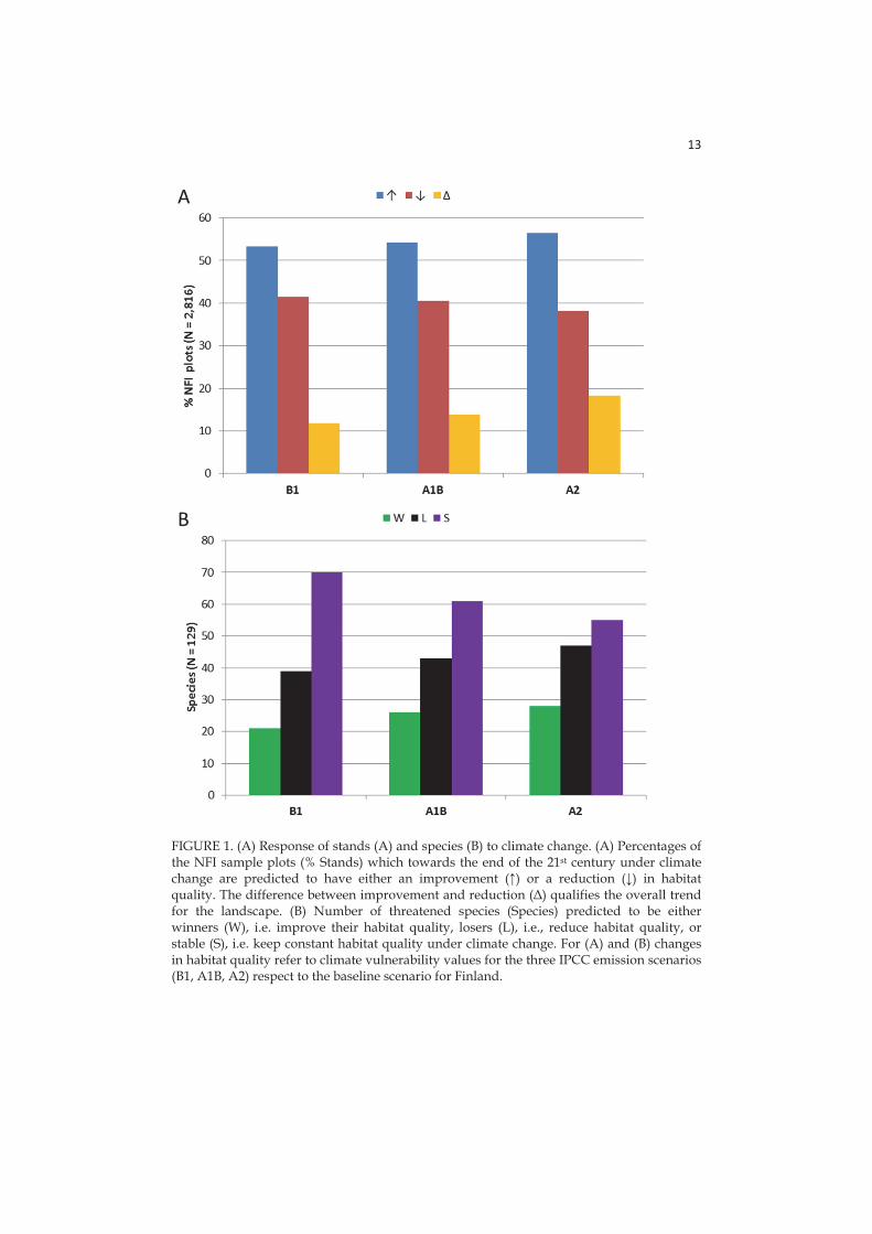
13

FIGURE 1. (A) Response of stands (A) and species (B) to climate change. (A) Percentages of the NFI sample plots (% Stands) which towards the end of the 21st century under climate change are predicted to have either an improvement ( ) or a reduction ( ) in habitat quality. The difference between improvement and reduction ( ) qualifies the overall trend for the landscape. (B) Number of threatened species (Species) predicted to be either winners (W), i.e. improve their habitat quality, losers (L), i.e., reduce habitat quality, or stable (S), i.e. keep constant habitat quality under climate change. For (A) and (B) changes in habitat quality refer to climate vulnerability values for the three IPCC emission scenarios (B1, A1B, A2) respect to the baseline scenario for Finland.

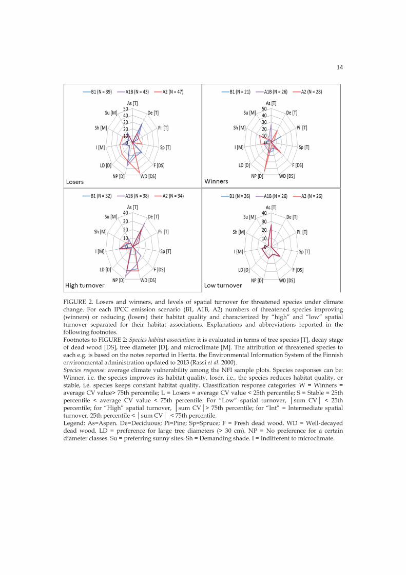
14

FIGURE 2. Losers and winners, and levels of spatial turnover for threatened species under climate change. For each IPCC emission scenario (B1, A1B, A2) numbers of threatened species improving (winners) or reducing (losers) their habitat quality and characterized by “high” and “low” spatial turnover separated for their habitat associations. Explanations and abbreviations reported in the following footnotes. Footnotes to FIGURE 2: Species habitat association: it is evaluated in terms of tree species [T], decay stage of dead wood [DS], tree diameter [D], and microclimate [M]. The attribution of threatened species to each e.g. is based on the notes reported in Hertta. the Environmental Information System of the Finnish environmental administration updated to 2013 (Rassi et al. 2000). Species response: average climate vulnerability among the NFI sample plots. Species responses can be: Winner, i.e. the species improves its habitat quality, loser, i.e., the species reduces habitat quality, or stable, i.e. species keeps constant habitat quality. Classification response categories: W = Winners = average CV value> 75th percentile; L = Losers = average CV value < 25th percentile; S = Stable = 25th percentile < average CV value < 75th percentile. For “Low“ spatial turnover, sum CV < 25th percentile; for “High” spatial turnover, sum CV > 75th percentile; for “Int” = Intermediate spatial turnover, 25th percentile < sum CV < 75th percentile. Legend: As=Aspen. De=Deciduous; Pi=Pine; Sp=Spruce; F = Fresh dead wood. WD = Well-decayed dead wood. LD = preference for large tree diameters (> 30 cm). NP = No preference for a certain diameter classes. Su = preferring sunny sites. Sh = Demanding shade. I = Indifferent to microclimate.

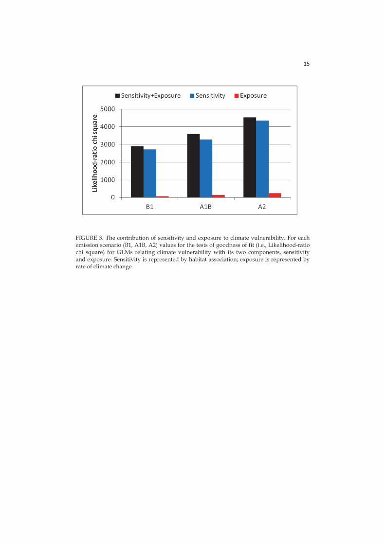
15

FIGURE 3. The contribution of sensitivity and exposure to climate vulnerability. For each emission scenario (B1, A1B, A2) values for the tests of goodness of fit (i.e., Likelihood-ratio chi square) for GLMs relating climate vulnerability with its two components, sensitivity and exposure. Sensitivity is represented by habitat association; exposure is represented by rate of climate change.

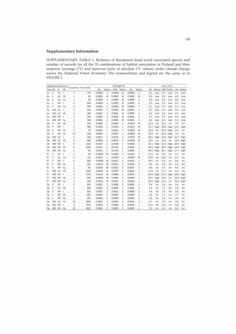
16

Supplementary Information

SUPPLEMENTARY TABLE 1. Richness of threatened dead wood associated species and number of records for all the 35 combinations of habitat association in Finland and their response (average CV) and turnover (sum of absolute CV values) under climate change across the National Forest Inventory The nomenclature and legend are the same as in FIGURE 2.

Tree DS D M B1 Status A1B Status A2 Status B1 Status A1B Status A2 StatusAs F LD I 5 774 0.0000 S 0.0000 W 0.0000 S 0.1 Low 0.1 Low 0.1 LowAs F LD Sh 1 63 0.0000 W 0.0000 W 0.0000 W 0.0 Low 0.0 Low 0.0 LowAs F LD Su 1 64 0.0000 S 0.0000 W 0.0000 S 0.0 Low 0.0 Low 0.0 LowAs F NP I 4 444 0.0000 S 0.0000 W 0.0000 S 0.1 Low 0.1 Low 0.1 LowAs F NP Su 6 494 0.0000 S 0.0000 W 0.0000 S 0.1 Low 0.1 Low 0.1 LowAs WD LD I 2 114 0.0002 S 0.0002 W 0.0001 S 0.5 Low 0.5 Low 0.4 LowAs WD LD Sh 3 760 0.0001 S 0.0001 W 0.0000 S 0.2 Low 0.2 Low 0.2 LowAs WD NP I 3 259 0.0002 S 0.0002 W 0.0001 S 0.7 Low 0.7 Low 0.5 LowAs WD NP Su 1 338 0.0001 S 0.0001 W 0.0001 S 0.4 Low 0.4 Low 0.3 LowDe F LD Sh 1 331 0.0039 L 0.0043 S 0.0013 W 15.3 Int 15.1 Int 7.0 IntDe F NP I 4 468 0.0100 L 0.0109 L 0.0017 W 37.2 High 36.8 High 12.5 HighDe F NP Sh 1 79 0.0051 L 0.0055 L 0.0016 W 19.4 Int 19.3 High 8.3 IntDe F NP Su 10 920 0.0066 L 0.0072 L 0.0004 W 23.5 Int 23.2 High 7.0 IntDe WD LD I 1 244 0.0017 S 0.0032 S 0.0070 W 26.6 High 23.8 High 21.7 HighDe WD LD Sh 3 966 0.0006 S 0.0013 S 0.0038 W 12.6 Int 11.4 Int 12.0 HighDe WD NP I 9 1120 0.0129 L 0.0148 L 0.0036 L 51.1 High 51.0 High 20.0 HighDe WD NP Sh 6 1456 0.0101 L 0.0114 L 0.0016 L 39.3 High 39.0 High 14.8 HighDe WD NP Su 1 87 0.0130 L 0.0145 L 0.0044 L 45.0 High 45.7 High 17.7 HighPi F LD I 1 56 0.0028 W 0.0018 S 0.0010 S 11.5 Int 6.0 Int 5.1 IntPi F LD Su 6 725 0.0051 L 0.0056 L 0.0003 W 18.6 Int 18.3 Int 6.2 IntPi F NP I 4 563 0.0048 W 0.0027 S 0.0016 S 18.5 Int 9.3 Int 8.0 IntPi F NP Sh 1 361 0.0023 W 0.0015 S 0.0010 S 9.5 Int 5.0 Int 4.3 IntPi F NP Su 1 93 0.0023 W 0.0013 S 0.0007 S 9.0 Int 4.7 Int 4.0 IntPi WD LD Sh 3 1020 0.0043 W 0.0037 S 0.0035 L 17.9 Int 11.7 Int 11.5 IntPi WD NP I 5 1710 0.0135 W 0.0082 L 0.0075 L 48.9 High 27.4 High 26.9 HighPi WD NP Sh 2 691 0.0063 W 0.0046 S 0.0044 L 24.5 High 15.0 Int 14.8 HighPi WD NP Su 3 530 0.0071 W 0.0047 S 0.0043 L 25.9 High 15.5 Int 15.4 HighSp F LD I 2 455 0.0005 S 0.0008 S 0.0005 S 2.6 Int 2.4 Int 1.9 IntSp F LD Sh 2 268 0.0002 S 0.0004 S 0.0002 S 1.4 Int 1.2 Int 1.0 IntSp F NP I 3 565 0.0007 S 0.0012 S 0.0008 S 4.0 Int 3.5 Int 3.0 IntSp F NP Sh 4 892 0.0004 S 0.0007 S 0.0005 S 2.4 Int 2.1 Int 1.7 IntSp F NP Su 2 205 0.0006 S 0.0009 S 0.0005 S 2.6 Int 2.5 Int 1.9 IntSp WD LD Sh 10 2936 0.0002 S 0.0014 S 0.0013 S 4.7 Int 4.3 Int 3.8 IntSp WD NP I 5 1541 0.0004 S 0.0040 S 0.0036 L 13.3 Int 11.6 Int 11.0 IntSp WD NP Sh 13 3923 0.0002 S 0.0022 S 0.0020 L 7.3 Int 6.5 Int 5.9 Int

Sum CVN.species N.recordsAverage CVHabitat Preferences

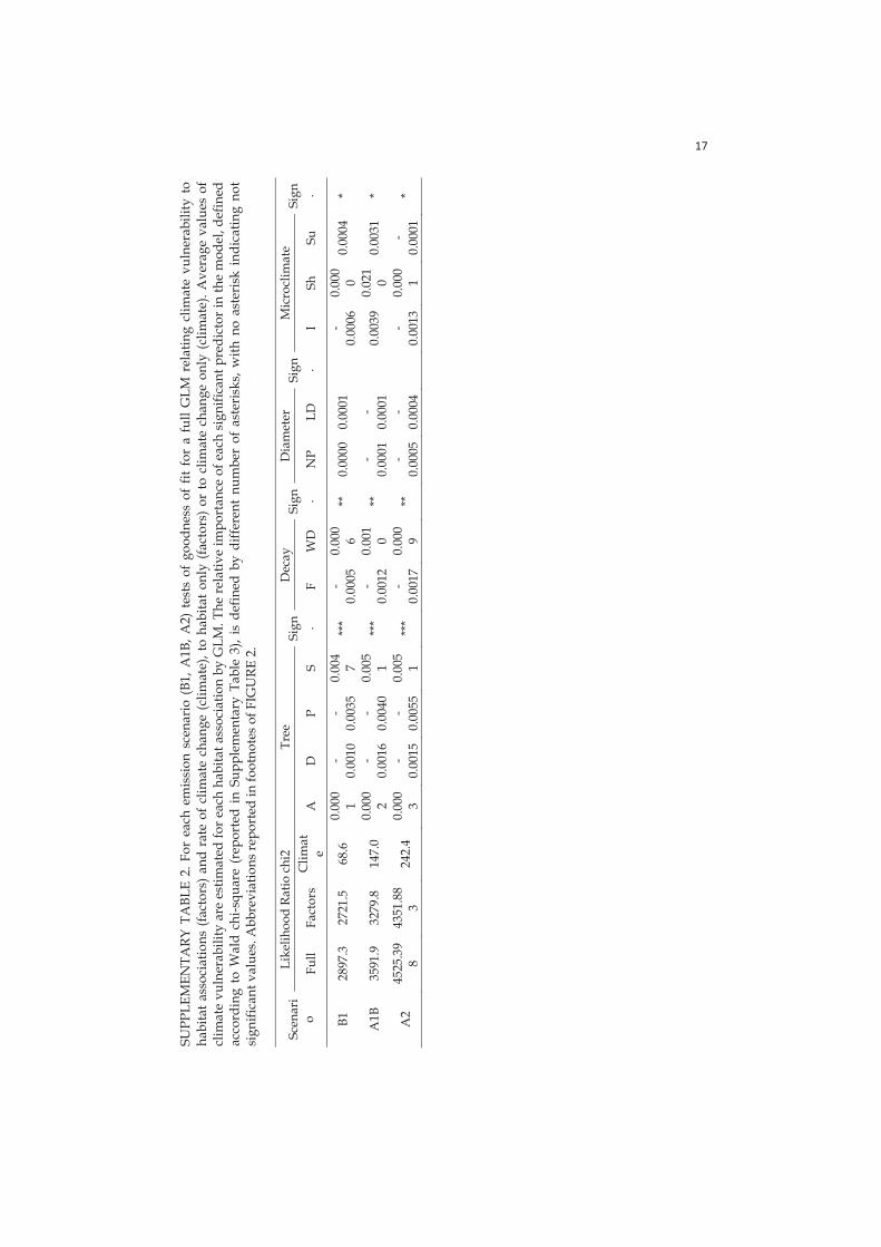
SUPP

LEM

ENTA

RY T

ABL

E 2.

For

eac

h em

issi

on s

cena

rio

(B1,

A1B

, A2)

tes

ts o

f go

odne

ss o

f fit

for

a f

ull G

LM r

elat

ing

clim

ate

vuln

erab

ility

to

habi

tat a

ssoc

iatio

ns (

fact

ors)

and

rat

e of

clim

ate

chan

ge (

clim

ate)

, to

habi

tat o

nly

(fact

ors)

or

to c

limat

e ch

ange

onl

y (c

limat

e). A

vera

ge v

alue

s of

cl

imat

e vu

lner

abili

ty a

re e

stim

ated

for e

ach

habi

tat a

ssoc

iatio

n by

GLM

. The

rela

tive

impo

rtan

ce o

f eac

h si

gnifi

cant

pre

dict

or in

the

mod

el, d

efin

ed

acco

rdin

g to

Wal

d ch

i-squ

are

(rep

orte

d in

Sup

plem

enta

ry T

able

3),

is d

efin

ed b

y di

ffere

nt n

umbe

r of

ast

eris

ks, w

ith n

o as

teri

sk i

ndic

atin

g no

t si

gnifi

cant

val

ues.

Abb

revi

atio

ns re

port

ed in

foot

note

s of

FIG

URE

2.

Scen

ari

o

Like

lihoo

d Ra

tio c

hi2

Tree

Si

gn .

Dec

ay

Sign .

Dia

met

er

Sign .

Mic

rocl

imat

e Si

gn . Fu

ll Fa

ctor

s C

limat

e A

D

P

S F

WD

N

P LD

I

Sh

Su

B1

2897

.3

2721

.5

68.6

0.

000

1 -

0.00

10

-0.

0035

0.

004

7 **

* -

0 .00

05

0.00

06

**

0.00

00

0.00

01

-

0.00

06

0.00

00

0 .00

04

*

A1B

35

91.9

32

79.8

14

7.0

0.00

02

-0.

0016

-

0.00

40

0.00

51

***

-0 .

0012

0.

001

0 **

-

0.00

01

-0.

0001

0.00

39

0.02

10

0 .00

31

*

A2

4525

.39

8 43

51.8

83

242.

4 0.

000

3 -

0.00

15

-0.

0055

0.

005

1 **

* -

0 .00

17

0.00

09

**

-0.

0005

-

0.00

04

-

0.00

13

0.00

01

-0 .

0001

*

17

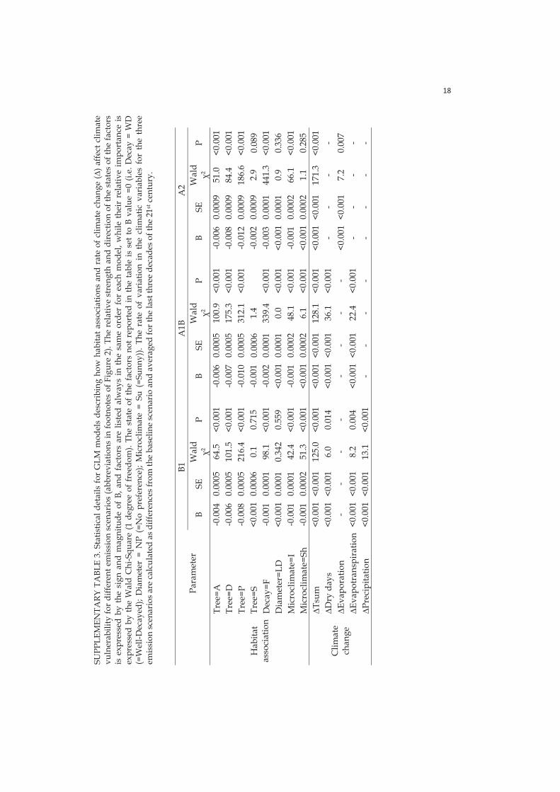
SUPP

LEM

ENTA

RY T

ABL

E 3.

Sta

tistic

al d

etai

ls fo

r G

LM m

odel

s de

scri

bing

how

hab

itat a

ssoc

iatio

ns a

nd r

ate

of c

limat

e ch

ange

() a

ffect

clim

ate

vuln

erab

ility

for

diffe

rent

em

issi

on s

cena

rios

(abb

revi

atio

ns in

foot

note

s of

Fig

ure

2). T

he r

elat

ive

stre

ngth

and

dir

ectio

n of

the

stat

es o

f the

fact

ors

is e

xpre

ssed

by

the

sign

and

mag

nitu

de o

f B,

and

fac

tors

are

list

ed a

lway

s in

the

sam

e or

der

for

each

mod

el, w

hile

the

ir r

elat

ive

impo

rtan

ce is

ex

pres

sed

by th

e W

ald

Chi

-Squ

are

(1 d

egre

e of

fre

edom

). Th

e st

ate

of th

e fa

ctor

s no

t rep

orte

d in

the

tabl

e is

set

to B

val

ue =

0 (i.

e. D

ecay

= W

D

(=W

ell-D

ecay

ed);

Dia

met

er =

NP

(=N

o pr

efer

ence

); M

icro

clim

ate

= Su

(=S

unny

)). T

he r

ate

of v

aria

tion

in t

he c

limat

ic v

aria

bles

for

the

thr

ee

emis

sion

sce

nari

os a

re c

alcu

late

d as

diff

eren

ces

from

the

base

line

scen

ario

and

ave

rage

d fo

r the

last

thre

e de

cade

s of t

he 2

1st c

entu

ry.

Pa

ram

eter

B1

A1B

A2

B SE

W

ald ²

P

B SE

W

ald ²

P

B SE

W

ald ²

P

Hab

itat

asso

ciat

ion

Tree

=A

-0.0

04

0.00

05

64.5

<0

.001

-0.0

06

0.00

05

100.

9 <0

.001

-0.0

06

0.00

09

51.0

<0

.001

Tr

ee=D

-0

.006

0.

0005

10

1.5

<0.0

01

-0

.007

0.

0005

17

5.3

<0.0

01

-0

.008

0.

0009

84

.4

<0.0

01

Tree

=P

-0.0

08

0.00

05

216.

4 <0

.001

-0.0

10

0.00

05

312.

1 <0

.001

-0.0

12

0.00

09

186.

6 <0

.001

Tr

ee=S

<0

.001

0.

0006

0.

1 0.

715

-0.0

01

0.00

06

1.4

-0.0

02

0.00

09

2.9

0.08

9 D

ecay

=F

-0.0

01

0.00

01

98.1

<0

.001

-0.0

02

0.00

01

339.

4 <0

.001

-0.0

03

0.00

01

441.

3 <0

.001

D

iam

eter

=LD

<0

.001

0.

0001

0.

342

0.55

9

<0.0

01

0.00

01

0.0

<0.0

01

<0

.001

0.

0001

0.

9 0.

336

Mic

rocl

imat

e=I

-0.0

01

0.00

01

42.4

<0

.001

-0.0

01

0.00

02

48.1

<0

.001

-0.0

01

0.00

02

66.1

<0

.001

M

icro

clim

ate=

Sh

-0.0

01

0.00

02

51.3

<0

.001

<0.0

01

0.00

02

6.1

<0.0

01

<0

.001

0.

0002

1.

1 0.

285

Clim

ate

chan

ge

Tsum

<0

.001

<0.

001

125.

0 <0

.001

<0.0

01 <

0.00

1 12

8.1

<0.0

01

<0

.001

<0.

001

171.

3 <0

.001

D

ry d

ays

<0.0

01 <

0.00

1 6.

0 0.

014

<0

.001

<0.

001

36.1

<0

.001

- -

- -

Evap

orat

ion

- -

- -

- -

- -

<0.0

01 <

0.00

1 7.

2 0.

007

Evap

otra

nspi

ratio

n <0

.001

<0.

001

8.2

0.00

4

<0.0

01 <

0.00

1 22

.4

<0.0

01

-

- -

- Pr

ecip

itati o

n <0

.001

<0.

001

13.1

<0

.001

- -

- -

-

- -

-

18

III APPLYING A FRAMEWORK FOR LANDSCAPE PLANNING UNDER CLIMATE CHANGE FOR THE CONSERVATION OF

BIODIVERSITY IN THE FINNISH BOREAL FOREST

by

Adriano Mazziotta, Maria Triviño, Olli-Pekka Tikkanen, Jari Kouki,

Harri Strandman & Mikko Mönkkönen

Global Change Biology doi: 10.1111/gcb.12677

Reprinted with kind permission of

© John Wiley & Sons, Inc.

IV

OPTIMAL CONSERVATION RESOURCE ALLOCATION UNDER VARIABLE ECONOMIC AND ECOLOGICAL TIME

DISCOUNTING RATES IN BOREAL FOREST

by

Adriano Mazziotta, Federico Montesino Pouzols, Mikko Mönkkönen, Janne S. Kotiaho, Harri Strandman & Atte Moilanen

Submitted manuscript

1

OPTIMAL CONSERVATION RESOURCE ALLOCATION

UNDER VARIABLE ECONOMIC AND ECOLOGICAL TIME

DISCOUNTING RATES IN BOREAL FOREST

Adriano Mazziotta1,*, Federico M. Pouzols2,*, Mikko Mönkkönen1, Janne S.

Kotiaho1, Harri Strandman3 and Atte Moilanen2

*Equal first authors

1Department of Biological and Environmental Science, P.O. Box 35, 40014

University of Jyväskylä, Finland 2Department of Biosciences, P.O. Box 65, 00014 University of Helsinki, Finland 3School of Forest Sciences, P.O. Box 111, University of Eastern Finland, 80101

Joensuu, Finland

Corresponding author: Federico M. Pouzols,

federico.montesinopouzols@helsinki.fi, Finnish Centre of Excellence in

Metapopulation Biology, Department of Biosciences, P.O. Box 65, University of

Helsinki, FI-00014, Finland. Phone: +358-09-19157714

Running head: Ecological and economical time discounting

Keywords: clear-cut; complementarity; conservation planning; forest

management; forest simulator; habitat restoration; RobOff software; time

discounting

Word count: 5,789 words.

Type of article: Contributed paper

2

Abstract

Resource allocation to multiple alternative conservation actions is a complex task. A common trade-off occurs between protection of smaller, expensive, high-quality areas versus larger, cheaper, partially degraded areas. Here, we investigate optimal allocation into three actions in boreal forest: current standard forest management rules (business-as-usual), setting aside of mature stands, or setting aside of clear-cuts. We first estimated how habitat availability for focal indicator species and economic returns from timber harvesting develop through time as a function of forest type and action chosen. We then developed an optimal resource allocation by accounting for budget size and habitat availability of indicator species in different forest types. We also accounted for the perspective adopted towards sustainability, modeled via temporal preference and economic and ecological time discounting. Controversially, we found that in boreal forest set-aside followed by protection of clear-cuts can become a winning cost-effective strategy when accounting for habitat requirements of multiple species, a long planning horizon, and a limited budget. It is particularly effective when adopting a long-term sustainability perspective, and accounting for present revenues from timber harvesting. More generally, the present work demonstrates an analysis by which it is possible to assess the cost-effective conditions to allocate resources into an inexpensive - and possibly controversial - conservation strategy that nevertheless has potential to produce high ecological values in the future.

3

Introduction

In a world dominated by human impacts, where habitat degradation is reducing the space suitable for species, there are different alternatives to protect land when economical resources are limited (Polasky et al. 2008, Mönkkönen et al. 2011). Given the importance of habitat area and quality in conservation (Hodgson et al. 2011), taking two extremes, we can set-aside small selected areas of high quality habitats or we can set-aside as much area as we can, caring less for quality. In the former case we usually assume high habitat quality for species in these selected core areas; in the latter case we create a bigger reserve network that may compensate lower average habitat quality by increased area. Conceptually for boreal forest, setting aside large areas of presently lower quality habitat can be a long-term winning strategy, for at least three reasons (J. S. K. and M. M. unpublished data). First, those areas will follow natural succession and improve in their quality through time. Second, the economic effort required to set aside this network may be much lower, thereby reducing conflict with stakeholders. This is assuming that lower habitat quality is correlated with lower economic value, as is the case specifically for the boreal forests in Fennoscandia that are focus of this study (Mönkkönen et al. 2014). Finally, choosing a few sites of high habitat quality (and high cost) can result in lower than expected long-term benefits: areas can be damaged by natural or human disturbance; a small protected area is likely to be unable to maintain spatial population dynamics leading to delayed extinctions via the extinction debt (Kuussaari et al. 2009). As a contrary argument, many species simply cannot survive outside high-quality late successional habitats, implying that such habitats must be included in any successful conservation area network (e.g., Hodgson et al. 2009, Mönkkönen et al. 2011).

In favor of protecting large conservation area networks is the species-area relationship, which states that there is a positive relationship between the area of a site and the number of species found on it. This relationship is one of the most general patterns observed in ecology (Rosenzweig 1995). On the other hand, empirical observations show that species extinctions follow habitat loss, although often with a considerable time lag (Kuussaari et al. 2009). This implies that a conservation strategy opting for good quality habitats can maintain viable populations in the short term, but isolation and the small aggregate area of the sites could reduce the survival of populations in the long term. Both theory and practice suggest that successful conservation must aim at a balance between area and mean habitat quality (Hodgson et al. 2011).

Considering economics, the net present economic value of an area is combination of the revenue it can produce now and the time discounted revenue it could produce through time. Because future benefits are uncertain, future revenue is usually valued less than immediately available revenue. In contrast, the ecological value of the same area across time can be interpreted from different perspectives. From a utilitarian perspective, the area should have a higher ecological value at present, because the pleasure derived from the presence of biodiversity can only be fully appreciated at the present (Fuller et al.

4

2007). The conservation perspective assumes a higher ecological value to an area if it can ensure future persistence of species. These two perspectives base their rationale from alternative perceptions of nature as a balance or a flux (sensu Ladle and Gilson 2008). From the sustainability perspective, transmitting ecological values to future generations is the key (Child 2011).

The choice of the planning horizon or time window for evaluating ecological benefits is a key issue for conservation. Both economic and ecological benefits are dynamic: the former depend on the time an area provides valuable goods; the latter depend on the time the area is suitable for species of interest. Both are mediated through time by biological processes and are conditional on management taken (or lack of it) in the area. Consequently, it becomes necessary to jointly investigate the economic and ecological value of an area through time. However, future benefits of conservation may not be discountable in the same way as are economic values (Gollier 2010, Kula and Evans 2011, Guéant et al. 2012). Based on a logical scrutiny of economic discounting, Philibert (2003) argued that irreplaceable and non-reproducible environmental assets should be given a value growing over time at a pace close to the economic discount rate. A high net present value of future environmental benefits justifies increased immediate investment into conservation (Philibert 2003). Long time spans (centuries) are justified in the evaluation of conservation benefits and ecological values, because these benefits are produced by functioning ecosystems and ecological processes and structures that take a long time to establish but can be lost very quickly due to human disturbance.

In Fennoscandia, intensive timber extraction has led to decline of forest biodiversity, and there is a recognized need to expand forest conservation (Brumelis et al. 2011). Here, we investigate optimal allocation of resources between three alternative actions in boreal forests. First, our baseline is business-as-usual commercial forest management. Our second alternative is typical forest conservation enacted via setting aside of mature stands, which offers relatively high immediate ecological quality but with high per-area cost. The third alternative is setting aside of much larger areas of clear-cuts, which presently hold low economic and ecological value. Per-area costs of protecting clear-cuts are much lower than that of mature stands. The question becomes, can clear-cuts support enough ecological value through time to make them a viable complement for mature stands? While clear-cuts currently host few structures of biodiversity importance (Lundström et al. 2011), they can provide habitats for many species if they are allowed to develop via natural succession, including natural accumulation of dead wood (e.g. Junninen et al. 2006, Eräjää et al. 2010, Rudolphi and Gustafsson 2011, Swanson et al. 2011). They can even host an equal or greater number of species than old-growth forests (e.g. Pykälä 2004, Selonen et al. 2005).

The analysis done here was implemented using recently released software intended for the investigation of uncertain consequences of alternative (conservation) actions in different environments through time (Pouzols and Moilanen 2013). A structurally similar analysis could be replicated for other areas or environments with different environmental response functions.

5

Methods

Outline

We first used a stochastic forest growth simulator (SIMA, Kellomäki et al. 1992) to simulate forest growth in three different habitat types under different management scenarios. From the simulated stands we estimated how economic returns from timber harvesting and habitat suitability indexes (HSI) for six focal species develop over three centuries. Time discounted economic and ecological returns were used to produce response functions that are basic building blocks of the next step, optimal cost-effective allocation of alternative actions using the RobOff framework and software (Pouzols et al. 2012, Pouzols and Moilanen 2013). This analysis integrates species-specific responses to actions in different environments, uncertainty around these responses, costs of actions, availability of habitats suitable for different actions, and economical and ecological time discounting.

We compared three alternative management scenarios, Business-As-Usual (BAU), set-aside and protect as mature stand (SA), and clear-cut following set-aside and protect (CC+SA). By mature stands we do not mean mature old growth forests but commercially managed forests that have reached the mean diameter allowing clear cut. In Fennoscandia, mature old-growth-forests are available for conservation in very small areas only, and all of them naturally are first priority for conservation. In BAU, stands are managed according to the current widespread standard management recommendations. Since BAU has been developed for the needs of commercial forestry, we can assume that it produces long-term revenue that is economically optimal. BAU represents a baseline for our primary comparison, which is between SA and CC+SA. In both set-aside scenarios (SA and CC+SA), natural succession was assumed to follow; in CC+SA after the forest first has been cleared during the first 30 years. Our chosen time frame, 300 years, corresponds to about four rotations. Even if stands managed with CC+SA scenario may be of low ecological quality in the beginning they will quickly improve in quality through time. Details of management practices are provided in appendix S1.

Study areas

We randomly chose for the parameterization of response functions 553 mature stands from the data of the 9th National Forest Inventory (NFI, 1996-2003) (Finnish Forest Research Institute 2010). These stands are sampling plots of 100 m2 distributed across southern Finland on c. 7 million privately-owned forest hectares (30.8% of the forested area in Finland). Each stand has been classified to one of the three main forest site types in southern Finland based on the ground vegetation of the site (Cajander 1949). The site types are, in increasing fertility and water content (and by implication increasing productivity and land price), VT (Vaccinium Type; 57 stands), MT (Myrtillus Type; 301 stands), and OMT (Oxalis-Myrtillus Type; 195 stands). Silver birch and Norway spruce only occur naturally in OMT and MT sites but Scots pine also grows in the less fertile

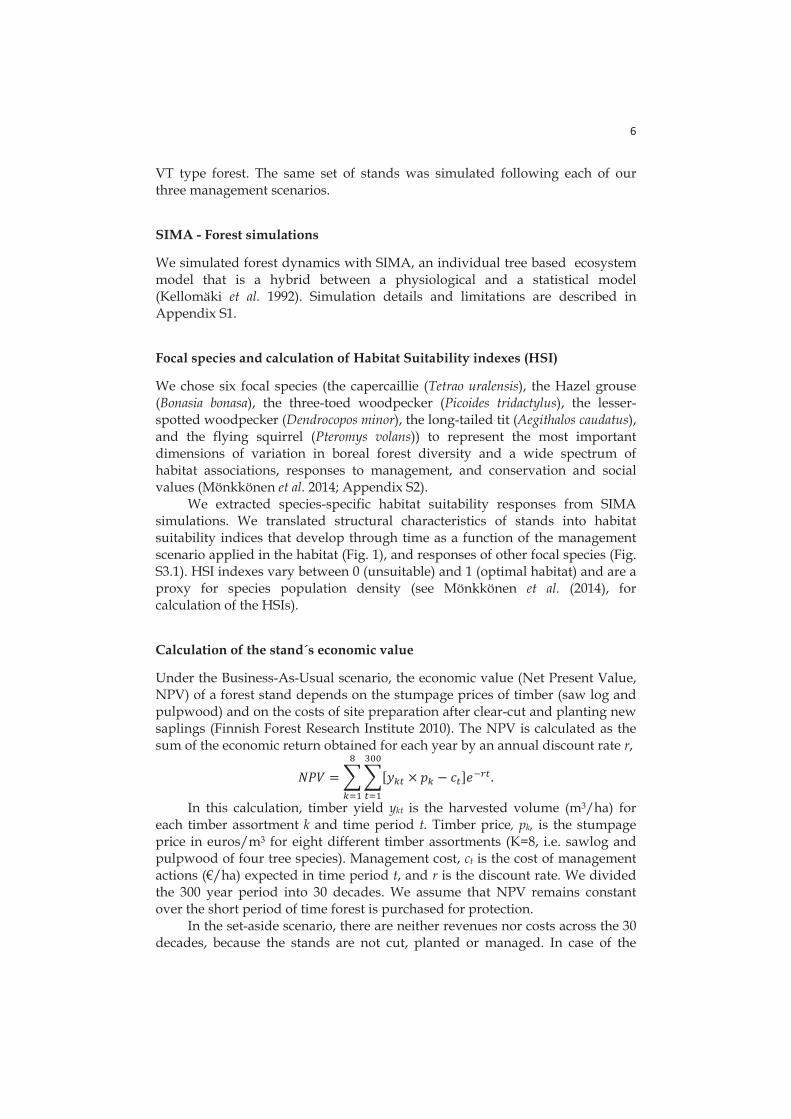
6

VT type forest. The same set of stands was simulated following each of our three management scenarios.

SIMA - Forest simulations

We simulated forest dynamics with SIMA, an individual tree based ecosystem model that is a hybrid between a physiological and a statistical model (Kellomäki et al. 1992). Simulation details and limitations are described in Appendix S1.

Focal species and calculation of Habitat Suitability indexes (HSI)

We chose six focal species (the capercaillie (Tetrao uralensis), the Hazel grouse (Bonasia bonasa), the three-toed woodpecker (Picoides tridactylus), the lesser-spotted woodpecker (Dendrocopos minor), the long-tailed tit (Aegithalos caudatus), and the flying squirrel (Pteromys volans)) to represent the most important dimensions of variation in boreal forest diversity and a wide spectrum of habitat associations, responses to management, and conservation and social values (Mönkkönen et al. 2014; Appendix S2).

We extracted species-specific habitat suitability responses from SIMA simulations. We translated structural characteristics of stands into habitat suitability indices that develop through time as a function of the management scenario applied in the habitat (Fig. 1), and responses of other focal species (Fig. S3.1). HSI indexes vary between 0 (unsuitable) and 1 (optimal habitat) and are a proxy for species population density (see Mönkkönen et al. (2014), for calculation of the HSIs).

Calculation of the stand´s economic value

Under the Business-As-Usual scenario, the economic value (Net Present Value, NPV) of a forest stand depends on the stumpage prices of timber (saw log and pulpwood) and on the costs of site preparation after clear-cut and planting new saplings (Finnish Forest Research Institute 2010). The NPV is calculated as the sum of the economic return obtained for each year by an annual discount rate r,

In this calculation, timber yield ykt is the harvested volume (m3/ha) for each timber assortment k and time period t. Timber price, pk, is the stumpage price in euros/m3 for eight different timber assortments (K=8, i.e. sawlog and pulpwood of four tree species). Management cost, ct is the cost of management actions (€/ha) expected in time period t, and r is the discount rate. We divided the 300 year period into 30 decades. We assume that NPV remains constant over the short period of time forest is purchased for protection.

In the set-aside scenario, there are neither revenues nor costs across the 30 decades, because the stands are not cut, planted or managed. In case of the

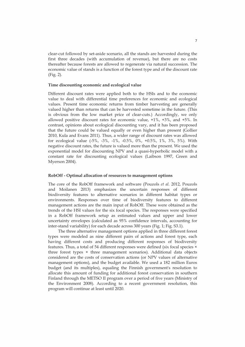
7

clear-cut followed by set-aside scenario, all the stands are harvested during the first three decades (with accumulation of revenue), but there are no costs thereafter because forests are allowed to regenerate via natural succession. The economic value of stands is a function of the forest type and of the discount rate (Fig. 2).

Time discounting economic and ecological value

Different discount rates were applied both to the HSIs and to the economic value to deal with differential time preferences for economic and ecological values. Present time economic returns from timber harvesting are generally valued higher than returns that can be harvested sometime in the future. (This is obvious from the low market price of clear-cuts.) Accordingly, we only allowed positive discount rates for economic value, +1%, +3%, and +5%. In contrast, opinions about ecological discounting vary, and it has been proposed that the future could be valued equally or even higher than present (Gollier 2010, Kula and Evans 2011). Thus, a wider range of discount rates was allowed for ecological value (-5%, -3%, -1%, -0.5%, 0%, +0.5%, 1%, 3%, 5%). With negative discount rates, the future is valued more than the present. We used the exponential model for discounting NPV and a quasi-hyperbolic model with a constant rate for discounting ecological values (Laibson 1997, Green and Myerson 2004).

RobOff - Optimal allocation of resources to management options

The core of the RobOff framework and software (Pouzols et al. 2012, Pouzols and Moilanen 2013) emphasizes the uncertain responses of different biodiversity features to alternative scenarios in different habitat types or environments. Responses over time of biodiversity features to different management actions are the main input of RobOff. These were obtained as the trends of the HSI values for the six focal species. The responses were specified in a RobOff framework setup as estimated values and upper and lower uncertainty envelopes (calculated as 95% confidence intervals, accounting for inter-stand variability) for each decade across 300 years (Fig. 1; Fig. S3.1).

The three alternative management options applied in three different forest types were modeled as nine different pairs of actions and forest type, each having different costs and producing different responses of biodiversity features. Thus, a total of 54 different responses were defined (six focal species × three forest types × three management scenarios). Additional data objects considered are the costs of conservation actions (or NPV values of alternative management options), and the budget available. We used a 182 million Euros budget (and its multiples), equaling the Finnish government's resolution to allocate this amount of funding for additional forest conservation in southern Finland through the METSO II program over a period of five years (Ministry of the Environment 2008). According to a recent government resolution, this program will continue at least until 2020.

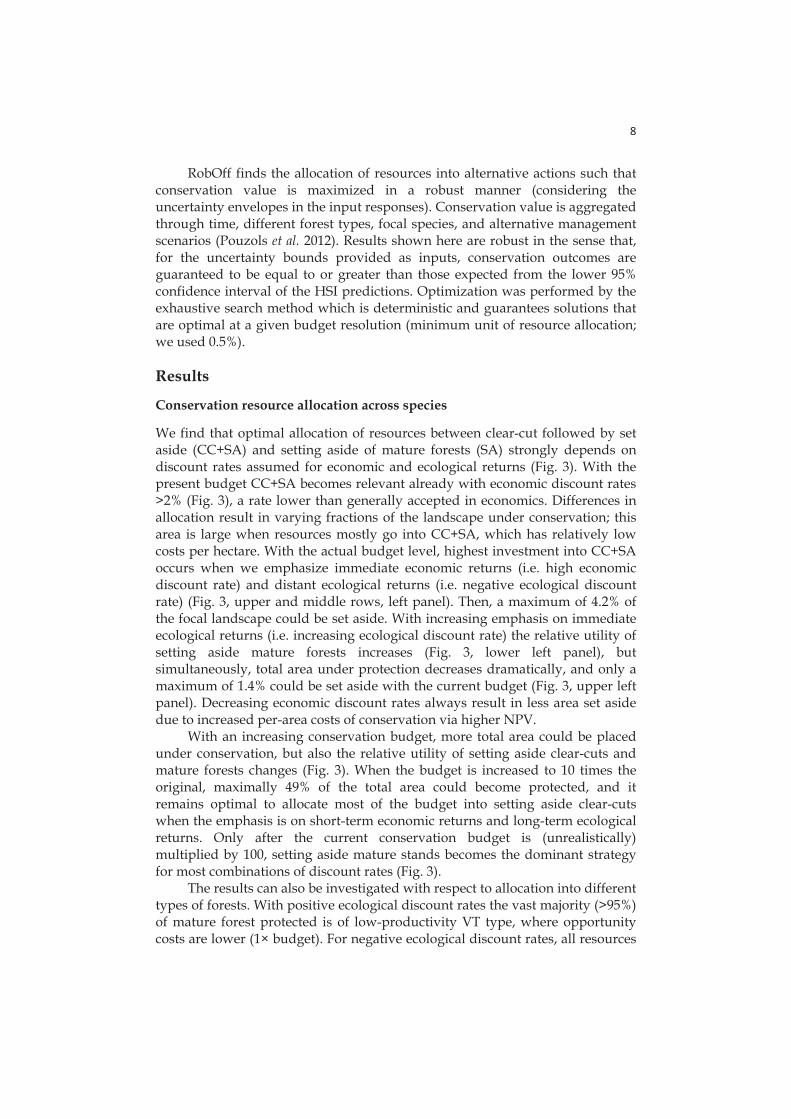
8

RobOff finds the allocation of resources into alternative actions such that conservation value is maximized in a robust manner (considering the uncertainty envelopes in the input responses). Conservation value is aggregated through time, different forest types, focal species, and alternative management scenarios (Pouzols et al. 2012). Results shown here are robust in the sense that, for the uncertainty bounds provided as inputs, conservation outcomes are guaranteed to be equal to or greater than those expected from the lower 95% confidence interval of the HSI predictions. Optimization was performed by the exhaustive search method which is deterministic and guarantees solutions that are optimal at a given budget resolution (minimum unit of resource allocation; we used 0.5%).

Results

Conservation resource allocation across species

We find that optimal allocation of resources between clear-cut followed by set aside (CC+SA) and setting aside of mature forests (SA) strongly depends on discount rates assumed for economic and ecological returns (Fig. 3). With the present budget CC+SA becomes relevant already with economic discount rates >2% (Fig. 3), a rate lower than generally accepted in economics. Differences in allocation result in varying fractions of the landscape under conservation; this area is large when resources mostly go into CC+SA, which has relatively low costs per hectare. With the actual budget level, highest investment into CC+SA occurs when we emphasize immediate economic returns (i.e. high economic discount rate) and distant ecological returns (i.e. negative ecological discount rate) (Fig. 3, upper and middle rows, left panel). Then, a maximum of 4.2% of the focal landscape could be set aside. With increasing emphasis on immediate ecological returns (i.e. increasing ecological discount rate) the relative utility of setting aside mature forests increases (Fig. 3, lower left panel), but simultaneously, total area under protection decreases dramatically, and only a maximum of 1.4% could be set aside with the current budget (Fig. 3, upper left panel). Decreasing economic discount rates always result in less area set aside due to increased per-area costs of conservation via higher NPV.

With an increasing conservation budget, more total area could be placed under conservation, but also the relative utility of setting aside clear-cuts and mature forests changes (Fig. 3). When the budget is increased to 10 times the original, maximally 49% of the total area could become protected, and it remains optimal to allocate most of the budget into setting aside clear-cuts when the emphasis is on short-term economic returns and long-term ecological returns. Only after the current conservation budget is (unrealistically) multiplied by 100, setting aside mature stands becomes the dominant strategy for most combinations of discount rates (Fig. 3).

The results can also be investigated with respect to allocation into different types of forests. With positive ecological discount rates the vast majority (>95%) of mature forest protected is of low-productivity VT type, where opportunity costs are lower (1× budget). For negative ecological discount rates, all resources

9

would be allocated into medium-productivity MT type. On the other hand, for CC+SA most of the budget (>90%) is allocated into high-productivity OMT areas, except for very low ecological discount rates (-3 to -5%) in which case all resources go into MT areas. These results are explained by the different costs of action in different forest types and different delays in ecological responses. MT forests have a more favorable combination of long-term average conservation value and land/opportunity cost than other forest types.

Species specific conservation resource allocation

The relative utility of setting aside clear-cuts and mature forests varies significantly between the species, reflecting species-specific habitat requirements (Fig. 1; Fig. S3.1). We illustrate this variation by showing the optimal allocation for three species: the flying squirrel, for which set-aside of mature stands provided highest average HSI values; the capercaillie, for which there were no significant differences in HSI values between scenarios; and the long-tailed tit, for which CC+SA provides highest HSI values.

The largest total area becomes protected when the economic discount rate is high and the ecological discount rate is negative (Figs. 3 and 4). The relative utility of setting aside mature forests vs. clear-cuts varies markedly between species (Fig. 4). At the current budget level, setting aside clear-cut remains a part of the conservation tool-box for all species (Fig. 4). When the focal species has a strong association with mature forests (e.g., the flying squirrel) it is optimal to allocate only a low fraction of resources into clear-cuts (Fig. 4) and only under limited combinations of ecological and economic discounting. For other species, optimal allocation into CC+SA is overall higher (e.g. long-tailed tit) or takes place under a wider combination of discount rates (capercaillie).

Discussion

We have used the RobOff software to quantitatively investigate optimal conservation resource allocation in boreal forests in Finland. Our analysis showed that when a longer time perspective is adopted, unconventional decisions, such as allocating resources into an inexpensive conservation action (setting aside and protecting clear-cuts) that has potential to produce high ecological values in the future, may make sense. This is true in particular when the conservation budget is limited, present revenues from timber extraction are preferred, and, following guidelines of sustainability and intergenerational equity, both present and future ecological benefits are valued. Importantly, we note that we are not advocating for clear-cutting forestry, but in a context that is already about 98% dominated by intensive forestry with clear-cut final harvesting, allocating a proportion of conservation resources for protecting clear-cut areas would be a cost-efficient policy in the long-run. Consequently, the Finnish environmental administration (and neighboring countries) could consider setting aside a larger area of clear-cuts as a valid alternative to the purchase of old managed stands (Lundström et al. 2011). Note that only part of

10

the budget should be used for clear-cuts (Fig. 3), and that clear-cuts should be left alone to follow natural succession (Rudolphi and Gustafsson 2011, Swanson et al. 2011).

Our analyses also found differences between optimal allocations of resources into forests of different productivity. When mature stands are protected, the preference should be on low-productivity low-cost VT types, with lower cost per area, whereas with clear-cuts more productive forest land should be preferred (Lundström et al. 2011).

Current conservation investments in Finland are not enough for achieving the Aichi conservation targets, which require protection of at least 17% of terrestrial areas by 2020 (European Commission 2010). Presently, approximately 10% of the terrestrial areas of Finland belong to public and private protected areas, implying that a further 7% of the territory should additionally be protected, which in South-Finland converts into an expansion of about 483 000 ha of forest conservation areas. Therefore, the actual present forest conservation budget could achieve up to 59% of the Aichi target (about 282 900 ha) if used to set-aside clear-cuts, but only up to 20% of the Aichi target (about 96 600 ha) if setting aside only mature stands. According to the present analysis, the Aichi target would be achieved with a balance of mature stands and clear-cuts under a quota of approximately ten times the actual current forest conservation budget.

One factor strongly influencing decisions over long time periods is balancing of immediate versus distant gains and losses, which we implemented via time discounting (Green and Myerson 2004). We used separate time discounting for economic and ecological values inside RobOff. Arguments in favor of dual discounting are based on the fundamentally different characters of environmental benefits and monetary costs. At least three reasons have been proposed for the use of zero or even negative discount rates for ecological values: (i) partial non-substitutability of ecological and biodiversity values by economic growth/consumption, (ii) guaranteeing of intergenerational equity, and (iii) providing an adequate basis for long-term persistence of biodiversity (Gollier 2010, Kula and Evans 2011). The lower the growth rate of environmental quality (or the larger its rate of decline), and the lower the elasticity of substitution between environmental quality and produced goods, the lower the ecological discount rate should be (Hoel and Sterner 2008). Our results also show that setting aside clear-cuts becomes especially effective when the economic discount rate is >2%. It is not possible to find a single general discount rate for forestry investments but realistic rates have typically been >2% (e.g. Grege-Staltmane and Tuherm 2010, Finnish Forest Research Institute 2010). If we accept the widely held assumption that ecological discount rates should be well below the economic ones (Gollier 2010, Guéant et al. 2012), decision makers should apply ecological discount rates closer to zero or negative. The strategy of CC+SA indeed seems a viable option for a plausible range of time discount rates for economic and ecological benefits.

Some assumptions and choices were made to facilitate the present analysis. For example, because species have different responses it makes a

11

difference which ones are included in analysis (Fig. 4; Fig. S3.1). The six species included here are associated with mid-seral or late-seral forest stages, and as such are considered indicators of high-quality boreal forest (Mönkkönen et al. 2014). Nevertheless, a different choice towards early-seral species associated with young forests could lead to a different optimal resource allocation, which by necessity will be more biased towards setting aside of clear-cuts. Overall, the strategy of partial investment into clear-cuts seems a robust strategy: CC+SA produces habitats that support many species in the long run and large areas could be afforded. Indeed the long-term benefits of CC+SA in terms of HSI are as highly certain as the favorable short-term responses from SA, conditional on natural succession been allowed through the establishment of permanent reserves (Mönkkönen et al. 2011).

A simplification of the present analysis is that RobOff does not account for spatial patterns, which however is not a major impediment for the applicability of the results. Survival of species obviously depends on the overall structure of the landscape. Once we have identified the relevance of setting-aside clear-cuts, it is a simple matter to purchase these from the neighborhood of the remaining old-growth forests, almost all of which already are under protection. Thus, it is possible to ensure adequate connectivity and colonization potential. Also, all our focal taxa are vertebrates capable of long-distance dispersal and recolonization of empty habitat. Making the present analysis fully spatial would on the other hand be highly expensive in terms of data and computational demands. As another limitation, our analysis only considered two strategies (BAU and SA) widely applied in Fennoscandian boreal forests. Alternative strategies have recently been suggested, such as selective logging (Hjälten et al. 2012), partial harvesting (Thorpe et al. 2010), or uneven-aged management (Kuuluvainen et al. 2012) but little is currently known about their effects on biodiversity. Subsequent improved analysis could also include additional focal guilds, such as forest dwelling beetles and polypore fungi, which have well-known habitat requirements (Tikkanen et al. 2006), and whose occurrence is related to forest management (Siitonen 2001, Mönkkönen et al. 2011).

While the present analysis focuses on and is highly relevant for boreal forests in Finland, and by extrapolation in the neighboring areas of Fennoscandia, the insights gained could be extrapolated to different environments with similar relationships between opportunity costs and environmental responses. We anticipate that setting aside forests where timber has been extracted can be a part of a long-term conservation tool-box in all forest biomes where the total area of forests is not diminishing but a large proportion of area is under human influence. We do not recommend applying this strategy in less resilient ecosystems where natural succession is not likely to restore ecological values or in ecosystems where remaining natural areas are declining rapidly. In such cases it would be unrealistic to assume that species would persist until degraded areas regain their suitability via natural succession.

The present multi-dimensional analysis summarizes effects of alternative conservation actions on the occurrence of priority fauna in different types of

12

boreal forests through time. It is among the first major studies that integrate both economic and ecological discounting in conservation resource allocation. We quantitatively identified sets of actions that produce high conservation value that is balanced across features, forest environments and time, guided by costs and budget availability. Our results suggest that protection of clear-cuts preferably nearby existing high-quality forest conservation areas would be a feasible conservation strategy in boreal forests. This suggestion is contrary to presently accepted conservation management in Finland. Put simply, per-area costs of protecting clear-cuts are very low, and the forests that will naturally develop in these areas will grow into valuable conservation areas to be enjoyed by future generations.

Acknowledgements

A.Mo. and F.M.P. thank the ERC-StG project GEDA (grant 260393). A.Ma. and M.M. thank the Academy of Finland (project 138032) for financial support. We thank Metla, the Finnish Forest Research Institute, for the perusal of the sub-sample of data on from the 9th National Forest Inventory. Furthermore, we gratefully acknowledge Prof. S. Kellomäki (School of Forest Sciences, University of Eastern Finland) for further development of SIMA model and instructions given for its use, which were needed for implementation of this research work.

Supporting Information

Details on forest simulations, limitations and management (Appendix S1), an expanded description of focal species (Appendix S2) and the habitat suitability indices for six focal species (Appendix S3) are available online. The authors are solely responsible for the content and functionality of these materials. Queries (other than absence of the material) should be directed to the corresponding author.

13

References

Brumelis G., Jonsson B.G., Kouki J., Kuuluvainen T., & Shorohova E. 2011. Forest naturalness in northern Europe: Perspectives on processes, structures and species diversity. Silva Fenn. 45: 807-821.

Cajander A. K. 1949. Forest types and their significance. Acta For. Fenn. 56: 1-71. Child M. 2011. Conservation of adaptive self-construction: a flux-centred

solution to the paradox of nature preservation. Environmen. Values 20: 527-548.

Eräjää S., Halme P., Kotiaho J.S., Markkanen A., & Toivanen T. 2010. The volume and composition of dead wood on traditional and forest fuel harvested clear-cuts. Silva Fenn. 44: 203-211.

European Commission 2010. Options for an EU vision and target for biodiversity beyond 2010. Communication from the Commission to the European Parliament, the Council, the European Economic and Social Committee and the Committee of the Regions COM(2010)4 fin. European Commission, Brussels.

Finnish Forest Research Institute 2010. Finnish Statistical Yearbook of Forestry. Metla, Vantaa. http://www.metla.fi/index-en.html.

Fuller R.A., Irvine K.N., Devine-Wright P., Warren P.H. & Gaston K.J. 2007. Psychological benefits of greenspace increase with biodiversity. Biol. Lett. 3: 390-394.

Gollier C. 2010. Ecological discounting. J. Econ. Theory 145: 812-829. Grege-Staltmane E. & Tuherm H. 2010. Importance of discount rate in Latvian

forest valuation. Baltic For. 16: 303-311. Guéant O., Guesnerie R., & Lasry J.-M. 2012. Ecological Intuition versus

Economic “Reason”. J. Public Econ. Theory 14: 245–272. Green L. & Myerson J. 2004. A Discounting Framework for Choice with

Delayed and Probabilistic Rewards. Psychol. Bull. 130: 769-792. Hjälten J., Stenbacka F., Pettersson R.B., Gibb H. & Johansson T. 2012. Micro and

macro-habitat associations in saproxylic beetles: implications for biodiversity management. PLoS One 7: e41100.

Hodgson J.A., Moilanen A., Wintle B. A., & Thomas C. D. 2011. Habitat area, quality and connectivity: striking the balance for efficient conservation. J. Appl. Ecol. 48: 148–152.

Hodgson J.A., Thomas C.D., Wintle B.A., & Moilanen A. 2009. Climate change, connectivity and conservation decision making: Back to basics. J. Appl. Ecol. 46: 964-969.

Hoel M. & Sterner T. 2007. Discounting and relative prices. Clim.Chang. 84: 265-280.

Junninen K., Similä M., Kouki J. & Kotiranta H. 2006. Assemblages of wood-inhabiting fungi along the gradients of succession and naturalness in boreal pine-dominated forests in Fennoscandia. Ecography 29: 75-83.

Kellomäki S., Väisänen H., Hänninen H., Kolström T., Lauhanen R., Mattila U. & Pajari B. 1992. A simulation model for the succession of the boreal forest ecosystem. Silva Fenn. 26: 1–18.

14

Kula E., & Evans D. 2011. Dual discounting in cost-benefit analysis for environmental impacts. Environ. Impact Asses. 31: 180-186.

Kuuluvainen T., Tahvonen O. & Aakala T. 2012. Even-aged and uneven-aged forest management in boreal Fennoscandia: a review. Ambio 41: 720-737.

Kuussaari M., Bommarco R., Heikkinen R.K., Helm A., Krauss J., Lindborg R., Ockinger E., Partel M., Pino J., Roda F., Stefanescu C., Teder T., Zobel M. & Steffan-Dewenter I. 2009. Extinction debt: A challenge for biodiversity conservation. Trends Ecol. Evol. 24: 564-571.

Ladle R.J.& Gilson L. 2009. The (im)balance of nature: a public perception time-lag? Public Underst. of Sci. 18: 229-242.

Laibson D. 1997. Golden eggs and hyperbolic discounting. Q. J. Econ. 112: 443–477.

Lundström J., hman K., Perhans K., Rönnqvist M., & Gustafsson L. 2011. Cost-effective age structure and geographical distribution of boreal forest reserves. J. Appl. Ecol. 48: 133-142.

Ministry of the Environment 2008. Etelä-Suomen metsien monimuotoisuuden toimintaohjelma 2008-2016. Ympäristöministeriön raportteja 5/2008. Ympäristöministeriö, Helsinki. Available from http://www.ymparisto.fi/default.asp?contentid=272855&lan=fi&clan=fi (accessed January 2013).

Mönkkönen M., Juutinen A., Mazziotta A., Miettinen K., Podkopaev D., Reunanen P., Salminen H. & Tikkanen O.-P. 2014. Spatially dynamic forest management to sustain biodiversity and economic returns. J. Environ. Manag. 134: 80-89.

Mönkkönen M., Reunanen P., Kotiaho J.S., Juutinen A., Tikkanen O.-P. & Kouki J. 2011. Cost-effective strategies to conserve boreal forest biodiversity and long-term landscape-level maintenance of habitats. Eur. J. Forest Res. 130: 717-727.

Nilsson C. & Götmark F. 1992. Protected areas in Sweden: is natural variety adequately represented? Conserv. Biol. 6: 232-242.

Pakkala T. 2012. Spatial ecology of breeding birds in forest landscapes: an indicator species approach. Dissertationes Forestales 151. 24 p. Available at http://www.metla.fi/dissertationes/df151.htm.

Philibert C. 2003. Discounting the future. Internet Encyclopaedia of Ecological Economics. International Society for Ecological Economics. Available from http://isecoeco.org/pdf/philibert.pdf.

Polasky S., Nelson E., Camm J., Csuti B., Fackler P., Lonsdorf E., Montgomery C., White D., Arthur J., Garber-Yonts B., Haight R., Kagan J., Starfield A. & Tobalske, C. 2008. Where to put things? Spatial land management to sustain biodiversity and economic returns. Biol. Conserv. 141: 1505-1524.

Pouzols F.M., Burgman M.A. & Moilanen A. 2012. Methods for allocation of habitat management, maintenance, restoration and offsetting, when conservation actions have uncertain consequences. Biol. Conserv. 153: 41-50.

Pouzols F.M. & Moilanen A. 2013. RobOff: software for analysis of alternative land-use options and conservation actions. Methods Ecol. Evol. 4: 426-432.

15

Pykälä J. 2004. Immediate increase in plant species richness after clear-cutting of boreal herb-rich forests. Appl. Veg. Sci. 7: 29-34.

Rosenzweig M.L. 1995. Species diversity in space and time. Cambridge, Cambridge University Press.

Rudolphi J. & Gustafsson L. 2011. Forests regenerating after clear-cutting function as habitat for bryophyte and lichen species of conservation concern. PLoS One 6: e18639.

Selonen V., Ahlroth P. & Kotiaho J.S. 2005. Anthropogenic disturbance and diversity of species: Polypores and polypore-associated beetles in forest, forest edge and clear-cut. Scand. J. Forest Res. 20: 49-58.

Siitonen J. 2001. Forest management, coarse woody debris and saproxylic organisms: Fennoscandian boreal forests as an example. Ecol. Bull. 49: 11–41.

Stokland J.N. 1997. Representativeness and efficiency of bird and insect conservation in Norwegian boreal forest reserves. Conserv. Biol. 11: 101-111.

Sverdrup-Thygeson A.& Ims R. A. 2002. The effect of forest clearcutting in Norway on the community of saproxylic beetles on aspen. Biol.Conserv. 106: 347-357.

Swanson M.E., Franklin J.F., Beschta R.L., Crisafulli C.M., DellaSala D.A, Hutto R.L., Lindenmayer D.B. & Swanson F.J. 2011. The forgotten stage of forest succession: early-successional ecosystems on forest sites. Front. Ecol. Environ. 9: 117–125.

Thorpe O., Vanderwel M. C., Fuller M.M., Thomas S.C. & Caspersen J. P. 2010. Modelling stand development after partial harvests: An empirically based, spatially explicit analysis for lowland black spruce. Ecol. Model. 221: 256-267.

Tikkanen O.-P., Martikainen P., Hyvarinen E., Junninen K. & Kouki J. 2006. Red-listed boreal forest species of Finland: associations with forest structure, tree species, and decaying wood. Ann. Zool. Fenn. 43: 373–383.

Tilman D., May R.M., Lehman C.L., & Nowak M.A. 1994. Habitat destruction and the extinction debt. Nature 371: 65-66.

.

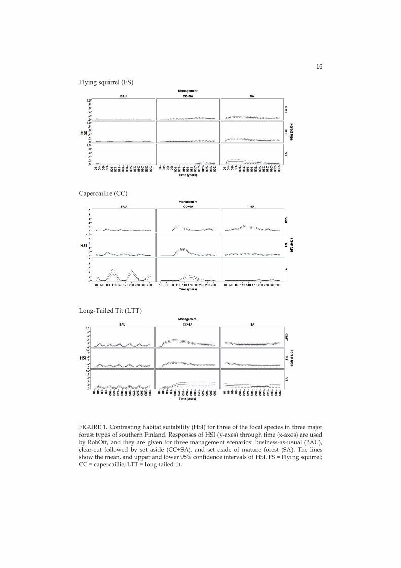
16

Flying squirrel (FS)

Capercaillie (CC)

Long-Tailed Tit (LTT)

FIGURE 1. Contrasting habitat suitability (HSI) for three of the focal species in three major forest types of southern Finland. Responses of HSI (y-axes) through time (x-axes) are used by RobOff, and they are given for three management scenarios: business-as-usual (BAU), clear-cut followed by set aside (CC+SA), and set aside of mature forest (SA). The lines show the mean, and upper and lower 95% confidence intervals of HSI. FS = Flying squirrel; CC = capercaillie; LTT = long-tailed tit.

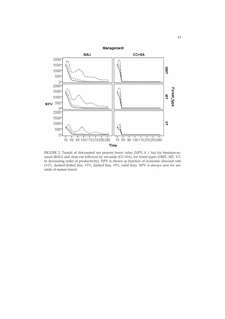
17

FIGURE 2. Trends of discounted net present forest value (NPV, € / ha) for business-as-usual (BAU) and clear-cut followed by set-aside (CC+SA), for forest types (OMT, MT, VT, in decreasing order of productivity). NPV is shown as function of economic discount rate (+1%, dashed-dotted line, +3%, dashed line, +5%, solid line). NPV is always zero for set-aside of mature forest.

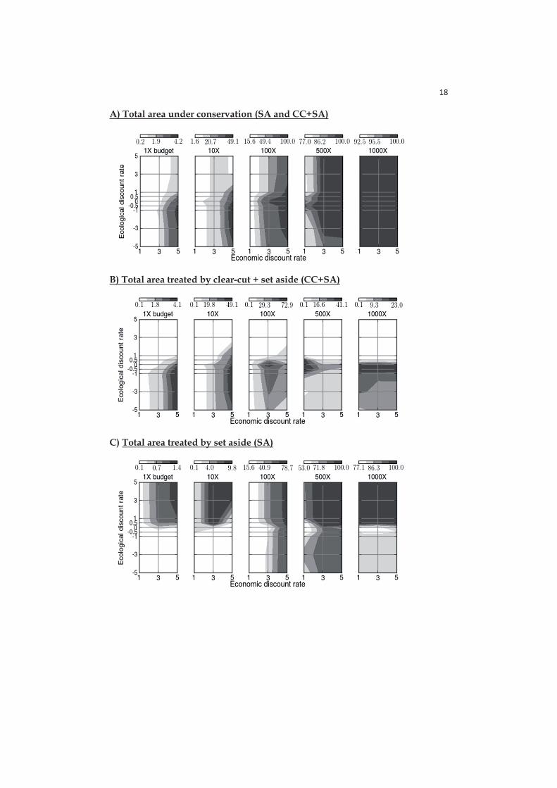
18

A) Total area under conservation (SA and CC+SA)

B) Total area treated by clear-cut + set aside (CC+SA)

C) Total area treated by set aside (SA)

19

FIGURE 3. Effect of time discounting and available budget on optimal allocation of actions, expressed as percentage of area (out of c. 7 M ha total) allocated for conservation. This percentage varies primarily because much more area could be afforded via clear-cut + set aside compared to set aside of mature stands. The upper row gives the total area under conservation; the middle row gives area treated by clear-cut + set aside; the bottom row is for set-aside of mature forest. Area not allocated for conservation (complement of percentage allocated) would be managed following business-as-usual practice. The gray scale indicates allocation at different discount rates; note that its interpretation (scale bars) differs between rows and columns. At the present 1x budget level and within a range of plausible discount rates, the majority of conservation area would go into CC+SA.

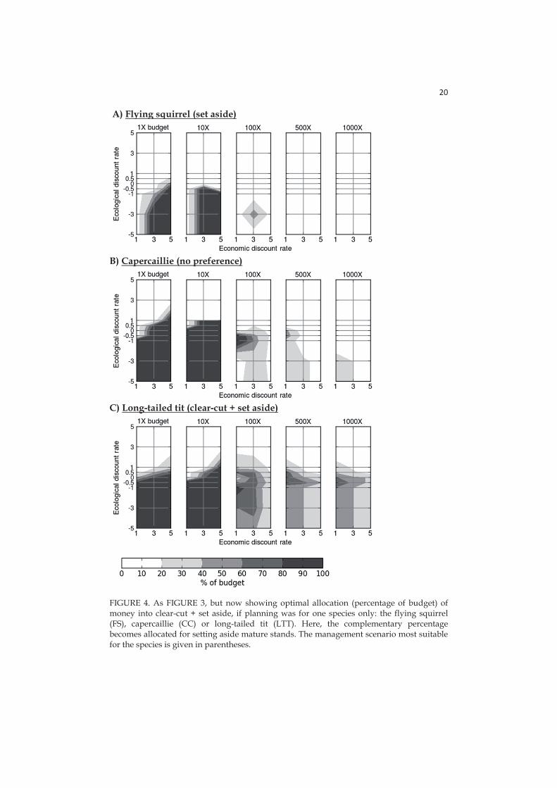
20

A) Flying squirrel (set aside)

B) Capercaillie (no preference)

C) Long-tailed tit (clear-cut + set aside)

FIGURE 4. As FIGURE 3, but now showing optimal allocation (percentage of budget) of money into clear-cut + set aside, if planning was for one species only: the flying squirrel (FS), capercaillie (CC) or long-tailed tit (LTT). Here, the complementary percentage becomes allocated for setting aside mature stands. The management scenario most suitable for the species is given in parentheses.

21

Appendix S1. Forest simulations, limitations and management

Simulation details: In SIMA, the growth of trees is based on diameter growth, which is the product of the potential diameter growth and environmental factors such as temperature sum, within-stand light conditions, soil moisture, and the availability of soil nitrogen. These factors control the demographic processes (birth, growth and death) of tree populations. The death of a tree is determined by crowding, with a consequent reduction in growth, which determines the risk of a tree to die. Stochastic components of SIMA include climate, regeneration and tree death, which in turn feed back to accumulation of dead wood and stand structure, thereby influencing growth of remaining trees. The model structure and parameterization have been described in detail (Kellomäki et al. 1992). Growth model validation has been detailed by Kolström (1998), Kellomäki et al. (2008) and Routa et al. (2011). The simulations were repeated 10 times, a number of replicates proven sufficient by the abovementioned studies to determine the central tendency of demographic processes and variation around it (uncertainty). Simulations limitations: The SIMA simulations do not include natural disturbances such as fire, which should not influence our conclusions: over 300 years the likelihood of natural disturbance is approximately equal for SA and CC+SA, implying increase in stochastic variation in the results without changing the relative utility of management options. Additionally, in Fennoscandia forest fires are strictly controlled, almost eliminating them from the landscape. Management details: The Business-as-usual management (BAU) consists of 60-80 year rotation, site preparation, planting or seeding trees, 1-3 thinnings, final harvest with green tree retention level of 5 trees / ha. Retention trees are subtracted by the total harvestable wood volume. Final harvesting takes place at the stand maturity, i.e. when a certain average tree specific diameter threshold is reached (Yrjölä 2002) References

Kellomäki S., Väisänen H., Hänninen H., Kolström T., Lauhanen R., Mattila U. & Pajari B. 1992. A simulation model for the succession of the boreal forest ecosystem. Silva Fenn. 26: 1–18.

Kellomäki S., Peltola H., Nuutinen T., Korhonen K.T. & Strandman H. 2008. Sensitivity of managed boreal forests in Finland to climate change, with implications for adaptive management. Philos. T. Roy. Soc. B 363: 2339-2349.

Kolström M. 1998. Ecological simulation model for studying diversity of stand structure in boreal forests. Ecol. Model. 111: 17-36.

Routa J., Kellomäki S., Peltola H. & Asikainen A. 2011. Impacts of thinning and fertilization on timber and energy wood production in Norway spruce and Scots pine: scenario analyses based on ecosystem model simulations. Forestry 84: 159-175.

22

Yrjölä T. 2002. Forest management guidelines and practices in Finland, Sweden and Norway European Forest Institute Internal Report 11.

23

Appendix S2. Expanded description of focal species

We selected six focal species to represent the most important dimensions of variation in boreal forest diversity; all these species also are indicator/umbrella species (Mönkkönen et al. 2014).

The capercaillie (Tetrao uralensis) prefers dry pine heaths, and is a game bird with high social and economic value. It is almost extinct from central Europe, near threatened in the latest national red-list of Finland (Rassi et al. 2010) and it is suggested to be a viable surrogate for species richness of breeding forest birds and game animals (Pakkala et al. 2003). Capercaillie leks frequently occur in pine dominated semi-open mature forests with a spruce understory, requiring substantial forest areas of limited human presence (Miettinen et al. 2010).

The flying squirrel (Pteromys volans) is a threatened species associated with mature spruce-dominated mixed forests (VU, Mönkkönen et al. 1997, Rassi et al. 2010). It is an European Union-level priority species for Finland and suggested to be an important umbrella species for forest fauna (Hurme et al. 2008).

The Hazel grouse (Bonasia bonasa) is also a game bird. It inhabits mixed forests and is suggested to be an indicator of adequate levels of deciduous trees at boreal forest landscapes (Angelstam 1992). The Hazel grouse favors dense coniferous or deciduous cover below the canopy (Angelstam et al. 2004).

The long-tailed tit (Aegithalos caudatus) prefers middle-aged to old forests dominated by deciduous trees, where they feed on insects in the canopy (Angelstam et al. 2004).

The three-toed woodpecker (Picoides tridactylus) is a conifer forest species dependent on recently dead or dying wood. It is an important indicator of overall species richness of forest birds (Pakkala et al. 2003, Pakkala 2012).

The lesser-spotted woodpecker (Dendrocopos minor) is a red-listed bird species associated with deciduous, often mid-successional forests. It is dependent on recently dead or dying dead-wood and has been focus of several habitat restoration programs (Angelstam et al. 2004).

These species also encompass variation in successional stages from mid (Hazel grouse, capercaillie, long-tailed tit, lesser-spotted woodpecker) to late (flying squirrel, three-toed woodpecker) successional forests; geographic variation from more southerly (long-tailed tit) to more northerly (three-toed woodpecker) distributed species. In summary, the six focal species were selected to represent a wide spectrum of habitat associations, responses to management, and conservation and social values. References

Angelstam P. 1992. Conservation of communities -- the importance of edges, surroundings and landscape mosaic structure. Pages 4—8 in: L. Hansson, editor. Ecological Principles of Nature Conservation, Applications in Temperate and Boreal Environments. - Elsevier Science Publishers, UK.

Angelstam P., Dönz-Breuss M. & Roberge J.M. 2004. Targets and tools for the maintenance of forest biodiversity – an introduction. Ecol. Bull. 51: 11–24.

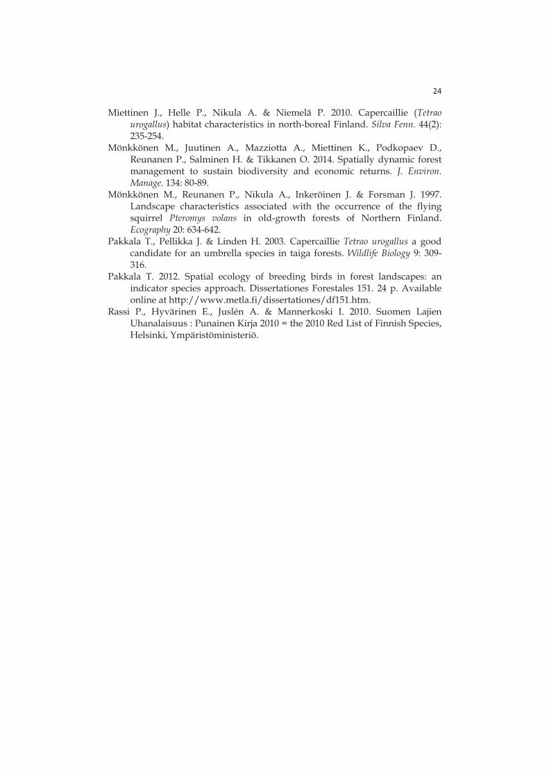
24

Miettinen J., Helle P., Nikula A. & Niemelä P. 2010. Capercaillie (Tetrao urogallus) habitat characteristics in north-boreal Finland. Silva Fenn. 44(2): 235-254.

Mönkkönen M., Juutinen A., Mazziotta A., Miettinen K., Podkopaev D., Reunanen P., Salminen H. & Tikkanen O. 2014. Spatially dynamic forest management to sustain biodiversity and economic returns. J. Environ. Manage. 134: 80-89.

Mönkkönen M., Reunanen P., Nikula A., Inkeröinen J. & Forsman J. 1997. Landscape characteristics associated with the occurrence of the flying squirrel Pteromys volans in old-growth forests of Northern Finland. Ecography 20: 634-642.

Pakkala T., Pellikka J. & Linden H. 2003. Capercaillie Tetrao urogallus a good candidate for an umbrella species in taiga forests. Wildlife Biology 9: 309-316.

Pakkala T. 2012. Spatial ecology of breeding birds in forest landscapes: an indicator species approach. Dissertationes Forestales 151. 24 p. Available online at http://www.metla.fi/dissertationes/df151.htm.

Rassi P., Hyvärinen E., Juslén A. & Mannerkoski I. 2010. Suomen Lajien Uhanalaisuus : Punainen Kirja 2010 = the 2010 Red List of Finnish Species, Helsinki, Ympäristöministeriö.

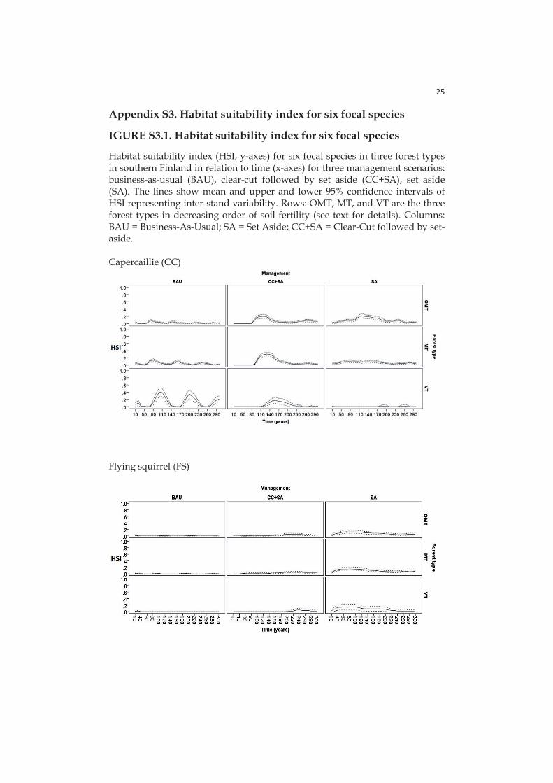
25

Appendix S3. Habitat suitability index for six focal species

IGURE S3.1. Habitat suitability index for six focal species

Habitat suitability index (HSI, y-axes) for six focal species in three forest types in southern Finland in relation to time (x-axes) for three management scenarios: business-as-usual (BAU), clear-cut followed by set aside (CC+SA), set aside (SA). The lines show mean and upper and lower 95% confidence intervals of HSI representing inter-stand variability. Rows: OMT, MT, and VT are the three forest types in decreasing order of soil fertility (see text for details). Columns: BAU = Business-As-Usual; SA = Set Aside; CC+SA = Clear-Cut followed by set-aside. Capercaillie (CC)

Flying squirrel (FS)

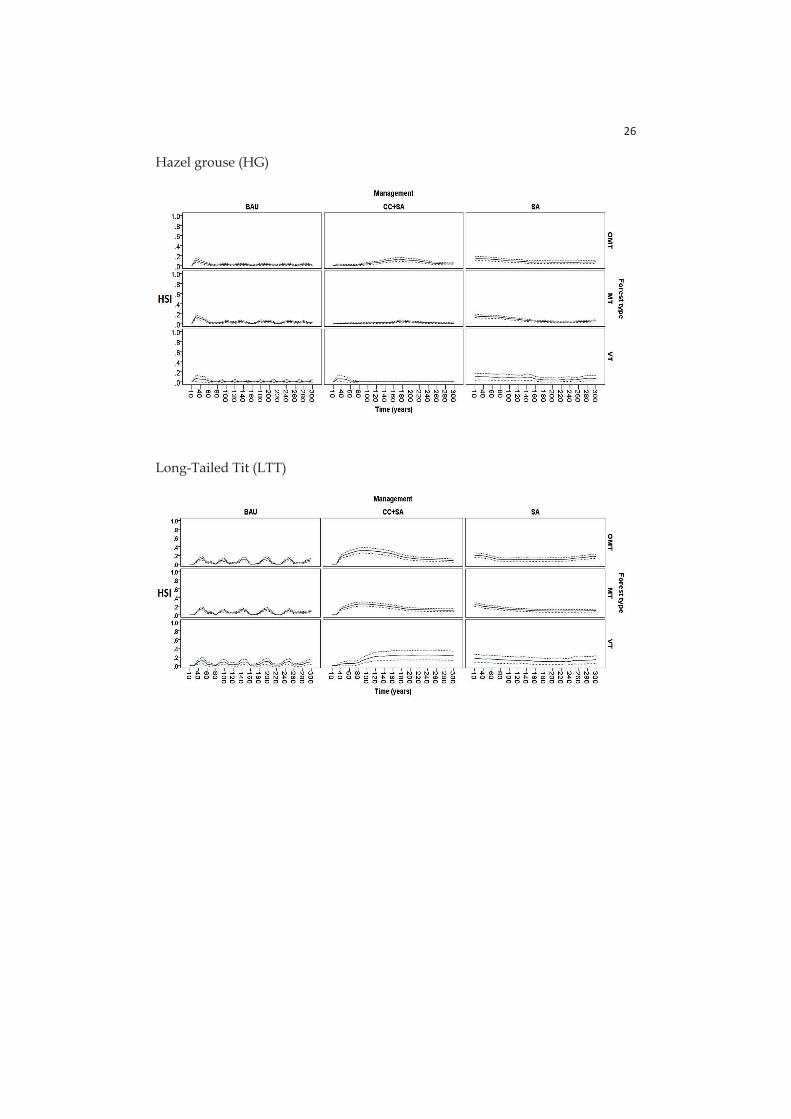
26

Hazel grouse (HG)

Long-Tailed Tit (LTT)

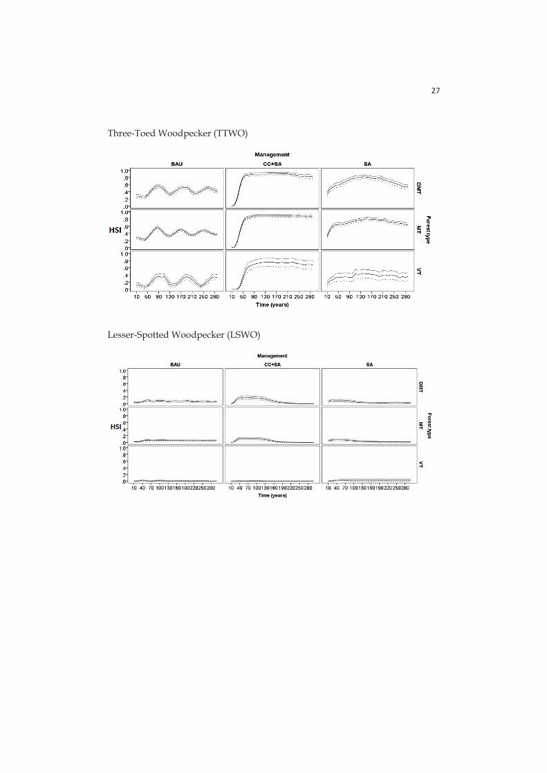
27

Three-Toed Woodpecker (TTWO)

Lesser-Spotted Woodpecker (LSWO)