Government Spending & Fiscal

Policy

Presented by:

Zahra Abdulkadir Amin

CONTENTS

Government Spending

Government Deficit

Adjusting the deficit for inflation & the cycle

Government Deficit and the national debt

The stance of fiscal policy

Applications on Kuwait

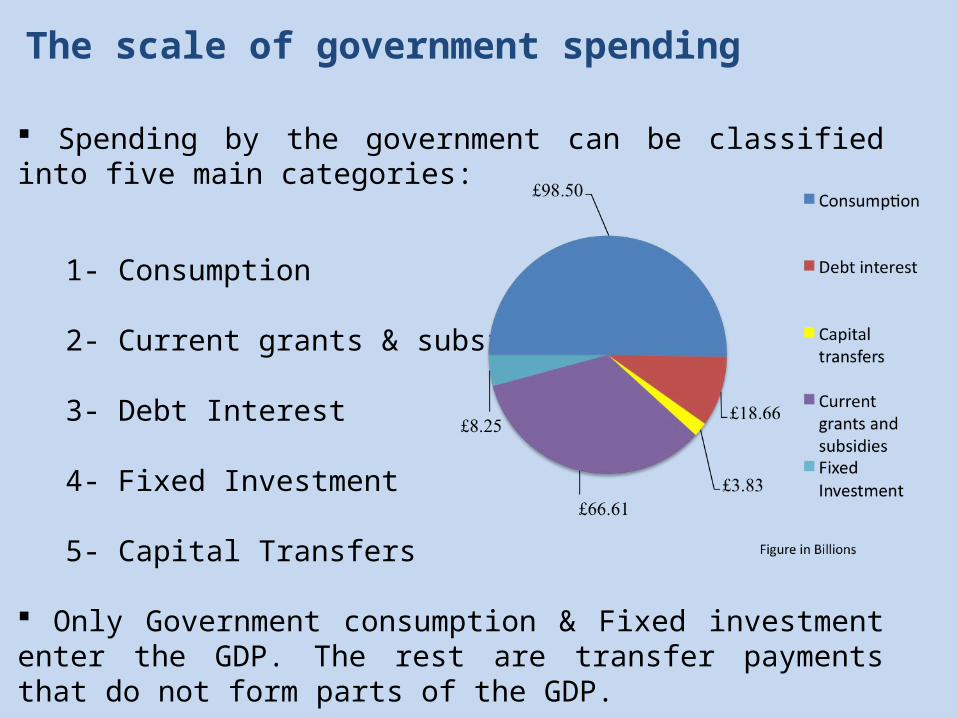
The scale of government spending

Spending by the government can be classified into five main categories:

1- Consumption

2- Current grants & subsidies

3- Debt Interest

4- Fixed Investment

5- Capital Transfers

Only Government consumption & Fixed investment enter the GDP. The rest are transfer payments that do not form parts of the GDP.

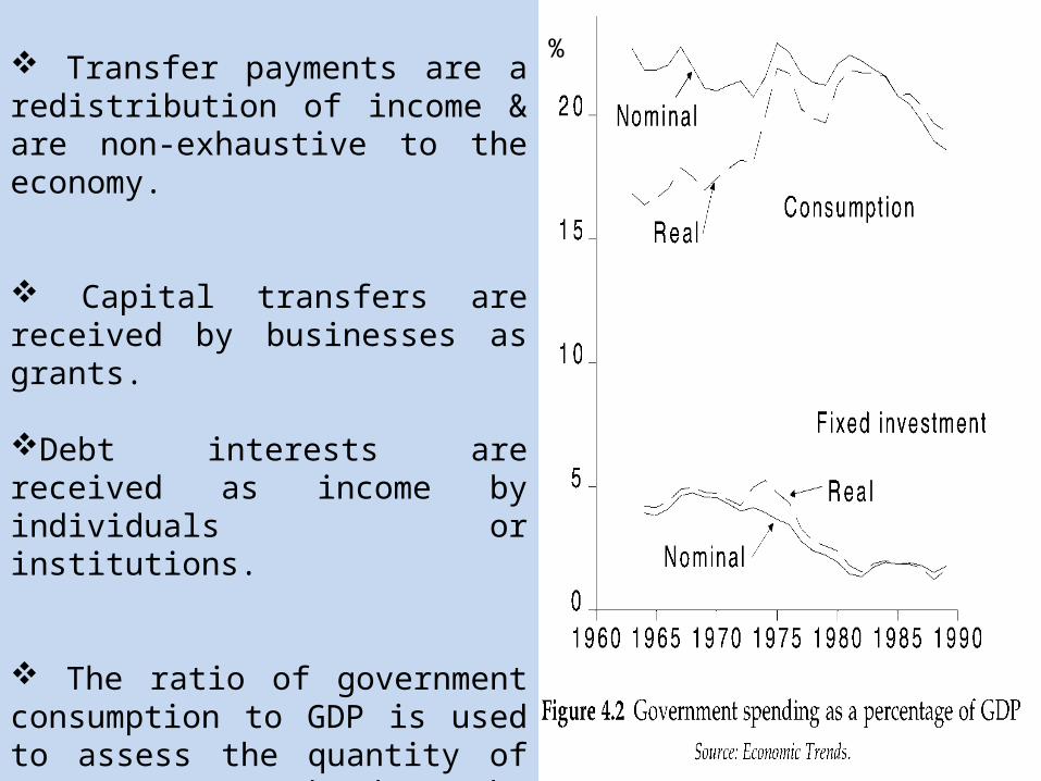
Transfer payments are a redistribution of income & are non-exhaustive to the economy.

Capital transfers are received by businesses as grants.

Debt interests are received as income by individuals or institutions.

The ratio of government consumption to GDP is used to assess the quantity of resources used by the government.

%

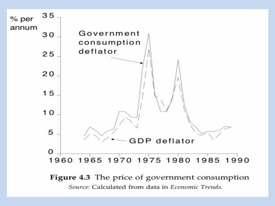
When measured using constant and current prices, the ratio of government expenditures to GDP exhibit different fluctuation rates.

The price of government consumption has risen faster than the GDP deflator.

The reason for that is that it’s difficult to measure improvements in the quality of government services.

Improvements are thus measured by the government spending, by adding up the resources used, which fails to reflect the productivity growth.

Government investments in the UK roughly halved remaining very law since the 1970s.

The fall in government investment happened because the government was obliged to reduce its spending.

Government spending changes not only as a response to changes in economic policy, but also as a response to structural changes in the economy.

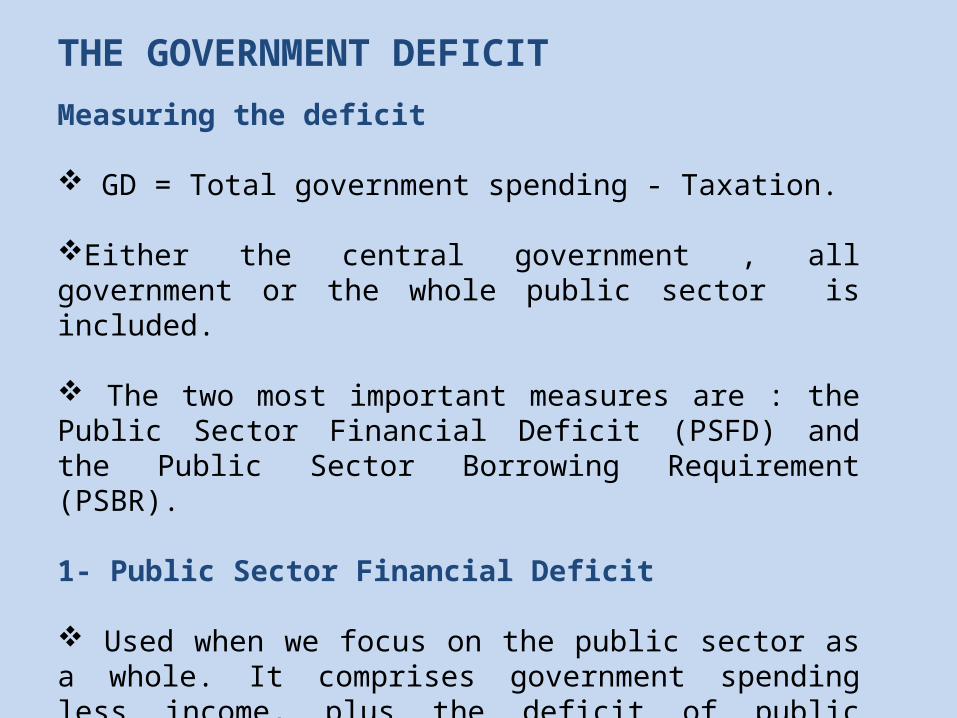
THE GOVERNMENT DEFICIT

Measuring the deficit

GD = Total government spending - Taxation.

Either the central government , all government or the whole public sector is included.

The two most important measures are : the Public Sector Financial Deficit (PSFD) and the Public Sector Borrowing Requirement (PSBR).

1- Public Sector Financial Deficit

Used when we focus on the public sector as a whole. It comprises government spending less income, plus the deficit of public corporations.

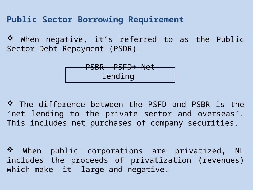
Public Sector Borrowing Requirement

When negative, it’s referred to as the Public Sector Debt Repayment (PSDR).

The difference between the PSFD and PSBR is the ‘net lending to the private sector and overseas’. This includes net purchases of company securities.

When public corporations are privatized, NL includes the proceeds of privatization (revenues) which make it large and negative.

PSBR= PSFD+ Net Lending

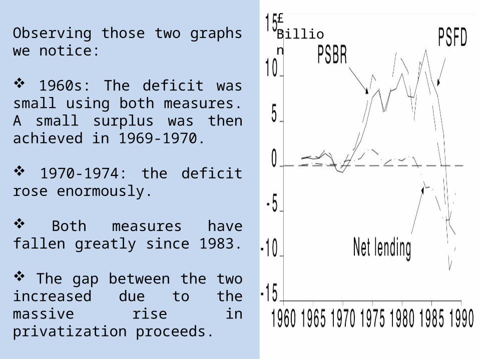
Observing those two graphs we notice:

1960s: The deficit was small using both measures. A small surplus was then achieved in 1969-1970.

1970-1974: the deficit rose enormously.

Both measures have fallen greatly since 1983.

The gap between the two increased due to the massive rise in privatization proceeds.

£ Billion

Why does the government deficit matter?

If it’s not financed by an increase in

money supply, it must be financed by

borrowing.

Large scale borrowing raises interest

rates causing the crowding out effect.

How to finance the deficit depends on

the public view of shares and bonds.

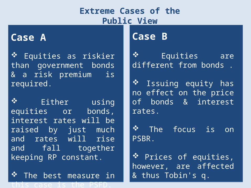
Extreme Cases of the Public View

Case A

Equities as riskier than government bonds & a risk premium is required.

Either using equities or bonds, interest rates will be raised by just much and rates will rise and fall together keeping RP constant.

The best measure in this case is the PSFD.

Case B

Equities are different from bonds .

Issuing equity has no effect on the price of bonds & interest rates.

The focus is on PSBR.

Prices of equities, however, are affected & thus Tobin's q.

Adjusting for inflation and the cycle

Government deficit needs to be adjusted for the following:

1- Inflation tax

Inflation tax is the economic disadvantage suffered by holders of cash and its equivalents due to the effects of inflation.

Since government are the biggest debtors, inflation tax transfers resources from the private sector to the government.

Only the real cost of interest payments should.

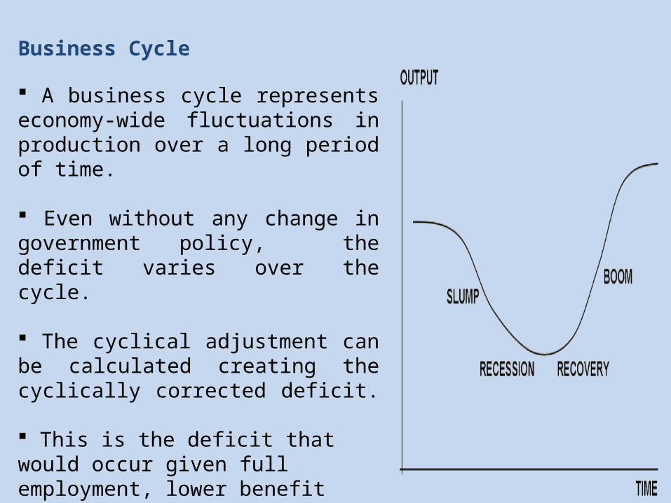
Business Cycle

A business cycle represents economy-wide fluctuations in production over a long period of time.

Even without any change in government policy, the deficit varies over the cycle.

The cyclical adjustment can be calculated creating the cyclically corrected deficit.

This is the deficit that would occur given full employment, lower benefit payments and higher tax revenues.

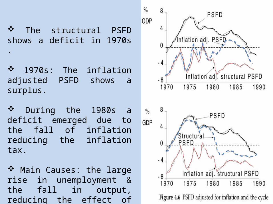
The structural PSFD shows a deficit in 1970s .

1970s: The inflation adjusted PSFD shows a surplus.

During the 1980s a deficit emerged due to the fall of inflation reducing the inflation tax.

Main Causes: the large rise in unemployment & the fall in output, reducing the effect of the contractionary policy.

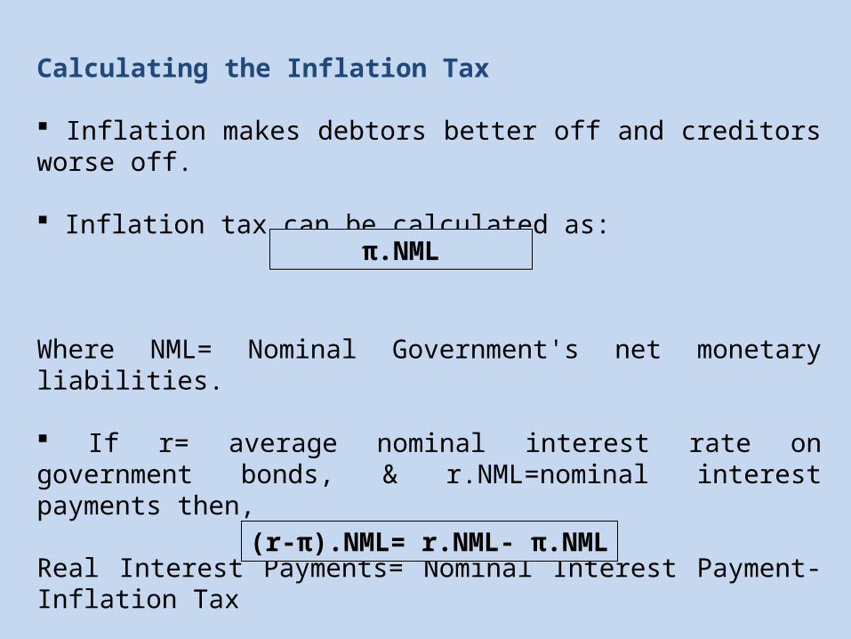
Calculating the Inflation Tax

Inflation makes debtors better off and creditors worse off.

Inflation tax can be calculated as:

Where NML= Nominal Government's net monetary liabilities.

If r= average nominal interest rate on government bonds, & r.NML=nominal interest payments then,

Real Interest Payments= Nominal Interest Payment- Inflation Tax

π.NML

(r-π).NML= r.NML- π.NML

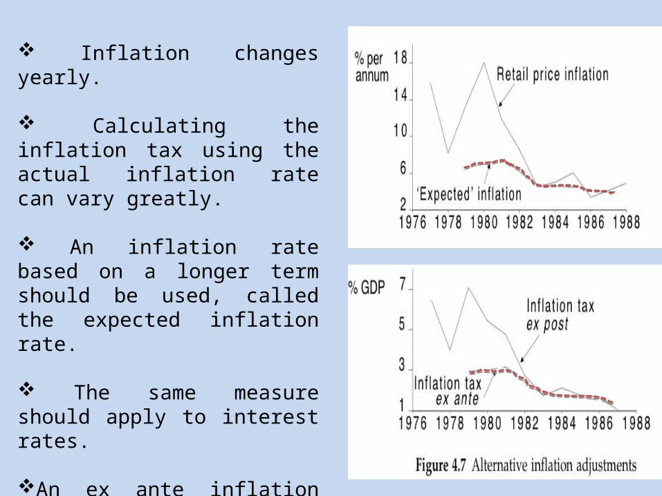
Inflation changes yearly. Calculating the inflation tax using the actual inflation rate can vary greatly.

An inflation rate based on a longer term should be used, called the expected inflation rate.

The same measure should apply to interest rates.

An ex ante inflation tax can be calculated using expected interest rates.

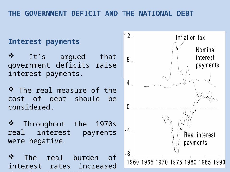
Interest payments

It’s argued that government deficits raise interest payments.

The real measure of the cost of debt should be considered.

Throughout the 1970s real interest payments were negative.

The real burden of interest rates increased sharply since 1980s.

THE GOVERNMENT DEFICIT AND THE NATIONAL DEBT

Government Debt

Note that:

It’s possible to run a deficit without the real value of the debt increasing if inflation is reducing its real vale.

Real Debt will increase only if the inflation-adjusted balance is negative.

If GDP grows at a rate of 12%, the government can run a deficit of 12% of the national debt each year.

If the growth rate of GDP (g) exceeds the real interest rate in the long run, the ratio of government debt to GDP will converge to a stable equilibrium.

1960s: National debt fell as a proportion of GDP and since then has been approximately constant.

The ratio of debt to GDP is self limiting.

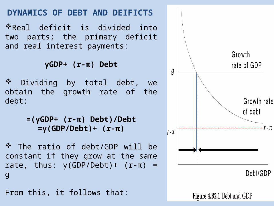
Real deficit is divided into two parts; the primary deficit and real interest payments:

γGDP+ (r-π) Debt

Dividing by total debt, we obtain the growth rate of the debt:

=(γGDP+ (r-π) Debt)/Debt=γ(GDP/Debt)+ (r-π)

The ratio of debt/GDP will be constant if they grow at the same rate, thus: γ(GDP/Debt)+ (r-π) = g

From this, it follows that:

Debt/GDP= γ/(g-r-π)

DYNAMICS OF DEBT AND DEIFICTS

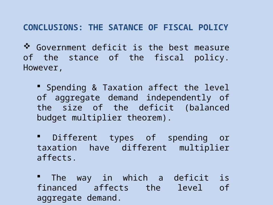
CONCLUSIONS: THE SATANCE OF FISCAL POLICY

Government deficit is the best measure of the stance of the fiscal policy. However,

Spending & Taxation affect the level of aggregate demand independently of the size of the deficit (balanced budget multiplier theorem).

Different types of spending or taxation have different multiplier affects.

The way in which a deficit is financed affects the level of aggregate demand.

Applications on Kuwait

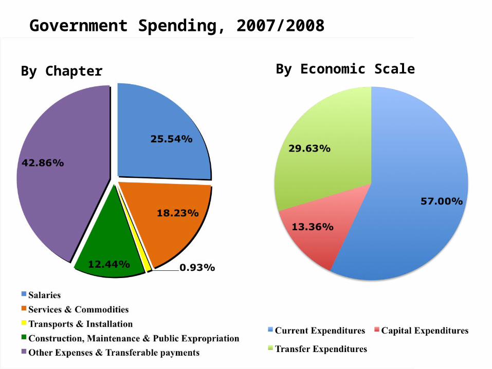
Government Spending, 2007/2008

By Chapter By Economic Scale

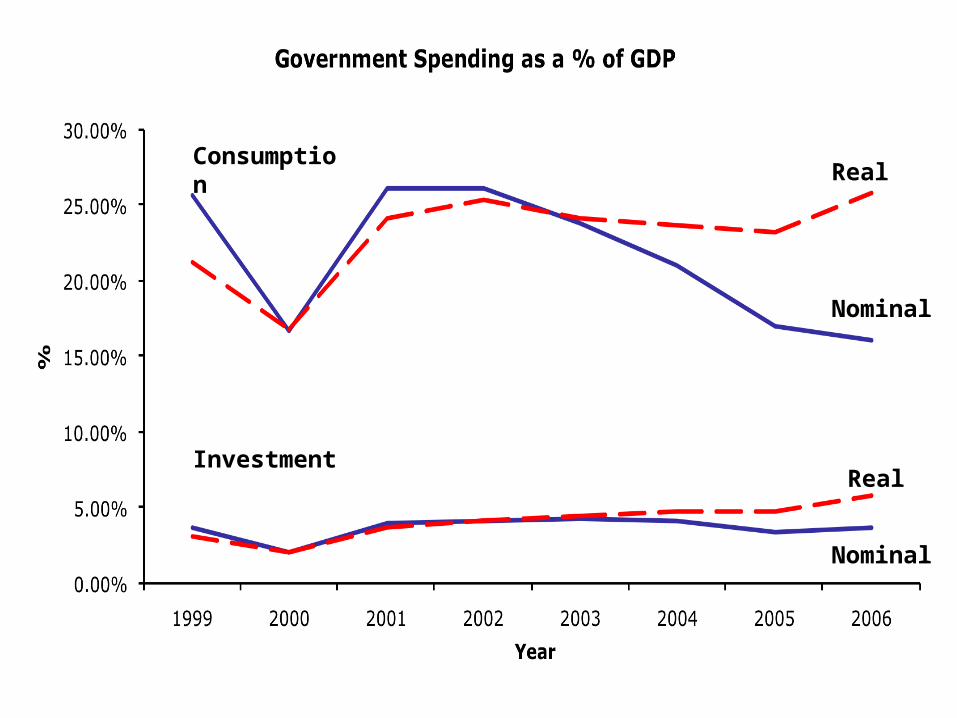
Consumption

Investment

Real

Real

Nominal

Nominal

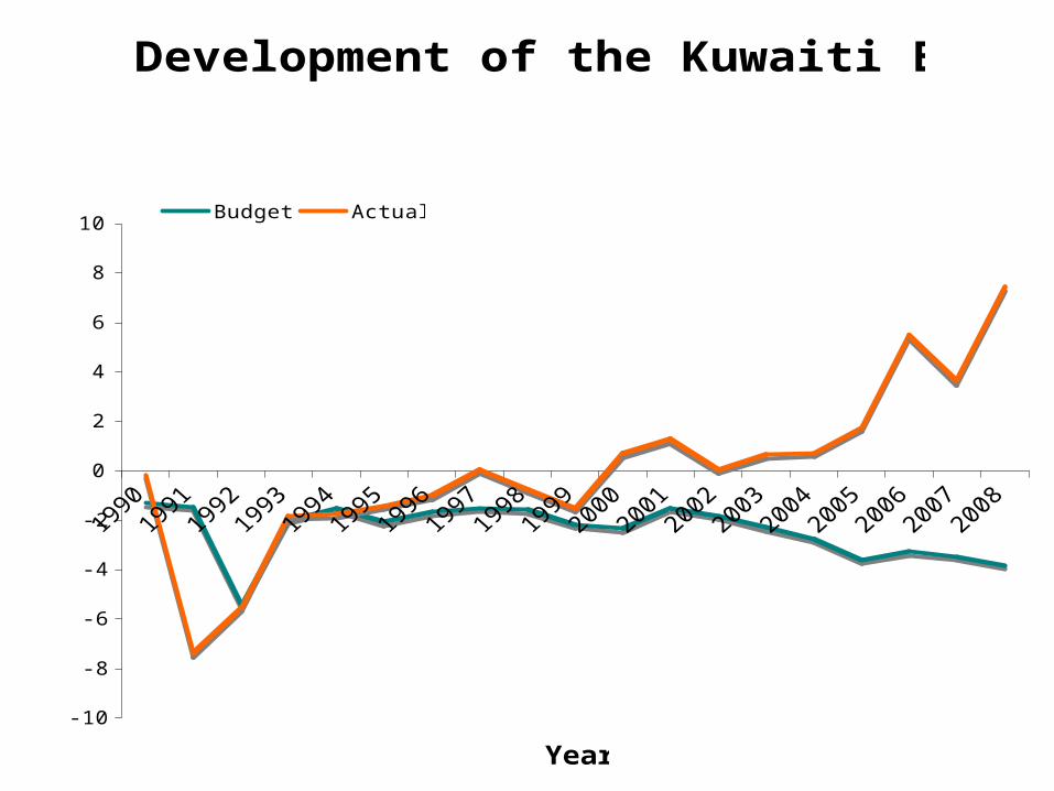
Development of the Kuwaiti Budget

-10

-8

-6

-4

-2

0

2

4

6

8

10

Year

Billio

n K

D

Budget Actual

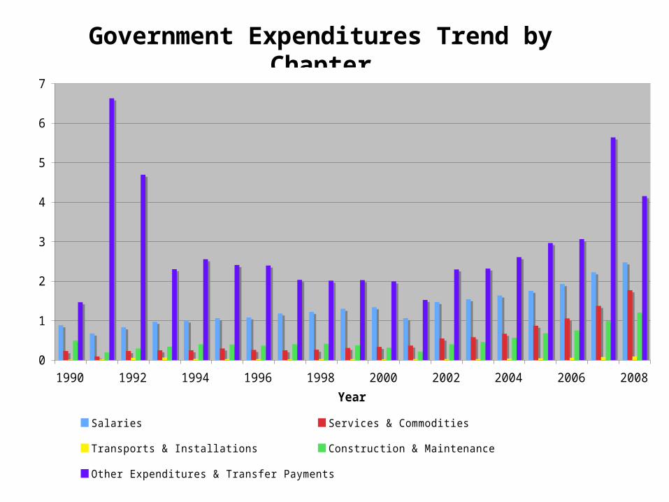
Government Expenditures Trend by Chapter

0

1

2

3

4

5

6

7

1990 1992 1994 1996 1998 2000 2002 2004 2006 2008

Year

Bil

lio

n K

D

Salaries Services & Commodities

Transports & Installations Construction & Maintenance

Other Expenditures & Transfer Payments

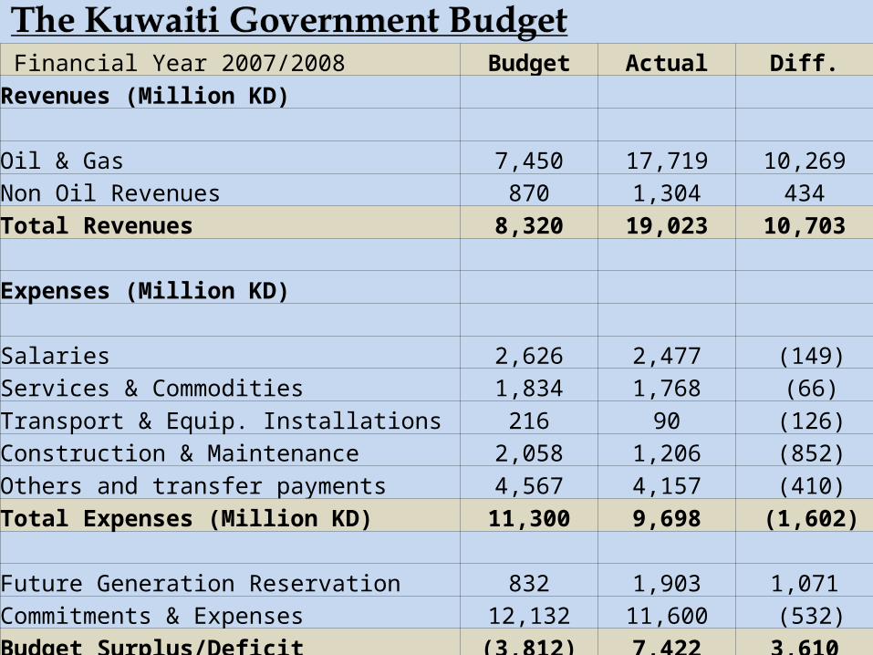
 Financial Year 2007/2008 Budget Actual Diff.Revenues (Million KD)             Oil & Gas 7,450 17,719 10,269 Non Oil Revenues 870 1,304 434 Total Revenues 8,320 19,023 10,703        Expenses (Million KD)             Salaries 2,626 2,477 (149)Services & Commodities 1,834 1,768 (66)Transport & Equip. Installations 216 90 (126)Construction & Maintenance 2,058 1,206 (852)Others and transfer payments 4,567 4,157 (410)Total Expenses (Million KD) 11,300 9,698 (1,602)       Future Generation Reservation 832 1,903 1,071 Commitments & Expenses 12,132 11,600 (532)Budget Surplus/Deficit (3,812) 7,422 3,610

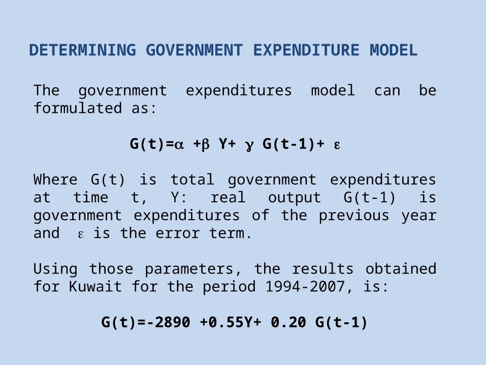
DETERMINING GOVERNMENT EXPENDITURE MODEL

The government expenditures model can be formulated as:

G(t)= + Y+ G(t-1)+

Where G(t) is total government expenditures at time t, Y: real output G(t-1) is government expenditures of the previous year and is the error term.

Using those parameters, the results obtained for Kuwait for the period 1994-2007, is:

G(t)=-2890 +0.55Y+ 0.20 G(t-1)

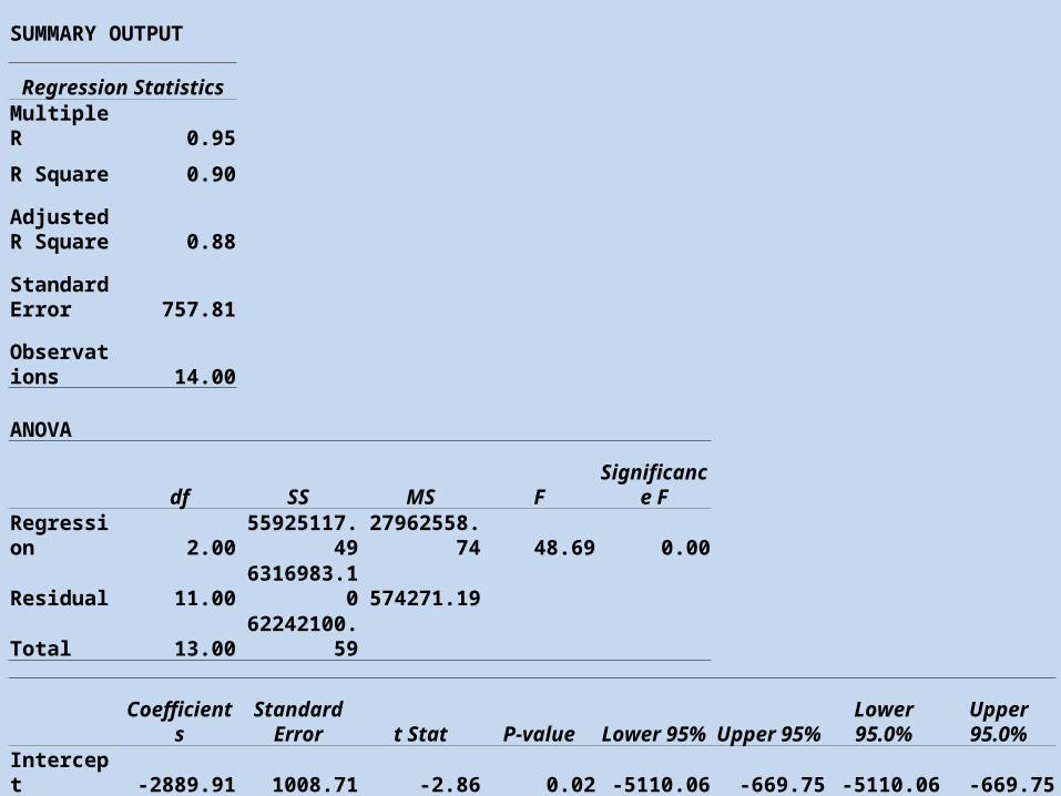
SUMMARY OUTPUT

Regression Statistics

Multiple R 0.95

R Square 0.90

Adjusted R Square 0.88

Standard Error 757.81

Observations 14.00

ANOVA

  df SS MS FSignificance

F

Regression 2.00 55925117.49 27962558.74 48.69 0.00

Residual 11.00 6316983.10 574271.19

Total 13.00 62242100.59      

  CoefficientsStandard

Error t Stat P-value Lower 95% Upper 95%Lower 95.0% Upper 95.0%

Intercept -2889.91 1008.71 -2.86 0.02 -5110.06 -669.75 -5110.06 -669.75X Variable 1 0.55 0.15 3.77 0.00 0.23 0.88 0.23 0.88X Variable 2 0.20 0.25 0.81 0.43 -0.35 0.76 -0.35 0.76

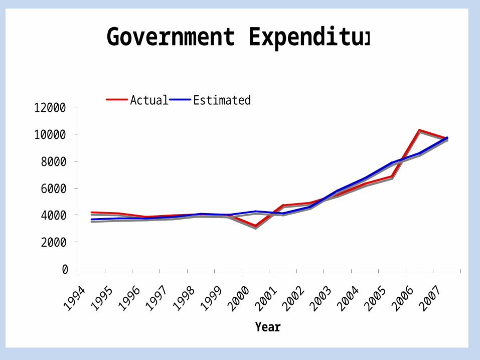
Government Expenditures

0

2000

4000

6000

8000

10000

12000

Year

Mill

ion

KD

Actual Estimated

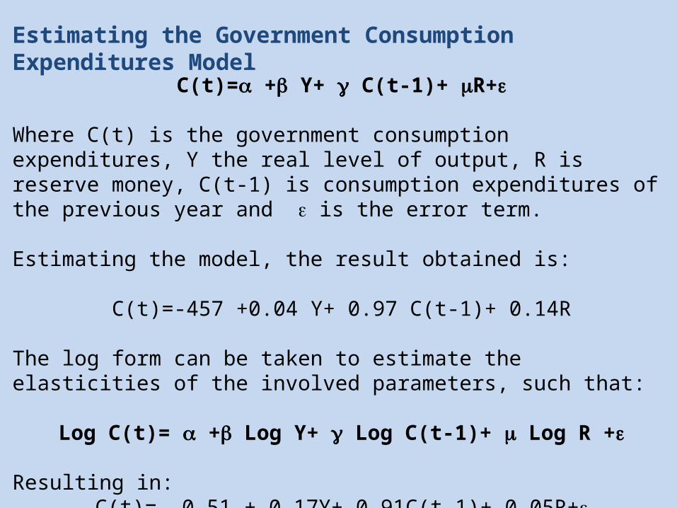
Estimating the Government Consumption Expenditures Model

C(t)= + Y+ C(t-1)+ R+

Where C(t) is the government consumption expenditures, Y the real level of output, R is reserve money, C(t-1) is consumption expenditures of the previous year and is the error term.

Estimating the model, the result obtained is:

C(t)=-457 +0.04 Y+ 0.97 C(t-1)+ 0.14R

The log form can be taken to estimate the elasticities of the involved parameters, such that:

Log C(t)= + Log Y+ Log C(t-1)+ Log R +

Resulting in:C(t)= -0.51 + 0.17Y+ 0.91C(t-1)+ 0.05R+

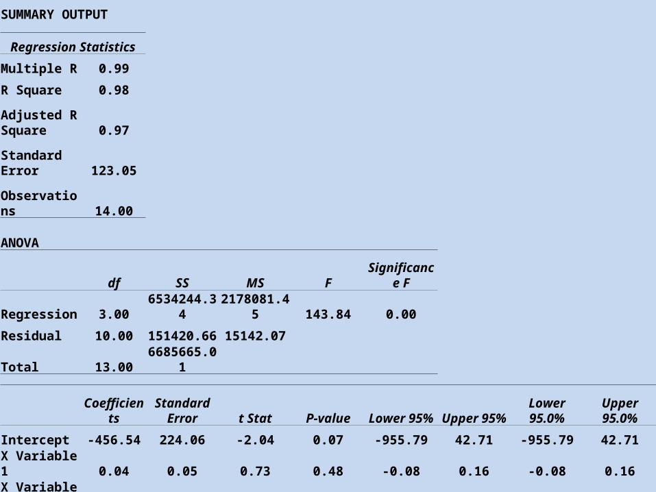
SUMMARY OUTPUT

Regression Statistics

Multiple R 0.99

R Square 0.98

Adjusted R Square 0.97

Standard Error 123.05

Observations 14.00

ANOVA

  df SS MS FSignificance

F

Regression 3.00 6534244.34 2178081.45 143.84 0.00

Residual 10.00 151420.66 15142.07

Total 13.00 6685665.01      

 Coefficient

sStandard

Error t Stat P-value Lower 95% Upper 95% Lower 95.0% Upper 95.0%

Intercept -456.54 224.06 -2.04 0.07 -955.79 42.71 -955.79 42.71

X Variable 1 0.04 0.05 0.73 0.48 -0.08 0.16 -0.08 0.16

X Variable 2 0.97 0.29 3.37 0.01 0.33 1.62 0.33 1.62

X Variable 3 0.14 0.08 1.77 0.11 -0.04 0.32 -0.04 0.32

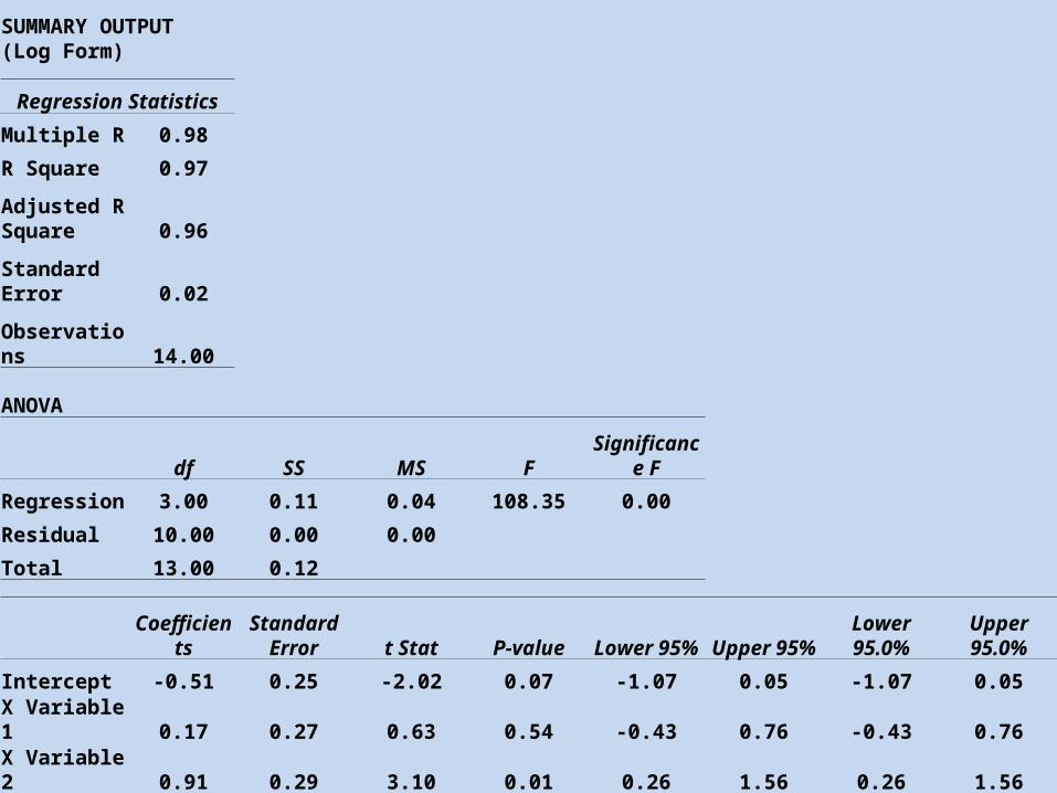
SUMMARY OUTPUT (Log Form)

Regression StatisticsMultiple R 0.98R Square 0.97Adjusted R Square 0.96Standard Error 0.02

Observations 14.00

ANOVA

  df SS MS FSignificance

FRegression 3.00 0.11 0.04 108.35 0.00Residual 10.00 0.00 0.00Total 13.00 0.12      

 Coefficient

sStandard

Error t Stat P-value Lower 95% Upper 95% Lower 95.0% Upper 95.0%Intercept -0.51 0.25 -2.02 0.07 -1.07 0.05 -1.07 0.05X Variable 1 0.17 0.27 0.63 0.54 -0.43 0.76 -0.43 0.76X Variable 2 0.91 0.29 3.10 0.01 0.26 1.56 0.26 1.56X Variable 3 0.05 0.03 1.59 0.14 -0.02 0.13 -0.02 0.13

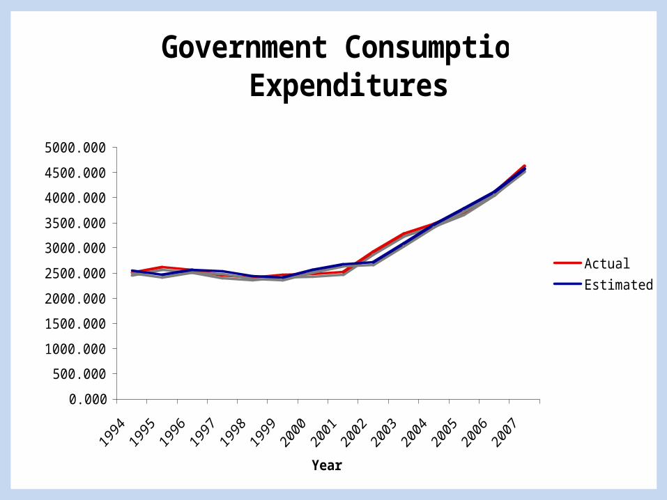
Government Consumption Expenditures

0.000

500.000

1000.000

1500.000

2000.000

2500.000

3000.000

3500.000

4000.000

4500.000

5000.000

Year

Mil

lio

n K

D

Actual

Estimated