Govinda Timilsina

The World Bank, Washington, DC

Skopje, Macedonia

March 01, 2011

Global and Country Specific CGE Models at the World Bank for Climate Change Analysis

Presentation Outline

Introduction Global CGE Model Data for Global CGE Model Single Country CGE Model Data for Single Country CGE Model

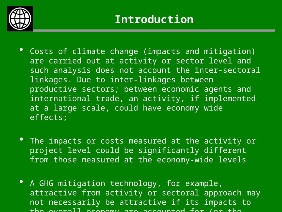
Introduction

• Costs of climate change (impacts and mitigation) are carried out at activity or sector level and such analysis does not account the inter-sectoral linkages. Due to inter-linkages between productive sectors; between economic agents and international trade, an activity, if implemented at a large scale, could have economy wide effects;

• The impacts or costs measured at the activity or project level could be significantly different from those measured at the economy-wide levels

• A GHG mitigation technology, for example, attractive from activity or sectoral approach may not necessarily be attractive if its impacts to the overall economy are accounted for (or the rankings of GHG mitigation options could change)

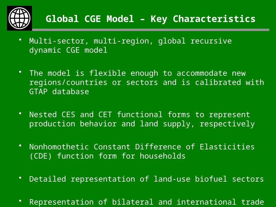
Global CGE Model – Key Characteristics

• Multi-sector, multi-region, global recursive dynamic CGE model

• The model is flexible enough to accommodate new regions/countries or sectors and is calibrated with GTAP database

• Nested CES and CET functional forms to represent production behavior and land supply, respectively

• Nonhomothetic Constant Difference of Elasticities (CDE) function form for households

• Detailed representation of land-use biofuel sectors

• Representation of bilateral and international trade

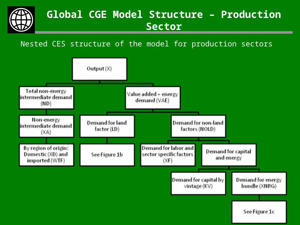
Global CGE Model Structure – Production Sector

Nested CES structure of the model for production sectors

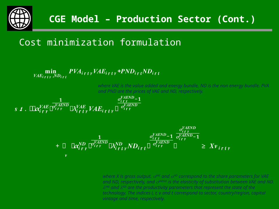
CGE Model – Production Sector (Cont.)

𝐦𝐢𝐧𝑽𝑨𝑬𝒊,𝒓,𝒕,𝒗, 𝑵𝑫𝒊,𝒓,𝒕 𝑷𝑽𝑨𝒊,𝒓,𝒕,𝒗𝑽𝑨𝑬𝒊,𝒓,𝒕,𝒗+𝑷𝑵𝑫𝒊,𝒓,𝒕𝑵𝑫𝒊,𝒓,𝒕

𝒔.𝒕. ൫𝜶𝒊,𝒓,𝒗𝑽𝑨𝑬൯ 𝟏𝝈𝒊,𝒓,𝒗𝑽𝑨𝑬𝑵𝑫൫𝝀𝒊,𝒓,𝒕,𝒗𝑽𝑨𝑬 𝑽𝑨𝑬𝒊,𝒓,𝒕,𝒗൯

𝝈𝒊,𝒓,𝒗𝑽𝑨𝑬𝑵𝑫−𝟏𝝈𝒊,𝒓,𝒗𝑽𝑨𝑬𝑵𝑫

+ ൫𝜶𝒊,𝒓,𝒗𝑵𝑫൯𝟏𝝈𝒊,𝒓,𝒗𝑽𝑨𝑬𝑵𝑫

൫𝝀𝒊,𝒓,𝒕,𝒗𝑵𝑫 𝑵𝑫𝒊,𝒓,𝒕൯𝝈𝒊,𝒓,𝒗𝑽𝑨𝑬𝑵𝑫−𝟏𝝈𝒊,𝒓,𝒗𝑽𝑨𝑬𝑵𝑫

𝒗 𝝈𝒊,𝒓,𝒗𝑽𝑨𝑬𝑵𝑫𝝈𝒊,𝒓,𝒗𝑽𝑨𝑬𝑵𝑫−𝟏 ≥ 𝑿𝒗𝒊,𝒓,𝒕,𝒗

where X is gross output. VAE and ND correspond to the share parameters for VAE and ND, respectively, and VAEND is the elasticity of substitution between VAE and ND. VAE and ND are the productivity parameters that represent the state of the technology. The indices i, r, v and t correspond to sector, country/region, capital vintage and time, respectively.

where VAE is the value added and energy bundle, ND is the non energy bundle. PVA and PND are the prices of VAE and ND, respectively.

Cost minimization formulation

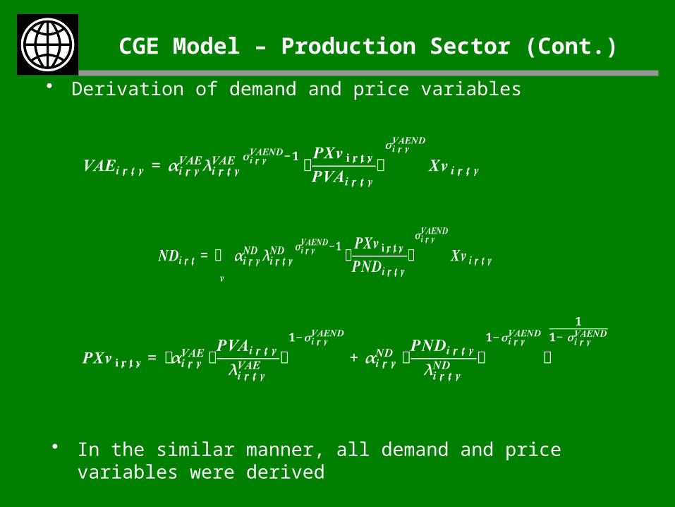
CGE Model – Production Sector (Cont.)

• Derivation of demand and price variables

𝑽𝑨𝑬𝒊,𝒓,𝒕,𝒗 = 𝜶𝒊,𝒓,𝒗𝑽𝑨𝑬𝝀𝒊,𝒓,𝒕,𝒗𝑽𝑨𝑬 𝝈𝒊,𝒓,𝒗𝑽𝑨𝑬𝑵𝑫−𝟏ቆ

𝑷𝑿𝒗𝐢,𝐫,𝐭,𝐯𝑷𝑽𝑨𝒊,𝒓,𝒕,𝒗ቇ𝝈𝒊,𝒓,𝒗𝑽𝑨𝑬𝑵𝑫𝑿𝒗𝒊,𝒓,𝒕,𝒗

𝑵𝑫𝒊,𝒓,𝒕 = 𝜶𝒊,𝒓,𝒗𝑵𝑫 𝝀𝒊,𝒓,𝒕,𝒗𝑵𝑫 𝝈𝒊,𝒓,𝒗𝑽𝑨𝑬𝑵𝑫−𝟏ቆ

𝑷𝑿𝒗𝐢,𝐫,𝐭,𝐯𝑷𝑵𝑫𝒊,𝒓,𝒕,𝒗ቇ𝝈𝒊,𝒓,𝒗𝑽𝑨𝑬𝑵𝑫𝑿𝒗𝒊,𝒓,𝒕,𝒗𝒗

𝑷𝑿𝒗𝐢,𝐫,𝐭,𝐯= 𝜶𝒊,𝒓,𝒗𝑽𝑨𝑬ቆ𝑷𝑽𝑨𝒊,𝒓,𝒕,𝒗𝝀𝒊,𝒓,𝒕,𝒗𝑽𝑨𝑬 ቇ

𝟏−𝝈𝒊,𝒓,𝒗𝑽𝑨𝑬𝑵𝑫 + 𝜶𝒊,𝒓,𝒗𝑵𝑫 ቆ𝑷𝑵𝑫𝒊,𝒓,𝒕,𝒗𝝀𝒊,𝒓,𝒕,𝒗𝑵𝑫 ቇ

𝟏−𝝈𝒊,𝒓,𝒗𝑽𝑨𝑬𝑵𝑫𝟏𝟏− 𝝈𝒊,𝒓,𝒗𝑽𝑨𝑬𝑵𝑫

• In the similar manner, all demand and price variables were derived

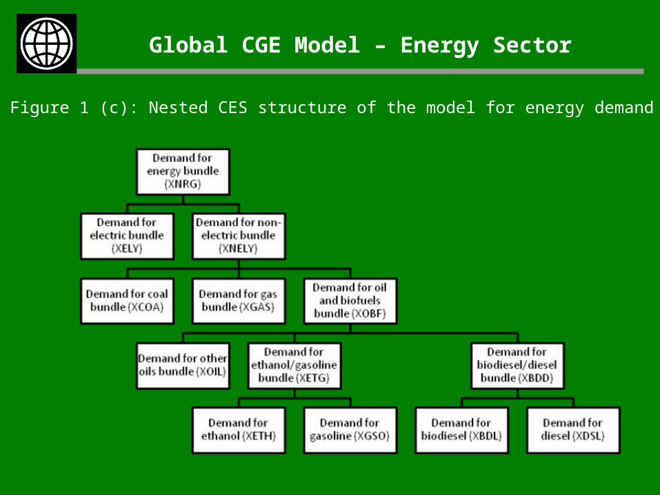
Global CGE Model – Energy Sector

Figure 1 (c): Nested CES structure of the model for energy demand

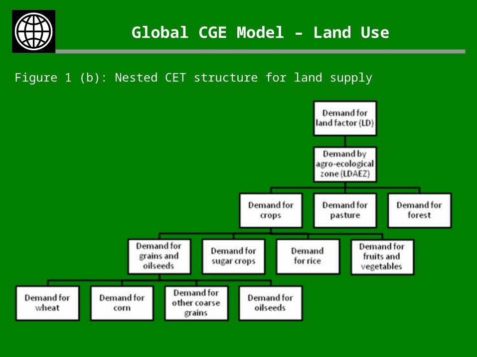
Global CGE Model – Land Use

Figure 1 (b): Nested CET structure for land supply

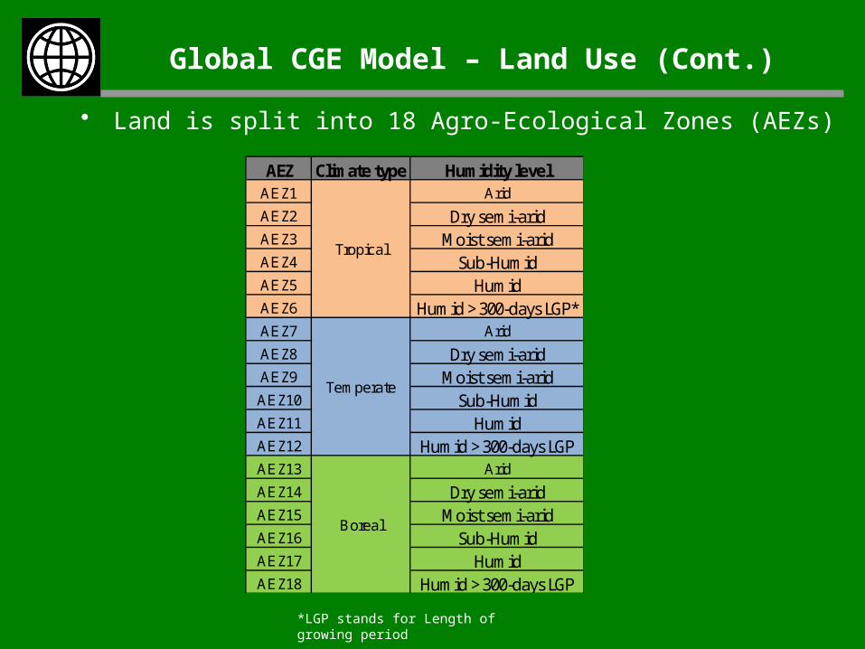
Global CGE Model – Land Use (Cont.)

AEZ Climate type Humidity levelAEZ1 Arid

AEZ2 Dry semi-aridAEZ3 Moist semi-aridAEZ4 Sub-HumidAEZ5 HumidAEZ6 Humid > 300-days LGP*AEZ7 Arid

AEZ8 Dry semi-aridAEZ9 Moist semi-aridAEZ10 Sub-HumidAEZ11 HumidAEZ12 Humid > 300-days LGPAEZ13 Arid

AEZ14 Dry semi-aridAEZ15 Moist semi-aridAEZ16 Sub-HumidAEZ17 HumidAEZ18 Humid > 300-days LGP

Tropical

Temperate

Boreal

*LGP stands for Length of growing period

• Land is split into 18 Agro-Ecological Zones (AEZs)

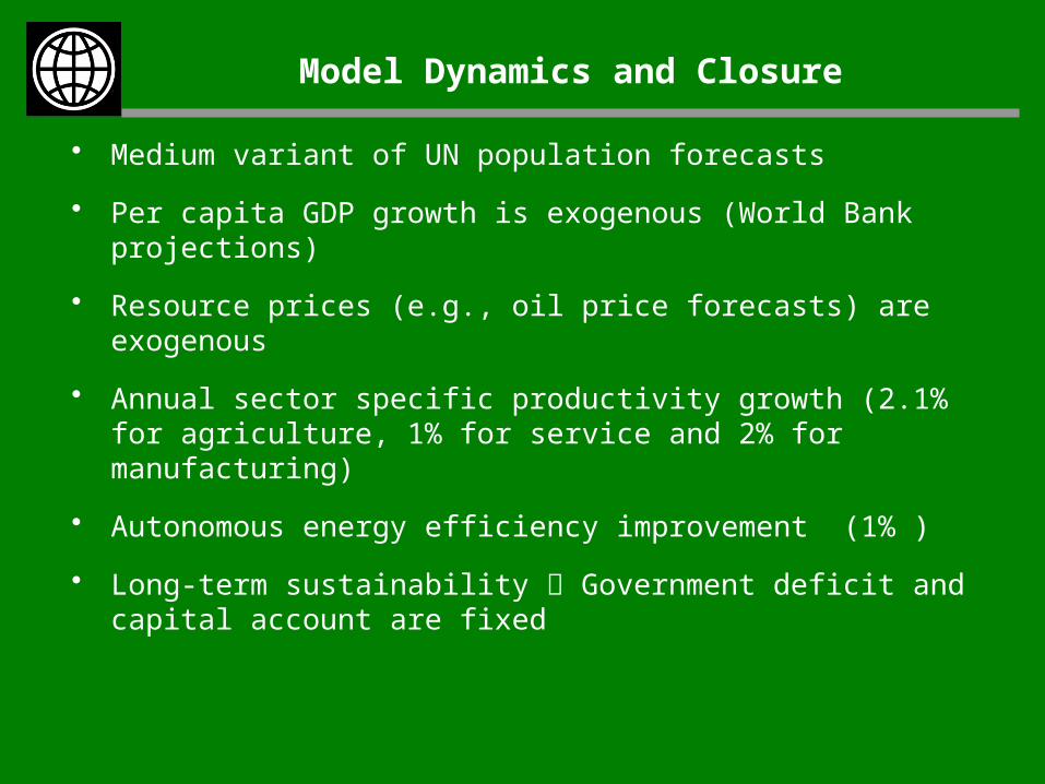
Model Dynamics and Closure

• Medium variant of UN population forecasts

• Per capita GDP growth is exogenous (World Bank projections)

• Resource prices (e.g., oil price forecasts) are exogenous

• Annual sector specific productivity growth (2.1% for agriculture, 1% for service and 2% for manufacturing)

• Autonomous energy efficiency improvement (1% )

• Long-term sustainability Government deficit and capital account are fixed

Data & Parameters

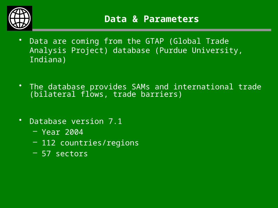
• Data are coming from the GTAP (Global Trade Analysis Project) database (Purdue University, Indiana)

• The database provides SAMs and international trade (bilateral flows, trade barriers)

• Database version 7.1– Year 2004– 112 countries/regions– 57 sectors

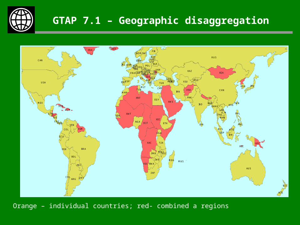
GTAP 7.1 – Geographic disaggregation

RUS

CHN

CAN

USA

BRA

AUS

XWF

XNF

KAZ

XEC

XWS

XAC

IND

ARG

XCF

XEA

MEX

IRN

IDN

ZAF

XSU

PER

ETH

COL

BOL

EGYPAK

XSA

TUR

TZA

NGAVEN

UKR

XSC

MOZ

FRA

ZMB

MAR

SWE

MMR

XNA

CHL

ESP

MDG

BWA

DEU

FIN

THA

POL

JPN

NOR

XSM

XOC

PRY

ZWE

ITA

GBR

NZL

NZL

BLR

VNM

ROU

MYSMYS

PHL

PHL

KGZ

ECU

XER

LAO

UGA

XEF

XCB

XCB

URY

SEN

TUN

KHMXCA

BGR

BGD

GRC

HUN

NIC

AUT

MWI

CZE

LVA

KOR

PRT

IRLLTU

GTM

AZEGEO

EST

PAN

SVK

HRV

DNK

LKA

CHE

NLD

CRI

XEE

BEL

TWN

ARMALB

SVN

XSE

CYP

LUX

MUS

HKG

SGP

MLT

Orange – individual countries; red- combined a regions

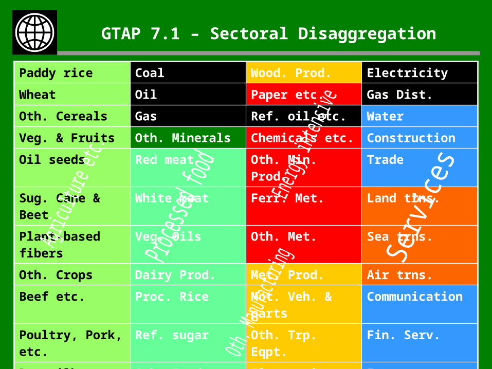
GTAP 7.1 – Sectoral Disaggregation

Paddy rice Coal Wood. Prod. ElectricityWheat Oil Paper etc. Gas Dist.Oth. Cereals Gas Ref. oil etc. WaterVeg. & Fruits Oth. Minerals Chemicals etc. ConstructionOil seeds Red meat Oth. Min. Prod. TradeSug. Cane & Beet White meat Ferr. Met. Land trns.Plant-based fibers Veg. Oils Oth. Met. Sea trns.Oth. Crops Dairy Prod. Met. Prod. Air trns.Beef etc. Proc. Rice Mot. Veh. & parts CommunicationPoultry, Pork, etc. Ref. sugar Oth. Trp. Eqpt. Fin. Serv.Raw milk Oth. Food Electronic Eqpt. InsuranceWool etc. Bev. & Tob. Oth. Mach. & Eqpt. Oth. Bus. Serv.Forestry Textiles Oth. Manu. Recr. & Oth. Serv.

Fishing Clothing Publ. Serv.Leath. Prod. Dwellings

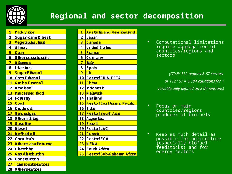
Regional and sector decomposition

• Computational limitations require aggregation of countries/regions and sectors

(GTAP: 112 regions & 57 sectors

or 112* 57 = 6,384 equations for 1

variable only defined on 2 dimensions)

• Focus on main countries/regions producer of biofuels

• Keep as much detail as possible for agriculture (especially biofuel feedstocks) and for energy sectors

1 Paddy rice2 Sugar (cane & beet)3 Vegetables, fruit4 Wheat5 Corn6 Other cereal grains7 Oilseeds8 Livestock9 Sugar Ethanol

10 Corn Ethanol11 Grains Ethanol12 Biodiesel13 Processed food14 Forestry15 Coal16 Crude oil17 Natural gas18 Other mining19 Gasoline20 Diesel21 Refined oil22 Chemicals23 Other manufacturing24 Electricity25 Gas distribution26 Construction27 Transport services28 Other services

1 Australia and New Zealand2 Japan3 Canada4 United States5 France6 Germany7 Italy8 Spain9 UK

10 Rest of EU & EFTA11 China12 Indonesia13 Malaysia14 Thailand15 Rest of East Asia & Pacific16 India17 Rest of South Asia18 Argentina19 Brazil20 Rest of LAC21 Russia22 Rest of ECA23 MENA24 South Africa25 Rest of Sub-Saharan Africa

Key Elasticity Parameters

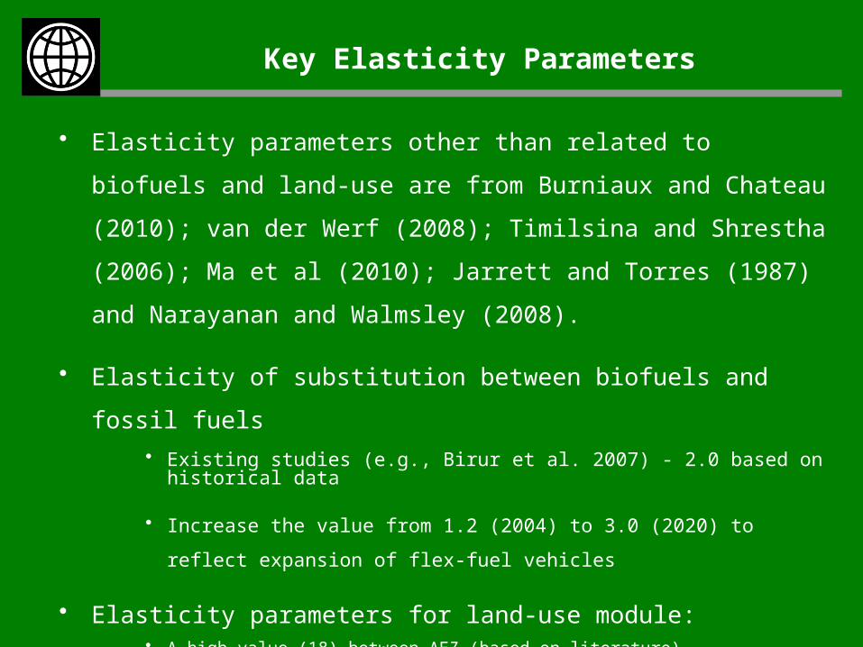
• Elasticity parameters other than related to biofuels and land-use are

from Burniaux and Chateau (2010); van der Werf (2008); Timilsina

and Shrestha (2006); Ma et al (2010); Jarrett and Torres (1987) and

Narayanan and Walmsley (2008).

• Elasticity of substitution between biofuels and fossil fuels

• Existing studies (e.g., Birur et al. 2007) - 2.0 based on historical data

• Increase the value from 1.2 (2004) to 3.0 (2020) to reflect expansion of flex-

fuel vehicles

• Elasticity parameters for land-use module:• A high value (18) between AEZ (based on literature)

• CET elasticity values -- -0.2, -0.5 and -1.0, respectively for top, middle and bottom nests

(Choi, 2004; Hertel et al. 2008)

Single Country Model: Key Features

• Multisector, SAM based general equilibrium model for a country (Thailand, Brazil, Nigeria and Morocco);

• It has two regions: the country and the rest of the world (but assumption small open economy)

• Number of sectors are flexible based on policy questions to be analyzed (for example, in Thailand 187 sectors are aggregated to 21 sectors)

• Deep nested structures for representing the behavior of production and household sectors;

Single Country Model: Difference from other models

• Has detailed representation of the energy sectors and commodities (e.g., coal, crude oil, natural gas, fuel wood, petroleum refinery, gas processing and electricity generation);

• The electricity sector is further divided into seven sub-sectors: hydro; coal-, oil- and gas- fired steam turbine; oil- and gas- fired combined cycle; and diesel fired internal combustion engine;

• Refined petroleum products are divided into three category: gasoline, diesel and others

• Land use and biofuels are explicitly represented to allows modeling of GHG mitigation options in the land use change and forestry sector

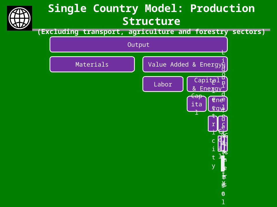
Single Country Model: Production Structure(Excluding transport, agriculture and forestry sectors)

Output

Materials Value Added & Energy

Labor Capital & Energy

Capital

Energy

Electricity

Non-electricity

Coal

Liquid fuel (Petroleum)

Gasoline

Diesel

Others

Gas

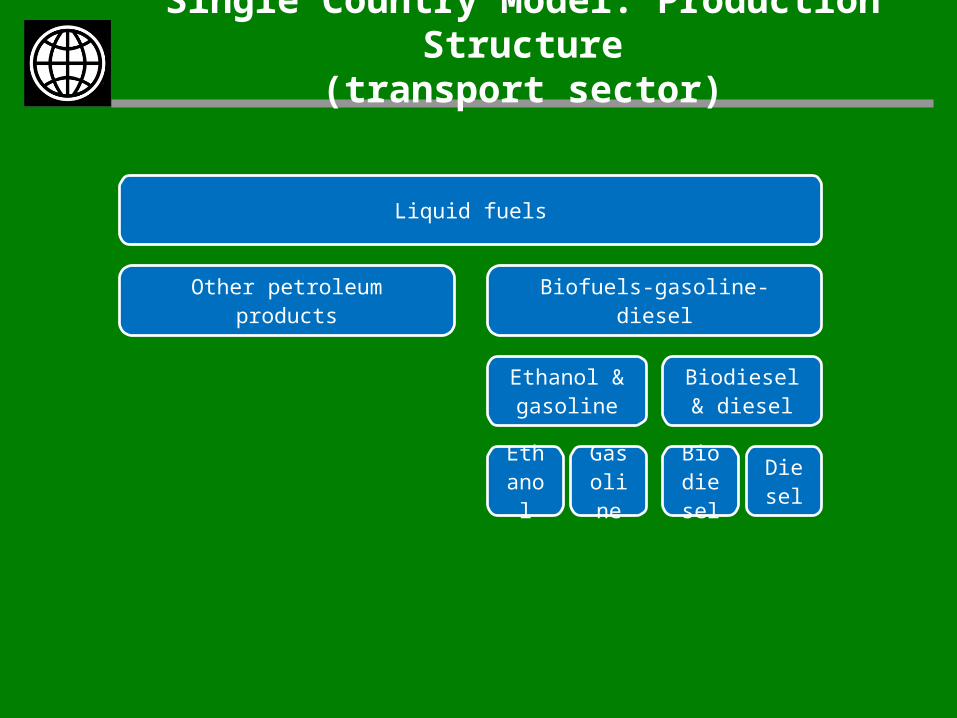
Single Country Model: Production Structure(transport sector)

Liquid fuels

Other petroleum products Biofuels-gasoline-diesel

Ethanol & gasoline

Ethanol

Gasoline

Biodiesel & diesel

Biodiesel

Diesel

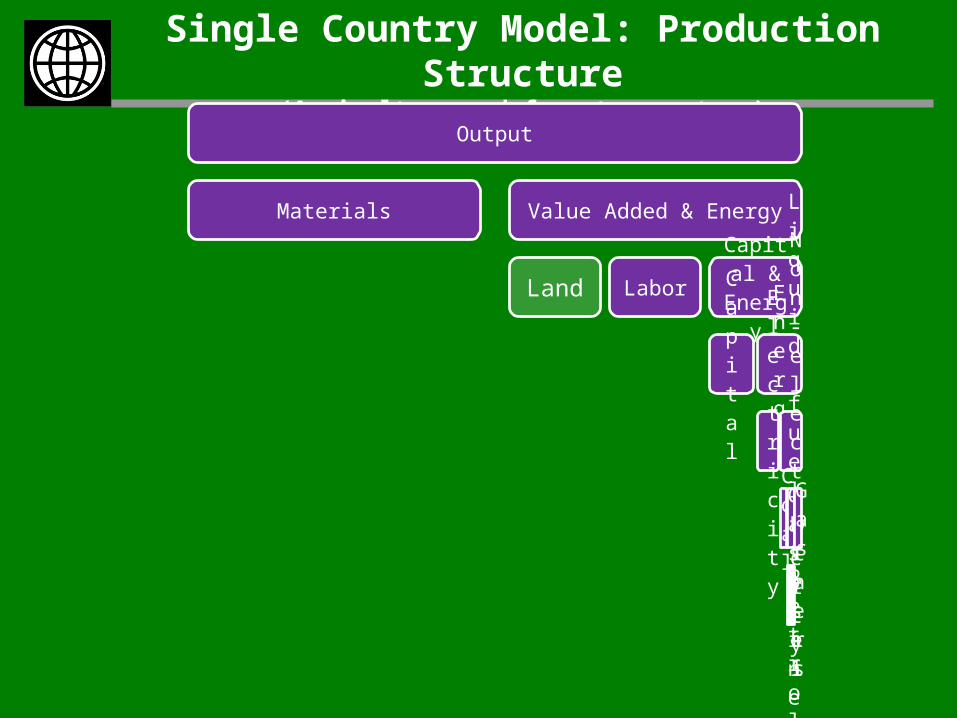
Single Country Model: Production Structure(Agriculture and forestry sectors)

Output

Materials Value Added & Energy

Land Labor

Capital &

EnergyC

apital

Energy

Electricity

Non-electricity

Coal

Liquid fuel (Petroleum)

Gasoline

Diesel

Others

Gas

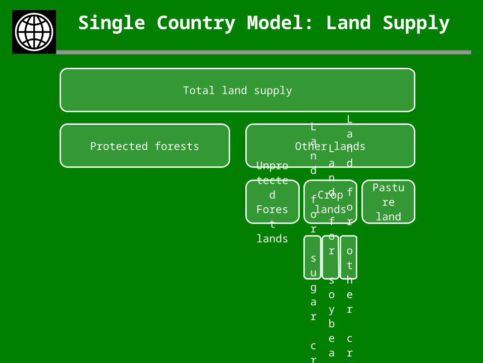
Single Country Model: Land Supply

Total land supply

Protected forests Other lands

UnprotectedForest lands

Crop lands

Land for sugar crop

Land for soybean

Land for other crops

Pasture land

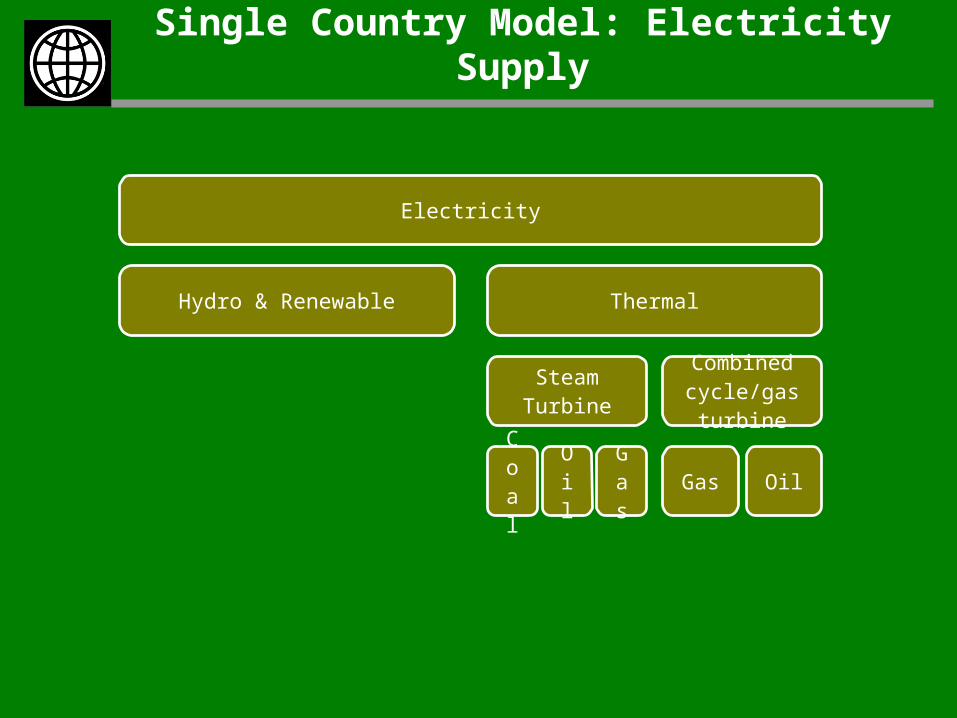
Single Country Model: Electricity Supply

Electricity

Hydro & Renewable Thermal

Steam Turbine

Coal

Oil

Gas

Combined cycle/gas

turbine

Gas Oil

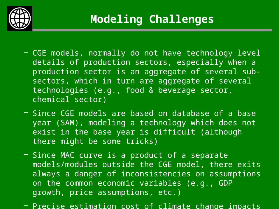
Modeling Challenges

– CGE models, normally do not have technology level details of production sectors, especially when a production sector is an aggregate of several sub-sectors, which in turn are aggregate of several technologies (e.g., food & beverage sector, chemical sector)

– Since CGE models are based on database of a base year (SAM), modeling a technology which does not exist in the base year is difficult (although there might be some tricks)

– Since MAC curve is a product of a separate models/modules outside the CGE model, there exits always a danger of inconsistencies on assumptions on the common economic variables (e.g., GDP growth, price assumptions, etc.)

– Precise estimation cost of climate change impacts is difficult if not impossible.

Govinda R. Timilsina

Sr. Research Economist (Climate Change & Clean Energy)

Development Research Group

The World Bank

1818 H Street, NW

Washington, DC 20433, USA

Room: MC3-451

Mail Drop: MC3-300

Tel: 1 202 473 2767

Fax: 1 202 522 1151

E-mail: gtimilsina@worldbank.org

THANK YOU