GraphPad Guide to Nonlinear Regression - IBCCFfisbio.biof.ufrj.br/.../bioEstatistica/90_top_especiais/nonlin.pdf · The GraphPad Guide to Nonlinear Regression The GraphPad Guide to

The GraphPad

Guide to

NonlinearRegression

Dr. Harvey MotulskyPresident, Graphpad SoftwareApril 1996

The GraphPad Guide to Nonlinear Regression The GraphPad Guide to Nonlinear Regression 2

This booklet was published by GraphPad Software Inc., thecreators of GraphPad Prism® – your complete solution forscientific graphics, curve fitting and statistics.

Copyright © 1995-96 by GraphPad Software, Inc. All rights reserved.

You may obtain additional copies of this booklet by downloading thedocument from the internet at http://www.graphpad.com. You may alsoorder additional copies from GraphPad Software.

Companion booklets on radioligand binding and statistical comparisonsmay be available by the time you read this.

GraphPad Prism is a registered trademark of GraphPad Software, Inc.

To contact GraphPad Software:Phone 800-388-4723 (US only) or 619-457-3909

Fax (USA) 619-457-8141

Email [email protected] [email protected]

World Wide Web http://www.graphpad.com

Mail GraphPad Software, Inc.10855 Sorrento Valley Road #203San Diego, CA 92121 USA

INTRODUCTION TO NONLINEAR REGRESSION................................3Why you should use nonlinear regression ..............................................3

Linear regression of transformed data is less accurate ............................................ 3Don't relegate scientific decisions to a computer program ..................................... 4The results of polynomial regression are often impossible to interpret scientifically 4Cubic spline is not a data analysis method ............................................................ 4

Terminology ........................................................................................... 4How nonlinear regression works ............................................................ 5

Comparison of linear and nonlinear regression...................................................... 5Iterations in nonlinear regression .......................................................................... 5

Decisions to make when using nonlinear regression ............................... 5Choose a model ................................................................................................... 5Prepare data for nonlinear regression .................................................................... 5Estimate initial values ........................................................................................... 6Constants ............................................................................................................. 6Weighting ............................................................................................................ 6Average replicates?............................................................................................... 7

INTERPRETING NONLINEAR REGRESSION RESULTS..........................8Assumptions of nonlinear regression .......................................................8Variables, standard errors, and confidence intervals ................................ 8Sum-of-squares, sy.x, and R2 .....................................................................8Residuals and the runs test ......................................................................9How to tell if the nonlinear regression fit is any good ............................. 9

Did the fit converge on a solution? ....................................................................... 9Does the curve come close to the points? ........................................................... 10Are the results scientifically plausible? ................................................................ 10Do the data systematically deviate from the curve? ............................................. 10Are the confidence intervals wide? ..................................................................... 10Is the fit a local minimum? ................................................................................. 11

What to do when the fit is no good? .....................................................12Comparing two equations .....................................................................13

How the F test works.......................................................................................... 13Example............................................................................................................. 14

Comparing fits to two data sets ............................................................. 141. Compare the results of repeated experiments. ................................................. 142. Compare the results within one experiment. Simple approach. ........................ 153. Compare the results within one experiment. More complicated approach. ...... 15Advantages and disadvantages of the three methods ........................................... 16

GRAPHPAD PRISM .............................................................................17


Introduction to nonlinear regression

Nonlinear regression is a powerful tool for analyzing scientific data,especially in pharmacology and physiology. The goal of nonlinear regre s-sion is to fit a model to your data. The program finds the best-fit values ofthe variables in the model (perhaps rate constants, affinities, receptornumber, etc.) which you can interpret scientifically. In most cases, theprimary goal is to obtain those values and a secondary goal is to draw agraph of the fit curve.

In some situations, you only goal is to draw a curve. You don't care aboutmodels or equations, and don't want to obtain best-fit values. You justwant a smooth curve through your points either for artistic reasons or touse as a standard curve. You may still use nonlinear regression in thesesituations, or you may use these alternatives:

• Polynomial regression.

• Cubic spline or LOWESS curve.

• A program that fits your data to thousands of equations and picksthe best.

This chapter (and the next two) assumes that your goal is primarily toobtain the best-fit values of the variables – to fit a model to your data.

Why you should use nonlinear regression

Linear regression of transformed data is less accurate

Before the age of microcomputers, nonlinear regression was not readilyavailable to most scientists. Instead, scientists transformed their data tomake a linear graph, and then analyzed the transformed data with linearregression. Examples include Lineweaver-Burke plots of enzyme kineticdata, Scatchard plots of binding data, and logarithmic plots of kinetic data.

These methods are outdated, and should not be used to analyze data. Theproblem is that the linear transformation distorts the experimental error.Linear regression assumes that the scatter of points around the line followsa Gaussian distribution, and that the standard devia tion is the same at

every value of X. These assumptions are usually not true with the tran s-formed data. A second problem is that some transformations alter therelationship between X and Y. For example, in a Scatchard plot thevalue of X (bound) is used to calculate Y (bound/free), and this violatesthe assumptions of linear regression.

Since the assumptions of linear regression are violated, the results oflinear regression are incorrect. The values derived from the slope andintercept of the regression line are not the most accurate determinationsof the variables in the model. Considering all the time and effort you putinto collecting data, you want to use the best possible analysis tec h-nique. Nonlinear regression produces the most accurate results.

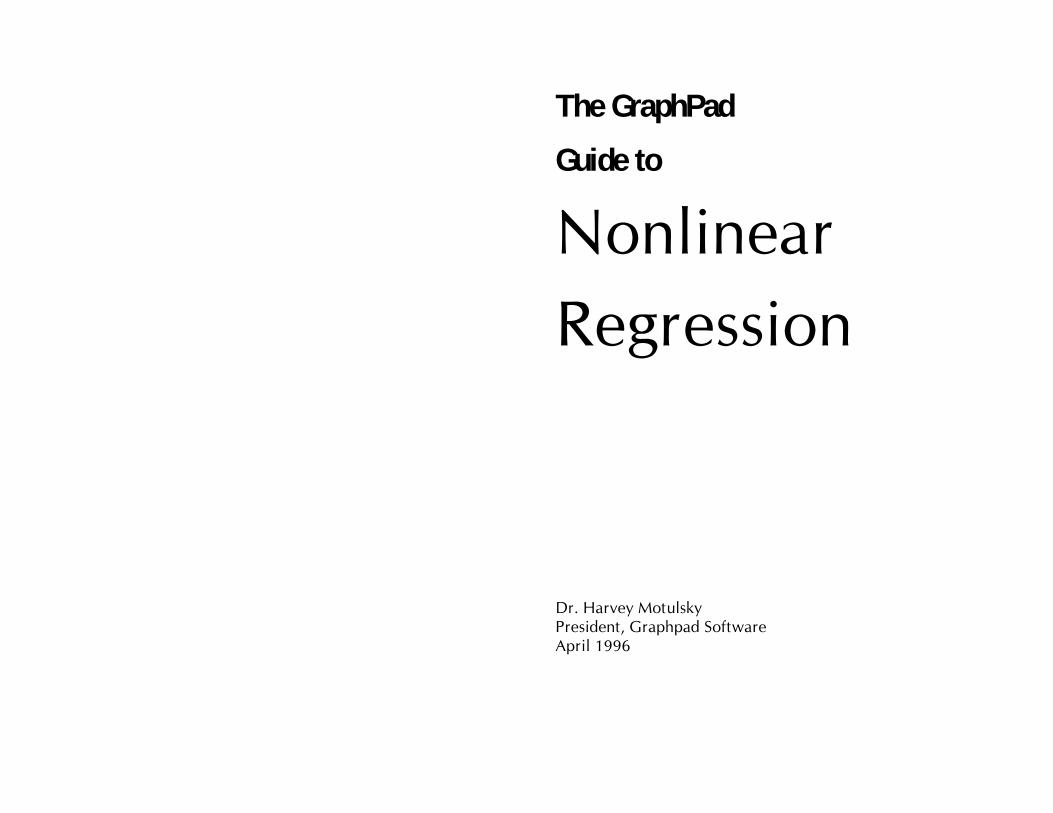
This figure shows the problem of transforming data. The left panelshows data that follows a rectangular hyperbola (binding isotherm). Theright panel is a Scatchard plot of the same data. The solid curve on theleft was determined by nonlinear regression. The solid line on the rightshows how that same curve would look after a Scatchard transform a-tion. The dotted line shows the linear regression fit of the transformeddata. The transformation amplified and distorted the scatter, and thus thelinear regression fit does not yield the most accurate values for B max andKd.

[Ligand]S

pec

ific

Bin

din

g

0 50 100 1500

10

20

30

40

50

Bound

Bo

un

d/F

ree

0 10 20 30 40 50 600

1

2

Transformations can be very useful when used appropriately. Whenanalyzing data, follow these rules:

• You should transform your data when the transformation makesthe variability more consistent and more Gaussian.

• You should not transform data when the transformation makes thevariability less consistent and less Gaussian.


• You should not perform transforms (such as the Scatchard trans form)that destroy the relationship between X and Y.

• You should not transform the data merely to make it linear. Sincenonlinear regression is easy, there is no reason to force your datainto a linear form.

Although it is usually inappropriate to analyze transformed data, it is oftenhelpful to display data after a linear transform. Many people find it easierto visually interpret transformed data. This makes sense because the hu -man eye and brain evolved to detect edges (lines) — not to detect rectan -gular hyperbolas or exponential decay curves. Even if you analyze yourdata with nonlinear regression, it may make sense to display transformeddata.

Don't relegate scientific decisions to a computer program

The goal of nonlinear regression is to fit a model to your data. The pr o-gram finds the best-fit values of the variables in the model (perhaps rateconstants, affinities, receptor number, etc.) which you can interpretscientifically. Choosing a model is a scientific decision. You should baseyour choice on your understanding of chemistry or physiology (or gene t-ics, etc.). The choice should not be based solely on the shape of thegraph.

Some programs automatically fit data to hundreds or thousands of equ a-tions and then present you with the equation(s) that fit the data best.Using such a program is appealing because it frees you from the need tochoose an equation. The problem is that the program has no understan d-ing of the scientific context of you experiment. The equations that fit thedata best are unlikely to correspond to scientifically meaningful models.You will not be able to interpret the best-fit values of the variables, andthe results are unlikely to be useful for data anal ysis.

This kind of approach is very useful in three situations:

• Your only goal is to plot an attractive curve.

• You wish to create a standard curve for interpolating unknown va l-ues.

• You need an equation to use within a computer simulation.

In all three situations, it doesn't matter whether the equation corr e-sponds to a biological, chemical or physical model. What matters is thatthe equation accurately predict Y from X within the range of your data.

This approach can be useful in some situations. Don't use it when thegoal of curve fitting is to fit the data to a model based on chemical,physical, or biological principles. Don't use a computer program toavoid making a scientific decision.

The results of polynomial regression are often impossible to interpretscientifically

Beware of the term "curve fitting". The term is often used to refer not tononlinear regression, but rather to polynomial regression. This methodfits data to a polynomial equation: Y=A + BX + CX 2 + DX3..... Pro-grammers prefer polynomial regression, because it is so much easier toprogram. That's why it is built in to so many spreadsheet and graphicsprograms. But few biological or chemical models are described bypolynomial equations, so polynomial regression is of limited usefulnessto scientists.

Cubic spline is not a data analysis method

Cubic spline curves are smooth curves that go through every data point.In some cases, a cubic spline curve can look attractive on a graph andwork well as a standard curve for interpolation. The curve does notcorrespond to any equation (or rather the equation differs for every pairof points) so cubic spline is not useful in data analysis.

TerminologyA model is a formal presentation of a chemical or physiological idea. Tobe useful for nonlinear regression, the model must be expressed as anequation that defines Y, the outcome you measure, as a function of Xand one or more variables that you want to fit. We use the term variableto refer to the terms in the equation you want to fit. In the context ofnonlinear regression, the term variable does not refer to X and Y. Someprograms and books use the word parameters rather than variables.


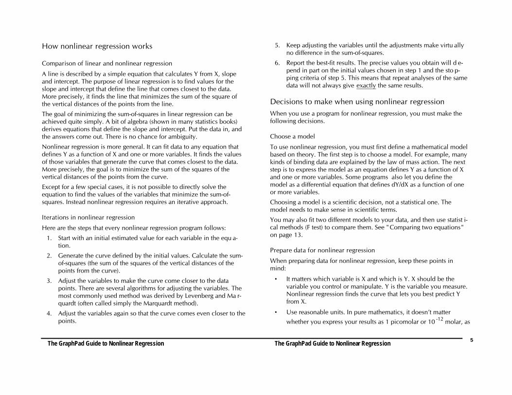
How nonlinear regression works

Comparison of linear and nonlinear regression

A line is described by a simple equation that calculates Y from X, slopeand intercept. The purpose of linear regression is to find values for theslope and intercept that define the line that comes closest to the data.More precisely, it finds the line that minimizes the sum of the square ofthe vertical distances of the points from the line.

The goal of minimizing the sum-of-squares in linear regression can beachieved quite simply. A bit of algebra (shown in many statistics books)derives equations that define the slope and intercept. Put the data in, andthe answers come out. There is no chance for ambiguity.

Nonlinear regression is more general. It can fit data to any equation thatdefines Y as a function of X and one or more variables. It finds the valuesof those variables that generate the curve that comes closest to the data.More precisely, the goal is to minimize the sum of the squares of thevertical distances of the points from the curve.

Except for a few special cases, it is not possible to directly solve theequation to find the values of the variables that minimize the sum-of-squares. Instead nonlinear regression requires an iterative approach.

Iterations in nonlinear regression

Here are the steps that every nonlinear regression program follows:

1. Start with an initial estimated value for each variable in the equ a-tion.

2. Generate the curve defined by the initial values. Calculate the sum-of-squares (the sum of the squares of the vertical distances of thepoints from the curve).

3. Adjust the variables to make the curve come closer to the datapoints. There are several algorithms for adjusting the variables. Themost commonly used method was derived by Levenberg and Ma r-quardt (often called simply the Marquardt method).

4. Adjust the variables again so that the curve comes even closer to thepoints.

5. Keep adjusting the variables until the adjustments make virtu allyno difference in the sum-of-squares.

6. Report the best-fit results. The precise values you obtain will d e-pend in part on the initial values chosen in step 1 and the sto p-ping criteria of step 5. This means that repeat analyses of the samedata will not always give exactly the same results.

Decisions to make when using nonlinear regressionWhen you use a program for nonlinear regression, you must make thefollowing decisions.

Choose a model

To use nonlinear regression, you must first define a mathematical modelbased on theory. The first step is to choose a model. For example, manykinds of binding data are explained by the law of mass action. The nextstep is to express the model as an equation defines Y as a function of Xand one or more variables. Some programs also let you define themodel as a differential equation that defines dY/dX as a function of oneor more variables.

Choosing a model is a scientific decision, not a statistical one. Themodel needs to make sense in scientific terms.

You may also fit two different models to your data, and then use statist i-cal methods (F test) to compare them. See " Comparing two equations"on page 13.

Prepare data for nonlinear regression

When preparing data for nonlinear regression, keep these points inmind:

• It matters which variable is X and which is Y. X should be thevariable you control or manipulate. Y is the variable you measure.Nonlinear regression finds the curve that lets you best predict Yfrom X.

• Use reasonable units. In pure mathematics, it doesn’t matterwhether you express your results as 1 picomolar or 10 -12 molar, as


1 nanovolt or 10-9 volts. When computers do the calculating, ho w-ever, it can matter. Calculation problems such as round off errorsare far more likely when the values are very high or very low. Werecommend that you scale your data to avoid values less than 10 -4

or greater than 104.

• Don’t smooth. You lose information when you smooth data, andthis won’t get you a better fit.

• If you are fitting data to a sigmoidal dose-response or competitivebinding curve, enter the X values as the logarithm of concentration,rather than the concentration itself.

Estimate initial values

Nonlinear regression is an iterative procedure. The program must startwith estimated values for each variable that are in the right “ball park” —say within a factor of five of the actual value. It then adjusts these initialvalues to improve the fit. It then adjusts the values again and again untilthe improvement is tiny.

Some programs automatically provide initial values automatically. Withother programs, you must enter the values manually. If you have “clean”data that clearly define a curve, then it usually doesn't matter if the initialvalues are fairly far from the correct values. You'll get the same answer nomatter what initial values you use, unless the initial values are very farfrom correct.

Initial values matter more when your data have a lot of scatter, don't spana large enough range of X values to define a full curve, or don't re ally fitthe model. In these cases, you may get different answers depend ing onwhich initial values you use. See “ Is the fit a local minimum?” on page11.

You'll find it easy to estimate initial values if you have looked at a graphof the data, and understand the model and what all the variables mean.Remember, you just need an estimate. It doesn't have to be very accurate.If you are having problems estimating an initial value:

• Check that you have chosen a model that makes scientific sense.

• Make sure you understand what each variable in the equationmeans.

• Put away your data, and spend an hour or two generating curvesusing the model. Change the variables one at a time, and see howthey influence the shape of the curve.

Constants

You don't have to fit every variable in the equation. In many situations itmakes sense to fix some of the variables to constant values. For exa m-ple, you might want to define the bottom plateau of a dose-responsecurve or an exponential decay curve to equal zero.

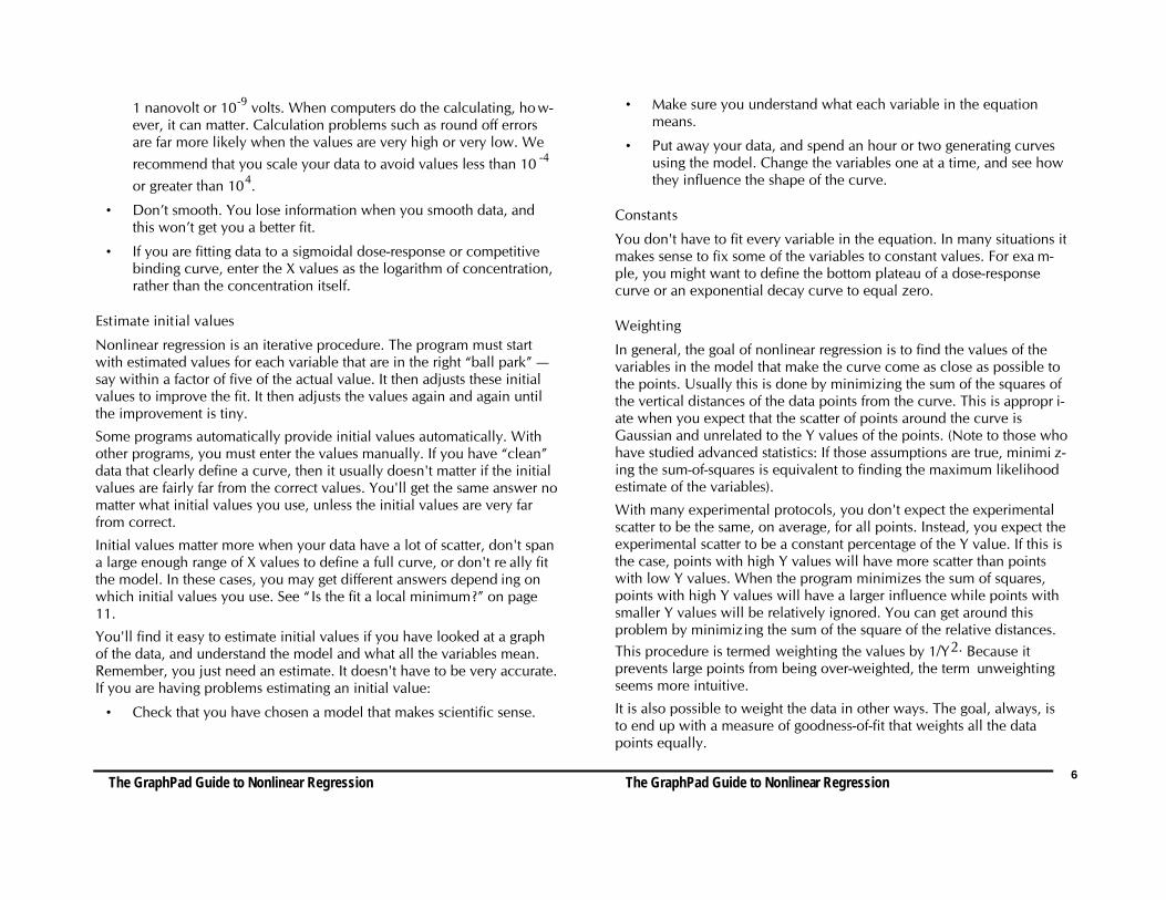
Weighting

In general, the goal of nonlinear regression is to find the values of thevariables in the model that make the curve come as close as possible tothe points. Usually this is done by minimizing the sum of the squares ofthe vertical distances of the data points from the curve. This is appropr i-ate when you expect that the scatter of points around the curve isGaussian and unrelated to the Y values of the points. (Note to those whohave studied advanced statistics: If those assumptions are true, minimi z-ing the sum-of-squares is equivalent to finding the maximum likelihoodestimate of the variables).

With many experimental protocols, you don't expect the experimentalscatter to be the same, on average, for all points. Instead, you expect theexperimental scatter to be a constant percentage of the Y value. If this isthe case, points with high Y values will have more scatter than pointswith low Y values. When the program minimizes the sum of squares,points with high Y values will have a larger influence while points withsmaller Y values will be relatively ignored. You can get around thisproblem by minimizing the sum of the square of the relative distances.This procedure is termed weighting the values by 1/Y2. Because itprevents large points from being over-weighted, the term unweightingseems more intuitive.

It is also possible to weight the data in other ways. The goal, always, isto end up with a measure of goodness-of-fit that weights all the datapoints equally.


Average replicates?

If you collected replicate Y values at every value of X, there are two waysto analyze the data:

• Treats each replicate as a separate point.

• Average the replicate Y values, and treat the mean as a single point.

Deciding which approach to use can be difficult.

The advantage of the first approach is that you have more data points andthus more degrees of freedom. However, you should only use that a p-proach when the experimental error of each replicate is no more closelyrelated to the other replicates than to other data points. Here are twoexamples where you should analyze each replicate:

• You are doing a radioligand binding experiment. All the data wereobtained from one tissue preparation and each replicate was dete r-mined from a separate incubation (separate test tube). The sourcesof experimental error are the same for each tube. If one value ha p-pens to be a bit high, there is no reason to expect the other repl i-cates to be high as well.

• You are doing an electrophysiology study. You apply a voltageacross a cell membrane and measure conductance. Each data pointwas obtained from a separate cell. The possible sources of exper i-mental error are independent for each cell. If one cell happens tohave a high conductance, there is no reason to expect the replicatecells (those that you apply the same voltage to) to also have highconductance.

You should not treat each replicate as a separate point when the exper i-mental error of the replicates are related. You should average the repl i-cates instead, and analyze the averages. Here are two examples whereyou should average the replicates:

• The experiment was only performed with a single replicate at eachvalue of X, and you measure radioactivity as Y. Each tube iscounted three times, and the three counts are treated as replicates.Any experimental error while conducting the experiment wouldappear in all the replicates. The replicates are not independent.

• The experiment is a dose-response curve. At each dose, you use adifferent animal but measure the response three times. The threemeasurements are not independent. If an animal happens to r e-spond more than the others, that will affect all the replicates. Thereplicates are not independent.


Interpreting results

Assumptions of nonlinear regressionThe results of nonlinear regression are meaningful only if these assum p-tions are true (or nearly true):

• The model is correct. Nonlinear regression adjusts the variables inthe equation you chose to minimize the sum-of-squares. It does notattempt to find a better equation.

• The variability of values around the curve follow a Gaussian dis tri-bution. Even though no biological variable follows a Gaussian dis -tribution exactly, it is sufficient that the variation be approxi matelyGaussian.

• The SD of the variability is the same everywhere, regardless of thevalue of X. The assumption is termed homoscedasticity . If the SD isnot constant but rather is proportional to the value of Y, you shouldweight the data to minimize the sum-of-squares of the rel ative dis-tances.

• The model assumes that you know X exactly. This is rarely the case,but it is sufficient to assume that any impreci sion in measuring X isvery small compared to the variability in Y.

• The errors are independent. The deviation of each value from thecurve should be random, and should not be correlated with the de-viation of the previous or next point. If there is any carryover fromone sample to the next, this assumption will be violated.

Variables, standard errors, and confidence intervalsAlong with the best-fit value of each variable in the equation, nonlinearregression programs usually report its standard error and 95% confidenceinterval.

By itself, the standard error is difficult to interpret. It is used to calculatethe 95% confidence interval, which is easier to interpret.

This is what the CI is supposed to mean: If all the assumptions of no n-linear regression are true, there is a 95% chance that the true value ofthe variable lies within the interval. More precisely, if you performnonlinear regression many times (on different data sets) you expect theconfidence interval to include the true value 95% of the time, but toexclude the true value the other 5% of the time.

Three factors can make the confidence interval too narrow:

• The CI is based only on the scatter of data points around the curvewithin this one experiment . If you repeat the experiment manytimes, the scatter between the results is likely to be greater thanpredicted from the CI based on one experiment.

• The CI can only be interpreted if you accept the assumptions ofnonlinear regression. See "Assumptions of nonlinear regression"on page 8.

• The confidence intervals from linear regression are calculatedusing straightforward mathematical methods. If you accept the a s-sumptions of linear regression, then you can interpret the 95% CIof slope and intercept quite rigorously. It is not straightforward tocalculate the 95% CI of variables from nonlinear regression –mathematical shortcuts are needed. These shortcut intervals(reported by most programs) are sometimes referred to as asym p-totic confidence intervals. In some cases these intervals can be toonarrow (too optimistic).

Because of these problems, you shouldn't interpret the confidenceintervals too rigorously. Rather than focusing on the CI reported fromanalysis of this one experiment, you should repeat the experimentseveral times.

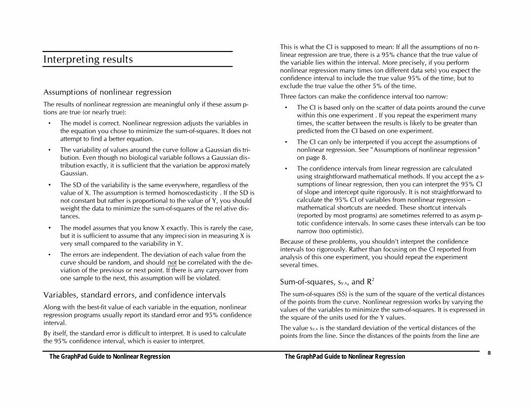
Sum-of-squares, sy.x, and R2

The sum-of-squares (SS) is the sum of the square of the vertical distancesof the points from the curve. Nonlinear regression works by varying thevalues of the variables to minimize the sum-of-squares. It is expressed inthe square of the units used for the Y values.

The value sy.x is the standard deviation of the vertical distances of thepoints from the line. Since the distances of the points from the line are


called residuals, sy.x is the standard deviation of the residuals. Its value isexpressed in the same units as Y.

The value R2 is a measure of goodness of fit. It is a fraction between 0.0and 1.0, and has no units. When R 2 equals 0.0, the best-fit curve fits thedata no better than a horizontal line going through the mean of all Y val -ues. In this case, knowing X does not help you predict Y. When R 2=1.0,all points lie exactly on the curve with no scatter. If you know X you cancalculate Y exactly.

You can think of R2 as the fraction of the total variance of Y that is ex -plained by the model (equation). Mathematically, it is defined by thisequation: R2 =1.0 - SSreg/Sstot, where SSreg is the sum-of-squares of the pintsfrom the regression curve and SStot is the sum-of-squares of the distancesof the points from a horizontal line where Y equals the mean of all thedata points.

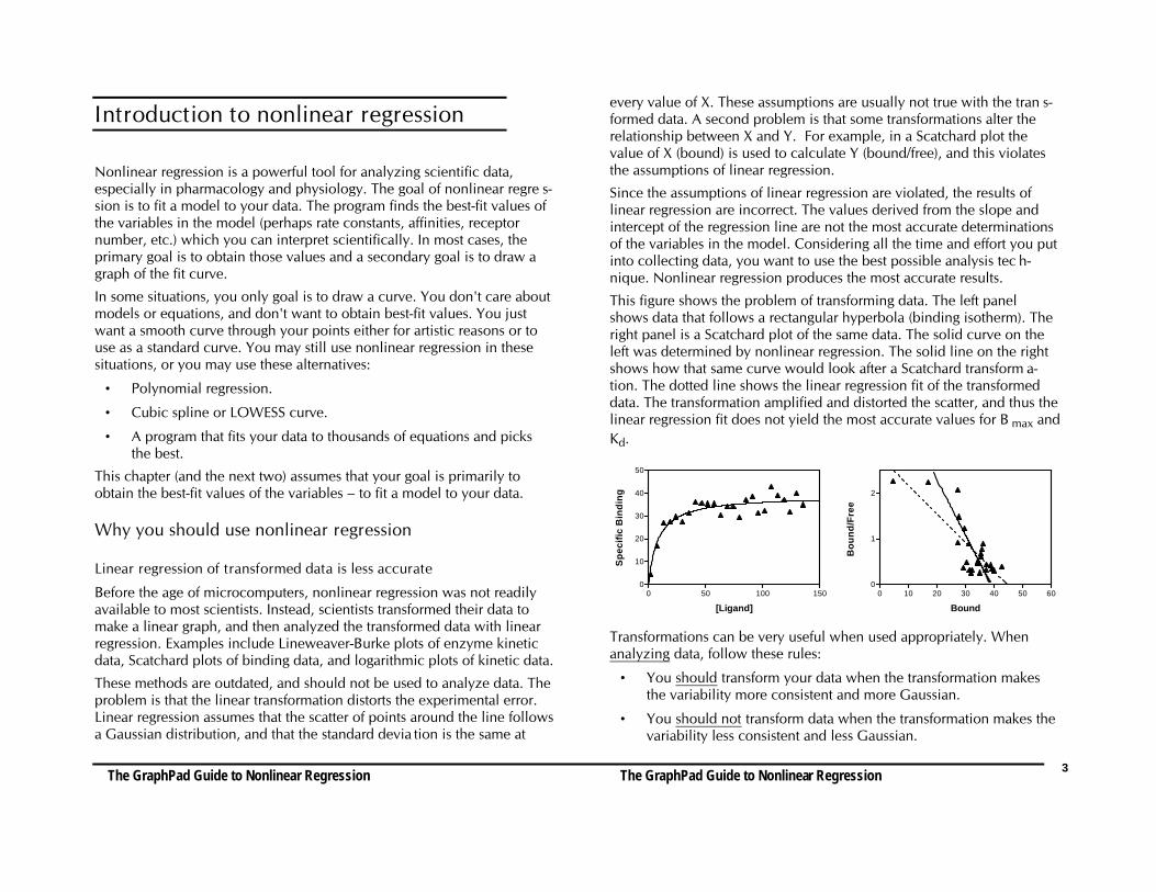
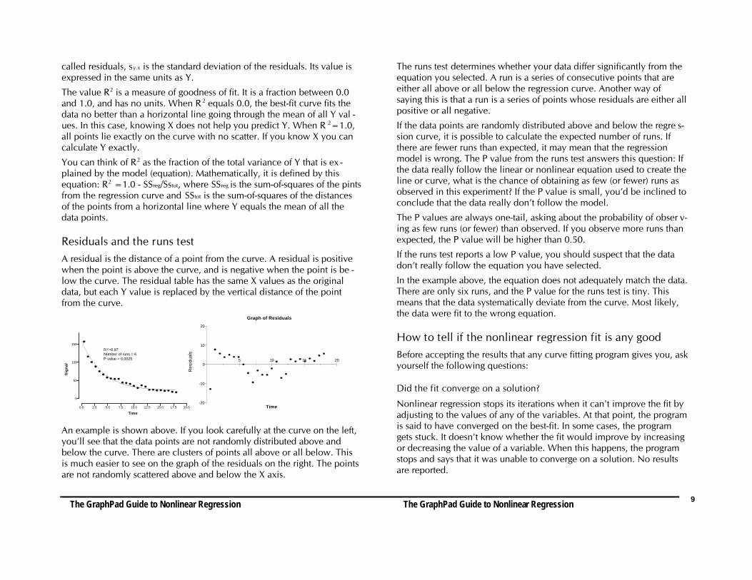
Residuals and the runs testA residual is the distance of a point from the curve. A residual is positivewhen the point is above the curve, and is negative when the point is be -low the curve. The residual table has the same X values as the originaldata, but each Y value is replaced by the vertical distance of the pointfrom the curve.

Time

Sig

nal

0.0 2.5 5.0 7.5 10.0 12.5 15.0 17.5 20.0

0

50

100

150

R2=0.97Number of runs = 6P value = 0.0025

Graph of Residuals

Time

Res

idua

ls

5 10 15 20

-20

-10

0

10

20

An example is shown above. If you look carefully at the curve on the left,you’ll see that the data points are not randomly distributed above andbelow the curve. There are clusters of points all above or all below. Thisis much easier to see on the graph of the residuals on the right. The pointsare not randomly scattered above and below the X axis.

The runs test determines whether your data differ significantly from theequation you selected. A run is a series of consecutive points that areeither all above or all below the regression curve. Another way ofsaying this is that a run is a series of points whose residuals are either allpositive or all negative.

If the data points are randomly distributed above and below the regre s-sion curve, it is possible to calculate the expected number of runs. Ifthere are fewer runs than expected, it may mean that the regressionmodel is wrong. The P value from the runs test answers this question: Ifthe data really follow the linear or nonlinear equation used to create theline or curve, what is the chance of obtaining as few (or fewer) runs asobserved in this experiment? If the P value is small, you’d be inclined toconclude that the data really don’t follow the model.

The P values are always one-tail, asking about the probability of obser v-ing as few runs (or fewer) than observed. If you observe more runs thanexpected, the P value will be higher than 0.50.

If the runs test reports a low P value, you should suspect that the datadon’t really follow the equation you have selected.

In the example above, the equation does not adequately match the data.There are only six runs, and the P value for the runs test is tiny. Thismeans that the data systematically deviate from the curve. Most likely,the data were fit to the wrong equation.

How to tell if the nonlinear regression fit is any goodBefore accepting the results that any curve fitting program gives you, askyourself the following questions:

Did the fit converge on a solution?

Nonlinear regression stops its iterations when it can't improve the fit byadjusting to the values of any of the variables. At that point, the programis said to have converged on the best-fit. In some cases, the programgets stuck. It doesn't know whether the fit would improve by increasingor decreasing the value of a variable. When this happens, the programstops and says that it was unable to converge on a solution. No resultsare reported.


Does the curve come close to the points?

In rare cases, the fit may be far from the data points. This may happen, forexample, if you picked the wrong equation. Look at the graph to makesure this didn’t happen.

Also look at the R2 value. It is the fraction of the overall variance in Y thatis “explained” by the model. See “R” on page 8. If R2 is low, the curvedoes not come close to the points. If R 2 is high, you can conclude that thecurve comes closer to the points than would a horizontal line through themean Y value. But don’t over interpret a high R 2 . It does not mean thatyou have chosen the equation that best de scribes the data. It also does notmean that the fit is unique — other values of the variables may generate acurve that fits just as well.

Are the results scientifically plausible?

A computer program can only follow a procedure to fit a curve. It is up toyou to figure out what they mean. Before accepting the results, ask you r-self if the results make any sense.

The mathematics of curve fitting sometimes yields results that make noscientific sense. For example with noisy or incomplete data, nonlinearregression can calculate negative rate constants, fractions greater than 1.0,and negative Kd values. Its up to you to realize that these are no nsense.

If the results make no scientific sense, you should conclude that the fit isno good, regardless of R2 and regardless of how close the curve comes tothe points. Try a simpler equation, or try fixing some variables to con stantvalues.

Also check that the best-fit values of the variables make sense in light ofthe range of the data. Don’t trust the results if the top plateau of a sig moidcurve is far larger than the highest data point. Don’t trust the results if anEC50 value is not within the range of your X values.

Do the data systematically deviate from the curve?

If the data really follow the model described by your equation, the datapoints should randomly bounce above and below the curve. The dis tanceof the points from the curve should also be random, and not be re lated tothe value of X.

The best way to look for systematic deviations of the points from thecurve is to inspect a graph of the residuals and to look at the runs test.See “Residuals and the runs test“ on page 9. With a good fit, the re-siduals should be randomly distributed between positive and negativevalues and the P value from the runs test will be high.

If the runs test reports a low P value, you should suspect that the datadon’t really follow the equation you have selected.

Are the confidence intervals wide?

Most nonlinear regression programs report the standard error of eachvariable, and its 95% confidence interval. You can be approximately95% sure that the true value of the variable lies within the confidenceinterval.

The confidence interval will be very wide (i.e. the standard error will bevery large) when the fit is not unique. This means that curves generatedfrom other values of the variables would fit nearly as well.

Confidence intervals are wide in these circumstances:

• You have not collected data over a wide enough range of X va l-ues. See the first example below.

• You have not collected data in an important part of the curve. Seethe second example below.

• The data are very scattered.

• The equation contains redundant variables. For example, the co n-fidence intervals would be very wide if you fit this equation: Y =A + B + C*X. This equation describes a line, but the intercept isdefined by the sum of A plus B. There is no way for the programto know how to apportion the value between A and B, so bothwill have very wide confidence intervals.


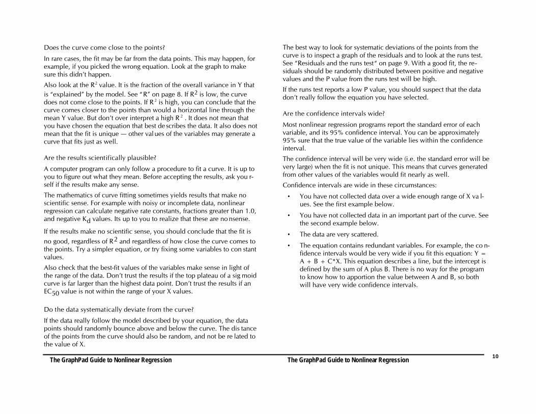
Example 1. Data not collected over a wide range of X.

log[Dose]

Per

cen

t R

esp

on

se

0

50

100

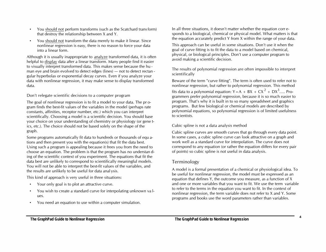
Fit to sigmoidal curveR2=0.9999

This best-fit dose response curve has wide confidence intervals. The 95%CI for the EC50 extends over six orders of magnitude!

The explanation is simple. The data were fit to a sigmoidal equation withfour variables: the top plateau, the bottom plateau, the slope, and the EC 50

(the log[Dose] when response=50%). But the data do not form plateaus ateither the top or the bottom, so best-fit values for the plateaus are veryuncertain. The information is simply not in the data. Since the data do notclearly define zero and one hundred, the value for the EC 50 is very impre-cise. The program indicates this by reporting large standard errors andwide confidence intervals. The fit is not unique. You could find othervalues of the variables that fit the data equally well.

In this example, it might make scientific sense to set the bottom plateau to0% and the top plateau to 100% (if the plateaus were defined by othercontrols not shown on the graph). If you did this, the equation would fitfine and the confidence interval would be narrow.

Note that the problem with the fit is not obvious by inspecting a graph,because the curve goes very close to the points. The value of R 2 (0.9999)is also not helpful. That value just tells you that the curve comes close tothe points, but does not tell you whether the fit is unique.

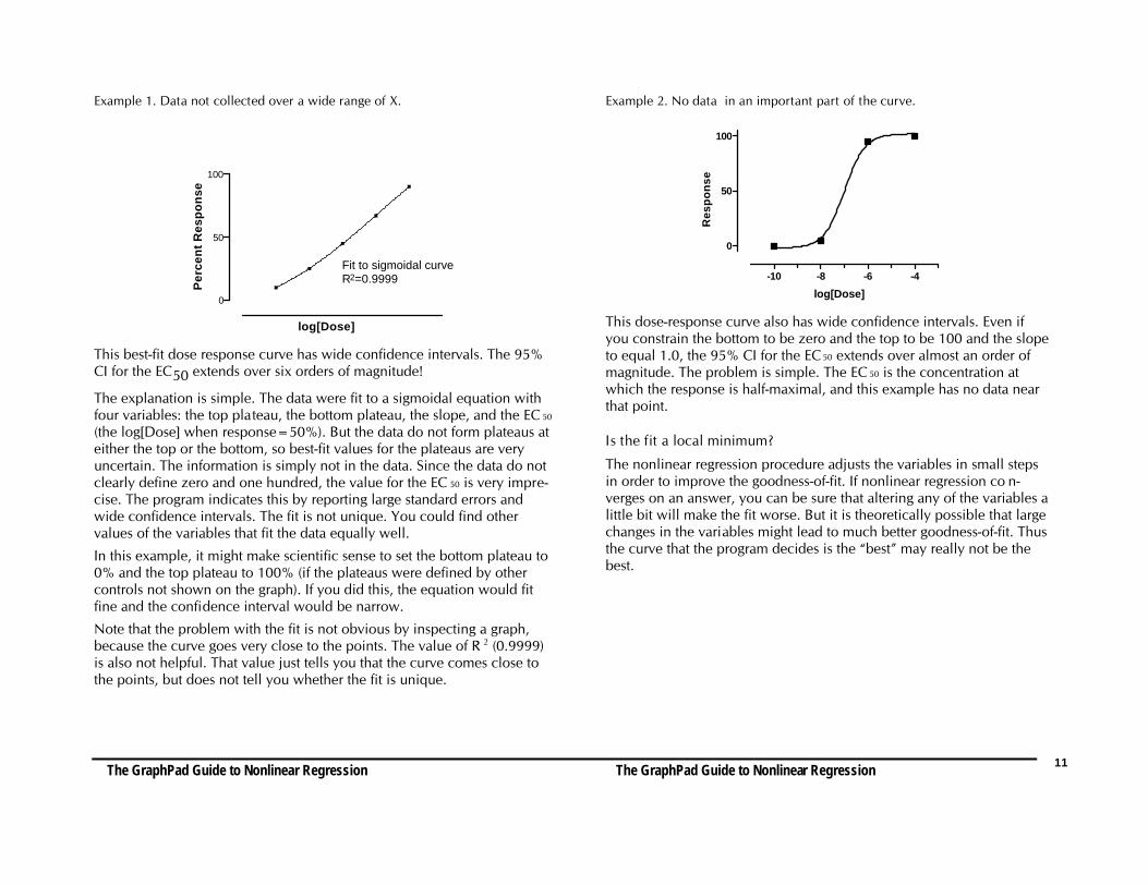
Example 2. No data in an important part of the curve.

log[Dose]

Res

po

nse

-10 -8 -6 -4

0

50

100

This dose-response curve also has wide confidence intervals. Even ifyou constrain the bottom to be zero and the top to be 100 and the slopeto equal 1.0, the 95% CI for the EC 50 extends over almost an order ofmagnitude. The problem is simple. The EC 50 is the concentration atwhich the response is half-maximal, and this example has no data nearthat point.

Is the fit a local minimum?

The nonlinear regression procedure adjusts the variables in small stepsin order to improve the goodness-of-fit. If nonlinear regression co n-verges on an answer, you can be sure that altering any of the variables alittle bit will make the fit worse. But it is theoretically possible that largechanges in the variables might lead to much better goodness-of-fit. Thusthe curve that the program decides is the “best” may really not be thebest.


Value of Variable

SU

M-O

F-S

QU

AR

ES

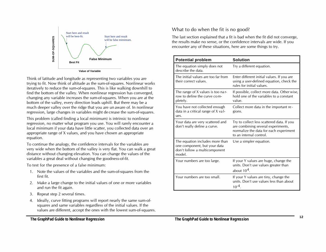
Best FitFalse Minimum

Start here and result will be false mimimum.

Start here and result will be best-fit.

Think of latitude and longitude as representing two variables you aretrying to fit. Now think of altitude as the sum-of-squares. Nonlinear worksiteratively to reduce the sum-of-squares. This is like walking downhill tofind the bottom of the valley. When nonlinear regression has converged,changing any variable increases the sum-of-squares. When you are at thebottom of the valley, every direction leads uphill. But there may be amuch deeper valley over the ridge that you are un aware of. In nonlinearregression, large changes in variables might de crease the sum-of-squares.

This problem (called finding a local minimum) is intrinsic to nonlinearregression, no matter what program you use. You will rarely encounter alocal minimum if your data have little scatter, you collected data over anappropriate range of X values, and you have chosen an appropriateequation.

To continue the analogy, the confidence intervals for the variables arevery wide when the bottom of the valley is very flat. You can walk a greatdistance without changing elevation. You can change the values of thevariables a great deal without changing the goodness-of-fit.

To test for the presence of a false minimum:

1. Note the values of the variables and the sum-of-squares from thefirst fit.

2. Make a large change to the initial values of one or more variablesand run the fit again.

3. Repeat step 2 several times.

4. Ideally, curve fitting programs will report nearly the same sum-of-squares and same variables regardless of the initial values. If thevalues are different, accept the ones with the lowest sum-of-squares.

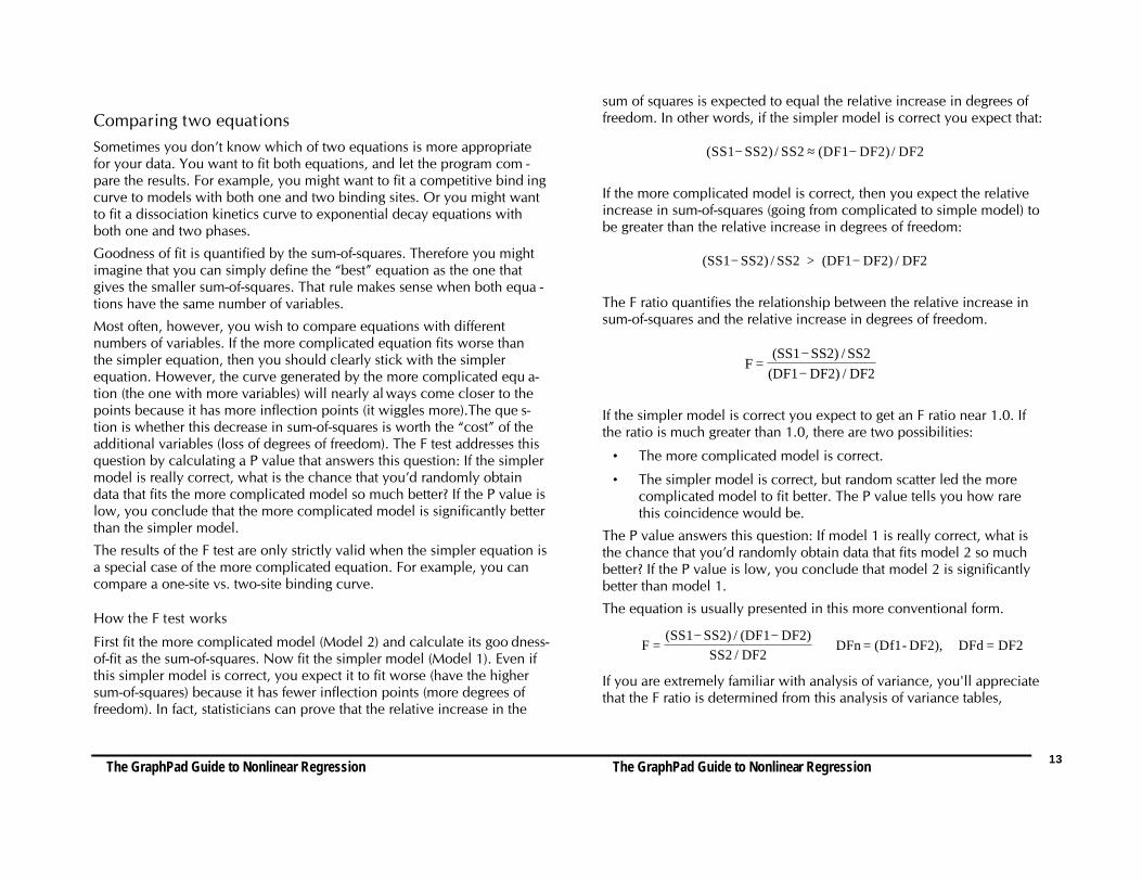
What to do when the fit is no good?The last section explained that a fit is bad when the fit did not converge,the results make no sense, or the confidence intervals are wide. If youencounter any of these situations, here are some things to try.

Potential problem SolutionThe equation simply does notdescribe the data.

Try a different equation.

The initial values are too far fromtheir correct values.

Enter different initial values. If you areusing a user-defined equation, check therules for initial values.

The range of X values is too na r-row to define the curve com-pletely.

If possible, collect more data. Other wise,hold one of the variables to a constantvalue.

You have not collected enoughdata in a critical range of X va l-ues.

Collect more data in the important re -gions.

Your data are very scattered anddon't really define a curve.

Try to collect less scattered data. If youare combining several experiments,normalize the data for each experimentto an internal control.

The equation includes more thanone component, but your datadon't follow a multicomponentmodel.

Use a simpler equation.

Your numbers are too large. If your Y values are huge, change theunits. Don't use values greater thanabout 104.

Your numbers are too small. If your Y values are tiny, change theunits. Don’t use values less than about10-4.


Comparing two equationsSometimes you don’t know which of two equations is more appropriatefor your data. You want to fit both equations, and let the program com -pare the results. For example, you might want to fit a competitive bind ingcurve to models with both one and two binding sites. Or you might wantto fit a dissociation kinetics curve to exponential decay equations withboth one and two phases.

Goodness of fit is quantified by the sum-of-squares. Therefore you mightimagine that you can simply define the “best” equation as the one thatgives the smaller sum-of-squares. That rule makes sense when both equa -tions have the same number of variables.

Most often, however, you wish to compare equations with differentnumbers of variables. If the more complicated equation fits worse thanthe simpler equation, then you should clearly stick with the simplerequation. However, the curve generated by the more complicated equ a-tion (the one with more variables) will nearly al ways come closer to thepoints because it has more inflection points (it wiggles more).The que s-tion is whether this decrease in sum-of-squares is worth the “cost” of theadditional variables (loss of degrees of freedom). The F test addresses thisquestion by calculating a P value that answers this question: If the simplermodel is really correct, what is the chance that you’d randomly obtaindata that fits the more complicated model so much better? If the P value islow, you conclude that the more complicated model is significantly betterthan the simpler model.

The results of the F test are only strictly valid when the simpler equation isa special case of the more complicated equation. For example, you cancompare a one-site vs. two-site binding curve.

How the F test works

First fit the more complicated model (Model 2) and calculate its goo dness-of-fit as the sum-of-squares. Now fit the simpler model (Model 1). Even ifthis simpler model is correct, you expect it to fit worse (have the highersum-of-squares) because it has fewer inflection points (more degrees offreedom). In fact, statisticians can prove that the relative increase in the

sum of squares is expected to equal the relative increase in degrees offreedom. In other words, if the simpler model is correct you expect that:

(SS1 SS2) / SS2 (DF1 DF2)/ DF2 − ≈ −

If the more complicated model is correct, then you expect the relativeincrease in sum-of-squares (going from complicated to simple model) tobe greater than the relative increase in degrees of freedom:

(SS1 SS2) / SS2 (DF1 DF2) / DF2 − > −

The F ratio quantifies the relationship between the relative increase insum-of-squares and the relative increase in degrees of freedom.

F(SS1 SS2) / SS2

(DF1 DF2) / DF2 =

−−

If the simpler model is correct you expect to get an F ratio near 1.0. Ifthe ratio is much greater than 1.0, there are two possibilities:

• The more complicated model is correct.

• The simpler model is correct, but random scatter led the morecomplicated model to fit better. The P value tells you how rarethis coincidence would be.

The P value answers this question: If model 1 is really correct, what isthe chance that you’d randomly obtain data that fits model 2 so muchbetter? If the P value is low, you conclude that model 2 is significantlybetter than model 1.

The equation is usually presented in this more conventional form.

F(SS1 SS2) / (DF1 DF2)

SS2 / DF2 DFn = (Df1- DF2), DFd = DF2=

− −

If you are extremely familiar with analysis of variance, you'll appreciatethat the F ratio is determined from this analysis of variance tables,


Source of variation Sum-of-squares df MSDifference SS1 - SS2 DF1 - DF2 SS1 - SS2

DF1 - DF2

Model 2 (complicated) SS2 DF2 SS2/DF2

Model 1 (simple) SS1 DF1

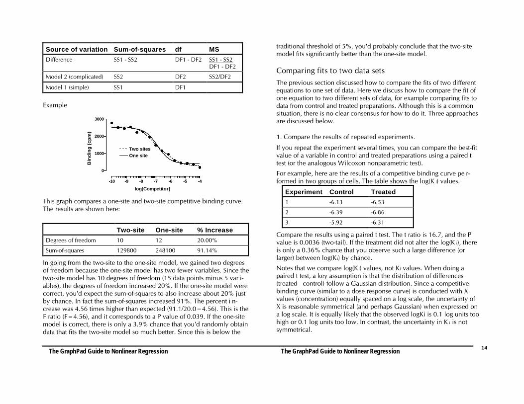
Example

log[Competitor]

Bin

din

g (

cpm

)

-10 -9 -8 -7 -6 -5 -4

0

1000

2000

3000

Two sitesOne site

This graph compares a one-site and two-site competitive binding curve.The results are shown here:

Two-site One-site % IncreaseDegrees of freedom 10 12 20.00%

Sum-of-squares 129800 248100 91.14%

In going from the two-site to the one-site model, we gained two degreesof freedom because the one-site model has two fewer variables. Since thetwo-site model has 10 degrees of freedom (15 data points minus 5 var i-ables), the degrees of freedom increased 20%. If the one-site model werecorrect, you'd expect the sum-of-squares to also increase about 20% justby chance. In fact the sum-of-squares increased 91%. The percent i n-crease was 4.56 times higher than expected (91.1/20.0=4.56). This is theF ratio (F=4.56), and it corresponds to a P value of 0.039. If the one-sitemodel is correct, there is only a 3.9% chance that you'd randomly obtaindata that fits the two-site model so much better. Since this is below the

traditional threshold of 5%, you'd probably conclude that the two-sitemodel fits significantly better than the one-site model.

Comparing fits to two data setsThe previous section discussed how to compare the fits of two differentequations to one set of data. Here we discuss how to compare the fit ofone equation to two different sets of data, for example comparing fits todata from control and treated preparations. Although this is a commonsituation, there is no clear consensus for how to do it. Three approachesare discussed below.

1. Compare the results of repeated experiments.

If you repeat the experiment several times, you can compare the best-fitvalue of a variable in control and treated preparations using a paired ttest (or the analogous Wilcoxon nonparametric test).

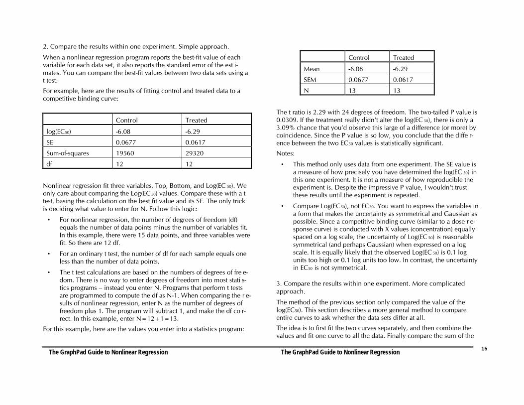
For example, here are the results of a competitive binding curve pe r-formed in two groups of cells. The table shows the log(K i) values.

Experiment Control Treated1 -6.13 -6.53

2 -6.39 -6.86

3 -5.92 -6.31

Compare the results using a paired t test. The t ratio is 16.7, and the Pvalue is 0.0036 (two-tail). If the treatment did not alter the log(K i), thereis only a 0.36% chance that you observe such a large difference (orlarger) between log(K i) by chance.

Notes that we compare log(K i) values, not Ki values. When doing apaired t test, a key assumption is that the distribution of differences(treated - control) follow a Gaussian distribution. Since a competitivebinding curve (similar to a dose response curve) is conducted with Xvalues (concentration) equally spaced on a log scale, the uncertainty ofX is reasonable symmetrical (and perhaps Gaussian) when expressed ona log scale. It is equally likely that the observed logKi is 0.1 log units toohigh or 0.1 log units too low. In contrast, the uncertainty in K i is notsymmetrical.


2. Compare the results within one experiment. Simple approach.

When a nonlinear regression program reports the best-fit value of eachvariable for each data set, it also reports the standard error of the est i-mates. You can compare the best-fit values between two data sets using at test.

For example, here are the results of fitting control and treated data to acompetitive binding curve:

Control Treated

log(EC50) -6.08 -6.29

SE 0.0677 0.0617

Sum-of-squares 19560 29320

df 12 12

Nonlinear regression fit three variables, Top, Bottom, and Log(EC 50). Weonly care about comparing the Log(EC 50) values. Compare these with a ttest, basing the calculation on the best fit value and its SE. The only trickis deciding what value to enter for N. Follow this logic:

• For nonlinear regression, the number of degrees of freedom (df)equals the number of data points minus the number of variables fit.In this example, there were 15 data points, and three variables werefit. So there are 12 df.

• For an ordinary t test, the number of df for each sample equals oneless than the number of data points.

• The t test calculations are based on the numbers of degrees of fre e-dom. There is no way to enter degrees of freedom into most stati s-tics programs – instead you enter N. Programs that perform t testsare programmed to compute the df as N-1. When comparing the r e-sults of nonlinear regression, enter N as the number of degrees offreedom plus 1. The program will subtract 1, and make the df co r-rect. In this example, enter N=12+1=13.

For this example, here are the values you enter into a statistics program:

Control Treated

Mean -6.08 -6.29

SEM 0.0677 0.0617

N 13 13

The t ratio is 2.29 with 24 degrees of freedom. The two-tailed P value is0.0309. If the treatment really didn't alter the log(EC 50), there is only a3.09% chance that you'd observe this large of a difference (or more) bycoincidence. Since the P value is so low, you conclude that the diffe r-ence between the two EC50 values is statistically significant.

Notes:

• This method only uses data from one experiment. The SE value isa measure of how precisely you have determined the log(EC 50) inthis one experiment. It is not a measure of how reproducible theexperiment is. Despite the impressive P value, I wouldn't trustthese results until the experiment is repeated.

• Compare Log(EC50), not EC50. You want to express the variables ina form that makes the uncertainty as symmetrical and Gaussian aspossible. Since a competitive binding curve (similar to a dose r e-sponse curve) is conducted with X values (concentration) equallyspaced on a log scale, the uncertainty of Log(EC 50) is reasonablesymmetrical (and perhaps Gaussian) when expressed on a logscale. It is equally likely that the observed Log(EC 50) is 0.1 logunits too high or 0.1 log units too low. In contrast, the uncertaintyin EC50 is not symmetrical.

3. Compare the results within one experiment. More complicatedapproach.

The method of the previous section only compared the value of thelog(EC50). This section describes a more general method to compareentire curves to ask whether the data sets differ at all.

The idea is to first fit the two curves separately, and then combine thevalues and fit one curve to all the data. Finally compare the sum of the


two individual sum-of-squares values with the sum-of-squares from thecombined data.

Follow these steps:

1. Fit the two data sets separately. We did this in the previous se ction.

2. Total the sum-of-squares and df from the two fits. For this examplethe total sum of squares equals. 19560+29320= 48880, and the t o-tal df equals 12+12=24. Since these are the results of fitting thetwo data sets separately, label these values SS separate and DFseparate

3. Combine the two data sets into one. For this example, the co m-bined data set has XY pairs, with each X value appearing in twice.

4. Fit the combined data set to the same equation. Note the SS and df.For this example, SS=165200, and df=27 (30 data points minusthree variables). Call these values SScombined and Dfcombined.

5. You expect SSseparate to be smaller than SS combined even if thecurves are really identical simply because the separate fits havemore degrees of freedom. The question is whether the SS values aremore different than you'd expect to see by chance. To find out, ca l-culate the F ratio using this equation:

( ) ( )F

SS SS / DF DF

SS / DFcombined separate combined separate

combined separate

=− −

For this example, F = 19.03.

6. Determine the P value from F. There are DF combined - DFseparatedegrees of freedom in the numerator, and DF separate degrees offreedom in the denominator. If you don't have a program that doesthis, consult tables in the back of most statistics books.

7. For this example, the P value is less than 0.0001. If the treatmentwere really ineffective, there is less than a 0.01% chance that thetwo curves would differ as much (or more) than observed in thisexperiment. Since the P value is low, you'll conclude that thecurves are really different.

Notes:

• This method only uses data from one experiment. I wouldn't trustthese results until the experiment is repeated.

• This method compares the curves overall. It doesn't tell you whichvariable(s) are different. Differences might be due to somethingtrivial like a different baseline, rather than something importantlike a different rate constant.

Advantages and disadvantages of the three methods

If you have repeated the experiment several times, I recommend thatyou use the first method. There are two advantages:

• Compared to the other methods discussed below, this method isfar easier to understand and communicate to others.

• The entire test is based on the consistency of the results betweenrepeat experiments. Since there are usually more causes for var i-ability between experiments than within experiments, it makessense to base the comparison on differences between exper i-ments.

The disadvantage of the first method is that you are throwing awayinformation. The calculations are based only on the best-fit value fromeach experiment, and ignores the SE of those values presented by thecurve fitting program.

If you have performed the experiment only once, then you probablyought to repeat the experiment. Regardless of what statistical results youobtain, you shouldn't trust results from a single experiment. If you wantto compare results in a single experiment, you can use method 2 ormethod 3.

The advantage of method 2 is that it focuses your thinking on a singlevariable. Generally, you care mostly about one variable (i.e. a rateconstant or EC50), and care less about the others. Method 2 comparesthe variable of interest.

Method 3 is the most general method. Since the method compares theentire curve, it does not force you to decide which variable(s) you wishto compare. This is both its advantage and disadvantage.


GraphPad Prism

All the graphs in this booklet were created using GraphPad Prism, ageneral-purpose curve fitting and scientific graphics program for Wi n-dows.

Although GraphPad Prism was designed to be a general purpose program,it is particularly well-suited for nonlinear regression:

• Prism provides a menu of commonly-used equations (includingequations used for analysis of radioligand binding experiments). Tofit a curve, all you have to do is pick the right equation. Prism doesall the rest automatically, from picking initial values to graphing thecurve.

• Prism can automatically compare two models with the F test.

• When analyzing competitive radioligand binding curves, Prismautomatically calculates K i from IC50.

• You can use the best-fit curve as a standard curve. Enter Y valuesand Prism will determine X. Or enter X and Prism will determine Y.

• Prism can automatically graph a residual plot and perform the runstest.

• Prism’s manual and help screens explain the principles of curvefitting with nonlinear regression and help you interpret the results.You don’t have to be a statistics expert to use Prism.

Please visit our web site at http://www.graphpad.com. You can readabout the Prism and download a free demo. Or contact GraphPad Sof t-ware to request a brochure and demo disk by phone (619-457-3909), fax(619-457-8141) or email ([email protected]) . The demo is not a slideshow – it is a functional version of Prism with no limitations in dataanalysis. Try it out with your own data, and see for yourself why Prism isthe best solution for analyzing and graphing scientific data.

Documents

GraphPad Guide to Nonlinear Regression - IBCCFfisbio.biof.ufrj.br/.../bioEstatistica/90_top_especiais/nonlin.pdf · The GraphPad Guide to Nonlinear Regression The GraphPad Guide to