Embed Size (px)
Citation preview
Gravitino Dark Matter and
Light elements abundance
Vassilis SpanosDept of Physics, University of Patras
Cyburt, Ellis, Fields, Olive
Outline
Cosmological data and Big-Bang Nucleosynthesis (BBN) constraints
Gravitino DM scenarios
New phenomena (stau bound states effects)
Summary-Prospects
The SN Ia data suggested that
ΩΛ = 43
ΩM + 13± 1
6.
FromCMB anisotropy the total matter-energy density is Ω0 = 1.0±0.1
From various measurements ΩM = 0.35±0.1 . Hence the cosmologicalconstant contribution is
ΩΛ = 0.8 ± 0.2
The baryonic density is ΩB = 0.045 ± 0.001 , subtracted from the total
matter density gives the Dark Matter density
ΩDM ! 0.3 ± 0.1
The Hubble parameter is estimated with fairly good accuracy
h0 = 0.65 ± 0.05 =⇒
ΩDM h02 ! 0.13 ± 0.05
V.C. Spanos, Univ. of Minnesota VCMSSM 26This value of agrees with the BBN predictions
Ωtot = 1.0 ± 0.1
ΩM = 0.3 ± 0.04
ΩB = 0.05 ± 0.004
ΩDM = Ωm − ΩB ∼ 0.25 ± 0.04
[J. Ellis, J.S. Hagelin, D.V. Nanopoulos, K.A. Olive and M. Srednicki, NPB238 (1984)
453]
V.C. Spanos, Univ. of Minnesota VCMSSM 26
No Big Bang
1 20 1 2 3
expands forever
!1
0
1
2
3
2
3
closed
Supernovae
CMB
Clusters
SNe: Knop et al. (2003)CMB: Spergel et al. (2003)Clusters: Allen et al. (2002)
"#
"M
open
flat
recollapses eventually
and
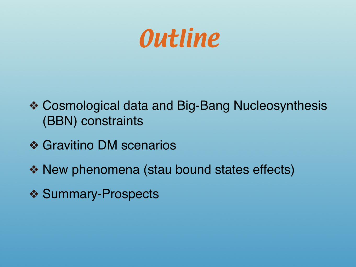
with all of them?
Ωtot = 1.02 ± 0.02
Ωm = 0.25 ± 0.01
ΩB = 0.043 ± 0.002
ΩDM = Ωm − ΩB ∼ 0.21 ± 0.01
[J. Ellis, J.S. Hagelin, D.V. Nanopoulos, K.A. Olive and M. Srednicki, NPB238 (1984)
453]
V.C. Spanos, Univ. of Minnesota VCMSSM 26
Ωtot = 1.02 ± 0.02
Ωm h20 = 0.134 ± 0.006
ΩB h20 = 0.023 ± 0.001
ΩDM h20 = Ωm h2
0 − ΩB h20 = 0.25 ∼ 0.111 ± 0.006
[J. Ellis, J.S. Hagelin, D.V. Nanopoulos, K.A. Olive and M. Srednicki, NPB238 (1984)
453]
V.C. Spanos, Univ. of Minnesota VCMSSM 26
Ωtot = 1.02 ± 0.02
Ωm h20 = 0.134 ± 0.006
ΩB h20 = 0.023 ± 0.001
ΩDM h20 = Ωm h2
0 − ΩB h20 = 0.25 ∼ 0.111 ± 0.006
[J. Ellis, J.S. Hagelin, D.V. Nanopoulos, K.A. Olive and M. Srednicki, NPB238 (1984)
453]
V.C. Spanos, Univ. of Minnesota VCMSSM 26
Ωtot = 1.02 ± 0.02
Ωm h20 = 0.134 ± 0.006
ΩB h20 = 0.023 ± 0.001
ΩDM h20 = Ωm h2
0 − ΩB h20 = 0.111 ± 0.006
[J. Ellis, J.S. Hagelin, D.V. Nanopoulos, K.A. Olive and M. Srednicki, NPB238 (1984)
453]
V.C. Spanos, Univ. of Minnesota VCMSSM 26
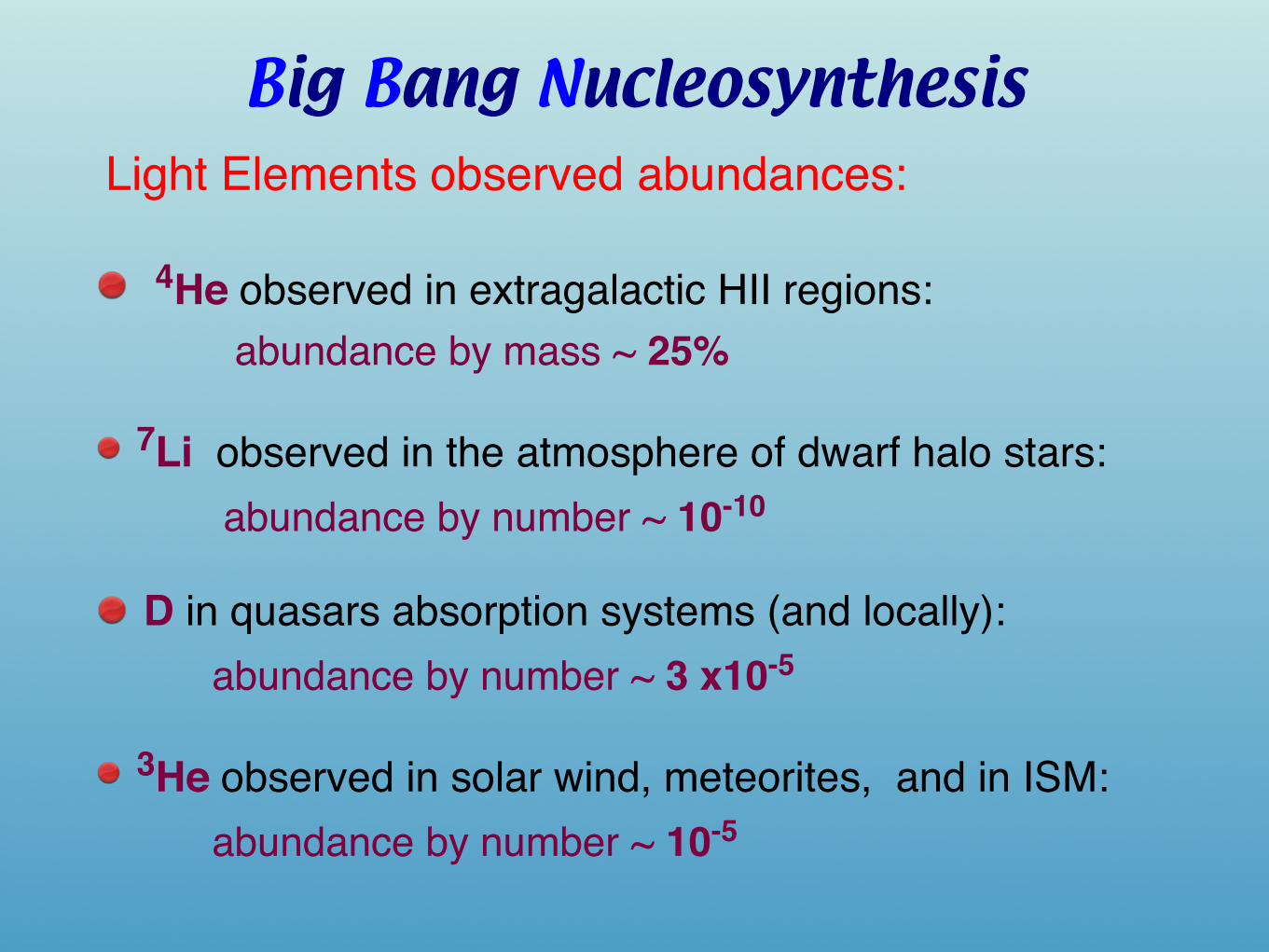
4He observed in extragalactic HII regions: abundance by mass ~ 25%
7Li observed in the atmosphere of dwarf halo stars: abundance by number ~ 10-10
D in quasars absorption systems (and locally): abundance by number ~ 3 x10⁻⁵
3He observed in solar wind, meteorites, and in ISM: abundance by number ~ 10-5
Big Bang Nucleosynthesis Light Elements observed abundances:
Production of light elements: D, 3He, 4He, 7Li, 6Li
D 3He 4He 7Li 6Li
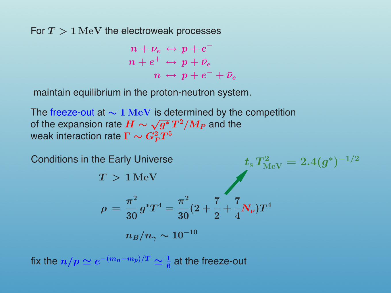
For T > 1 MeV the electroweak processes
n + νe ↔ p + e−
n + e+ ↔ p + νe
n ↔ p + e− + νe
maintain equilibrium in the proton-neutron system.
The freeze-out at ∼ 1 MeV is determined by the competition
of the expansion rate H ∼√
g∗ T 2/MP and the
weak interaction rate Γ ∼ G2FT 5
Initial conditions:
T > 1 MeV
ρ =π2
30g∗T 4 =
π2
30(2 +
7
2+
7
4Nν)T
4
nB/nγ ∼ 10−10
V.C. Spanos, Univ. of Minnesota VCMSSM 35
Conditions in the Early Universe
T > 1 MeV
ρ =π2
30g∗T 4 =
π2
30(2 +
7
2+
7
4Nν)T
4
nB/nγ ∼ 10−10
fix the n/p $ 16at the freeze-out
ts T 2MeV = 2.4(g∗)−1/2
V.C. Spanos, Univ. of Minnesota VCMSSM 36
Conditions in the Early Universe
T > 1 MeV
ρ =π2
30g∗T 4 =
π2
30(2 +
7
2+
7
4Nν)T
4
nB/nγ ∼ 10−10
fix the n/p $ e−(mn−mp)/T $ 16at the freeze-out
ts T 2MeV = 2.4(g∗)−1/2
V.C. Spanos, Univ. of Minnesota VCMSSM 36
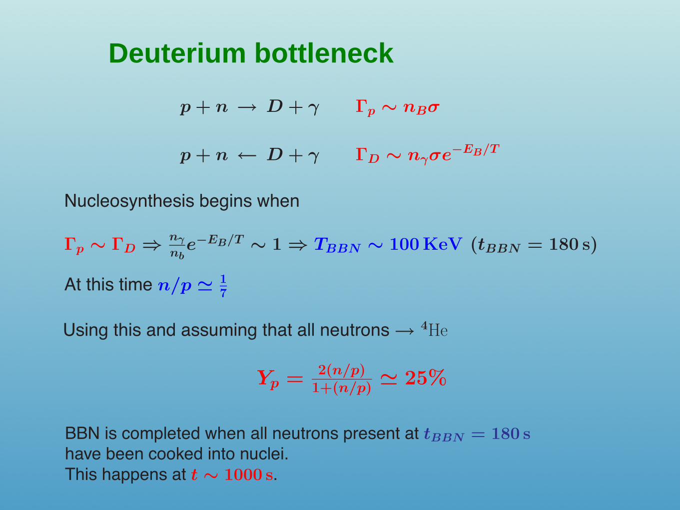
Deuterium bottleneck
Using this and assuming that all neutrons → 4He
Yp = 2(n/p)1+(n/p)
" 25%
BBN is completed when all neutrons present at tBBN = 180shave been cooked into nuclei. This happens at t ∼ 1000 s 3 min
V.C. Spanos, Univ. of Minnesota VCMSSM 38
Using this and assuming that all neutrons → 4He
Yp = 2(n/p)1+(n/p)
" 25%
BBN is completed when all neutrons present at tBBN = 180shave been cooked into nuclei. This happens at t ∼ 1000 s 3 min
V.C. Spanos, Univ. of Minnesota VCMSSM 38
Using this and assuming that all neutrons → 4He
Yp = 2(n/p)1+(n/p)
" 25%
BBN is completed when all neutrons present at tBBN = 180 shave been cooked into nuclei.
This happens at t ∼ 1000 s.
V.C. Spanos, Univ. of Minnesota VCMSSM 38
p + n → D + γ Γp ∼ nBσ
p + n ← D + γ ΓD ∼ nγσe−EB/T
Nucleosynthesis begins when
Γp ∼ ΓD ⇒ nγ
nbe−EB/T ∼ 1 ⇒ TBBN ∼ 100KeV (tBBN = 180 s)
At this time n/p & 17
V.C. Spanos, Univ. of Minnesota VCMSSM 37
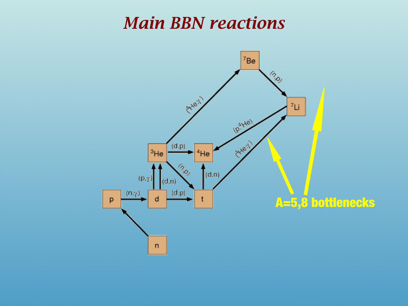
Main BBN reactions
A=5,8 bottlenecks
141
10-25
10-20
10-15
10-10
10-5
1 0.1 0.01
p
n
2H
4He
3H
3He
7Li
7Be
6Li
T (MeV)
A /
H
!
"
n
N
= 887 sec
N = 3
= 0.01h#
-2
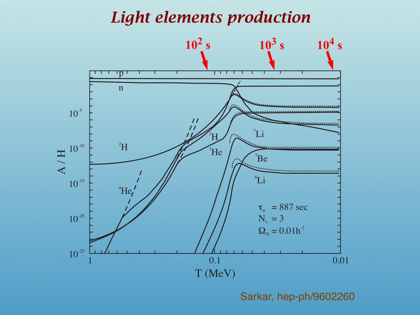
Figure 3. Evolution of the abundances of primordially synthesized light elements with
temperature according to the Wagoner (1973) numerical code as upgraded by Kawano
(1992). The dashed lines show the values in nuclear statistical equilibrium while the
dotted lines are the ‘freeze-out’ values as calculated analytically by Esmailzadeh et al
(1991).
Light elements production
Sarkar, hep-ph/9602260
103 s 104 s102 s
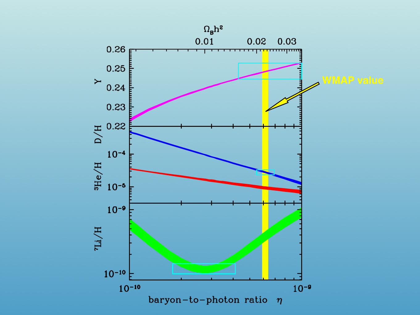
WMAP value
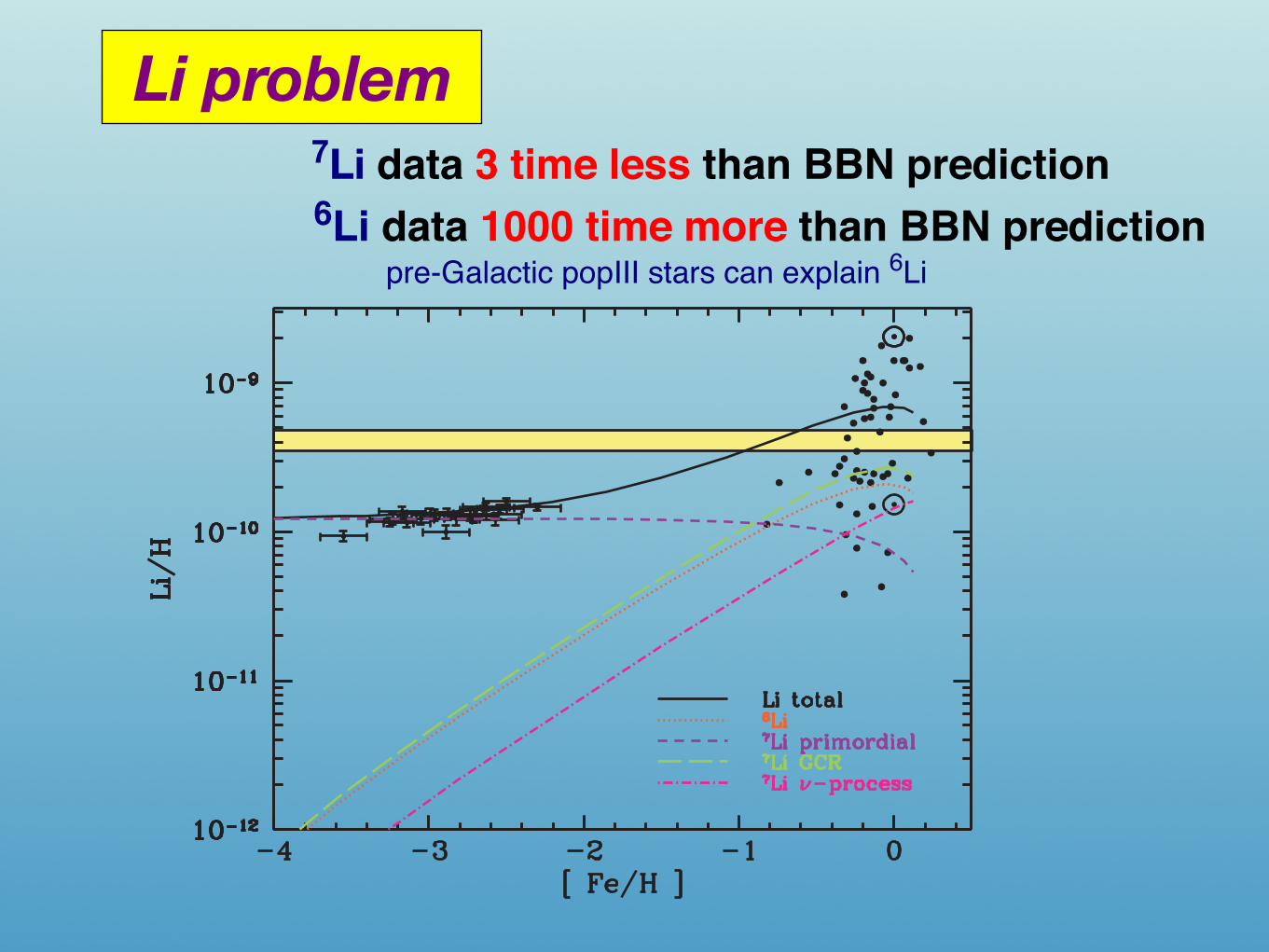
Li problem 7Li data 3 time less than BBN prediction 6Li data 1000 time more than BBN prediction
pre-Galactic popIII stars can explain 6Li
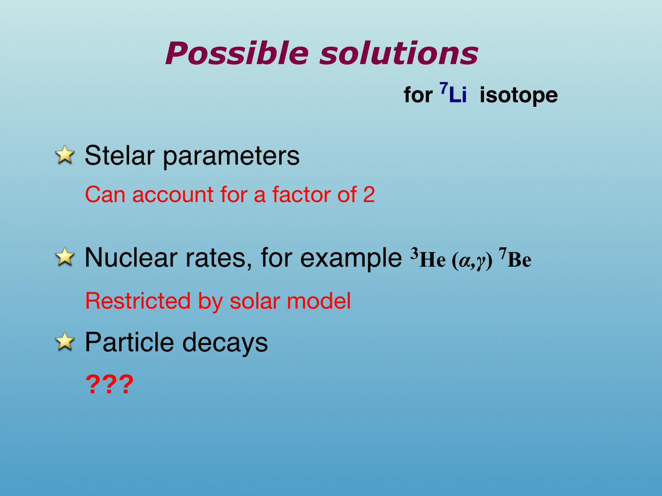
Stelar parametersCan account for a factor of 2
Nuclear rates, for example 3He (α,γ) 7Be
Restricted by solar model Particle decays ???
Possible solutionsfor 7Li isotope
• Sneutrino (constrained severely by LEP2 data and direct data)
• Neutralino
• Gravitino
SUSY Candidates for Dark Matter
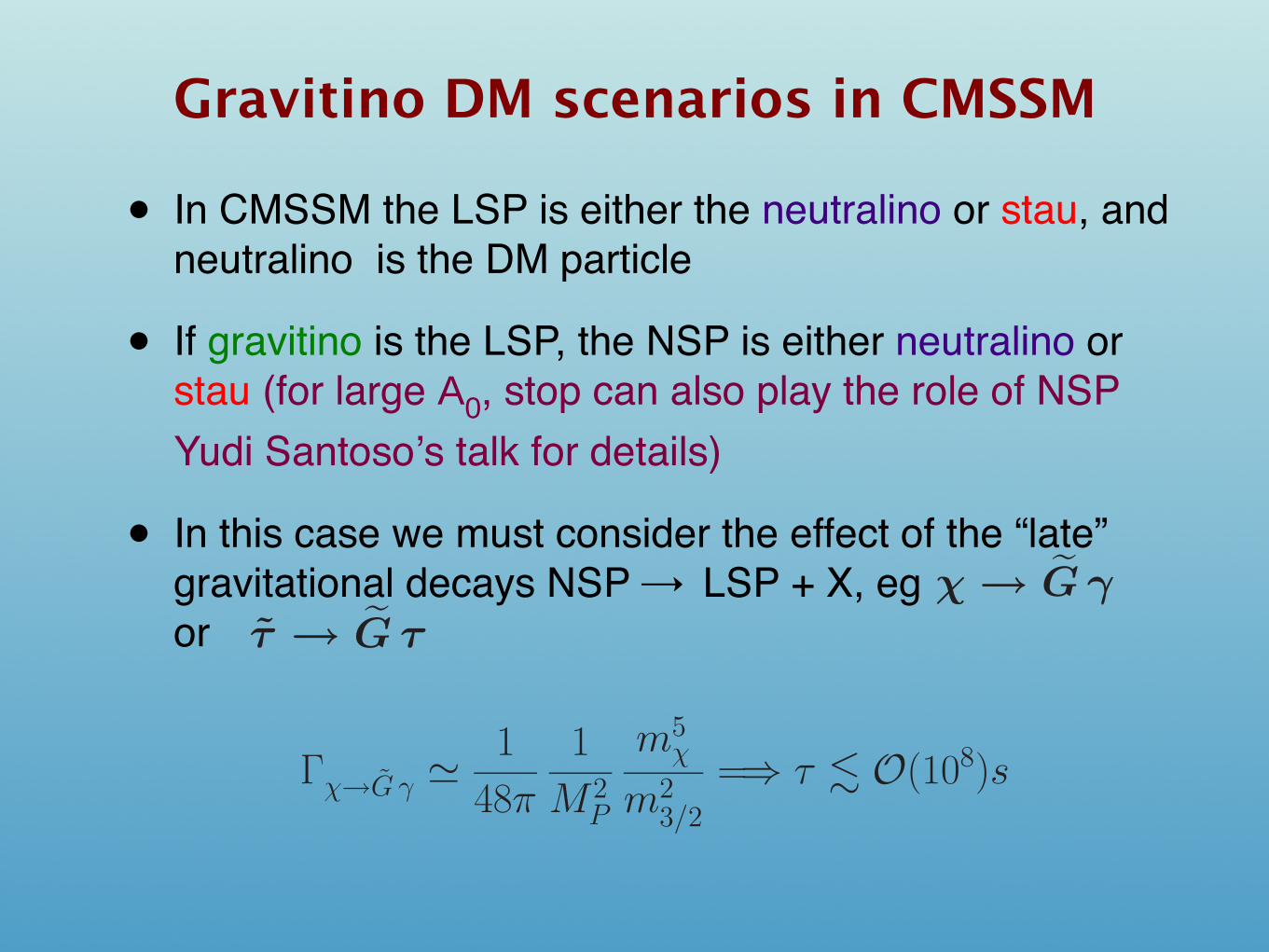
• In CMSSM the LSP is either the neutralino or stau, and neutralino is the DM particle
• If gravitino is the LSP, the NSP is either neutralino or stau (for large A0, stop can also play the role of NSP Yudi Santoso’s talk for details)
• In this case we must consider the effect of the “late” gravitational decays NSP → LSP + X, eg or
Gravitino DM scenarios in CMSSM
χ → G γ
χ → G Z
χ → G Hi
τ → G τ
3He(α, γ)7Be
V.C. Spanos, Univ. of Minnesota VCMSSM 39
χ → G γ
χ → G Z
χ → G Hi
τ → G τ
3He(α, γ)7Be
V.C. Spanos, Univ. of Minnesota VCMSSM 39
The dominant decay of a χ NSP would be into a gravitino and a pho-ton, for which we calculate the width
Γχ→G γ =1
16π
C2χγ
M 2P
m5χ
m23/2
(
1 −m2
3/2
m2χ
)3 (1
3+
m23/2
m2χ
)
where Cχγ = (O1χ cos θW + O2χ sin θW ) and O is the neutralino diagonal-
ization matrix, OT MN O = MdiagN
MP ≡ 1/√
8πGN
Γχ→G γ %1
48π
1
M 2P
m5χ
m23/2
=⇒ τ ! O(108)s
V.C. Spanos, Univ. of Minnesota VCMSSM 15
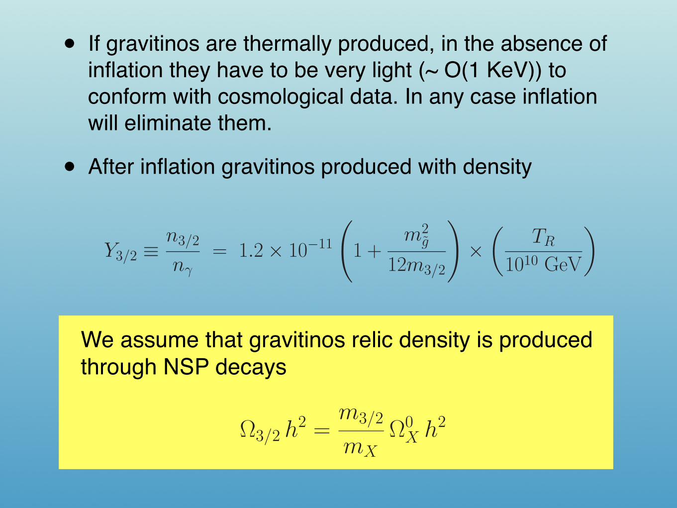
• If gravitinos are thermally produced, in the absence of inflation they have to be very light (~ O(1 KeV)) to conform with cosmological data. In any case inflation will eliminate them.
• After inflation gravitinos produced with density
! The prospect that gravitino is the DM candidate, has been studied
extensively in the past.
! If the gravitinos are thermally produced, in the absence of inflation,
they have to be very light, to conform with the cosmological data
! O(1) KeV. But inflation will eliminate any gravitino relic density.
! Gravitino can be thermally produced after inflation, with relic density
Y3/2 ≡n3/2
nγ= 1.2 × 10⁻¹¹
(
1 +m2
g
12m3/2
)
×(
TR
1010 GeV
)
where TR is the reheating temperature at the end of the inflationary
epoch.
V.C. Spanos, Univ. of Minnesota VCMSSM 5
We assume that gravitinos relic density is produced through NSP decays
! We assume that the gravitinos’ relic density is produced from the
decays of NSP:X = χ or τ . On this basis we estimated the gravitinoDM density as
Ω3/2 h2 =m3/2
mXΩ0
X h2
V.C. Spanos, Univ. of Minnesota VCMSSM 12
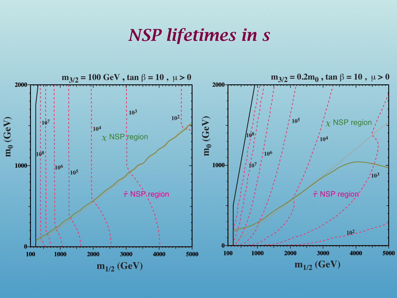
NSP lifetimes in s
τ NSP region
χ NSP region
V.C. Spanos, Univ. of Minnesota VCMSSM 41
τ NSP region
χ NSP region
V.C. Spanos, Univ. of Minnesota VCMSSM 41
τ NSP region
χ NSP region
V.C. Spanos, Univ. of Minnesota VCMSSM 41
τ NSP region
χ NSP region
V.C. Spanos, Univ. of Minnesota VCMSSM 41
100 1000 2000 3000 4000 5000
0
1000
2000
100 1000 2000 3000 4000 5000
0
1000
2000
m0 (
GeV
)
m1/2 (GeV)
m3/2 = 100 GeV , tan ! = 10 , ! > 0
108
107
106
105
104
103
102
100 1000 2000 3000 4000 5000
0
1000
2000
100 1000 2000 3000 4000 5000
0
1000
2000
m0 (
GeV
)
m1/2 (GeV)
m3/2 = 0.2m0 , tan ! = 10 , ! > 0
105
102
103
104
106
107
108
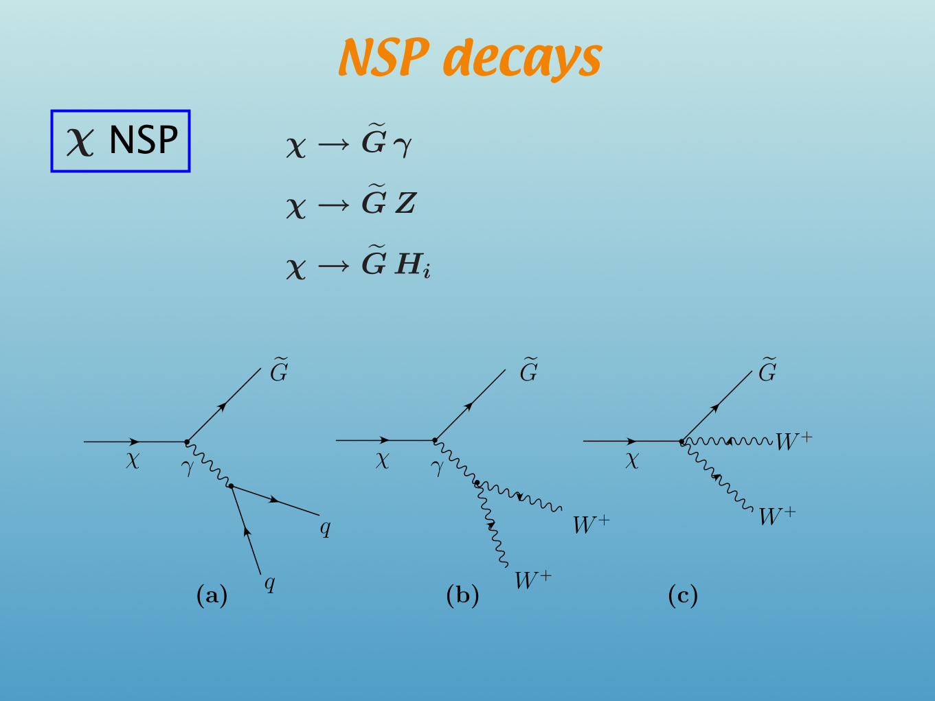
NSP decaysNSP χ → G γ
χ → G Z
χ → G Hi
V.C. Spanos, Univ. of Minnesota VCMSSM 39
χ γ
G
q
q
(a)
χ γ
G
W+
W+
(b)
χ
G
W+
W+
(c)
Figure 1: Hadronic 3-body decays for the gravitino LSP and χ NSP case.
boson, the next most important channel is χ → G Z, which is also the dominant channel for
producing HD injections in this case. The Higgs boson channels are smaller by a few orders
of magnitude, and those to heavy Higgs bosons (H, A) in particular become kinematically
accessible only for heavy χ in the large-m1/2 region. Turning to the three-body channels, the
decay through the virtual photon to a qq pair can become comparable to the subdominant
channel χ → G Z, injecting nucleons even in the kinematical region mχ < m3/2 +MZ , where
direct on-shell Z-boson production is not possible 1. Finally, we note that the three-body
decays to W+W− pairs and a gravitino are usually at least five orders of magnitude smaller.
Having calculated the partial decay widths and branching ratios, we employ the PYTHIA
event generator [28] to model both the EM and the HD decays of the direct products of the
χ decays. We first generate a sufficient number of spectra for the secondary decays of the
gauge and Higgs bosons and the quark pairs. Then, we perform fits to obtain the relation
between the energy of the decaying particle and the quantity that characterizes the hadronic
spectrum, namely dNh/dEh, the number of produced nucleons as a function of the nucleon
energy. These spectra and the fraction of the energy of the decaying particle that is injected
as EM energy are then used to calculate the light-element abundances.
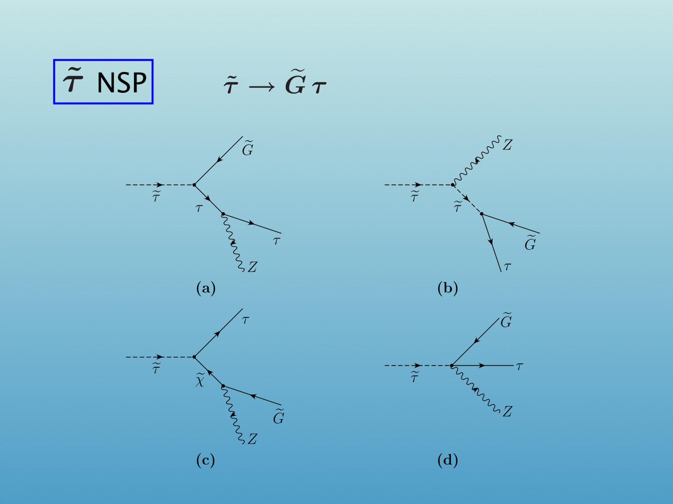
An analogous procedure is followed for the τ NSP case. As the lighter stau is predomi-
nantly right-handed, its interactions with W bosons are very weak (suppressed by powers of
mτ ) and can be ignored. The decay rate for the dominant two-body decay channel, namely
τ → G τ , has been given in [19]. However, this decay channel does not yield any nucle-
ons. Therefore, one must calculate some three-body decays of the τ to obtain any protons
or neutrons. The most relevant channels are τ → G τ ∗ → G Z τ , τ → Z τ ∗ → G Z τ ,
1In principle, one should also include qq pair production through the virtual Z-boson channel χ → G Z∗ →G qq [6] and the corresponding interference term. However, this process is suppressed by a factor of M4
Z
with respect to χ → G γ∗ → G qq, and the interference term is also suppressed by M2Z. Numerically, these
contributions are unimportant, and therefore we drop these amplitudes in our calculation.
9
χ → G γ
χ → G Z
χ → G Hi
τ → G τ
3He(α, γ)7Be
V.C. Spanos, Univ. of Minnesota VCMSSM 39
NSP
χ → G γ
χ → G Z
χ → G Hi
τ → G τ
V.C. Spanos, Univ. of Minnesota VCMSSM 39
ττ
G
Z
τ
(a)
τ
G
τ
Z
τ
(b)
τχ
τ
Z
G
(c)
τ
G
τ
Z
(d)
Figure 2: Hadronic 3-body decays for the τ NSP case.
τ → τχ∗ → G Z τ and τ → G Z τ [18] and they are presented in Fig. 2. We calculate these
partial widths, and then use PYTHIA to obtain the hadronic spectra and the EM energy
injected by the secondary Z-boson and τ -lepton decays. As in the case of the χ NSP, this
information is then used for the BBN calculation.
We stress that this procedure is repeated separately for each point in the supersymmetric
parameter space sampled. That is, given a set of parameters m0, m1/2, A0, tanβ, sgn(µ), and
m3/2, once the sparticle spectrum is determined, all of the relevant branching fractions are
computed, and the hadronic spectra and the injected EM energy determined case by case.
For this reason, we do not use a global parameter such as the hadronic branching fraction,
Bh, often used in the literature. In our analysis, Bh is computed and differs at each point in
the parameter space.
5 Results
5.1 Analytic Discussion
Outline basic qualitative effects: hadronic decays of X affect BBN in different ways depend-
ing on the stage of BBN in which the nonthermal decay particles interact with the background
thermal nuclei. This effectively divides the decay effects according to the decaying particle’s
lifetime τX .
10
χ → G γ
χ → G Z
χ → G Hi
τ → G τ
3He(α, γ)7Be
V.C. Spanos, Univ. of Minnesota VCMSSM 39
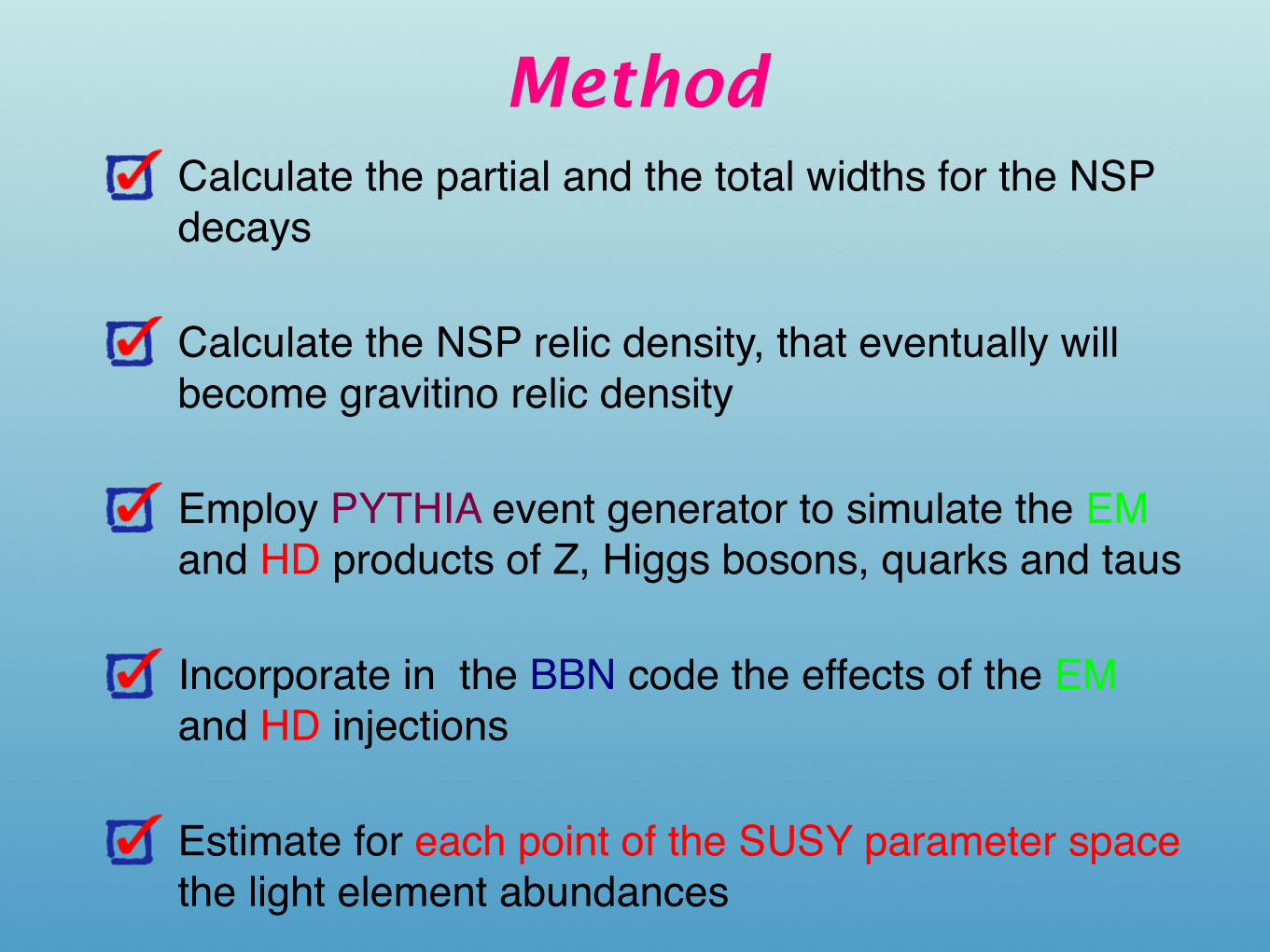
Method Calculate the partial and the total widths for the NSP decays
Calculate the NSP relic density, that eventually will become gravitino relic density
Employ PYTHIA event generator to simulate the EM and HD products of Z, Higgs bosons, quarks and taus
Incorporate in the BBN code the effects of the EM and HD injections
Estimate for each point of the SUSY parameter space the light element abundances
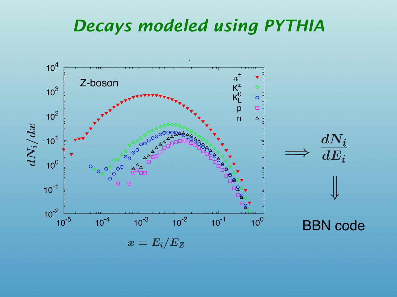
Decays modeled using PYTHIA
10-2
10-1
100
101
102
103
104
10-5
10-4
10-3
10-2
10-1
100
dN
i/dx
x=sqrt(Ei2-pi
2)/Einj
Z-boson HD spectra, Einj=1000 GeV
!!
K!
KL0
p
n
τNSPregion
χNSPregion
u,d,c,
s,t,
b
e,µ,τ,ν
e,ν
µ,ν
τ
γ,Z,W
±,g
u,d,c,
s,t,
b
e,µ,τ,ν
e,ν
µ,ν
τ
γ,Z,W
±,g
H1,2
⇐⇒
dN
i/dx
x=
Ei/
EZ
V.C
.Spa
nos,
Uni
v.of
Min
neso
taVCMSSM41
τ NSP region
χ NSP region
u, d, c, s, t, b
e, µ, τ , νe, νµ, ντ
γ, Z, W ±, g
u, d, c, s, t, b
e, µ, τ , νe, νµ, ντ
γ, Z, W ±, g
H1,2
⇐⇒
dNi/dx
x = Ei/EZ
V.C. Spanos, Univ. of Minnesota VCMSSM 41
τNSPregion
χNSPregion
u,d,c,s,t,
b
e,µ,τ,ν
e ,ν
µ,ν
τ
γ,Z,W
±,g
u,d,c,s,t,
b
e,µ,τ,ν
e ,ν
µ,ν
τ
γ,Z,W
±,g
H1,2
⇐⇒
=⇒
dN
i /dE
i
V.C.S
panos,Univ.
ofMinnesota
VCMSSM41
τ NSP region
χ NSP region
u, d, c, s, t, b
e, µ, τ , νe, νµ, ντ
γ, Z, W ±, g
u, d, c, s, t, b
e, µ, τ , νe, νµ, ντ
γ, Z, W ±, g
H1,2
⇐⇒
=⇒dNidEi
V.C. Spanos, Univ. of Minnesota VCMSSM 41
τ NSP region
χ NSP region
u, d, c, s, t, b
e, µ, τ , νe, νµ, ντ
γ, Z, W ±, g
u, d, c, s, t, b
e, µ, τ , νe, νµ, ντ
γ, Z, W ±, g
H1,2
⇐⇒
=⇒
dNi/dEi
V.C. Spanos, Univ. of Minnesota VCMSSM 41BBN code
Z-boson
Bound-state effects
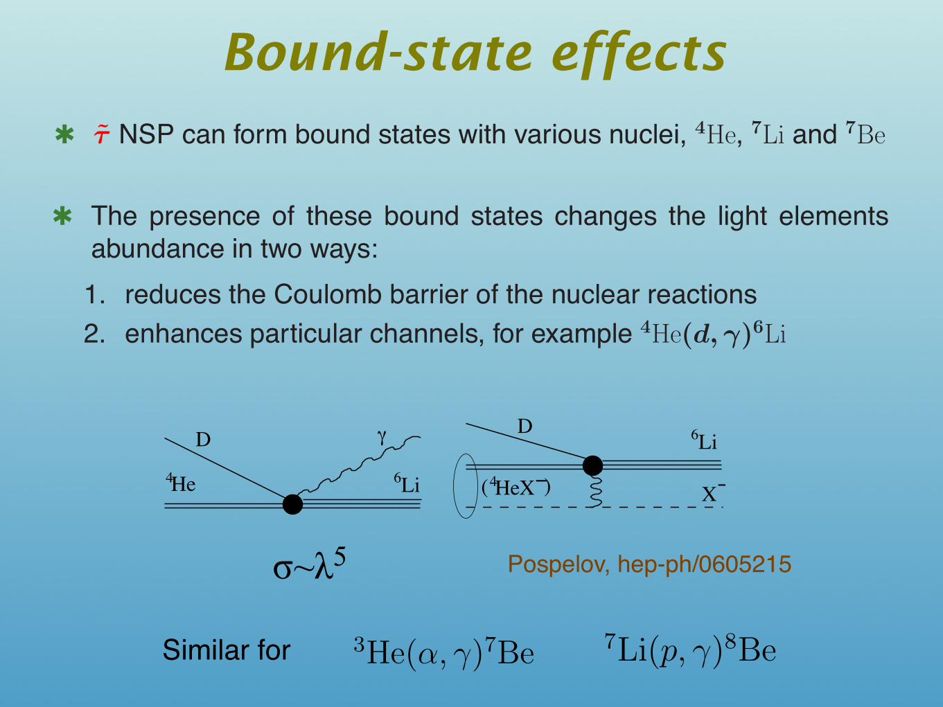
! τ NSP can form bound states with various nuclei, 4He, 7Li and 7Be
! The presence of these bound states changes the light elements
abundance in two ways:
1. reduces the Coulomb barrier of the nuclear reactions
2. enhances particular channels, for example 4He(d, γ)6Li
! We discussed alternatives to the Constrained scenario, the NUHM,
LEEST. In those cases the cosmologically favored regions increase.
! LHC will explore the bulk of the parameter space of CMSSM, al-
though some models, especially with large tan β are not covered.
! A LC with ECM = 1000 GeV clearly has a good chance of pro-ducing sparticles, but this still cannot be guaranteed. A LC with
ECM = 3000GeV seems ‘guaranteed’ to produce and detect spar-ticles, within CMSSM. HigherECM might be required in some GDM
scenarios.
V.C. Spanos, Univ. of Minnesota VCMSSM 40
2
bound st. |E0b | a0 Rsc
N |Eb(RscN )| RNc |Eb(RNc)| T0
4HeX− 397 3.63 1.94 352 2.16 346 8.26LiX− 1343 1.61 2.22 930 3.29 780 197LiX− 1566 1.38 2.33 990 3.09 870 217BeX− 2787 1.03 2.33 1540 3 1350 328BeX− 3178 0.91 2.44 1600 3 1430 34
4HeX−− 1589 1.81 1.94 1200 2.16 1150 28
DX− 50 14 - 49 2.13 49 1.2
pX− 25 29 - 25 0.85 25 0.6
TABLE I: Properties of the bound states: Bohr a0 and nuclearradii RN in fm; binding energies Eb and “photo-dissociationdecoupling” temperatures T0 in KeV.
E0b = Z2α2mN/2 from ∼ 13% in (4HeX) to 50% in
(8BeX). Realistic binding energies are calculated for twotypes of nuclear radii assuming a uniform charge distri-bution: for the simplest scaling formula Rsc
N = 1.22A1
3 ,and for the nuclear radius determined via the the rootmean square charge radius, RNc = (5/3)1/3Rc with ex-perimental input for Rc where available. Finally, as anindication of the temperature at which (NX) are nolonger ionized, we include a scale T0 where the photo-dissociation rate Γph(T ) becomes smaller than the Hub-ble rate, Γph(T0) = H(T0). It is remarkable that sta-ble bound states of (8BeX) exist, opening up a path tosynthesize heavier elements such as carbon, which is notproduced in SBBN. In addition to atomic states, thereexist molecular bound states (NXX). The binding en-ergy of such molecules relative to (NX) are not small(e.g. about 300 KeV for (4HeX−X−)). Such neutralmolecules, along with (8BeX) and (8BeXX), are an im-portant path for the synthesis of heavier elements inCBBN. Table 1 also includes the case of doubly-chargedparticles, admittedly a much more exotic possibility fromthe model-building perspective, which was recently dis-cussed in [8] where the existence of cosmologically sta-ble bound states (4HeX−−) was suggested in connectionwith the dark matter problem. Although noted in pass-ing, the change in the BBN reaction rates was not ana-lyzed in [8]. Yet it should be important for this model, asany significant amount of stable X−− would lead to a fastconversion of 4He to carbon and build-up of (8BeX−−)at T ∼ 20 KeV, possibly ruling out such a scenario. Ref.[8] also contains some discussion of stable (4HeX−).
The initial abundance of X− particles relative tobaryons, YX(t " τ) ≡ nX−/nb, along with their life-time τ are the input parameters of CBBN. It is safe toassume that YX " 1, and to first approximation neglectthe binding of X− to elements such as Be, Li, D, and3He, as they exist only in small quantities. The bindingto p occurs very late (T0 = 0.6 KeV) and if nX− " n4He,which is the case for most applications, by that tempera-ture all X− particles would exist in the bound state with4He. Therefore, the effects of binding to p can be safely
ignored. For the concentration of bound states (4HeX),nBS(T ), we take the Saha-type formula,
nBS(T ) =nb(T )YX exp(−T 2
τ /T 2)
1 + n−1He (mαT )
3
2 (2π)−3
2 exp(−Eb/T )(3)
%nb(T )YX exp(−T 2
τ /T 2)
1 + T−3
2 exp(45.34 − 350/T ),
where we used temperature in KeV and nHe % 0.93 ×10⁻¹¹T 3. One can check that the recombination rateof X− and 4He is somewhat larger than the Hubblescale, which justifies the use of (3). The border-linetemperature when half of X− is in bound states is8.3 KeV. Finally, the exponential factor in the numer-ator of (3) accounts for the decay of X−, and the con-stant Tτ is determined from the Hubble rate and τ :Tτ = T (2τH(T ))−1/2.
Li6
He4He
4Li6
D ! D
X!X( !)
FIG. 1: SBBN and CBBN mechanisms for producing 6Li.
Photonless production of 6Li. The standard mecha-nism for 6Li production in SBBN is “accidentally” sup-pressed. The D-4He cluster description gives a goodapproximation to this process, and the reaction rateof (1) is dominated by the E2 amplitude because theE1 amplitude nearly vanishes due to an (almost) iden-tical charge to mass ratio for D and 4He. In the E2transition, the quadrupole moment of D-4He interactswith the gradient of the external electromagnetic field,Vint = Qij∇iEj . Consequently, the cross section at BBNenergies scales as the inverse fifth power of photon wave-length λ = ω−1 ∼ 130 fm, which is significantly largerthan the nuclear distances that saturate the matrix ele-ment of Qij , leading to strong suppression of (1) relativeto other BBN cross sections [10]. For the CBBN pro-cess (2) the real photon in the final state is replaced bya virtual photon with a characteristic wavelength on theorder of the Bohr radius in (4HeX−). Correspondingly,one expects the enhancement factor in the ratio of CBBNto SBBN cross sections to scale as (a0ω)−5 ∼ 5×10⁷. Fig-ure 1 presents a schematic depiction of both processes.It is helpful that in the limit of RN " a0, we can ap-ply factorization, calculate the effective ∇iEj created byX−, and relate SBBN and CBBN cross sections with-out explicitly calculating the 〈D4He|Qij |6Li〉 matrix el-ement. A straightforward quantum-mechanical calcula-tion with ∇iEj averaged over the Hydrogen-like initialstate of (4HeX) and the plane wave of 6Li in the finalstate leads to the following relation between the astro-physical S-factors at low energy:
SCBBN = SSBBN ×8
3π2
pfa0
(ωa0)5
(
1 +mD
m4He
)2
. (4)
Pospelov, hep-ph/0605215σ~λ5
as 3He(α, γ)7Be and destruction reactions such as 7Li(p, γ)8Be. We have included these as
well: the corresponding enhancement factor estimates appear in Table 1.
Bound-state formation and reaction catalysis occurs late in BBN. The binding energy
Ebin for the [τ , 4He] bound states is 311 keV, for [τ , 7Li] 952 keV, and for the [τ , 7Be] 1490
keV. The latter are quite high, of order nuclear binding energies, and indeed the large 7Be
binding plays an important role in forbidding 7Be destruction channels that otherwise would
be energetically allowed. The capture processes that form these bound states typically
become effective for temperatures Tc ≈ Ebin/30; this means that 7Be states form prior to 7Li
states, with 4He states forming last. At these low temperatures one can ignore the standard
BBN fusion processes that involve these elements.
To account for bound state effects, an accurate calculation of their abundance is necessary.
To do this we solve numerically the Boltzmann equations (13) and (14) from [31], that control
these abundances. If X denotes the light element, and ignoring the fusion contribution as
described before, the system of the two differential equations for the light-element and bound
state abundances can be cast into the form
YX =〈σcv〉H T
(YX nτ − YBS n′
γ)
YBS = −YX , (8)
where YBS,X = nBS,X/s and nτ is the stau number density. The thermally-averaged capture
cross section 〈σcv〉 and the photon density n′γ for E > Ebin, are given in Eqs (9) and (15)
in [31], respectively. H is the Hubble expansion and dot denotes derivatives with respect to
the temperature. As initial condition, we assume that the bound state abundance is negligible
for a temperature of a few times Tc. In our numerical analysis we solve the system (8) for
X = 4He, 7Li, 7Be to obtain the corresponding YBS at temperatures below Tc. We assume
that the bound state is destroyed in the reaction. That is, we do not include additional
bound-state effects on the final-state nuclei such as 6Li.
As we see in the following section, bound state effects indeed greatly enhance 6Li produc-
tion as found in the analysis of d(α, γ)6Li by [30]. Our systematic inclusion of bound state
effects finds that 7Li is also significantly altered. The most important rates are for radiative
capture reactions, which enjoy large boosts due to virtual photon effects. In particular, bound
state 7Li production is dominated by the 3H(α, γ)7Li and 3He(α, γ)7Be rates. Destruction is
dominated by the channel with the lowest Coulomb barrier, namely 7Li(p, γ)24He. Note that7Be destruction channels are less important, since mass-7 is largely in 7Li at T >∼ 60 keV,
and because the high binding energy of [τ , 7Be] makes [τ , 7Be] + p → 8B + τ energetically
forbidden with Q = −1.3 MeV (see Table 1).
10
Similar for
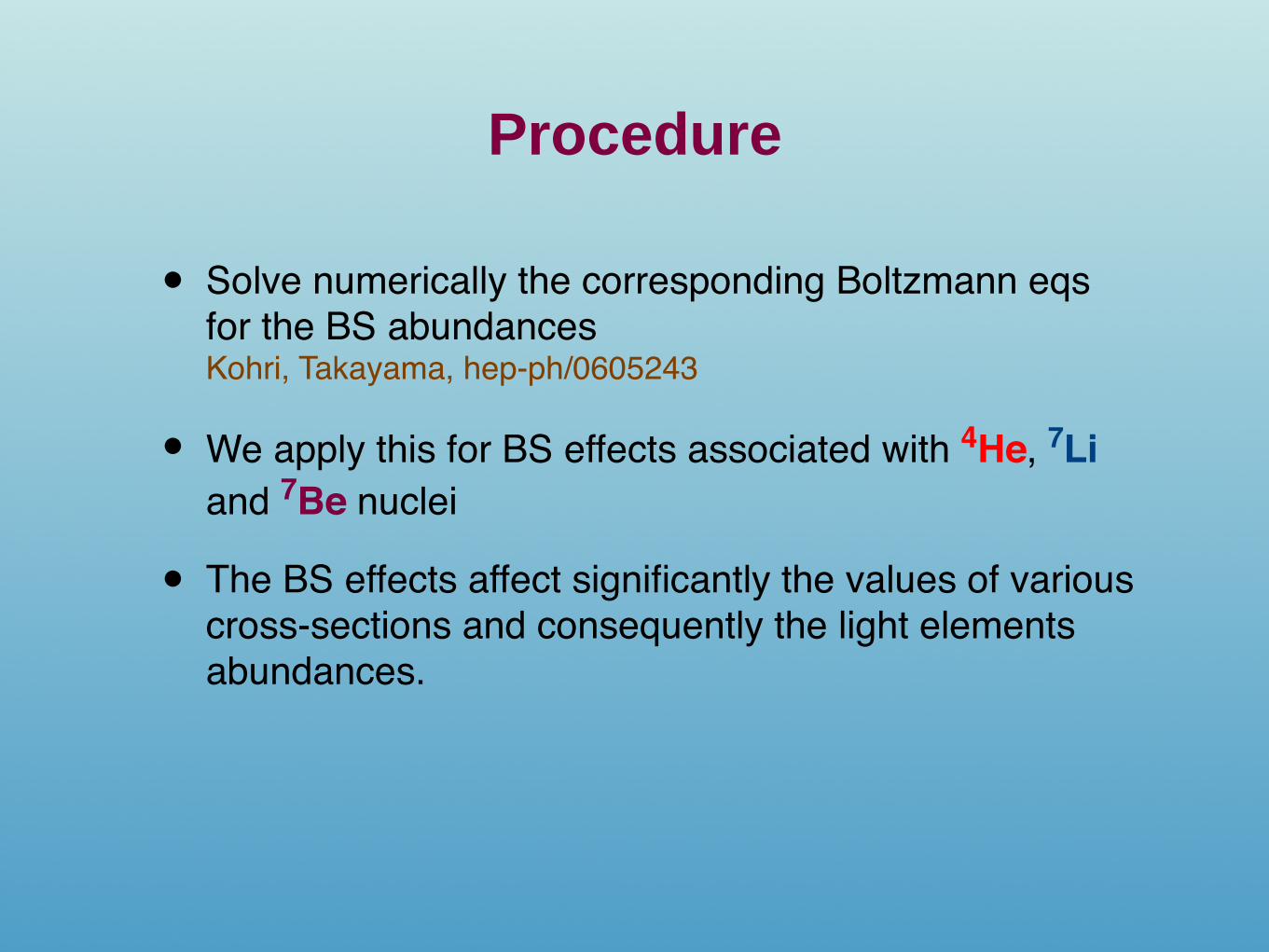
Procedure
• Solve numerically the corresponding Boltzmann eqs for the BS abundances Kohri, Takayama, hep-ph/0605243
• We apply this for BS effects associated with 4He, 7Li and 7Be nuclei
• The BS effects affect significantly the values of various cross-sections and consequently the light elements abundances.
nuclear interactions, and it thus turns out that bound state formation results in catalysis of
nuclear rates via two mechanisms.
One immediate consequence of the bound states is a reduction of the Coulomb barrier for
nuclear reactions, due to partial screening by the stau. Since Coulomb repulsion dominates
the charged-particle rates, all such rates are enhanced. Specifically, for the case of an initial
state A1 + A2, Coulomb effects lead to a exponential suppression via a penetration factor
which scales as Z2/31 Z2/3
2 A1/3, with A = A1A2/(A1 + A2). Introduction of a bound state
(τ , A2) decreases the target charge to Z2 − 1 and the system’s reduced mass number to
A = A1; both effects lower the Coulomb suppression. We include these effects for all reactions
with bound states.
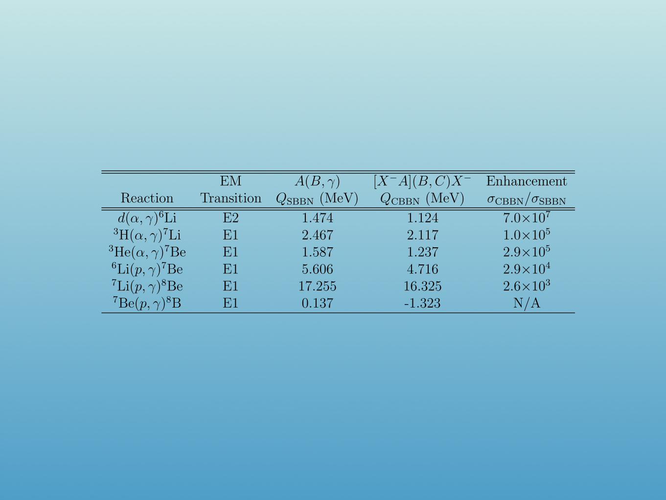
Table 1: Bound-state virtual photon enhancements to radiative capture cross sections forvarious reactions. The third (fourth) column is the threshold energy for the standard (cat-alyzed) BBN. The last column is the virtual photon enhancement factor of the catalyzed crosssection relative to standard BBN.
EM A(B, γ) [X−A](B, C)X− EnhancementReaction Transition QSBBN (MeV) QCBBN (MeV) σCBBN/σSBBN
d(α, γ)6Li E2 1.474 1.124 7.0×10⁷
3H(α, γ)7Li E1 2.467 2.117 1.0×10⁵
3He(α, γ)7Be E1 1.587 1.237 2.9×10⁵
6Li(p, γ)7Be E1 5.606 4.716 2.9×10⁴
7Li(p, γ)8Be E1 17.255 16.325 2.6×10³
7Be(p, γ)8B E1 0.137 -1.323 N/A
An additional effect enhances radiative capture channels A2(A1, γ)X by introducing pho-
tonless final states in which the stau carries off the reaction energy transmitted via virtual
photon processes. In particular, the 4He(d, γ)6Li reaction, which is suppressed in standard
BBN, is enhanced by many orders of magnitude by the presence of the bound states. As
described in [30], the virtual photon channel has a cross section which is enhanced over that
of the usual radiative capture cross section by
σCBBN
σSBBN∼ (aω)−n, (7)
where a is the BS Bohr radius and ω = λ−1 is the photon energy. The index n depends on
the type of transition multipole: for (E1,E2) transitions, n = (3, 5). Large enhancements of
this type affect other radiative capture reactions, notably mass-7 production reactions such
9
100 1000 2000 3000 4000 5000
0
1000
2000
100 1000 2000 3000 4000 5000
0
1000
2000
4.0D = 4.02.2
3He/D = 17
Li = 4.3
6Li/7
Li = 0.15 0.01
0.15
m0 (
GeV
)
m1/2 (GeV)
m3/2 = 100 GeV , tan ! = 10 , µ > 0
100 1000 2000 3000 4000 5000
0
1000
2000
100 1000 2000 3000 4000 5000
0
1000
2000
7Li = 4.3
6Li/7
Li = 0.15 0.01
4.0D = 4.02.2
m0 (
GeV
)
m1/2 (GeV)
m3/2 = 100 GeV , tan ! = 10 , µ > 0
4.3
100 1000 2000 3000 4000 5000
0
1000
2000
100 1000 2000 3000 4000 5000
0
1000
2000
D = 4.0
7Li = 4.3 6
Li/7Li = 0.15
0.01m0 (
GeV
)
m1/2 (GeV)
m3/2 = 0.2m0 , tan ! = 10 , µ > 0
100 1000 2000 3000 4000 5000
0
1000
2000
1
100 1000 2000 3000 4000 5000
0
1000
2000
D = 4.0
7Li = 4.3
6Li/7
Li = 0.150.01
m0 (
GeV
)
m1/2 (GeV)
m3/2 = 0.2m0 , tan ! = 10 , µ > 0
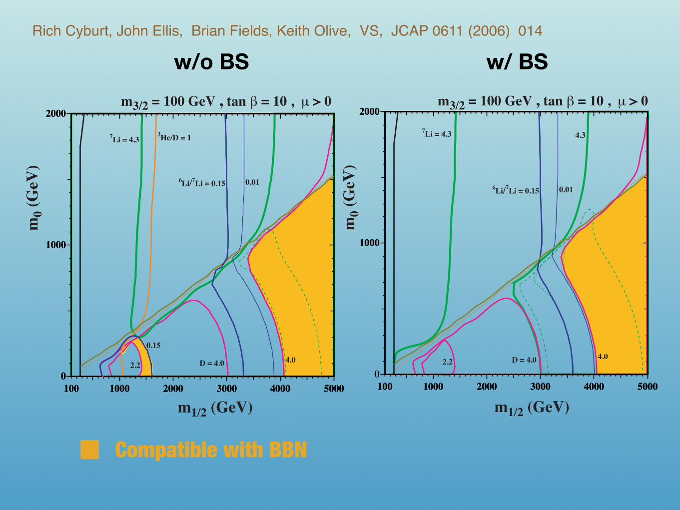
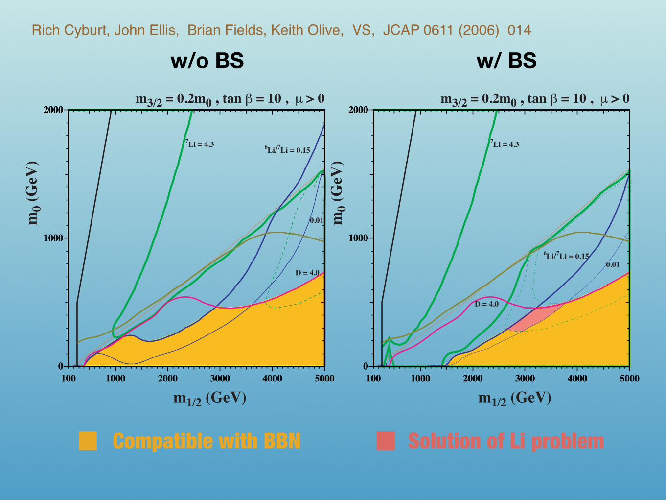
Figure 2: Some (m1/2, m0) planes for A0 = 0, µ > 0 and tanβ = 10. In the upper (lower)panels we use m3/2 = 100 GeV (m3/2 = 0.2 m0). In the right panels the effects of the staubound states have been included, while in those on the left we include only the effect of theNSP decays. The regions to the left of the solid black lines are not considered, since therethe gravitino is not the LSP. In the orange (light) shaded regions, the differences betweenthe calculated and observed light-element abundances are no greater than in standard BBNwithout late particle decays. In the pink (dark) shaded region in panel d, the abundances liewithin the ranges favoured by observation, as described in the text. The significances of theother lines and contours are explained in the text.
12
w/o BS w/ BS
Compatible with BBN
Rich Cyburt, John Ellis, Brian Fields, Keith Olive, VS, JCAP 0611 (2006) 014
100 1000 2000 3000 4000 5000
0
1000
2000
100 1000 2000 3000 4000 5000
0
1000
2000
4.0D = 4.02.2
3He/D = 17
Li = 4.3
6Li/7
Li = 0.15 0.01
0.15
m0 (
GeV
)
m1/2 (GeV)
m3/2 = 100 GeV , tan ! = 10 , µ > 0
100 1000 2000 3000 4000 5000
0
1000
2000
100 1000 2000 3000 4000 5000
0
1000
2000
7Li = 4.3
6Li/7
Li = 0.15 0.01
4.0D = 4.02.2
m0 (
GeV
)
m1/2 (GeV)
m3/2 = 100 GeV , tan ! = 10 , µ > 0
4.3
100 1000 2000 3000 4000 5000
0
1000
2000
100 1000 2000 3000 4000 5000
0
1000
2000
D = 4.0
7Li = 4.3 6
Li/7Li = 0.15
0.01m0 (
GeV
)
m1/2 (GeV)
m3/2 = 0.2m0 , tan ! = 10 , µ > 0
100 1000 2000 3000 4000 5000
0
1000
2000
1
100 1000 2000 3000 4000 5000
0
1000
2000
D = 4.0
7Li = 4.3
6Li/7
Li = 0.150.01
m0 (
GeV
)
m1/2 (GeV)
m3/2 = 0.2m0 , tan ! = 10 , µ > 0
Figure 2: Some (m1/2, m0) planes for A0 = 0, µ > 0 and tanβ = 10. In the upper (lower)panels we use m3/2 = 100 GeV (m3/2 = 0.2 m0). In the right panels the effects of the staubound states have been included, while in those on the left we include only the effect of theNSP decays. The regions to the left of the solid black lines are not considered, since therethe gravitino is not the LSP. In the orange (light) shaded regions, the differences betweenthe calculated and observed light-element abundances are no greater than in standard BBNwithout late particle decays. In the pink (dark) shaded region in panel d, the abundances liewithin the ranges favoured by observation, as described in the text. The significances of theother lines and contours are explained in the text.
12
w/o BS w/ BS
Compatible with BBN Solution of Li problem
Rich Cyburt, John Ellis, Brian Fields, Keith Olive, VS, JCAP 0611 (2006) 014
7Li = 4.3
0.01
m0 (
GeV
)
m1/2 (GeV)
m3/2 = 0.2m0 , tan ! = 57 , µ > 0
100 1000 2000 3000 4000 5000
0
1000
2000
3000
00
100 1000 2000 3000 4000 5000
0
1000
2000
3000
D = 4.0
6Li/7
Li = 0.15
0.01
100 1000 2000 3000 4000 5000
0
1000
2000
3000
100 1000 2000 3000 4000 5000
0
1000
2000
3000
m0 (
GeV
)
m1/2 (GeV)
m3/2 = 0.2m0 , tan ! = 57 , µ > 0
7Li = 4.3
6Li/7
Li = 0.15
0.15
0.01
7Li = 4.3
D = 4.0
100 1000 2000 3000 4000 5000
0
1000
2000
3000
100 1000 2000 3000 4000 5000
0
1000
2000
3000
D = 4.0
2.2
3He/D = 1
7Li = 4.3
6Li/7
Li = 0.15
0.01
0.15
m0 (
GeV
)
m1/2 (GeV)
m3/2 = m0, A0 = 3 - "3, µ > 0
100 1000 2000 3000 4000 5000
0
1000
2000
3000
100 1000 2000 3000 4000 5000
0
1000
2000
3000
D = 4.0
2.2
7Li = 4.3
m0 (
GeV
)
m1/2 (GeV)
m3/2 = m0, A0 = 3 - "3, µ > 0
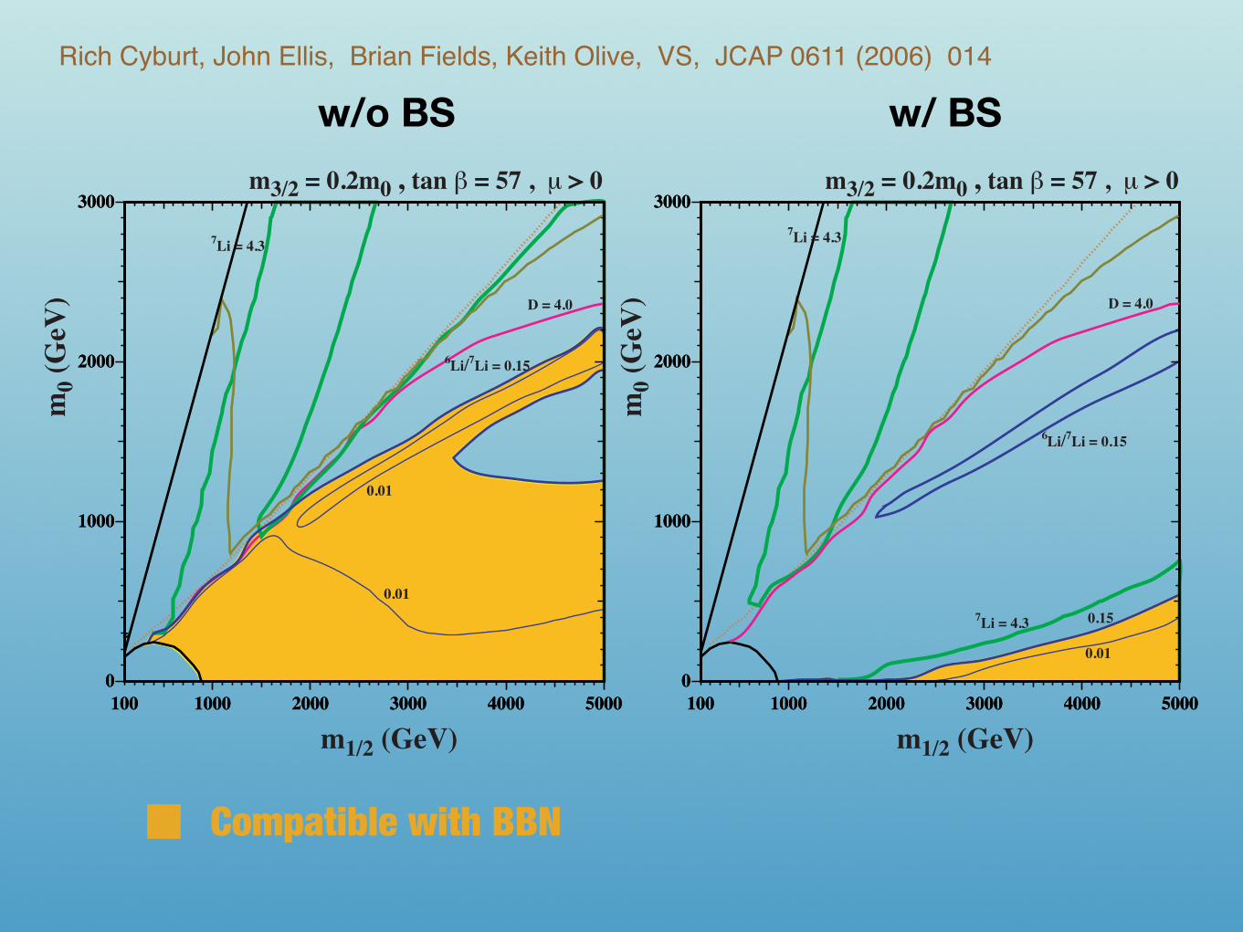
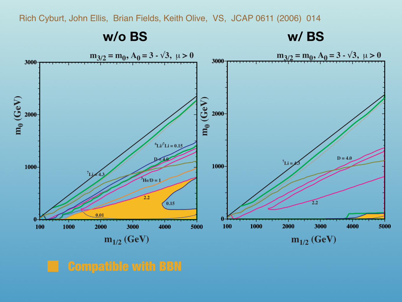
Figure 3: Some more (m1/2, m0) planes for µ > 0. In the upper panels we use m3/2 = 0.2 m0
and tanβ = 57, whilst in the lower panels we assume mSUGRA with m3/2 = m0 andA0/m0 = 3 −
√3 as in the simplest Polonyi superpotential. In the right panels the effects of
the stau bound states have been included, while in those on the left we include only the effectsof the NSP decays. As in Fig. 2, the region above the solid black line is excluded, sincethere the gravitino is not the LSP. In the orange shaded regions, the differences betweenthe calculated and observed light-element abundances are no greater than in standard BBNwithout late particle decays. The meanings of the other lines and contours are explained inthe text.
16
w/o BS w/ BS
Compatible with BBN
Rich Cyburt, John Ellis, Brian Fields, Keith Olive, VS, JCAP 0611 (2006) 014
7Li = 4.3
0.01
m0 (
GeV
)
m1/2 (GeV)
m3/2 = 0.2m0 , tan ! = 57 , µ > 0
100 1000 2000 3000 4000 5000
0
1000
2000
3000
00
100 1000 2000 3000 4000 5000
0
1000
2000
3000
D = 4.0
6Li/7
Li = 0.15
0.01
100 1000 2000 3000 4000 5000
0
1000
2000
3000
100 1000 2000 3000 4000 5000
0
1000
2000
3000
m0 (
GeV
)
m1/2 (GeV)
m3/2 = 0.2m0 , tan ! = 57 , µ > 0
7Li = 4.3
6Li/7
Li = 0.15
0.15
0.01
7Li = 4.3
D = 4.0
100 1000 2000 3000 4000 5000
0
1000
2000
3000
100 1000 2000 3000 4000 5000
0
1000
2000
3000
D = 4.0
2.2
3He/D = 1
7Li = 4.3
6Li/7
Li = 0.15
0.01
0.15
m0 (
GeV
)
m1/2 (GeV)
m3/2 = m0, A0 = 3 - "3, µ > 0
100 1000 2000 3000 4000 5000
0
1000
2000
3000
100 1000 2000 3000 4000 5000
0
1000
2000
3000
D = 4.0
2.2
7Li = 4.3
m0 (
GeV
)
m1/2 (GeV)
m3/2 = m0, A0 = 3 - "3, µ > 0
Figure 3: Some more (m1/2, m0) planes for µ > 0. In the upper panels we use m3/2 = 0.2 m0
and tanβ = 57, whilst in the lower panels we assume mSUGRA with m3/2 = m0 andA0/m0 = 3 −
√3 as in the simplest Polonyi superpotential. In the right panels the effects of
the stau bound states have been included, while in those on the left we include only the effectsof the NSP decays. As in Fig. 2, the region above the solid black line is excluded, sincethere the gravitino is not the LSP. In the orange shaded regions, the differences betweenthe calculated and observed light-element abundances are no greater than in standard BBNwithout late particle decays. The meanings of the other lines and contours are explained inthe text.
16
w/o BS w/ BS
Compatible with BBN
Rich Cyburt, John Ellis, Brian Fields, Keith Olive, VS, JCAP 0611 (2006) 014
Summary-Prospects We present a new BBN calculation including the effects of the EM and HD decays of the NSP
Including the bound-states effects in the stau NSP case
NSP decays probably can not solve the lithium problem
The bound states effects for the stau NSP case are important and exclude regions of the parameter space with lifetimes longer than 10 4 s. But can explain the lithium isotopes discrepancies for τ ≲1000 s can!
More work to be done: detailed scan of the parameter space SUSY searches at LHC effects on the A=5,8 bottlenecks etc
Unstable gravitino effects of neutralino DM models (w/ R. Cyburt, J. Ellis, K. Olive, B. Fields)


![THE HIGGS PORTAL TO DARK MATTER AT THE LHC · THE “WIMP’’ MIRACLE 4 Relic dark matter abundance after thermal freeze-out: [Planck coll. 2015, arXiv:1502.01589] h Avi =3⇥ 1026cm3s1](https://img.pdfslide.net/doc/110x75/5fa71b5c0be2995af04af945/the-higgs-portal-to-dark-matter-at-the-lhc-the-aoewimpaa-miracle-4-relic-dark.jpg)

![Leszek Roszkowski, Sebastian Trojanowski, Krzysztof … · arXiv:1406.0012v2 [hep-ph] 3 Oct 2014 Neutralino and gravitino dark matter with low reheating temperature Leszek Roszkowski,a1](https://img.pdfslide.net/doc/110x75/5aeb56fc7f8b9a3b2e8dd877/leszek-roszkowski-sebastian-trojanowski-krzysztof-14060012v2-hep-ph-3-oct.jpg)