Embed Size (px)
Citation preview
R. B. King GLFWRA Final Report 30 Sept 2013
1
Great Lakes Fish and Wildlife Restoration Act FINAL Project Report
Project Title: PREDICTING CLIMATE‐CHANGE INDUCED DISTRIBUTIONAL SHIFTS IN GREAT LAKES REGION REPTILES Project Sponsor: Illinois DNR FWS Agreement Number: 30181AG189 Principal Investigator(s): Richard B. King Report Author(s): Richard B. King; Methods and Results coauthored by Michael L. Niiro Date Submitted: 30 September 2013 Study Objectives: The objectives of this study are to use the maximum entropy method of ecological niche modeling to (1) characterize the association between climatic variables and the current distributions of reptiles of conservation concern in the Great Lakes region, (2) use this information to identify the projected future location of areas of high climatic suitability, and (3) prioritize species and associated management, research, and policy actions based on these projections List of presentations delivered and outreach activities: Niiro, M., and King, R. Midwest Partners in Amphibian and Reptile Conservation Annual
Meeting, "Predicting Climate‐Change Induced Distributional Shifts in Great Lakes Region Reptiles," Pioneer, OH. (2012).
Niiro, M., and King, R. 7th World Congress of Herpetology, "Predicting Climate‐Change Induced Distributional Shifts in Great Lakes Region Reptiles," Vancouver, BC. (2012).
Niiro, M., And King, R. International Biogeography Society meeting, “Predicting Future Climatic Suitability for Great Lakes Region Reptiles Using the Maximum Entropy Approach,” Miami, FL (2013).
Geographic region project occurred in or effects: Great Lakes region; Minnesota, Illinois, Wisconsin, Indiana, Michigan, Ohio, Pennsylvania, New York and surrounding states and Canadian Provinces List of reports and peer‐reviewed papers completed or in‐progress: Copies of this report will be provided to institutions, agencies and personnel listed in Table 1 and to other relevant agencies within the states and provinces included in this study. The work described here will form the basis of an MS thesis by M. Niiro (anticipated fall, 2013) and a manuscript submitted for publication in an appropriate peer‐reviewed journal (e.g., Diversity and Distributions, Ecography, Journal of Biogeography).
R. B. King GLFWRA Final Report 30 Sept 2013
2
Executive Summary/Abstract for Project: Climate change is widely recognized as an imminent threat to native flora and fauna but efforts to address this threat are only beginning. As a group, reptiles may be especially subject to the effects of climate change – their active season is limited by length of the frost‐free period and successful reproduction requires access to suitable thermal microhabitats during gestation or incubation. Within the Great Lakes region, mean temperature is expected to increase by ca. 2 degrees C and mean rainfall is expected to increase by ca. 0.2 mm per day by 2060. Among Great Lakes region reptiles are seven snakes and five turtles that are of conservation concern and whose distributions are largely restricted to or broadly encompass the region. The objectives of this study are to use the maximum entropy method of ecological niche modeling to (1) characterize the association between climatic variables and the current distributions of reptiles of conservation concern in the Great Lakes region, (2) use this information to identify the projected future location of areas of high climatic suitability, and (3) prioritize species and associated management, research, and policy actions based on these projections. Current distributions of reptiles of conservation concern in the Great Lakes region were well predicted by ecological niche models that incorporated four to seven climatic variables. These species consistently showed projected reductions in climatic suitability at locations currently occupied and most showed reductions in climatic suitability within the region more generally. Projected reductions in climatic suitability first became evident in southern and western portions of species’ ranges. Reptile species of conservation concern in the Great Lakes region differed in their susceptibility to climate change. Butler’s Gartersnake, Eastern and Western Foxsnakes, and Short‐headed Gartersnake were least sensitive to climate change; greater than 75% of their known localities were projected to remain climatically suitable in 2050 using the maximum sum of sensitivity and specificity threshold. Furthermore, these species may benefit from the appearance of new areas of high climatic suitability that are not currently occupied. The Spotted Turtle and Northern Map Turtle were somewhat more sensitive; 50‐75% of known localities were projected to remain climatically suitable. The remaining species appeared to be more highly sensitive to climate change. Blanding’s Turtle, Eastern Massasauga, and Queensnake were projected to have 25‐50% of known localities remain climatically suitable and Kirtland’s Snake, Wood Turtle, and Bog Turtle were projected to have less than 25% of known localities remain climatically suitable. High priority species for management, research, and policy actions in response to the threat posed by climate change include Blanding’s Turtle, Eastern Massasauga, Queensnake, Kirtland’s Snake, Wood Turtle, and Bog Turtle. Management actions include population monitoring especially in areas of decreasing climatic suitability, habitat enhancement, identification and establishment of corridors among habitat fragments, and possible ‘rescue’ of doomed populations for captive breeding or translocation. Research actions include population viability analysis within areas of decreasing climatic suitability and assessments of colonization ability of newly suitable areas. Policy actions include evaluations of the need for greater legal protection, expanded critical habitat designation, and modified habitat management plans.
R. B. King GLFWRA Final Report 30 Sept 2013
3
Introduction Climate change is widely recognized as an imminent threat to native flora and fauna (Thomas et al. 2004; Ackerly et al. 2010), but efforts to address this threat are only beginning. For example, just 10% of USFWS recovery plans identify climate change as a threat (124 of 1209 species recovery plans) and only 15 offer substantive analysis of this threat and possible mitigation (Povilitis and Sucklin 2009). Because of the rapidity with which climate change is expected to impact native species (Thomas et al. 2004), analytical methods that allow swift prioritization of species and associated management, research, and policy actions will allow managers and policy makers to address climate change impacts in a time‐ and cost‐effective manner. While the threats imposed by habitat loss, overexploitation, and invasive species are considerable, their resolution typically involves strategies focused on populations within known geographic regions. In contrast, climate change may result in significant shifts in the geographic distribution of environmental conditions suitable for population persistence and as a consequence, management strategies will additionally need to focus on areas not currently occupied by species of concern. The urgency with which climate change impacts need to be addressed is underscored by the observation that pole‐ward shifts in species’ boundaries are already evident in many species; of 329 animal taxa, an excess of 68% showed distributional shifts consistent with climate change over the 25 years preceding 2000 (Hickling et al. 2006; Thomas 2010). As a group, reptiles may be especially subject to the effects of climate change – their active season is limited by length of the frost‐free period and successful reproduction requires access to suitable thermal microhabitats during gestation or incubation (Deutsch et al. 2008; Doody and Moore 2010). Physiological processes are temperature‐dependent (Huey 1982), as is sex determination in many species, particularly turtles (Ewert and Nelson 1991). Furthermore, limited dispersal ability may prevent some reptile species from naturally colonizing new habitats (Araújo and Pearson, 2005). Within the Great Lakes region, mean temperature is expected to increase by ca. 2 degrees C and mean rainfall is expected to increase by ca. 0.2 mm per day by 2060 (Galatowitsch et al. 2009). Already, climate change is resulting in shifting distributional patterns (e.g., among small mammals, Francl et al. 2010; Myers et al. 2009) and changes in phenology (e.g., among amphibians Brodman 2009; Klaus and Lougheed 2013). Among Great Lakes region reptiles are seven species of snakes and five species of turtles which are of conservation concern and whose distributions are largely restricted to or broadly encompass the region (Figure 1). Most of these species make extensive use of both wetland and upland habitat and have been negatively impacted by habitat loss and degradation resulting from wetland drainage, agriculture, and urbanization (Harding 1997). As a consequence, over much of their range, these species persist in small populations isolated from conspecifics by habitat fragmentation (Bennett et al. 2010; Congdon et al. 2008; Dileo et al. 2010; Shepard et al. 2008; Shoemaker et al. 2013; Willoughby et al. 2013). The availability of detailed information on species occurrence (e.g., georeferenced locality data from specimen repositories) and local climate (e.g., from NOAA recording stations) makes it
R. B. King GLFWRA Final Report 30 Sept 2013
4
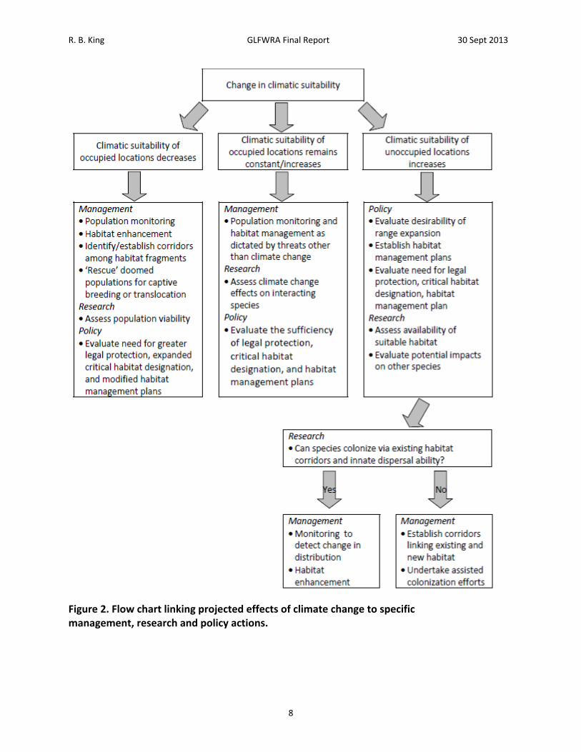
possible to characterize associations between current species distributions and individual or composite climate variables. Furthermore, this association can be used in conjunction with climate change projections to predict changes in the location of climatically suitable conditions into the future (e.g., Hijmans et al 2005; Hijmans and Graham2006; Penman et al. 2010; Phillips et al. 2006).). A variety of approaches have been developed for this purpose, (variously referred to as Climate Matching, Climate Envelope Modeling, Ecological Niche Modeling, or Species Distribtuion Modeling) and refinements to both the analytical techniques and the interpretation of results are emerging rapidly (e.g., Franklin 2010; Mateo et al. 2010; Tingley and Herman 2009; Thuiller et al. 2009). The objectives of this study are to use the maximum entropy method of ecological niche modeling to (1) characterize the association between climatic variables and the current distributions of reptiles of conservation concern in the Great Lakes region, (2) use this information to identify the projected future location of areas of high climatic suitability, and (3) prioritize species and associated management, research, and policy actions based on these projections. Climate change may affect Great Lakes region reptiles in different ways. Among species that have restricted distributions, and thus experience a narrow range of climatic conditions, future areas of high climatic suitability may occur in entirely new areas. In this study, such species are represented by the Short‐headed Gartersnake, Butler’s Gartersnake, and Kirtland’s Snake; species whose present distributions encompass portions of just three to seven states and provinces; and the Bog Turtle, a species that occurs within and outside the Great Lakes region but in disjunct areas (Figure 1). For more widely distributed species, future areas of high climatic suitability are more likely to overlap at least part of their current range. However, areas of high climatic suitability may contract, expand, shift in position, or become fragmented. Among the reptiles included here, Eastern and Western Foxsnakes (analyzed as a single entity as explained below), Eastern Massasauga, and Blanding’s Turtle are widely distributed within the Great Lakes region but have restricted distributions outside the region (Figure 1). Four other species, the Wood Turtle, Queen Snake, Common Map Turtle, Spotted Turtle, are widely distributed both within and outside the Great Lakes region (Figure 1). Thus, these species provide a test of the way in which current distribution might affect projected impacts of climate change. More importantly, projected changes in climatic suitability have immediate implications for management, research, and policy actions (Schwartz 2012; Figure 2). For species and areas for which climatic suitability of occupied locations remains constant or increases, management efforts designed to address threats other than climate change (habitat loss, overexploitation, invasive species) are appropriate. Research needs include an evaluation of climate change effects on key interacting species to identify possible indirect effects on species of conservation concern (e.g., prey specialists such as queen snakes are likely to be affected by climate change effects on crawfish). Policy needs include evaluation of the sufficiency of legal protection, critical habitat designation, and habitat management plans, given changes in climatic suitability elsewhere.
R. B. King GLFWRA Final Report 30 Sept 2013
5
For species and areas for which climatic suitability of occupied locations decreases, efforts that also address climate change are warranted (Figure 2). Management needs include population monitoring to facilitate rapid detection of climate change‐induced declines and habitat enhancement aimed at increasing local population size and reducing extinction risk. Establishment or enhancement of habitat corridors may be necessary to maintain demographic and genetic health of increasingly subdivided populations (i.e., ‘genetic restoration’, Hedrick 2005). If populations become too isolated for habitat corridors to be effective, facilitated movement of individuals among population subunits (reciprocal translocation) may be warranted. In the extreme, populations undergoing climate‐change induced declines might be targeted for ‘rescue’ via translocation of individuals to more suitable locations or incorporation into captive breeding programs as insurance against extinction and to provide stock of reintroduction or population augmentation. Research needs include population viability analysis (e.g., Enneson and Litzgus 2009) to assess risk of local extinction, thus informing the need for more active habitat management, translocation, or rescue. Policy needs include evaluation of the need for greater legal protection, expanded critical habitat designation, and modified habitat management plans. For species and areas for which climatic suitability of unoccupied locations increases, novel policy and research needs arise which take precedence over management (Figure 2). Specifically, the desirability of a conservation policy that includes range expansion needs to be evaluated in light of species status elsewhere and research on availability of suitable habitat within unoccupied areas (e.g., Suzuki et al. 2008, Tigley and Herman 2009) and the potential impacts (both positive and negative) of range expansion on other species (Roemer et al. 2002). This may lead to new policies regarding legal protection, critical habitat designations, and habitat conservation plans. It may also require research to address the potential for natural vs. assisted colonization (Bennie et al. 2013; Travis et al. 2013). Subsequent management needs could include monitoring efforts designed to track changes in distribution, possibly coupled with establishment or enhancement of habitat corridors and assisted colonization efforts (via translocation of individuals from existing populations; Chauvenet et al. 2012;Shirey and Lamberti 2009).
R. B. King GLFWRA Final Report 30 Sept 2013
6
State/
Province
Short‐headed
Gartersnake Butler's
Gartersnake Kirtland's Snake
Eastern/ Western Foxsnake
Eastern Massasauga
Bog Turtle
Blanding's Turtle
Wood Turtle
Queen‐ Snake
Northern Map Turtle
Spotted Turtle
SD +1 + NE +1 S2 KS T IA +1 E T E + MO S +1 3 E + AR + +
Great Lakes Region
MN +1 E T T + IL T +1 E E + + E WI T4 +1 E T4 T E + IN E E +1 E E + + E MI + E S5 S S S S + T OH S + T S5 E T S + T PA + E E E S + + + + NY + E E T S E + S ON E E5 T T E E S E QU S S S S
NB + NS E T KY + + + TN T + + WV S + S S VA E T + + + ME E + T NH E + T VT S S E MA E T S + RI S S CT E S + NJ E T E + + DE E + + + MD T + + E + NC T + + SC T + T GA E + S S AL + + FL + +
E Endangered T Threatened S Special Concern/Greatest Conservation Need + Present but no special status 1 Formerly designated Western Foxsnake 2 Tier 1 at‐risk species, Panella 2012 3 Extant Massasauga populations in Missouri are S. c. tergeminus (Gibbs et al. 2010, Kubatko et al. 2011, Ray et al. 2013) 4 Administrative rule process is underway to delist Blanding's Turtles and Butler's Gartersnakes in Wisconsin 5 Formerly designated Eastern Foxsnake
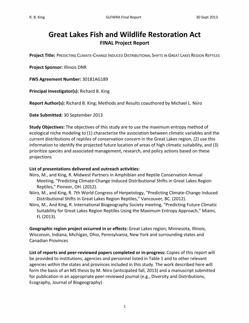
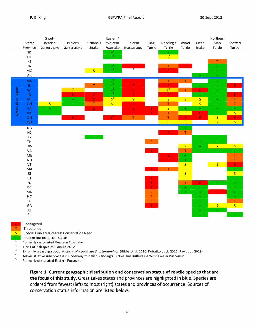
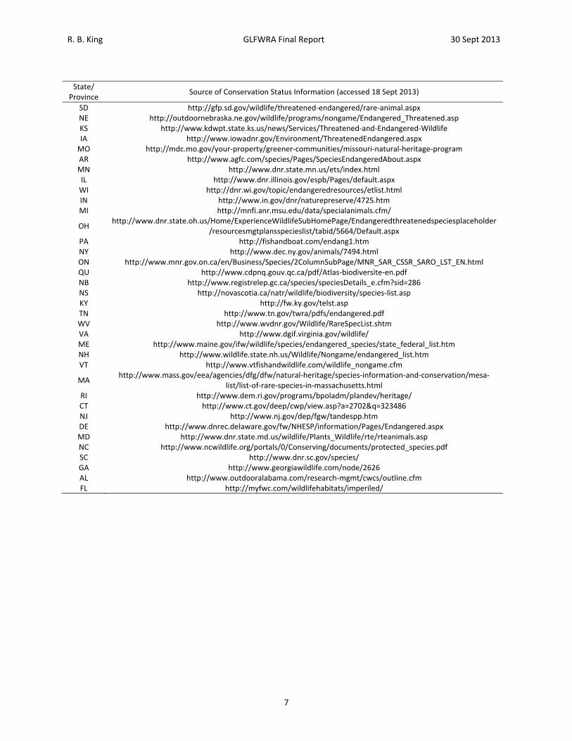
Figure 1. Current geographic distribution and conservation status of reptile species that are the focus of this study. Great Lakes states and provinces are highlighted in blue. Species are ordered from fewest (left) to most (right) states and provinces of occurrence. Sources of conservation status information are listed below.
R. B. King GLFWRA Final Report 30 Sept 2013
7
State/
Province Source of Conservation Status Information (accessed 18 Sept 2013)
SD http://gfp.sd.gov/wildlife/threatened‐endangered/rare‐animal.aspx NE http://outdoornebraska.ne.gov/wildlife/programs/nongame/Endangered_Threatened.asp KS http://www.kdwpt.state.ks.us/news/Services/Threatened‐and‐Endangered‐Wildlife IA http://www.iowadnr.gov/Environment/ThreatenedEndangered.aspx MO http://mdc.mo.gov/your‐property/greener‐communities/missouri‐natural‐heritage‐program AR http://www.agfc.com/species/Pages/SpeciesEndangeredAbout.aspx MN http://www.dnr.state.mn.us/ets/index.html IL http://www.dnr.illinois.gov/espb/Pages/default.aspx WI http://dnr.wi.gov/topic/endangeredresources/etlist.html IN http://www.in.gov/dnr/naturepreserve/4725.htm MI http://mnfi.anr.msu.edu/data/specialanimals.cfm/
OH http://www.dnr.state.oh.us/Home/ExperienceWildlifeSubHomePage/Endangeredthreatenedspeciesplaceholder
/resourcesmgtplansspecieslist/tabid/5664/Default.aspx PA http://fishandboat.com/endang1.htm NY http://www.dec.ny.gov/animals/7494.html ON http://www.mnr.gov.on.ca/en/Business/Species/2ColumnSubPage/MNR_SAR_CSSR_SARO_LST_EN.html QU http://www.cdpnq.gouv.qc.ca/pdf/Atlas‐biodiversite‐en.pdf NB http://www.registrelep.gc.ca/species/speciesDetails_e.cfm?sid=286 NS http://novascotia.ca/natr/wildlife/biodiversity/species‐list.asp KY http://fw.ky.gov/telst.asp TN http://www.tn.gov/twra/pdfs/endangered.pdf WV http://www.wvdnr.gov/Wildlife/RareSpecList.shtm VA http://www.dgif.virginia.gov/wildlife/ ME http://www.maine.gov/ifw/wildlife/species/endangered_species/state_federal_list.htm NH http://www.wildlife.state.nh.us/Wildlife/Nongame/endangered_list.htm VT http://www.vtfishandwildlife.com/wildlife_nongame.cfm
MA http://www.mass.gov/eea/agencies/dfg/dfw/natural‐heritage/species‐information‐and‐conservation/mesa‐
list/list‐of‐rare‐species‐in‐massachusetts.html RI http://www.dem.ri.gov/programs/bpoladm/plandev/heritage/ CT http://www.ct.gov/deep/cwp/view.asp?a=2702&q=323486 NJ http://www.nj.gov/dep/fgw/tandespp.htm DE http://www.dnrec.delaware.gov/fw/NHESP/information/Pages/Endangered.aspx MD http://www.dnr.state.md.us/wildlife/Plants_Wildlife/rte/rteanimals.asp NC http://www.ncwildlife.org/portals/0/Conserving/documents/protected_species.pdf SC http://www.dnr.sc.gov/species/ GA http://www.georgiawildlife.com/node/2626 AL http://www.outdooralabama.com/research‐mgmt/cwcs/outline.cfm FL http://myfwc.com/wildlifehabitats/imperiled/
R. B. King GLFWRA Final Report 30 Sept 2013
8
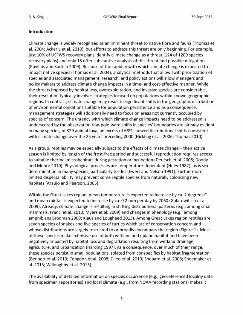
Figure 2. Flow chart linking projected effects of climate change to specific management, research and policy actions.
R. B. King GLFWRA Final Report 30 Sept 2013
9
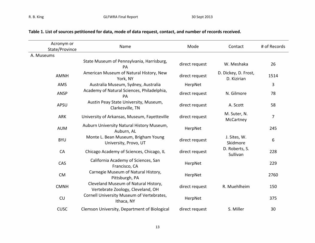
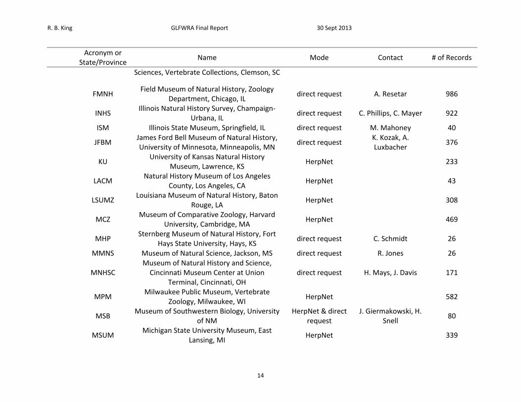
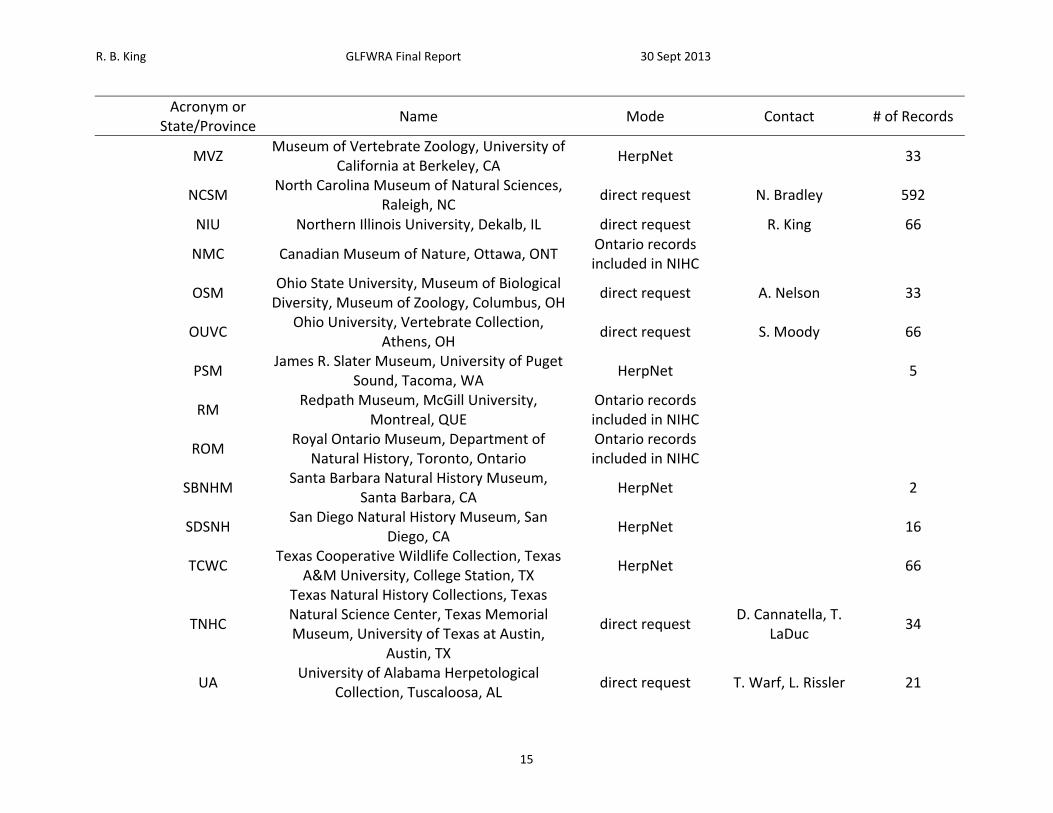
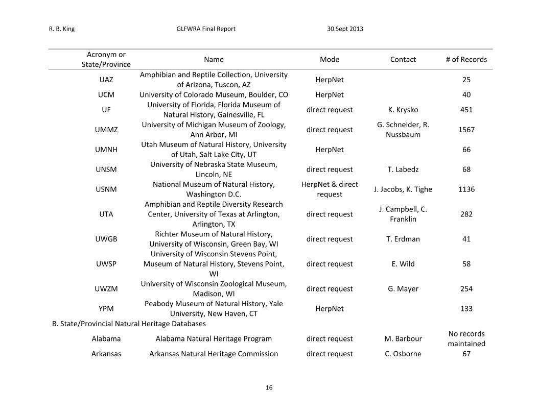
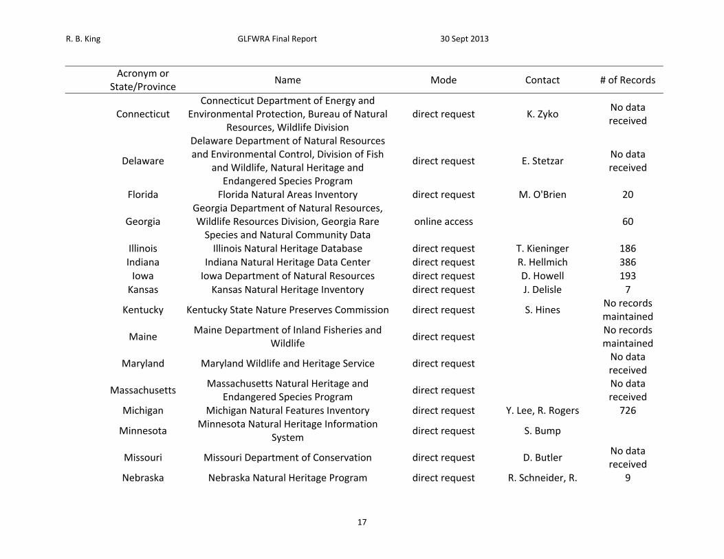
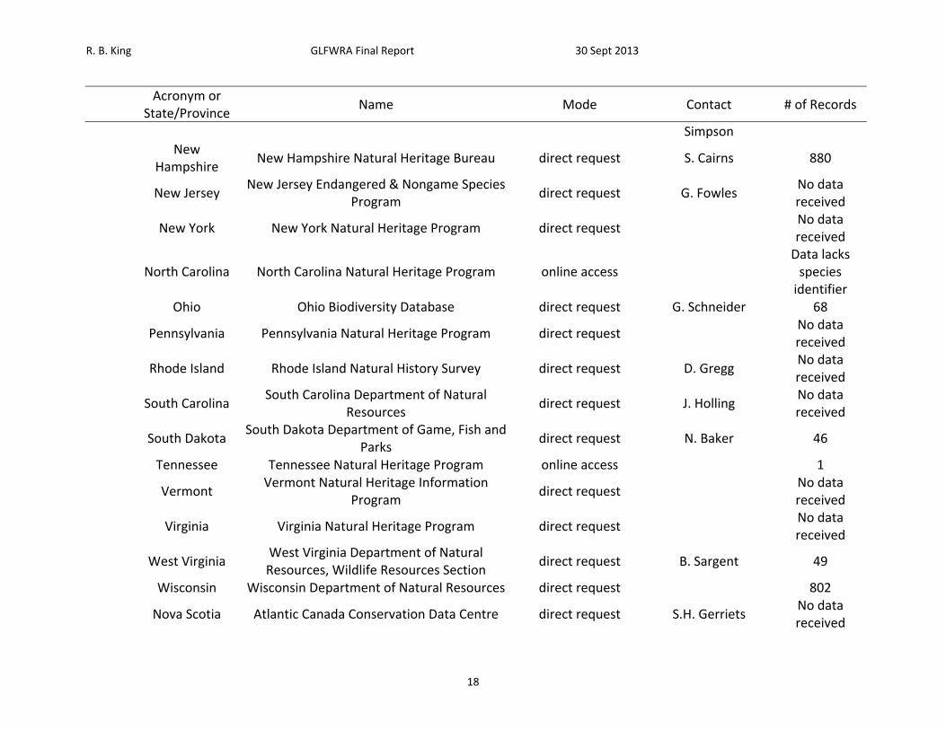
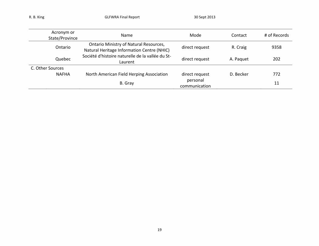
Methods Compilation of Georeferenced Locality Data. – Locality records were obtained through queries of the HerpNET network of herpetological collections (http://herpnet.org/) and requests to individual institutions and appropriate state and provincial agencies (e.g., Departments of Natural Resources) and other sources (Table 1). These records were compiled into a searchable database using FileMaker Pro 11. When necessary, geographic coordinates were generated from site descriptions using GeoLocate (http://www.museum.tulane.edu/geolocate/). Records georeferenced using GeoLocate were included only if their associated uncertainty was <10 km (a scale comparable to the spatial resolution of climatic data as described below). Records were mapped using ArcMap 10.1 (www.esri.com) and compared to regional distributional maps (e.g., state and regional field guides) to identify likely erroneous records for subsequent correction or exclusion. To control for possible search effort bias, spatial filtering of records was used to achieve a relatively uniform distribution (Kramer‐Schadt et al. 2013, Yackulic et al. 2012). This was accomplished by applying a grid with a square cell size of 15 arcminutes by 15 arcminutes. Within each grid cell, one record was randomly selected for inclusion in the analyses. An exception was made for the case of Thamnophis brachystoma where the cell size was 5 arcminutes by 5 arcminutes to account for this species’ limited distribution. Following spatial filtering, the number of records retained for analysis ranged from 89‐665 among species (Table 2) and exceeded sample size thresholds for acceptable model performance (Wisz et al. 2008). In general, each species was analyzed in a separate model with its own geographic background. An exception was made for the Eastern Foxsnake and Western Foxsnake, given recent changes in the taxonomy of these two species (Crother et al. 2011, Row et al. 2011). Previously, the Eastern Foxsnake and the Western Foxsnake were considered subspecies, and later distinct species that occupied disjunct geographic ranges (Collins 1991). The Western Foxsnake occurred in South Dakota, Nebraska, Minnesota, Iowa, Illinois, Wisconsin, the upper peninsula of Michigan, and western Indiana whereas the Eastern Foxsnake occurred in northern Ohio, eastern Michigan, and southern Ontario (Conant and Collins 1991). A gap of 250 km in eastern Indiana and western Ohio, where neither species was found, separated the species (Crother et al. 2011, Row et al. 2011). Recent molecular genetic analyses indicate that while two well differentiated Foxsnake clades do exist, their geographic distribution does not conform to previous species designations. These analyses suggest a species boundary and area of sympatry at the Mississippi River (Crother et al. 2011). Because this area of sympatry is poorly characterized and the two species cannot be fully distinguished using morphological characters (Crother et al. 2011), occurrence records could not be assigned unambiguously by species and so Eastern and Western Foxsnakes were pooled in one model. An exception was also made for the Massasauga Rattlesnake, Sistrurus catenatus, for which just the Eastern Massasauga, S. c. catenatus, was modeled based on its disjunct distribution (fig. 1 in Kubatko et al. 2011) and strong (species‐level) genetic differentiation from the Western Massasauga, S. c. tergeminus (Gibbs et al. 2010, Kubatko et al. 2011, Ray et al. 2013).
R. B. King GLFWRA Final Report 30 Sept 2013
10
Exceptions were also made in model construction for the Blanding’s Turtle and the Queensnake. Several disjunct populations of these species were excluded from the models to prevent undue influence on the geographic background. Blanding’s Turtles occur primarily in the northern states of the Midwestern region of the United States and the southern part of Ontario, Canada (Conant and Collins 1991). A disjunct population occurs in Massachusetts, Rhode Island, Vermont, New Hampshire and Connecticut, but it is separated from the next nearest occurrence by approximately 350 km. Another disjunct population is located in Nova Scotia and is separated from the next nearest occurrence by approximately 300 km. Genetic analyses indicate that these three geographic regions represent separate evolutionarily significant units (Mockford et al. 2007). Queensnakes are found throughout many of the states east of the Mississippi River from as far south as Florida to as far north as New York (Conant and Collins 1991). A disjunct population in Arkansas is separated from the next nearest occurrence by approximately 300 km. Although the Wood Turtle occurs in both New Brunswick and Nova Scotia, no records for this species were included in the data compilation and so these provinces were excluded from state/province specific summaries for this species. Model Implementation. – Models were implemented in MaxEnt, a maximum entropy modeling platform that makes use of species presence and background point data to identify environmental variables associated with species distribution (Phillips et al. 2006). The geographic extent from which points are selected in MaxEnt is important to the building of an accurate model (VanDerWal 2009, Rodda et al. 2011, Acevedo et al. 2012). An extent that is too large will result in a highly discriminatory model that is overfit to the data. An undersized extent will result in the model not discriminating at all and being highly underfit to the data. For each species, a buffer was placed around known occurrences and then combined these buffered occurrences into a single continuous polygon in ArcGIS to create the background extent. The resulting polygon was then used to clip the environmental layers in order to restrict the range from which MaxEnt selects its background points. As a default, MaxEnt uses 10,000 randomly selected background points unless the environmental layer has fewer than 10,000 points, in which case MaxEnt uses all points from the environmental layer. A variety of buffer sizes was tested to minimize the mismatch between the known distribution and the area of highest climatic suitability in the MaxEnt model (following VanDerWal et al. 2008). Based upon this testing, a buffer of 250 km provided the model with least mismatch across all species. Models were trained using climatic data from the WorldClim database representing the time period from 1950 to 2000 with a resolution of 5 arcminutes. At the latitudes of the target species, this corresponds to an approximately square area of ca. 9 km by 9 km. Models were run using 10‐fold cross‐validation. Under this method, the presence records are split into ten equal folds. Nine folds are used to train the model, and the tenth fold is used to evaluate the model. The model is trained ten times, each time using a different data fold as the tenth fold for evaluating the model. The models are then averaged to produce a final model. In the IPCC Third Assessment Report, a number of different greenhouse gas emissions scenarios were described in the Special Report on Emissions Scenarios (Special Report on Emissions Scenarios
R. B. King GLFWRA Final Report 30 Sept 2013
11
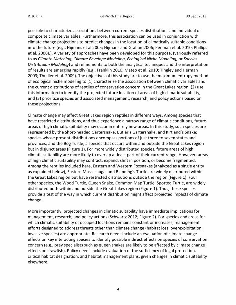
2000). These scenarios describe different assumptions about the forces driving climate change. There are 40 different scenarios organized into 4 major scenario families. The A1 and A2 scenario families assume a greater focus on economic development, and thus greater greenhouse gas emissions, whereas the B1 and B2 scenario families assume a greater focus on achieving sustainable practices, and thus comparatively lower greenhouse gas emissions. The A1 and B1 scenario families assume globalization, where new technologies spread rapidly between countries. The A2 and B2 scenario families assume greater regionalization, where development is focused locally and new technologies do not spread as rapidly. The A2a and B2a climate scenarios were selected, as these scenarios are frequently used in environmental niche model analyses (Ihlow et al. 2012, Warren and Seifert 2011). Two different climate scenarios were used to provide differing projections for climate change that better reflect the range of outcomes seen among the 40 climate scenarios from the Special Report on Emissions Scenarios. The data for the A2a and B2a climate scenarios were also more readily available in a variety of formats than the other climate scenarios. Downscaled GCM data from IPCC Fourth Assessment Report was downloaded from the International Center for Tropical Agriculture (CIAT) data portal (Jarvis 2008). Data were downloaded for the A2a and B2a scenarios for the years 2020, 2050, and 2080 from the Hadley Centre’s HadCM3, a coupled climate model. Selection of environmental variables is also an important contributor to model performance and the problem of overfitting (Rodda et al. 2011). A common method is to use the Bioclim variables, a set of 19 bioclimatic variables derived from monthly temperature and precipitation values (Table 3). This variable set was restricted as follows to reduce overfitting of the model (Rodda et al. 2011). Variables Bio8, Bio9, Bio18, and Bio19 were removed a priori due to sharp discontinuities that did not correspond with underlying geographic features (King and Niiro unpublished). ENMTools was used to calculate the Pearson correlation coefficient for each pairwise combination of BioClim variables within polygons generated as described above. For all pairwise correlations where |r|> 0.85, the variable with fewer strong correlations (|r|>0.85) was removed, starting with the highest pairwise correlation. The process was repeated until there were no strong correlations (|r| > 0.85) remaining among the selected variables (Elith et al. 2006). While some authors have used lower or higher correlation thresholds (Kumar and Stohlgren 2009, Fang et al. 2013), the use of 0.85 in this study resulted in retention of an intermediate number (4‐7; Table 4) of variables (a lower threshold would result in fewer retained variables, whereas a higher threshold would result in more variables) while maintaining moderate potential explanatory variation (1 – 0.852 = 0.28) as compared to a higher threshold (e.g., 1 – 0.902 = 0.19). Finally, model performance and overfitting are affected by the complexity of response functions allowed during model selection. This is controlled through the regularization parameter, frequently symbolized as β (Phillips and Dudik 2008, Warren and Seifert 2011). The regularization parameter can be set individually for the different environmental variables but more commonly, a single multiplier is applied to all regularization parameters simultaneously. An example demonstrating the influence of regularization is seen for the Bio13 variable, precipitation in the wettest month, in models run for the Queensnake, Regina septemvitatta (Figure 3). In this case, using the default regularization multiplier of 1 resulted in a number of
R. B. King GLFWRA Final Report 30 Sept 2013
12
sharp step functions and reversals that do not have emergent biological explanations (Figure 3, left panel). Increasing the regularization multiplier to 1.8 resulted in a simpler function in which probability of occurrence decreases monotonically with increasing precipitation in the wettest month (Figure 3, right panel). Increasing the regularization multiplier reduces the number of parameters included (and hence, reduces overfitting) and results in a model with smoother contours over areas of species’ occurrence (Cao et al. 2013). The regularization multiplier was selected empirically through analyses in which regularization was increased by 0.1 increments above the default setting until response curves were approximately monotonic using data for the Queensnake, one of the more widespread species in this analysis. The resulting regularization multiplier, 1.8, was then applied to all species. Response functions were examined to ensure they were approximately monotonic and further adjustments to the regularization multiplier were made on a species‐by‐species basis. Models were run without extrapolation, meaning that the logistic‐likelihood value was assumed to be zero where the environmental variables exceeded the range of values encountered during the training of the model. This sometimes resulted in hard boundaries in projected areas of climatic suitability, but avoided unrealistic assumptions about the shape of response functions beyond the range of climatic conditions observed among species presences (Owens et al. 2013). Models and future projections were evaluated using several logistic‐likelihood value thresholds distinguishing areas of greater vs. lesser climatic suitability. For thresholds, minimum training presence, 10th percentile training presence, and maximum sum of sensitivity and specificity were selected. The lowest threshold, minimum training presence, is the lowest logistic‐likelihood value at which a record used for training the model occurs. Consequently, this threshold envelopes all training records (Cao et al. 2013). The next threshold, 10th percentile training presence, includes the 10th percentile of the training records. The highest threshold maximizes sum of sensitivity and specificity (Cao et al. 2013). To evaluate the loss of suitable habitat, two methods were used. To assess change in climatic suitability at currently occupied locations, the percentage of known species localities used to generate the models that exceeded a given threshold was calculated for each time period. To assess change in climatic suitability within the background area as a whole, the percentage of that area exceeding a given threshold was calculated.
R. B. King GLFWRA Final Report 30 Sept 2013
13
Table 1. List of sources petitioned for data, mode of data request, contact, and number of records received.
Acronym or
State/Province Name Mode Contact # of Records
A. Museums
State Museum of Pennsylvania, Harrisburg,
PA direct request W. Meshaka 26
AMNH
American Museum of Natural History, New York, NY
direct request D. Dickey, D. Frost,
D. Kizirian 1514
AMS Australia Museum, Sydney, Australia HerpNet 3
ANSP
Academy of Natural Sciences, Philadelphia, PA
direct request N. Gilmore 78
APSU
Austin Peay State University, Museum, Clarkesville, TN
direct request A. Scott 58
ARK University of Arkansas, Museum, Fayetteville direct request
M. Suter, N. McCartney
7
AUM
Auburn University Natural History Museum, Auburn, AL
HerpNet
245
BYU
Monte L. Bean Museum, Brigham Young University, Provo, UT
direct request J. Sites, W. Skidmore
6
CA Chicago Academy of Sciences, Chicago, IL direct request
D. Roberts, S. Sullivan
228
CAS
California Academy of Sciences, San Francisco, CA
HerpNet
229
CM
Carnegie Museum of Natural History, Pittsburgh, PA
HerpNet
2760
CMNH
Cleveland Museum of Natural History, Vertebrate Zoology, Cleveland, OH
direct request R. Muehlheim 150
CU
Cornell University Museum of Vertebrates, Ithaca, NY
HerpNet
375
CUSC Clemson University, Department of Biological direct request S. Miller 30
R. B. King GLFWRA Final Report 30 Sept 2013
14
Acronym or
State/Province Name Mode Contact # of Records
Sciences, Vertebrate Collections, Clemson, SC
FMNH
Field Museum of Natural History, Zoology Department, Chicago, IL
direct request A. Resetar 986
INHS
Illinois Natural History Survey, Champaign‐Urbana, IL
direct request C. Phillips, C. Mayer 922
ISM Illinois State Museum, Springfield, IL direct request M. Mahoney 40
JFBM
James Ford Bell Museum of Natural History, University of Minnesota, Minneapolis, MN
direct request K. Kozak, A. Luxbacher
376
KU
University of Kansas Natural History Museum, Lawrence, KS
HerpNet
233
LACM
Natural History Museum of Los Angeles County, Los Angeles, CA
HerpNet
43
LSUMZ
Louisiana Museum of Natural History, Baton Rouge, LA
HerpNet
308
MCZ
Museum of Comparative Zoology, Harvard University, Cambridge, MA
HerpNet
469
MHP
Sternberg Museum of Natural History, Fort Hays State University, Hays, KS
direct request C. Schmidt 26
MMNS Museum of Natural Science, Jackson, MS direct request R. Jones 26
MNHSC
Museum of Natural History and Science, Cincinnati Museum Center at Union
Terminal, Cincinnati, OH direct request H. Mays, J. Davis 171
MPM
Milwaukee Public Museum, Vertebrate Zoology, Milwaukee, WI
HerpNet
582
MSB
Museum of Southwestern Biology, University of NM
HerpNet & direct request
J. Giermakowski, H. Snell
80
MSUM
Michigan State University Museum, East Lansing, MI
HerpNet
339
R. B. King GLFWRA Final Report 30 Sept 2013
15
Acronym or
State/Province Name Mode Contact # of Records
MVZ
Museum of Vertebrate Zoology, University of California at Berkeley, CA
HerpNet
33
NCSM
North Carolina Museum of Natural Sciences, Raleigh, NC
direct request N. Bradley 592
NIU Northern Illinois University, Dekalb, IL direct request R. King 66
NMC Canadian Museum of Nature, Ottawa, ONT
Ontario records included in NIHC
OSM
Ohio State University, Museum of Biological Diversity, Museum of Zoology, Columbus, OH
direct request A. Nelson 33
OUVC
Ohio University, Vertebrate Collection, Athens, OH
direct request S. Moody 66
PSM
James R. Slater Museum, University of Puget Sound, Tacoma, WA
HerpNet
5
RM
Redpath Museum, McGill University, Montreal, QUE
Ontario records included in NIHC
ROM
Royal Ontario Museum, Department of Natural History, Toronto, Ontario
Ontario records included in NIHC
SBNHM
Santa Barbara Natural History Museum, Santa Barbara, CA
HerpNet
2
SDSNH
San Diego Natural History Museum, San Diego, CA
HerpNet
16
TCWC
Texas Cooperative Wildlife Collection, Texas A&M University, College Station, TX
HerpNet
66
TNHC
Texas Natural History Collections, Texas Natural Science Center, Texas Memorial Museum, University of Texas at Austin,
Austin, TX
direct request D. Cannatella, T.
LaDuc 34
UA
University of Alabama Herpetological Collection, Tuscaloosa, AL
direct request T. Warf, L. Rissler 21
R. B. King GLFWRA Final Report 30 Sept 2013
16
Acronym or
State/Province Name Mode Contact # of Records
UAZ
Amphibian and Reptile Collection, University of Arizona, Tuscon, AZ
HerpNet
25
UCM University of Colorado Museum, Boulder, CO HerpNet 40
UF
University of Florida, Florida Museum of Natural History, Gainesville, FL
direct request K. Krysko 451
UMMZ
University of Michigan Museum of Zoology, Ann Arbor, MI
direct request G. Schneider, R.
Nussbaum 1567
UMNH
Utah Museum of Natural History, University of Utah, Salt Lake City, UT
HerpNet
66
UNSM
University of Nebraska State Museum, Lincoln, NE
direct request T. Labedz 68
USNM
National Museum of Natural History, Washington D.C.
HerpNet & direct request
J. Jacobs, K. Tighe 1136
UTA
Amphibian and Reptile Diversity Research Center, University of Texas at Arlington,
Arlington, TX direct request
J. Campbell, C. Franklin
282
UWGB
Richter Museum of Natural History, University of Wisconsin, Green Bay, WI
direct request T. Erdman 41
UWSP
University of Wisconsin Stevens Point, Museum of Natural History, Stevens Point,
WI direct request E. Wild 58
UWZM
University of Wisconsin Zoological Museum, Madison, WI
direct request G. Mayer 254
YPM
Peabody Museum of Natural History, Yale University, New Haven, CT
HerpNet
133
B. State/Provincial Natural Heritage Databases
Alabama Alabama Natural Heritage Program direct request M. Barbour
No records maintained
Arkansas Arkansas Natural Heritage Commission direct request C. Osborne 67
R. B. King GLFWRA Final Report 30 Sept 2013
17
Acronym or
State/Province Name Mode Contact # of Records
Connecticut
Connecticut Department of Energy and Environmental Protection, Bureau of Natural
Resources, Wildlife Division direct request K. Zyko
No data received
Delaware
Delaware Department of Natural Resources and Environmental Control, Division of Fish
and Wildlife, Natural Heritage and Endangered Species Program
direct request E. Stetzar No data received
Florida Florida Natural Areas Inventory direct request M. O'Brien 20
Georgia
Georgia Department of Natural Resources, Wildlife Resources Division, Georgia Rare Species and Natural Community Data
online access
60
Illinois Illinois Natural Heritage Database direct request T. Kieninger 186 Indiana Indiana Natural Heritage Data Center direct request R. Hellmich 386 Iowa Iowa Department of Natural Resources direct request D. Howell 193 Kansas Kansas Natural Heritage Inventory direct request J. Delisle 7
Kentucky Kentucky State Nature Preserves Commission direct request S. Hines
No records maintained
Maine
Maine Department of Inland Fisheries and Wildlife
direct request
No records maintained
Maryland Maryland Wildlife and Heritage Service direct request
No data received
Massachusetts
Massachusetts Natural Heritage and Endangered Species Program
direct request
No data received
Michigan Michigan Natural Features Inventory direct request Y. Lee, R. Rogers 726
Minnesota
Minnesota Natural Heritage Information System
direct request S. Bump
Missouri Missouri Department of Conservation direct request D. Butler
No data received
Nebraska Nebraska Natural Heritage Program direct request R. Schneider, R. 9
R. B. King GLFWRA Final Report 30 Sept 2013
18
Acronym or
State/Province Name Mode Contact # of Records
Simpson
New
Hampshire New Hampshire Natural Heritage Bureau direct request S. Cairns 880
New Jersey
New Jersey Endangered & Nongame Species Program
direct request G. Fowles No data received
New York New York Natural Heritage Program direct request
No data received
North Carolina North Carolina Natural Heritage Program online access
Data lacks species identifier
Ohio Ohio Biodiversity Database direct request G. Schneider 68
Pennsylvania Pennsylvania Natural Heritage Program direct request
No data received
Rhode Island Rhode Island Natural History Survey direct request D. Gregg
No data received
South Carolina
South Carolina Department of Natural Resources
direct request J. Holling No data received
South Dakota
South Dakota Department of Game, Fish and Parks
direct request N. Baker 46
Tennessee Tennessee Natural Heritage Program online access 1
Vermont
Vermont Natural Heritage Information Program
direct request
No data received
Virginia Virginia Natural Heritage Program direct request
No data received
West Virginia
West Virginia Department of Natural Resources, Wildlife Resources Section
direct request B. Sargent 49
Wisconsin Wisconsin Department of Natural Resources direct request 802
Nova Scotia Atlantic Canada Conservation Data Centre direct request S.H. Gerriets
No data received
R. B. King GLFWRA Final Report 30 Sept 2013
19
Acronym or
State/Province Name Mode Contact # of Records
Ontario
Ontario Ministry of Natural Resources, Natural Heritage Information Centre (NHIC)
direct request R. Craig 9358
Quebec
Société d'histoire naturelle de la vallée du St‐Laurent
direct request A. Paquet 202
C. Other Sources NAFHA North American Field Herping Association direct request D. Becker 772
B. Gray
personal communication
11
R. B. King GLFWRA Final Report 30 Sept 2013
20
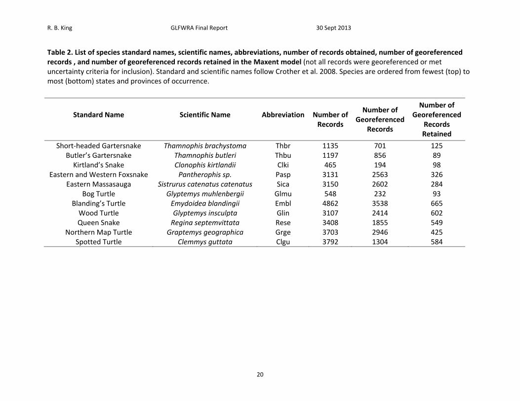
Table 2. List of species standard names, scientific names, abbreviations, number of records obtained, number of georeferenced records , and number of georeferenced records retained in the Maxent model (not all records were georeferenced or met uncertainty criteria for inclusion). Standard and scientific names follow Crother et al. 2008. Species are ordered from fewest (top) to most (bottom) states and provinces of occurrence.
Standard Name Scientific Name Abbreviation Number of Records
Number of Georeferenced
Records
Number of Georeferenced
Records Retained
Short‐headed Gartersnake Thamnophis brachystoma Thbr 1135 701 125 Butler’s Gartersnake Thamnophis butleri Thbu 1197 856 89 Kirtland’s Snake Clonophis kirtlandii Clki 465 194 98
Eastern and Western Foxsnake Pantherophis sp. Pasp 3131 2563 326 Eastern Massasauga Sistrurus catenatus catenatus Sica 3150 2602 284
Bog Turtle Glyptemys muhlenbergii Glmu 548 232 93 Blanding’s Turtle Emydoidea blandingii Embl 4862 3538 665 Wood Turtle Glyptemys insculpta Glin 3107 2414 602 Queen Snake Regina septemvittata Rese 3408 1855 549
Northern Map Turtle Graptemys geographica Grge 3703 2946 425 Spotted Turtle Clemmys guttata Clgu 3792 1304 584
R. B. King GLFWRA Final Report 30 Sept 2013
21
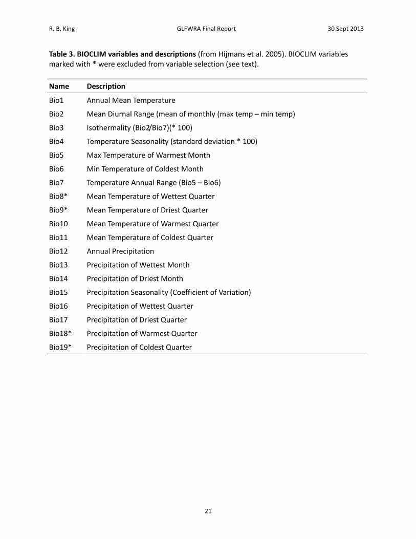
Table 3. BIOCLIM variables and descriptions (from Hijmans et al. 2005). BIOCLIM variables marked with * were excluded from variable selection (see text).
Name Description
Bio1 Annual Mean Temperature
Bio2 Mean Diurnal Range (mean of monthly (max temp – min temp)
Bio3 Isothermality (Bio2/Bio7)(* 100)
Bio4 Temperature Seasonality (standard deviation * 100)
Bio5 Max Temperature of Warmest Month
Bio6 Min Temperature of Coldest Month
Bio7 Temperature Annual Range (Bio5 – Bio6)
Bio8* Mean Temperature of Wettest Quarter
Bio9* Mean Temperature of Driest Quarter
Bio10 Mean Temperature of Warmest Quarter
Bio11 Mean Temperature of Coldest Quarter
Bio12 Annual Precipitation
Bio13 Precipitation of Wettest Month
Bio14 Precipitation of Driest Month
Bio15 Precipitation Seasonality (Coefficient of Variation)
Bio16 Precipitation of Wettest Quarter
Bio17 Precipitation of Driest Quarter
Bio18* Precipitation of Warmest Quarter
Bio19* Precipitation of Coldest Quarter
R. B. King GLFWRA Final Report 30 Sept 2013
22
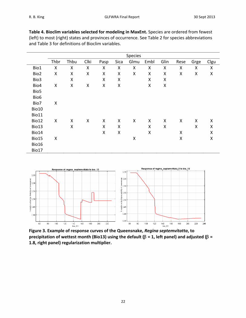
Table 4. Bioclim variables selected for modeling in MaxEnt. Species are ordered from fewest (left) to most (right) states and provinces of occurrence. See Table 2 for species abbreviations and Table 3 for definitions of Bioclim variables.
Species
Thbr Thbu Clki Pasp Sica Glmu Embl Glin Rese Grge Clgu
Bio1 X X X X X X X X X X X Bio2 X X X X X X X X X X X Bio3 X X X X X Bio4 X X X X X X X Bio5 Bio6 Bio7 X Bio10 Bio11 Bio12 X X X X X X X X X X X Bio13 X X X X X X X Bio14 X X X X X Bio15 X X X X Bio16 Bio17
Figure 3. Example of response curves of the Queensnake, Regina septemvitatta, to
precipitation of wettest month (Bio13) using the default ( = 1, left panel) and adjusted ( = 1.8, right panel) regularization multiplier.
R. B. King GLFWRA Final Report 30 Sept 2013
23
Results A total of 28,498 records were acquired for all species combined (Table 2). The number of records by species ranged from 465 for Clonophis kirtlandii to 4,862 for Emydoidea blandingii. The total number of georeferenced records, either from records that had latitude and longitude or from records that could georeferenced using GeoLocate, was 19,205. The total number of georeferenced records retained after applying the spatial filtering method was 3,840. The number of records retained by species ranged from 89 for Thamnophis butleri to 665 for Emydoidea blandingii (Table 2). Current Climate (1950 – 2000) Model. – Among the 11 species analyzed, four to seven BIOCLIM variables were retained for analysis following variable selection (Table 4). Annual mean temperature (Bio1), mean diurnal temperature range (Bio2), and annual precipitation (Bio12) were the only BIOCLIM variables included in all of the models (Table 4). Isothermality (Bio3) was included in the models for Emydoidea blandingii, Glyptemys insculpta, Pantherophis sp., Sistrurus catenatus catenatus, and Thamnophis butleri. Temperature seasonality (Bio4) was included in the models for Clonophis kirtlandii, Emydoidea blandingii, Glyptemys insculpta, Pantherophis sp., Sistrurus catenatus catenatus, Thamnophis brachystoma, and Thamnophis butleri. Temperature annual range (Bio7) was only included in the model for Thamnophis brachystoma. Precipitation of the wettest month (Bio13) was included in the models for Clemmys guttata, Emydoidea blandingii, Glyptemys insculpta, Graptemys geographica, Pantherophis species, Sistrurus catenatus catenatus, and Thamnophis butleri. Precipitation of the driest month (Bio 14) was included in the models for Clemmys guttata, Emydoidea blandingii, Pantherophis species, Regina septemvittata, and Sistrurus catenatus catenatus. Precipitation seasonality (Bio15) was included in the models for Clemmys guttata, Clemmys muhlenbergii, Sistrurus catenatus catenatus, and Thamnophis brachystoma. Maximum temperature of the warmest month (Bio5), minimum temperature of the warmest month (Bio6), mean temperature of the warmest quarter (Bio10), mean temperature of the coldest quarter (Bio11), precipitation of the wettest quarter (Bio16), and precipitation of the driest quarter (Bio17) were never included in any of the models. Training values for area under the receiver curve (AUC) for the models ranged from 0.74 to 0.95 and testing AUC values for the models ranged from 0.73 to 0.94 (Table 5). Models for species with smaller distributions typically had higher AUC values (Pearson correlation between area within 250 km buffers and testing AUC = ‐0.805, N = 11, P = 0.003). For example, Sistrurus catenatus catenatus and Graptemys geographica, two species with particularly large distributions, had testing AUC values of 0.73 and 0.77 respectively. Thamnophis brachystoma, an exemplar of a species with a small distribution, had the highest testing AUC of 0.94. Models predicted current distributions of target species well (Figures 4‐14; figures are ordered from showing the least to greatest projected decrease in climatic suitability as measured by the proportion of locations falling above the SSS threshold in 2050). Under current climate (1950 – 2000) conditions, greater than 70% of known localities for each species fell within the maximum sum of sensitivity and specificity (SSS) threshold (Table 6). Furthermore, areas of high suitability (above the SSS threshold) were largely restricted to within the 250 km buffer around
R. B. King GLFWRA Final Report 30 Sept 2013
24
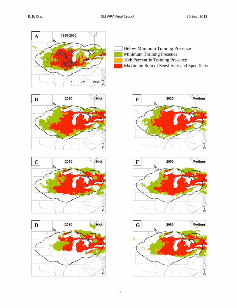
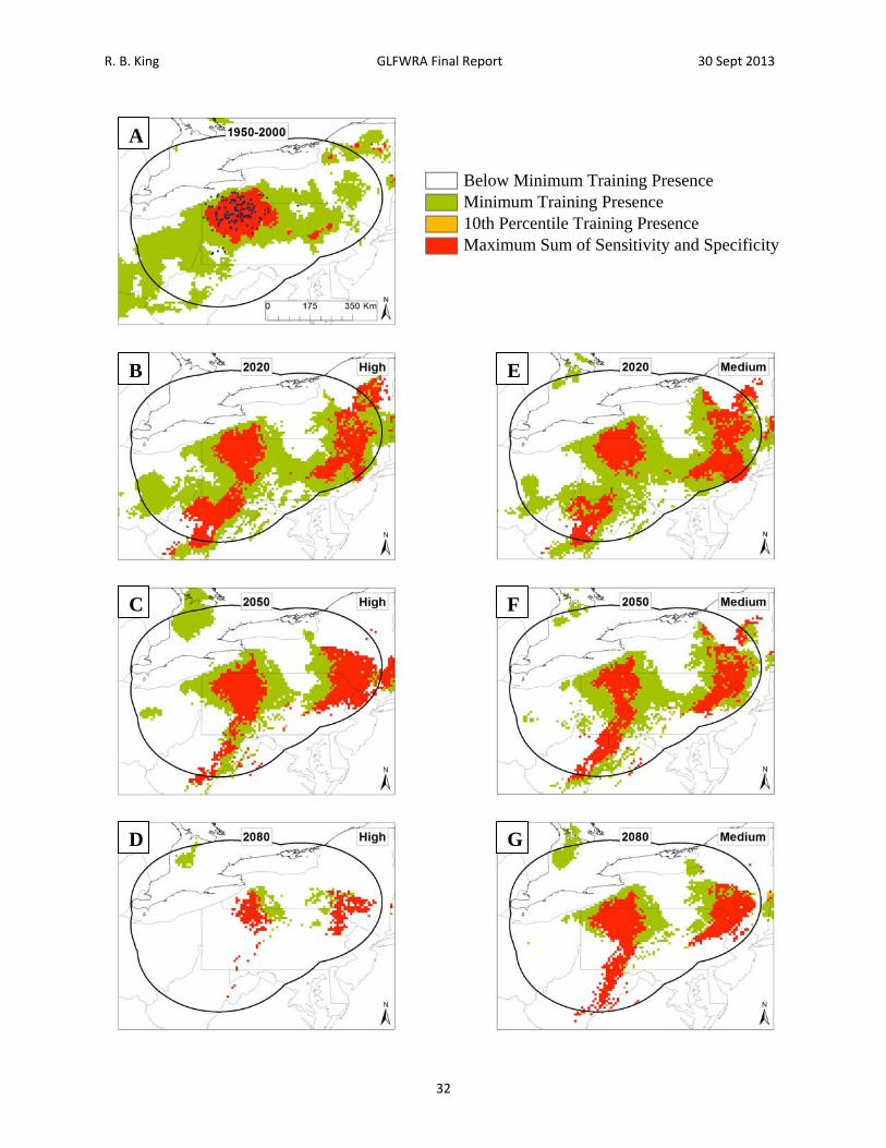
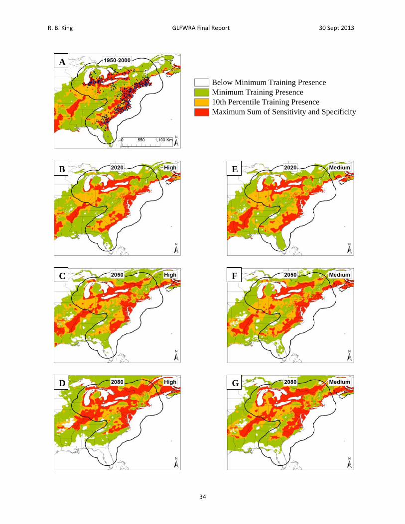
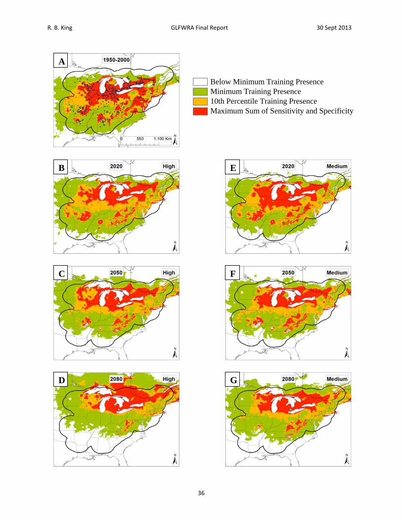
known occurrences (Figure 4‐14). Clemmys guttata was an exception in this regard with a significant area above the SSS threshold occurring southwest of the buffer area (Figure 7). Based on percent contribution and on permutation importance, annual mean temperature (Bio1) was a major contributor to models for all turtle species (Table 5). Other important contributors included mean diurnal range (Bio2) for Clemmys guttata, temperature seasonality (Bio4) for Glyptemys insculpta, annual precipitation (Bio12) for Emydoidea blandingii, precipitation of the wettest month (Bio13) for Graptemys geographica, and precipitation seasonality (Bio15) for Glyptemys muhlenbergii, (Table 5). For snake species, no single variable emerged as consistently being the highest contributor, although annual mean temperature frequently contributed more than 20% to the models. Other important contributors included mean diurnal range (Bio2) in Clonophis kirtlandii and Thamnophis butleri; isothermality (Bio3) in Pantherophis sp.; temperature seasonality (Bio4) in Clonophis kirtlandii, Pantherophis sp., Sistrurus catenatus catenatus, and Thamnophis butleri; annual precipitation (Bio12) in Pantherophis sp., Sistrurus catenatus catenatus, Thamnophis brachystoma, and Thamnophis butleri; and precipitation seasonality (Bio15) in Regina septemvittata and Thamnophis butleri (Table 5). Permutation importance was typically similar to the percent contribution, although relative contributions differed in some species (e.g., Glyptemys insculpta, Pantherophis sp., Sistrurus catenatus catenatus; Table 6). For mean annual temperature (Bio1), all species except Thamnophis brachystoma displayed a generally unimodal convex response curve (Figure 15, Table 6); areas of high climatic suitability had intermediate mean annual temperatures. Response curves for other Bioclim variables differed in shape among species (Table 6). Future Climate Projections. – Most projections indicated loss of climatic suitability originating along the southern and western edges of the species’ distributions (Figures 4‐14). However, species differed in the patterns of contraction and fragmentation of highly climatically suitable areas (area exceeding the maximum sum of sensitivity and specificity threshold). Clonophis kirtlandii, Regina septemvittata, and Sistrurus catenatus catenatus have single contiguous areas of high suitability under current conditions that are projected to contract and fragment into multiple smaller areas (Figures 10, 11 and 13). Emydoidea blandingii, Pantherophis sp., and Thamnophis brachystoma have single contiguous areas of high suitability under current conditions that are projected to shrink and shift to the northeast (Figures 6, 6, and 9). Clemmys guttata and Thamnophis butleri have multiple areas of high suitability under current conditions that are projected to merge over time (Figures 4 and 7). Glyptemys insculpta, Glyptemys muhlenbergii, and Graptemys geographica have multiple areas of high suitability that are projected to shrink or be lost (Figures 8, 12, and 14). To quantify change in climatic suitability, the known species localities used to generate the models were compared to against the threshold values, calculating the percentage of localities that fell within the threshold for each time period. Of the SRES scenarios, the high emission (A2a) scenario resulted in loss of climatic suitability for a greater number of known localities than the medium emission (B2a) scenario (Table 7, 16). This difference between scenarios was evident in all future projections for Clonophis kirtlandii, Glyptemys insculpta, Glyptemys muhlenbergii, and Sisturus catenatus catenatus but only in the 2080 projection for Emydoidia
R. B. King GLFWRA Final Report 30 Sept 2013
25
blandingii, Graptemys geographica, Panterhophis sp., Regina septemvittata, and Thamnophis brachystoma. Differences between scenarios were negligible for Clemmys guttata and Thamnophis butleri. In an effort to identify sets of species that might be similarly affected by climate change, species were classified according to the proportion of known localities falling above the maximum sum of sensitivity and specificity (SSS) threshold under the A2a scenario in 2050 (Table 6). By this criterion, Thamnohis butleri, Pantherophis species, and Thamnophis brachystoma were projected to have greater than 75% of known localities remain climatically suitable; Clemmys guttata and Graptemys geogrpahica were projected to have 50‐75% of known localities remain climatically suitable; Emydoidea blandingii, Regina septemvittata, and Sistrurus catenatus catenatus were projected to have 25‐50% of known localities remain climatically suitable; and Clonophis kirtlandii, Glyptemys insculpta, and Glyptemys muhlenbergii were projected to have less than 25% of known localities remain climatically suitable. Examining the same criteria in the year 2080, Thamnophis butleri falls to 50‐75%, Pantherophis species and Thamnophis brachystoma fall to 25‐50%, and Emydoidea blandingii, Regina septemvittata, and Sistrurus catenatus catenatus fall to below 25% of known localities remaining climatically suitable. A second method of quantifying the change in climatic suitability compared the size of the area satisfying a given threshold value to the size of the geographic background (Table 8, Figure 17). This approach allows for increases in the size of the area deemed climatically suitable. By this method, differences between the A2a and B2a scenarios were generally negligible before 2080 (but see Thamnophis butleri; Figure 4). Areas of climatic suitability were projected to increase for Clemmys guttata, remain constant for Graptemys geographica, first increase and then decrease for Pantherophis sp., Thamnophis brachystoma, and Thamnophis butleri, and steadily decrease for all other species (Table 8, Figure 17). Neither quantitative measure of change in climatic suitability was correlated with area curreltny occupied by species. Proportion of points above the SSS threshold in 2050 under the A2a scenario was uncorrelated with the size of the geographic background (area with 250 km buffers; Pearson’s correlation = ‐0.152, N = 11, P = 0.689). Similarly, the proportion of the area above the SSS threshold in 2050 under the A2a scenario was uncorrelated with the size of the geographic background (area with 250 km buffers; Pearson’s correlation = 0.139, N = 11, P = 0.689).
R. B. King GLFWRA Final Report 30 Sept 2013
26
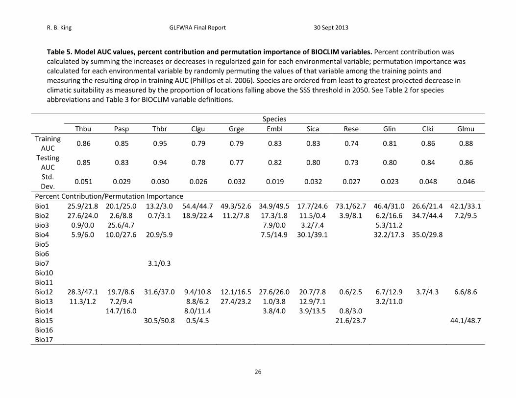
Table 5. Model AUC values, percent contribution and permutation importance of BIOCLIM variables. Percent contribution was calculated by summing the increases or decreases in regularized gain for each environmental variable; permutation importance was calculated for each environmental variable by randomly permuting the values of that variable among the training points and measuring the resulting drop in training AUC (Phillips et al. 2006). Species are ordered from least to greatest projected decrease in climatic suitability as measured by the proportion of locations falling above the SSS threshold in 2050. See Table 2 for species abbreviations and Table 3 for BIOCLIM variable definitions.
Species
Thbu Pasp Thbr Clgu Grge Embl Sica Rese Glin Clki Glmu
Training AUC
0.86 0.85 0.95 0.79 0.79 0.83 0.83 0.74 0.81 0.86 0.88
Testing AUC
0.85 0.83 0.94 0.78 0.77 0.82 0.80 0.73 0.80 0.84 0.86
Std. Dev.
0.051 0.029 0.030 0.026 0.032 0.019 0.032 0.027 0.023 0.048 0.046
Percent Contribution/Permutation Importance
Bio1 25.9/21.8 20.1/25.0 13.2/3.0 54.4/44.7 49.3/52.6 34.9/49.5 17.7/24.6 73.1/62.7 46.4/31.0 26.6/21.4 42.1/33.1 Bio2 27.6/24.0 2.6/8.8 0.7/3.1 18.9/22.4 11.2/7.8 17.3/1.8 11.5/0.4 3.9/8.1 6.2/16.6 34.7/44.4 7.2/9.5 Bio3 0.9/0.0 25.6/4.7 7.9/0.0 3.2/7.4 5.3/11.2 Bio4 5.9/6.0 10.0/27.6 20.9/5.9 7.5/14.9 30.1/39.1 32.2/17.3 35.0/29.8 Bio5 Bio6 Bio7 3.1/0.3 Bio10 Bio11 Bio12 28.3/47.1 19.7/8.6 31.6/37.0 9.4/10.8 12.1/16.5 27.6/26.0 20.7/7.8 0.6/2.5 6.7/12.9 3.7/4.3 6.6/8.6 Bio13 11.3/1.2 7.2/9.4 8.8/6.2 27.4/23.2 1.0/3.8 12.9/7.1 3.2/11.0 Bio14 14.7/16.0 8.0/11.4 3.8/4.0 3.9/13.5 0.8/3.0 Bio15 30.5/50.8 0.5/4.5 21.6/23.7 44.1/48.7 Bio16 Bio17
R. B. King GLFWRA Final Report 30 Sept 2013
27
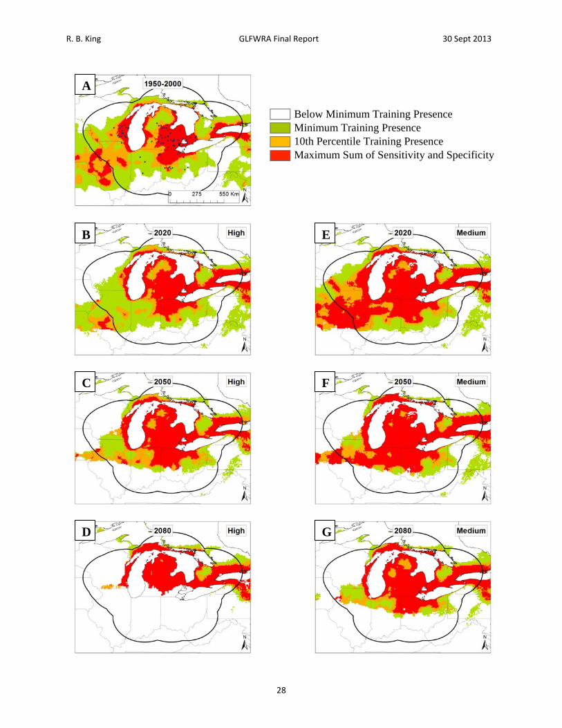
Figure 4. Current and future projections of climate suitability for Thamnophis butleri. Projections of climate suitability for Thamnophis butleri under current conditions (A) 1950‐2000, future conditions under the SRES A2a high emissions scenario (denoted ‘high’) for (B) 2020 (C) 2050 (D) 2080, and future conditions under the SRES B2a medium emissions scenario (denoted ‘medium’) scenario for (E) 2020 (F) 2050 (G) 2080. In each panel, areas falling above the minimum training presence threshold are green, areas falling above the tenth percentile threshold are gold, and areas falling above the maximum sum of sensitivity and specificity threshold are red. Presence records used in MaxEnt models are show as black dots in panel A. Locations have been ‘jittered’ by 0.1‐0.3 degrees (ca. 10‐35 km) to obscure the location of sensitive populations. The solid black line represents a 250 km buffer around presence records.
R. B. King GLFWRA Final Report 30 Sept 2013
28
Below Minimum Training Presence Minimum Training Presence 10th Percentile Training Presence Maximum Sum of Sensitivity and Specificity
A
B
C
D
E
F
G

R. B. King GLFWRA Final Report 30 Sept 2013
29
Figure 5. Current and future projections of climate suitability for Pantherophis sp. Projections of climate suitability for Pantherophis species under current conditions (A) 1950‐2000, future conditions under the SRES A2a high emissions scenario (denoted ‘high’) for (B) 2020 (C) 2050 (D) 2080, and future conditions under the SRES B2a medium emissions scenario (denoted ‘medium’) scenario for (E) 2020 (F) 2050 (G) 2080. In each panel, areas falling above the minimum training presence threshold are green, areas falling above the tenth percentile threshold are gold, and areas falling above the maximum sum of sensitivity and specificity threshold are red. Presence records used in MaxEnt models are show as black dots in panel A. Locations have been ‘jittered’ by 0.1‐0.3 degrees (ca. 10‐35 km) to obscure the location of sensitive populations. The solid black line represents a 250 km buffer around presence records.
R. B. King GLFWRA Final Report 30 Sept 2013
30
Below Minimum Training Presence Minimum Training Presence 10th Percentile Training Presence Maximum Sum of Sensitivity and Specificity
A
B
C
D
E
F
G
R. B. King GLFWRA Final Report 30 Sept 2013
31
Figure 6. Current and future projections of climate suitability for Thamnophis brachystoma. Projections of climate suitability for Thamnophis brachystoma under current conditions (A) 1950‐2000, future conditions under the SRES A2a high emissions scenario (denoted ‘high’) for (B) 2020 (C) 2050 (D) 2080, and future conditions under the SRES B2a medium emissions scenario (denoted ‘medium’) scenario for (E) 2020 (F) 2050 (G) 2080. In each panel, areas falling above the minimum training presence threshold are green, areas falling above the tenth percentile threshold are gold, and areas falling above the maximum sum of sensitivity and specificity threshold are red. Presence records used in MaxEnt models are show as black dots in panel A. Locations have been ‘jittered’ by 0.1‐0.3 degrees (ca. 10‐35 km) to obscure the location of sensitive populations. The solid black line represents a 250 km buffer around presence records.
R. B. King GLFWRA Final Report 30 Sept 2013
32
Below Minimum Training Presence Minimum Training Presence 10th Percentile Training Presence Maximum Sum of Sensitivity and Specificity
A
B
C
D
E
F
G
R. B. King GLFWRA Final Report 30 Sept 2013
33
Figure 7. Current and future projections of climate suitability for Clemmys guttata. Projections of climate suitability for Clemmys guttata under current conditions (A) 1950‐2000, future conditions under the SRES A2a high emissions scenario (denoted ‘high’) for (B) 2020 (C) 2050 (D) 2080, and future conditions under the SRES B2a medium emissions scenario (denoted ‘medium’) scenario for (E) 2020 (F) 2050 (G) 2080. In each panel, areas falling above the minimum training presence threshold are green, areas falling above the tenth percentile threshold are gold, and areas falling above the maximum sum of sensitivity and specificity threshold are red. Presence records used in MaxEnt models are show as black dots in panel A. Locations have been ‘jittered’ by 0.1‐0.3 degrees (ca. 10‐35 km) to obscure the location of sensitive populations. The solid black line represents a 250 km buffer around presence records.
R. B. King GLFWRA Final Report 30 Sept 2013
34
Below Minimum Training Presence Minimum Training Presence 10th Percentile Training Presence Maximum Sum of Sensitivity and Specificity
A
B
C
D
E
F
G
R. B. King GLFWRA Final Report 30 Sept 2013
35
Figure 8. Current and future projections of climate suitability for Graptemys geographica. Projections of climate suitability for Graptemys geographica under current conditions (A) 1950‐2000, future conditions under the SRES A2a high emissions scenario (denoted ‘high’) for (B) 2020 (C) 2050 (D) 2080, and future conditions under the SRES B2a medium emissions scenario (denoted ‘medium’) scenario for (E) 2020 (F) 2050 (G) 2080. In each panel, areas falling above the minimum training presence threshold are green, areas falling above the tenth percentile threshold are gold, and areas falling above the maximum sum of sensitivity and specificity threshold are red. Presence records used in MaxEnt models are show as black dots in panel A. Locations have been ‘jittered’ by 0.1‐0.3 degrees (ca. 10‐35 km) to obscure the location of sensitive populations. The solid black line represents a 250 km buffer around presence records.
R. B. King GLFWRA Final Report 30 Sept 2013
36
Below Minimum Training Presence Minimum Training Presence 10th Percentile Training Presence Maximum Sum of Sensitivity and Specificity
A
B
C
D
E
F
G
R. B. King GLFWRA Final Report 30 Sept 2013
37
Figure 9. Current and future projections of climate suitability for Emydoidea blandingii. Projections of climate suitability for Emydoidea blandingii under current conditions (A) 1950‐2000, future conditions under the SRES A2a high emissions scenario (denoted ‘high’) for (B) 2020 (C) 2050 (D) 2080, and future conditions under the SRES B2a medium emissions scenario (denoted ‘medium’) scenario for (E) 2020 (F) 2050 (G) 2080. In each panel, areas falling above the minimum training presence threshold are green, areas falling above the tenth percentile threshold are gold, and areas falling above the maximum sum of sensitivity and specificity threshold are red. Presence records used in MaxEnt models are show as black dots in panel A. Locations have been ‘jittered’ by 0.1‐0.3 degrees (ca. 10‐35 km) to obscure the location of sensitive populations. The solid black line represents a 250 km buffer around presence records.
R. B. King GLFWRA Final Report 30 Sept 2013
38
Below Minimum Training Presence Minimum Training Presence 10th Percentile Training Presence Maximum Sum of Sensitivity and Specificity
A
B
C
D
E
F
G
R. B. King GLFWRA Final Report 30 Sept 2013
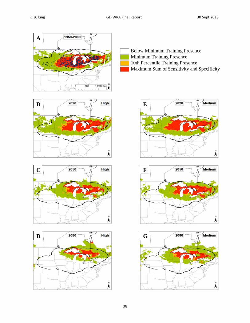
39
Figure 10. Current and future projections of climate suitability for Sistrurus catenatus catenatus. Projections of climate suitability for Sistrurus catenatus catenatus under current conditions (A) 1950‐2000, future conditions under the SRES A2a high emissions scenario (denoted ‘high’) for (B) 2020 (C) 2050 (D) 2080, and future conditions under the SRES B2a medium emissions scenario (denoted ‘medium’) scenario for (E) 2020 (F) 2050 (G) 2080. In each panel, areas falling above the minimum training presence threshold are green, areas falling above the tenth percentile threshold are gold, and areas falling above the maximum sum of sensitivity and specificity threshold are red. Presence records used in MaxEnt models are show as black dots in panel A. Locations have been ‘jittered’ by 0.1‐0.3 degrees (ca. 10‐35 km) to obscure the location of sensitive populations. The solid black line represents a 250 km buffer around presence records.
R. B. King GLFWRA Final Report 30 Sept 2013
40
Below Minimum Training Presence Minimum Training Presence 10th Percentile Training Presence Maximum Sum of Sensitivity and Specificity
A
B
C
D
E
F
G

R. B. King GLFWRA Final Report 30 Sept 2013
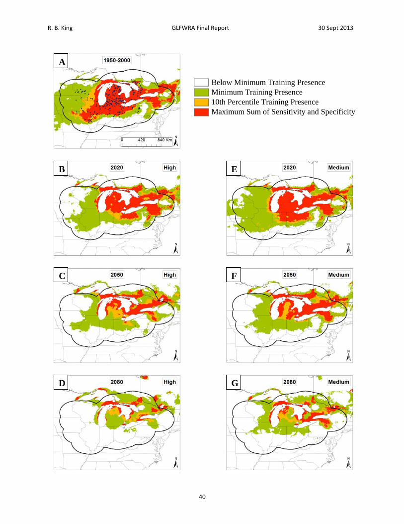
41
Figure 11. Current and future projections of climate suitability for Regina septemvittata. Projections of climate suitability for Regina septemvittata under current conditions (A) 1950‐2000, future conditions under the SRES A2a high emissions scenario (denoted ‘high’) for (B) 2020 (C) 2050 (D) 2080, and future conditions under the SRES B2a medium emissions scenario (denoted ‘medium’) scenario for (E) 2020 (F) 2050 (G) 2080. In each panel, areas falling above the minimum training presence threshold are green, areas falling above the tenth percentile threshold are gold, and areas falling above the maximum sum of sensitivity and specificity threshold are red. Presence records used in MaxEnt models are show as black dots in panel A. Locations have been ‘jittered’ by 0.1‐0.3 degrees (ca. 10‐35 km) to obscure the location of sensitive populations. The solid black line represents a 250 km buffer around presence records.
R. B. King GLFWRA Final Report 30 Sept 2013
42
Below Minimum Training Presence Minimum Training Presence 10th Percentile Training Presence Maximum Sum of Sensitivity and Specificity
A
B
C
D
E
F
G

R. B. King GLFWRA Final Report 30 Sept 2013
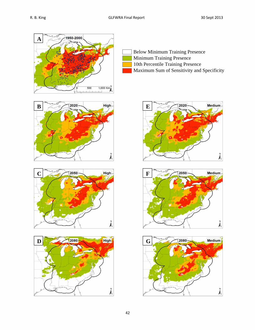
43
Figure 12. Current and future projections of climate suitability for Glyptemys insculpta. Projections of climate suitability for Glyptemys insculpta under current conditions (A) 1950‐2000, future conditions under the SRES A2a high emissions scenario (denoted ‘high’) for (B) 2020 (C) 2050 (D) 2080, and future conditions under the SRES B2a medium emissions scenario (denoted ‘medium’) scenario for (E) 2020 (F) 2050 (G) 2080. In each panel, areas falling above the minimum training presence threshold are green, areas falling above the tenth percentile threshold are gold, and areas falling above the maximum sum of sensitivity and specificity threshold are red. Presence records used in MaxEnt models are show as black dots in panel A. Locations have been ‘jittered’ by 0.1‐0.3 degrees (ca. 10‐35 km) to obscure the location of sensitive populations. The solid black line represents a 250 km buffer around presence records.
R. B. King GLFWRA Final Report 30 Sept 2013
44
Below Minimum Training Presence Minimum Training Presence 10th Percentile Training Presence Maximum Sum of Sensitivity and Specificity
A
B
C
D
E
F
G
R. B. King GLFWRA Final Report 30 Sept 2013
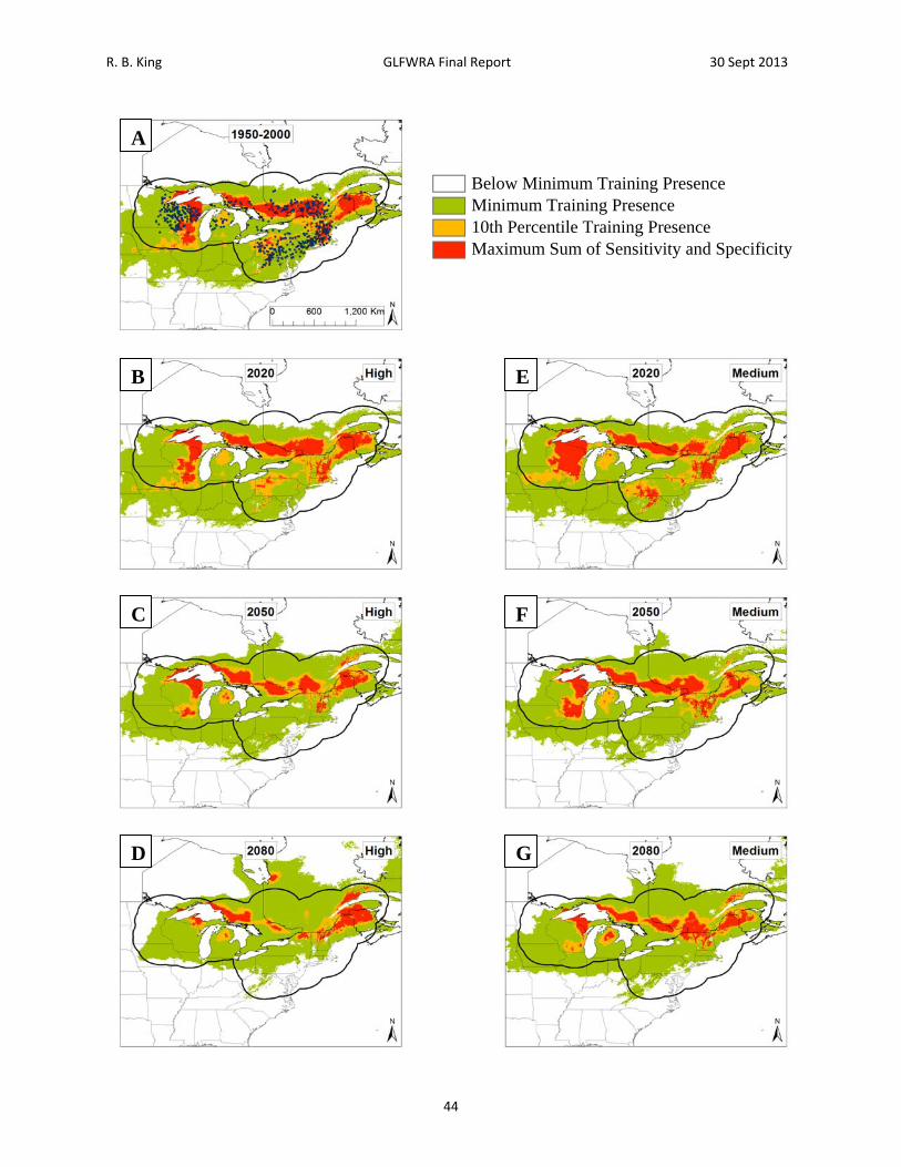
45
Figure 13. Current and future projections of climate suitability for Clonophis kirtlandii. Projections of climate suitability for Clonophis kirtlandii under current conditions (A) 1950‐2000, future conditions under the SRES A2a high emissions scenario (denoted ‘high’) for (B) 2020 (C) 2050 (D) 2080, and future conditions under the SRES B2a medium emissions scenario (denoted ‘medium’) scenario for (E) 2020 (F) 2050 (G) 2080. In each panel, areas falling above the minimum training presence threshold are green, areas falling above the tenth percentile threshold are gold, and areas falling above the maximum sum of sensitivity and specificity threshold are red. Presence records used in MaxEnt models are show as black dots in panel A. Locations have been ‘jittered’ by 0.1‐0.3 degrees (ca. 10‐35 km) to obscure the location of sensitive populations. The solid black line represents a 250 km buffer around presence records.
R. B. King GLFWRA Final Report 30 Sept 2013
46
Below Minimum Training Presence Minimum Training Presence 10th Percentile Training Presence Maximum Sum of Sensitivity and Specificity
A
B
C
D
E
F
G

R. B. King GLFWRA Final Report 30 Sept 2013
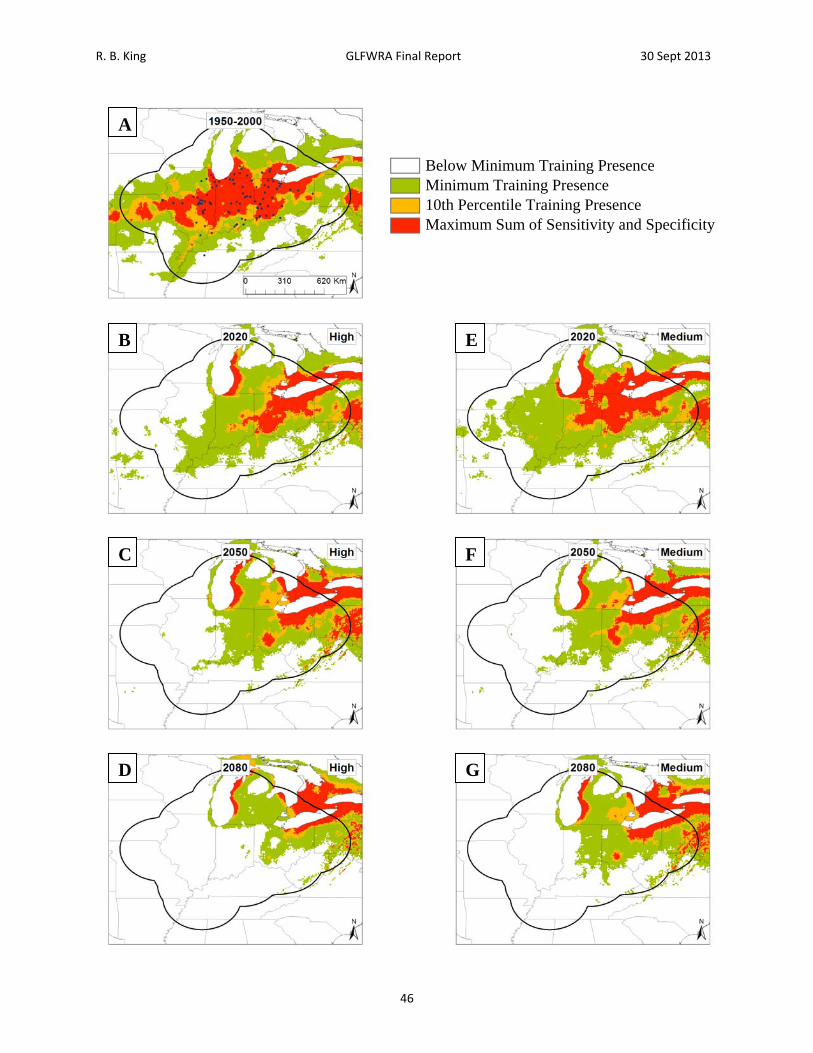
47
Figure 14. Current and future projections of climate suitability for Glyptemys muhlenbergii. Projections of climate suitability for Glyptemys muhlenbergii under current conditions (A) 1950‐2000, future conditions under the SRES A2a high emissions scenario (denoted ‘high’) for (B) 2020 (C) 2050 (D) 2080, and future conditions under the SRES B2a medium emissions scenario (denoted ‘medium’) scenario for (E) 2020 (F) 2050 (G) 2080. In each panel, areas falling above the minimum training presence threshold are green, areas falling above the tenth percentile threshold are gold, and areas falling above the maximum sum of sensitivity and specificity threshold are red. Presence records used in MaxEnt models are show as black dots in panel A. Locations have been ‘jittered’ by 0.1‐0.3 degrees (ca. 10‐35 km) to obscure the location of sensitive populations. The solid black line represents a 250 km buffer around presence records.
R. B. King GLFWRA Final Report 30 Sept 2013
48
Below Minimum Training Presence Minimum Training Presence 10th Percentile Training Presence Maximum Sum of Sensitivity and Specificity
A
B
C
D
E
F
G
R. B. King GLFWRA Final Report 30 Sept 2013
49
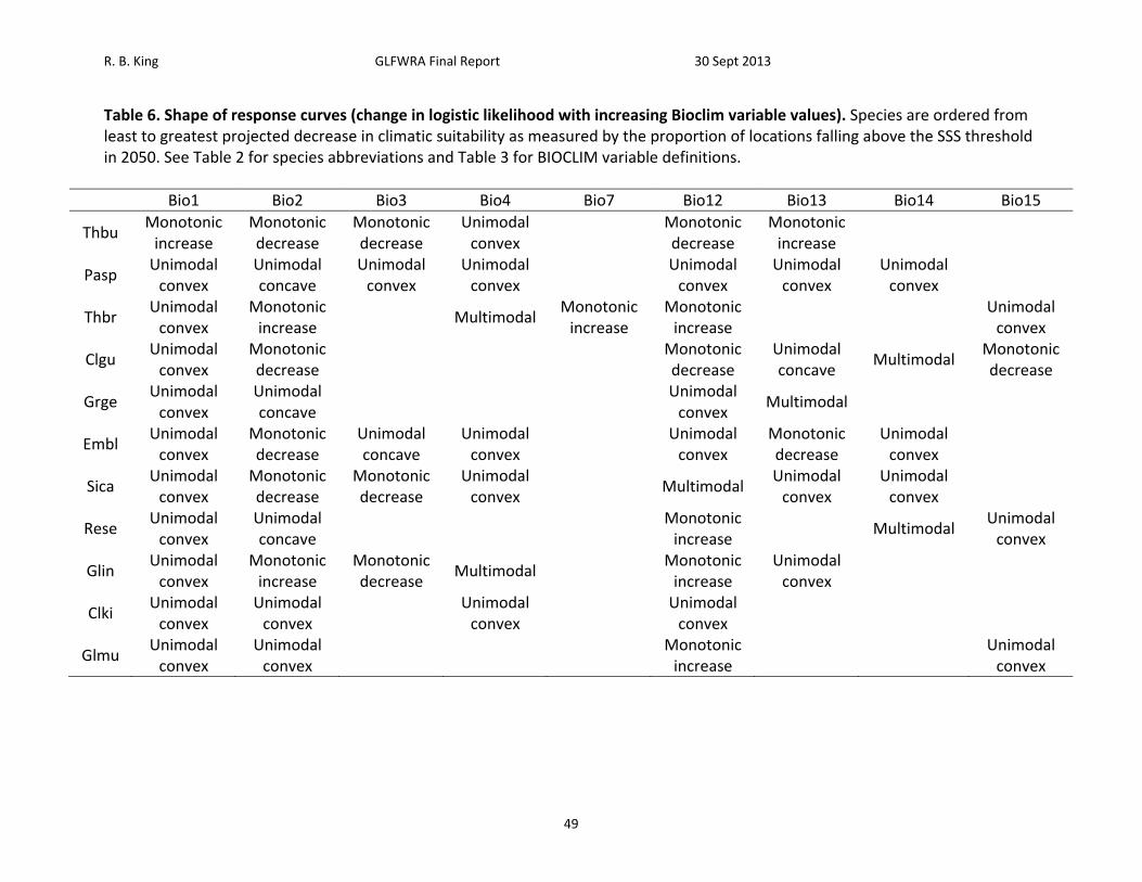
Table 6. Shape of response curves (change in logistic likelihood with increasing Bioclim variable values). Species are ordered from least to greatest projected decrease in climatic suitability as measured by the proportion of locations falling above the SSS threshold in 2050. See Table 2 for species abbreviations and Table 3 for BIOCLIM variable definitions.
Bio1 Bio2 Bio3 Bio4 Bio7 Bio12 Bio13 Bio14 Bio15
Thbu Monotonic increase
Monotonic decrease
Monotonic decrease
Unimodal convex
Monotonic decrease
Monotonic increase
Pasp Unimodal convex
Unimodal concave
Unimodal convex
Unimodal convex
Unimodal convex
Unimodal convex
Unimodal convex
Thbr Unimodal convex
Monotonic increase
Multimodal Monotonic increase
Monotonic increase
Unimodal convex
Clgu Unimodal convex
Monotonic decrease
Monotonic decrease
Unimodal concave
Multimodal Monotonic decrease
Grge Unimodal convex
Unimodal concave
Unimodal convex
Multimodal
Embl Unimodal convex
Monotonic decrease
Unimodal concave
Unimodal convex
Unimodal convex
Monotonic decrease
Unimodal convex
Sica Unimodal convex
Monotonic decrease
Monotonic decrease
Unimodal convex
Multimodal Unimodal convex
Unimodal convex
Rese Unimodal convex
Unimodal concave
Monotonic increase
Multimodal Unimodal convex
Glin Unimodal convex
Monotonic increase
Monotonic decrease
Multimodal Monotonic increase
Unimodal convex
Clki Unimodal convex
Unimodal convex
Unimodal convex
Unimodal convex
Glmu Unimodal convex
Unimodal convex
Monotonic increase
Unimodal convex
R. B. King GLFWRA Final Report 30 Sept 2013
50
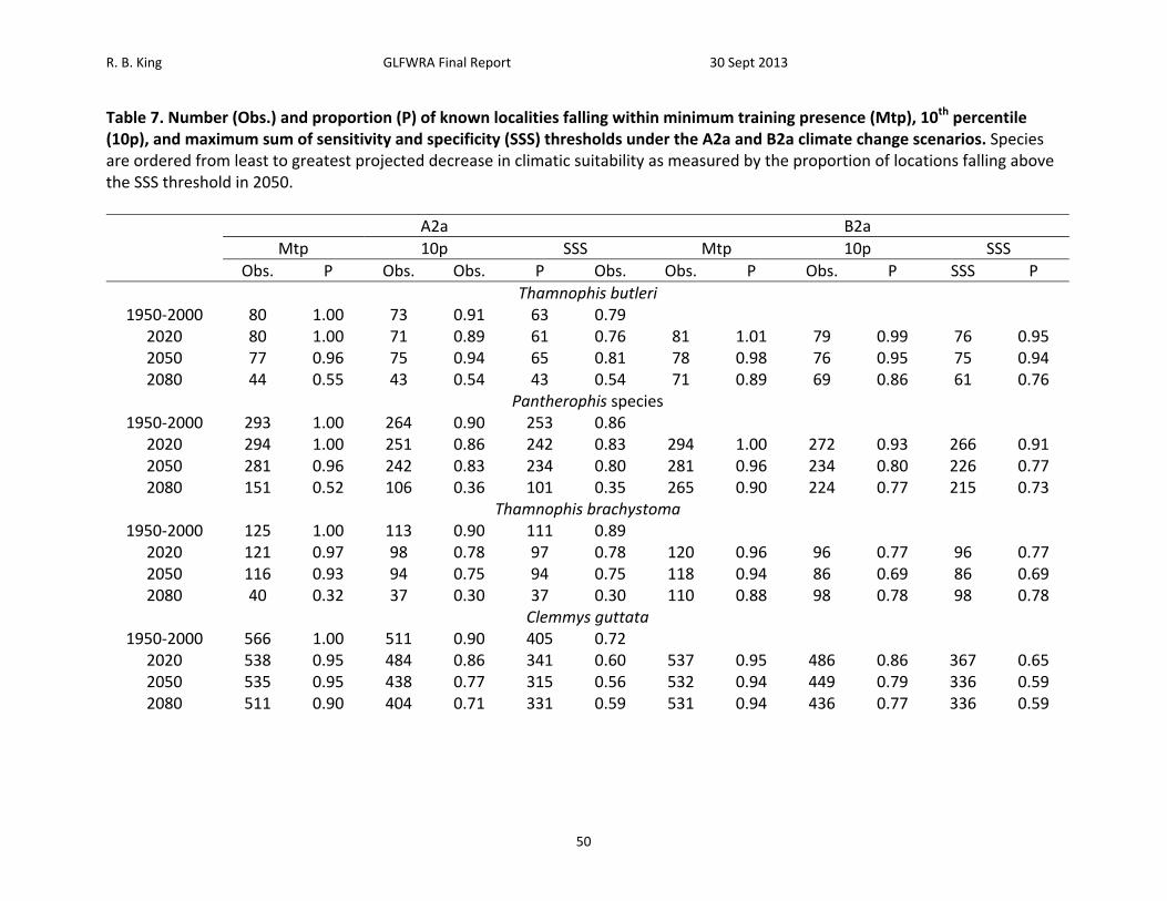
Table 7. Number (Obs.) and proportion (P) of known localities falling within minimum training presence (Mtp), 10th percentile (10p), and maximum sum of sensitivity and specificity (SSS) thresholds under the A2a and B2a climate change scenarios. Species are ordered from least to greatest projected decrease in climatic suitability as measured by the proportion of locations falling above the SSS threshold in 2050.
A2a B2a
Mtp 10p SSS Mtp 10p SSS
Obs. P Obs. Obs. P Obs. Obs. P Obs. P SSS P
Thamnophis butleri 1950‐2000 80 1.00 73 0.91 63 0.79
2020 80 1.00 71 0.89 61 0.76 81 1.01 79 0.99 76 0.95 2050 77 0.96 75 0.94 65 0.81 78 0.98 76 0.95 75 0.94 2080 44 0.55 43 0.54 43 0.54 71 0.89 69 0.86 61 0.76
Pantherophis species 1950‐2000 293 1.00 264 0.90 253 0.86
2020 294 1.00 251 0.86 242 0.83 294 1.00 272 0.93 266 0.91 2050 281 0.96 242 0.83 234 0.80 281 0.96 234 0.80 226 0.77 2080 151 0.52 106 0.36 101 0.35 265 0.90 224 0.77 215 0.73
Thamnophis brachystoma 1950‐2000 125 1.00 113 0.90 111 0.89
2020 121 0.97 98 0.78 97 0.78 120 0.96 96 0.77 96 0.77 2050 116 0.93 94 0.75 94 0.75 118 0.94 86 0.69 86 0.69 2080 40 0.32 37 0.30 37 0.30 110 0.88 98 0.78 98 0.78
Clemmys guttata 1950‐2000 566 1.00 511 0.90 405 0.72
2020 538 0.95 484 0.86 341 0.60 537 0.95 486 0.86 367 0.65 2050 535 0.95 438 0.77 315 0.56 532 0.94 449 0.79 336 0.59 2080 511 0.90 404 0.71 331 0.59 531 0.94 436 0.77 336 0.59
R. B. King GLFWRA Final Report 30 Sept 2013
51
A2a B2a
Mtp 10p SSS Mtp 10p SSS
Obs. P Obs. Obs. P Obs. Obs. P Obs. P SSS P
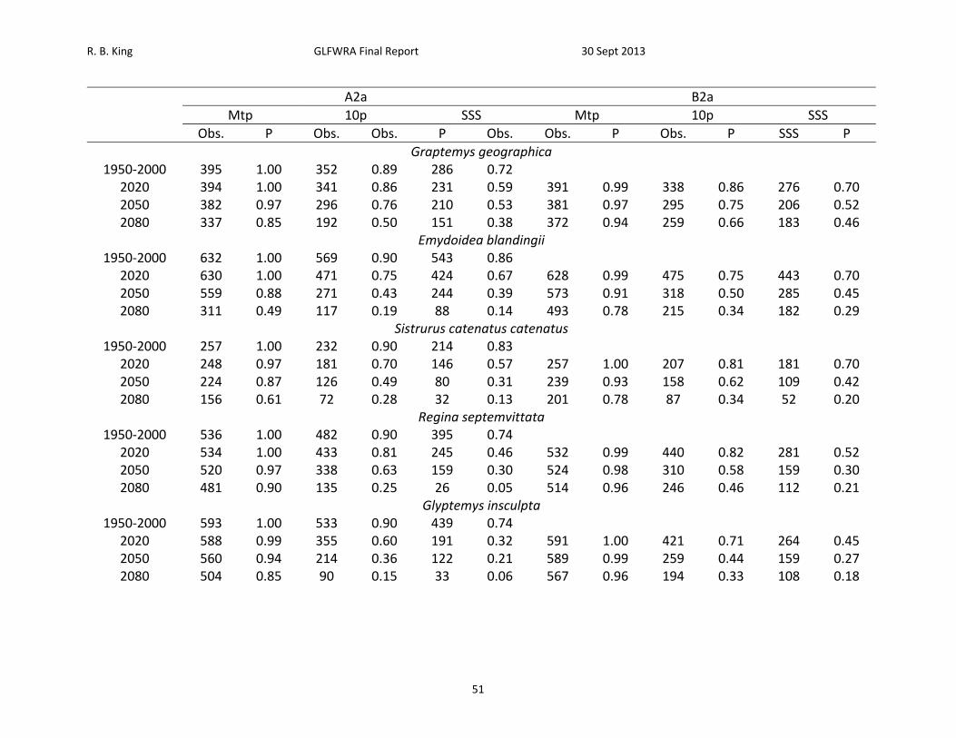
Graptemys geographica 1950‐2000 395 1.00 352 0.89 286 0.72
2020 394 1.00 341 0.86 231 0.59 391 0.99 338 0.86 276 0.70 2050 382 0.97 296 0.76 210 0.53 381 0.97 295 0.75 206 0.52 2080 337 0.85 192 0.50 151 0.38 372 0.94 259 0.66 183 0.46
Emydoidea blandingii 1950‐2000 632 1.00 569 0.90 543 0.86
2020 630 1.00 471 0.75 424 0.67 628 0.99 475 0.75 443 0.70 2050 559 0.88 271 0.43 244 0.39 573 0.91 318 0.50 285 0.45 2080 311 0.49 117 0.19 88 0.14 493 0.78 215 0.34 182 0.29
Sistrurus catenatus catenatus 1950‐2000 257 1.00 232 0.90 214 0.83
2020 248 0.97 181 0.70 146 0.57 257 1.00 207 0.81 181 0.70 2050 224 0.87 126 0.49 80 0.31 239 0.93 158 0.62 109 0.42 2080 156 0.61 72 0.28 32 0.13 201 0.78 87 0.34 52 0.20
Regina septemvittata 1950‐2000 536 1.00 482 0.90 395 0.74
2020 534 1.00 433 0.81 245 0.46 532 0.99 440 0.82 281 0.52 2050 520 0.97 338 0.63 159 0.30 524 0.98 310 0.58 159 0.30 2080 481 0.90 135 0.25 26 0.05 514 0.96 246 0.46 112 0.21
Glyptemys insculpta 1950‐2000 593 1.00 533 0.90 439 0.74
2020 588 0.99 355 0.60 191 0.32 591 1.00 421 0.71 264 0.45 2050 560 0.94 214 0.36 122 0.21 589 0.99 259 0.44 159 0.27 2080 504 0.85 90 0.15 33 0.06 567 0.96 194 0.33 108 0.18
R. B. King GLFWRA Final Report 30 Sept 2013
52
A2a B2a
Mtp 10p SSS Mtp 10p SSS
Obs. P Obs. Obs. P Obs. Obs. P Obs. P SSS P
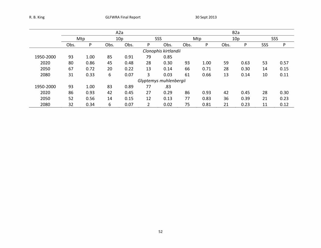
Clonophis kirtlandii 1950‐2000 93 1.00 85 0.91 79 0.85
2020 80 0.86 45 0.48 28 0.30 93 1.00 59 0.63 53 0.57 2050 67 0.72 20 0.22 13 0.14 66 0.71 28 0.30 14 0.15 2080 31 0.33 6 0.07 3 0.03 61 0.66 13 0.14 10 0.11
Glyptemys muhlenbergii 1950‐2000 93 1.00 83 0.89 77 .83
2020 86 0.93 42 0.45 27 0.29 86 0.93 42 0.45 28 0.30 2050 52 0.56 14 0.15 12 0.13 77 0.83 36 0.39 21 0.23 2080 32 0.34 6 0.07 2 0.02 75 0.81 21 0.23 11 0.12
R. B. King GLFWRA Final Report 30 Sept 2013
53
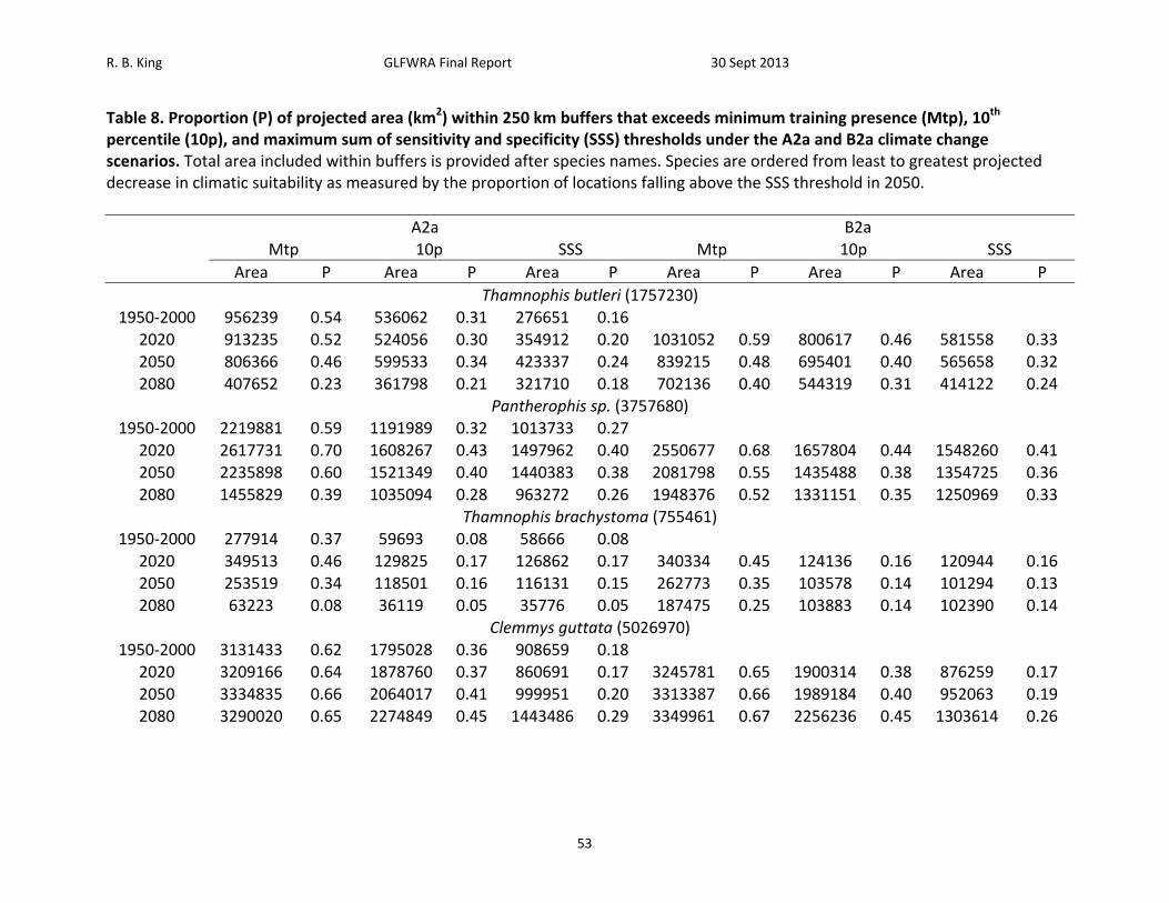
Table 8. Proportion (P) of projected area (km2) within 250 km buffers that exceeds minimum training presence (Mtp), 10th percentile (10p), and maximum sum of sensitivity and specificity (SSS) thresholds under the A2a and B2a climate change scenarios. Total area included within buffers is provided after species names. Species are ordered from least to greatest projected decrease in climatic suitability as measured by the proportion of locations falling above the SSS threshold in 2050.
A2a B2a Mtp 10p SSS Mtp 10p SSS
Area P Area P Area P Area P Area P Area P
Thamnophis butleri (1757230) 1950‐2000 956239 0.54 536062 0.31 276651 0.16
2020 913235 0.52 524056 0.30 354912 0.20 1031052 0.59 800617 0.46 581558 0.33 2050 806366 0.46 599533 0.34 423337 0.24 839215 0.48 695401 0.40 565658 0.32 2080 407652 0.23 361798 0.21 321710 0.18 702136 0.40 544319 0.31 414122 0.24
Pantherophis sp. (3757680) 1950‐2000 2219881 0.59 1191989 0.32 1013733 0.27
2020 2617731 0.70 1608267 0.43 1497962 0.40 2550677 0.68 1657804 0.44 1548260 0.41 2050 2235898 0.60 1521349 0.40 1440383 0.38 2081798 0.55 1435488 0.38 1354725 0.36 2080 1455829 0.39 1035094 0.28 963272 0.26 1948376 0.52 1331151 0.35 1250969 0.33
Thamnophis brachystoma (755461) 1950‐2000 277914 0.37 59693 0.08 58666 0.08
2020 349513 0.46 129825 0.17 126862 0.17 340334 0.45 124136 0.16 120944 0.16 2050 253519 0.34 118501 0.16 116131 0.15 262773 0.35 103578 0.14 101294 0.13 2080 63223 0.08 36119 0.05 35776 0.05 187475 0.25 103883 0.14 102390 0.14
Clemmys guttata (5026970) 1950‐2000 3131433 0.62 1795028 0.36 908659 0.18
2020 3209166 0.64 1878760 0.37 860691 0.17 3245781 0.65 1900314 0.38 876259 0.17 2050 3334835 0.66 2064017 0.41 999951 0.20 3313387 0.66 1989184 0.40 952063 0.19 2080 3290020 0.65 2274849 0.45 1443486 0.29 3349961 0.67 2256236 0.45 1303614 0.26
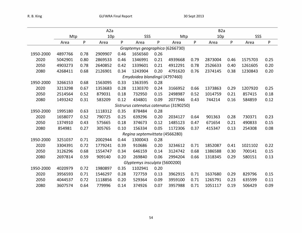
R. B. King GLFWRA Final Report 30 Sept 2013
54
A2a B2a Mtp 10p SSS Mtp 10p SSS
Area P Area P Area P Area P Area P Area P
Graptemys geographica (6266730) 1950‐2000 4897766 0.78 2909907 0.46 1656560 0.26
2020 5042901 0.80 2869533 0.46 1346991 0.21 4939668 0.79 2873004 0.46 1575703 0.25 2050 4903273 0.78 2640852 0.42 1339601 0.21 4912291 0.78 2526633 0.40 1261605 0.20 2080 4268411 0.68 2126901 0.34 1243904 0.20 4791620 0.76 2374145 0.38 1230843 0.20
Emydoidea blandingii (4797460) 1950‐2000 3266153 0.68 1563095 0.33 1363595 0.28
2020 3213298 0.67 1353683 0.28 1130370 0.24 3166952 0.66 1373863 0.29 1207920 0.25 2050 2514564 0.52 879031 0.18 732950 0.15 2498987 0.52 1014759 0.21 857415 0.18 2080 1493242 0.31 583209 0.12 434801 0.09 2077946 0.43 744214 0.16 584859 0.12
Sistrurus catenatus catenatus (3190250) 1950‐2000 1995180 0.63 1118312 0.35 878484 0.28
2020 1658077 0.52 790725 0.25 639296 0.20 2034127 0.64 901363 0.28 730371 0.23 2050 1374910 0.43 575665 0.18 374673 0.12 1485123 0.47 671654 0.21 490833 0.15 2080 854981 0.27 305765 0.10 156334 0.05 1172306 0.37 415347 0.13 254308 0.08
Regina septemvittata (4566280) 1950‐2000 3251037 0.71 2002944 0.44 1300043 0.28
2020 3304391 0.72 1779241 0.39 910686 0.20 3234612 0.71 1852087 0.41 1021102 0.22 2050 3126296 0.68 1554747 0.34 646159 0.14 3124742 0.68 1386588 0.30 700141 0.15 2080 2697814 0.59 909140 0.20 269840 0.06 2994204 0.66 1318345 0.29 580151 0.13
Glyptemys insculpta (5600200) 1950‐2000 4020979 0.72 1980897 0.35 1102941 0.20
2020 3956593 0.71 1546297 0.28 727759 0.13 3962915 0.71 1637680 0.29 829796 0.15 2050 4044537 0.72 1118856 0.20 529364 0.09 3959100 0.71 1265791 0.23 635599 0.11 2080 3607574 0.64 779996 0.14 374926 0.07 3957988 0.71 1051117 0.19 506429 0.09
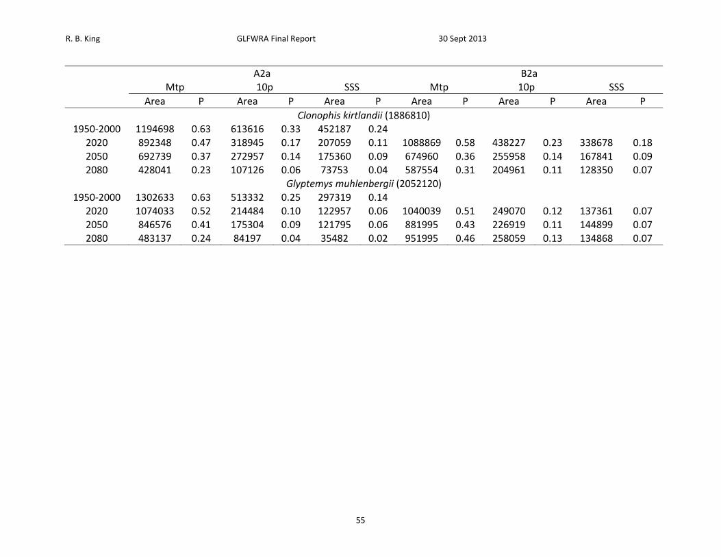
R. B. King GLFWRA Final Report 30 Sept 2013
55
A2a B2a Mtp 10p SSS Mtp 10p SSS
Area P Area P Area P Area P Area P Area P
Clonophis kirtlandii (1886810) 1950‐2000 1194698 0.63 613616 0.33 452187 0.24
2020 892348 0.47 318945 0.17 207059 0.11 1088869 0.58 438227 0.23 338678 0.18 2050 692739 0.37 272957 0.14 175360 0.09 674960 0.36 255958 0.14 167841 0.09 2080 428041 0.23 107126 0.06 73753 0.04 587554 0.31 204961 0.11 128350 0.07
Glyptemys muhlenbergii (2052120) 1950‐2000 1302633 0.63 513332 0.25 297319 0.14
2020 1074033 0.52 214484 0.10 122957 0.06 1040039 0.51 249070 0.12 137361 0.07 2050 846576 0.41 175304 0.09 121795 0.06 881995 0.43 226919 0.11 144899 0.07 2080 483137 0.24 84197 0.04 35482 0.02 951995 0.46 258059 0.13 134868 0.07
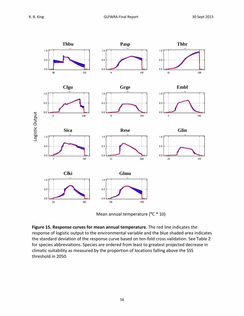
R. B. King GLFWRA Final Report 30 Sept 2013
56
Figure 15. Response curves for mean annual temperature. The red line indicates the response of logistic output to the environmental variable and the blue shaded area indicates the standard deviation of the response curve based on ten‐fold cross validation. See Table 2 for species abbreviations. Species are ordered from least to greatest projected decrease in climatic suitability as measured by the proportion of locations falling above the SSS threshold in 2050.
Clgu
Glmu Clki
Embl Grge
Glin
Pasp
Rese Sica
Thbr Thbu
Logistic Output
Mean annual temperature (⁰C * 10)
R. B. King GLFWRA Final Report 30 Sept 2013
57
Figure 16. Temporal change in area of climatic suitability based on the proportion of presence records that fall within areas delineated by MTP (green), 10P (gold), and SSS (red) threseholds under A2a (circles) and B2a (squares) scenarios. Current conditions (1950‐2000) are represented by points located at 1990. Species are ordered from least to greatest projected decrease in climatic suitability as measured by the proportion of locations falling above the SSS threshold in 2050. See Table 2 for species abbreviations.
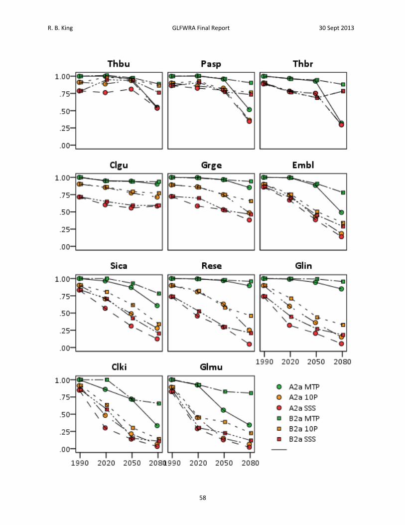
R. B. King GLFWRA Final Report 30 Sept 2013
58
R. B. King GLFWRA Final Report 30 Sept 2013
59
Figure 17. Temporal change in area of climatic suitability based on the proportion of background area (presence records with 250 km buffer) that falls within areas delineated by MTP (green), 10P (gold), and SSS (red) threseholds under A2a (circles) and B2a (squares) scenarios. Current conditions (1950‐2000) are represented by points located at 1990. Species are ordered from least to greatest projected decrease in climatic suitability as measured by the proportion of locations falling above the SSS threshold in 2050. See Table 2 for species abbreviations.
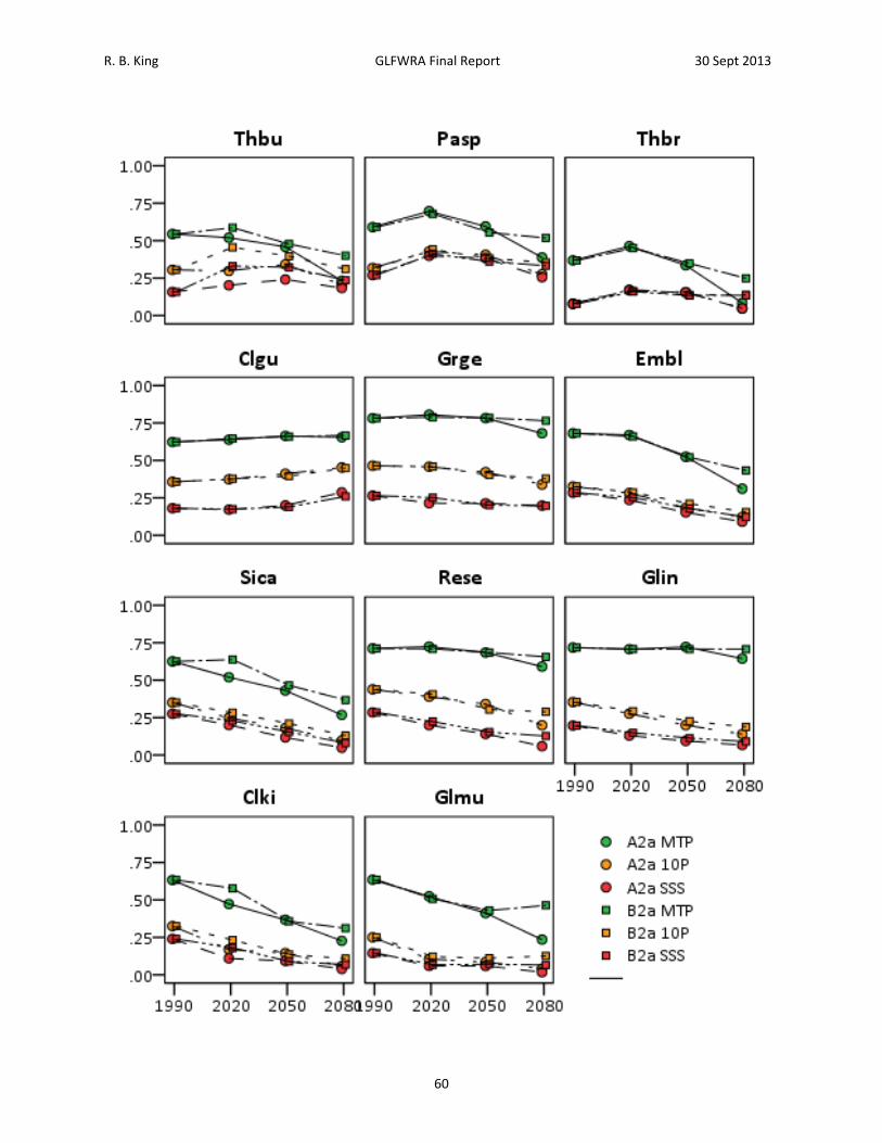
R. B. King GLFWRA Final Report 30 Sept 2013
60
R. B. King GLFWRA Final Report 30 Sept 2013
61
Discussion Predicting species’ responses to climate change is challenging and consequently, appropriate management strategies are uncertain (Rodŕiguez‐Castañeda et al. 2012). Here, this uncertainty was minimized by considering climate change impacts on multiple co‐distributed species simultaneously, making it possible to distinguish among species that may be affected by climate change to a lesser or greater degree even if the magnitude of those effects is uncertain. Furthermore, by restricting the geographic scope of analyses, overfitting of environmental niche models was reduces, resulting in more accurate projections of climate change impacts within currently occupied and adjacent locations. Association between climatic variables and current distributions. – Current distributions of reptiles of conservation concern in the Great Lakes region were well predicted by ecological niche models that incorporated four to seven Bioclim variables (Table 5, Fig. 4‐14). For all species, mean annual temperature (Bio1) consistently ranked high among variables included in the models (Table 5). With the exception of Thamnophis brachystoma, response curves for this variable were unimodal convex in shape (Table 6, Fig. 15), suggesting that both low and high mean temperatures may limit species distributions. Mean diurnal temperature range (Bio2) and annual precipitation (Bio12) were also included in models for all species but response curves for these variable were inconsistent in shape (Table 5, 6). Temperature isothermality (Bio 3) and several variables relating to precipitation (Bio13 – precipitation in the wettest month, Bio14 – precipitation in the driest month, Bio 15 – precipitation sesonality) contributed to models for some species, but again, the shape of response curves varied among species (Table 5, 6). Modelers frequently use different sets of candidate climatic variables and this makes it difficult to directly compare results obtained here with environmental niche models for other reptile species. However, variables related to temperature and precipitation are frequent contributors (e.g., red‐eared slider, Kikillus et al. 2010; boid snakes, DiCola et al. 2008; smooth snake, Santos et al. 2009; brown tree snake, Rödder and Lotter 2010; Plain‐bellied Watersnake, Makowsky et al. 2010; African viperids, Brito et al. 2011; turtles world‐wide, Ihlow et al. 2012; a Mediterranean viper, Brito et al. 2011; Burmese pythons, Rodda et al. 2011). Annual degree days, a correlate of mean annual temperature, is an important contributor to an ecological niche model of Orsini’s Viper and exhibits a unimodal convex response curve much like seen in this study for mean annual temperature (Lyet et al. 2013). One species included in the present analysis, the Eastern Massasauga Sistrurus catenatus catenatus, was the focus of a previous ecological niche model aimed at understanding niche divergence among Sistrurus species and subspecies (Wooten and Gibbs 2011). Four other species were the focus of an analysis of climate change impacts on turtle species world‐wide (Ihlow et al. 2012). The percent contribution of Bioclim variables differs somewhat between models for these species (Table 9). However, for the Eastern Massasauga, areas of high climatic suitability correspond closely (compare ther Fig. 2b in Wooten and Gibbs 2011 with Fig. 10A in this report); comparable maps are not available from Ihlow et al. (2012).
R. B. King GLFWRA Final Report 30 Sept 2013
62
Projected future location of areas of high climatic suitability. – Reptiles of conservation concern in the Great Lakes regions consistently show projected reductions in climatic suitability at locations currently occupied (Fig. 16) and most show reductions in climatic suitability within the region more generally (Fig. 17). In general, reductions in climatic suitability first become evident in the southern and western portions of species’ ranges (Fig. 4‐14). Species differ in the time‐frame over which climate change impacts are projected to occur with some species not showing marked declines in climatic suitability until 2080 (Thamnophis butleri, Pantherophis sp., Thamnophis brachystoma; Fig. 16). Other species show linear declines in climatic suitability from the present through 2080 (Clemmys guttata, Graptemys geographica, Emydoidea blandingii, Sistrurus catenatus catenatus, Regina septemvitta; Fig. 16). Still other species show immediate rapid declines in climatic suitability (e.g., from the present through 2020 or 2050) with a decreasing rate of decline thereafter (Glyptemys insculpta, Clonophis kirtlandii, Glyptemys muhlenbergii; Fig. 16). The degree to which new areas of high climatic suitability arise also varies among species. Areas currently occupied by Thamnophis butleri, Pantherophis sp., Thamnophis brachystoma, and Clemmys guttata show decreases vs. constancy or increases in climatic suitability in roughly equal numbers of states and provinces (Table 10). These species are also projected to experience increased climatic suitability outside of their current distribution in a notable number of states and provinces (Table 10). In some cases, these new areas of high climatic suitability appear in states and provinces not currently occupied (Pantherophis sp., Thamnophis brachystoma, Clemmys guttata; Table 10). Most other species show decreases in climatic suitability in most states and provinces in which they currently occur and relatively few or no unoccupied states or provinces where new areas of high climatic suitability arise (e.g., Emydoidea blandingii in parts of Ontario only, Sistrurus catenatus in parts of Ontario and Quebec only, Glyptemys insculpta not at all; Table 10). Ecological niche models have been used to predict responses of reptiles to climate change only infrequently. However, declines in climatic suitability similar to that reported here is predicted in the endangered Australian snake, Hoplocephalus bungaroids (Penman et al. 2010) in which just 14% of current sites are remain climatically suitable in 2070 under a high warming scenario. Similarly, the Mediterranean viper, Vipera latasei, is projected to experience declines in climatic suitability over 57% of its core habitat (Brito et al. 2011). In an analysis of 199 turtle species world‐wide, Ihlow et al. (2012) project that 86% of species may experience climate‐change induced range contraction by 2080. Similarly, climate change is projected to induce displacement of 11 North American rattlesnake species by 430‐2,420 m/yr (Lawing and Polly 2011). Prioritization of species and associated management, research, and policy actions. – Based on projections presented here, reptiles of conservation concern in the Great Lakes region differ in their susceptibility to climate change. Based on projections of the proportion of known localities falling above the SSS threshold under the A2a scenario in 2050, Thamnophis butleri,
R. B. King GLFWRA Final Report 30 Sept 2013
63
Pantherophis species, and Thamnophis brachystoma are least sensitive to climate change; greater than 75% of their known localities are projected to remain climatically suitable (Table 6, Fig. 16). Furthermore, these species may benefit from the appearance of new areas of high climatic suitability that are not currently occupied, at least in the near term (Table 7, Fig. 17). Clemmys guttata and Graptemys geographica are somewhat more sensitive; 50‐75% of known localities are projected to remain climatically suitable and the area of high climatic suitability remains relatively constant (Table 7, Fig. 17). The remaining species appear to be highly sensitive to climate change. Emydoidea blandingii, Sistrurus catenatus catenatus, and Regina septemvittata are projected to have 25‐50% of known localities remain climatically suitable and Clonophis kirtlandii, Glyptemys insculpta, and Glyptemys muhlenbergii are projected to have less than 25% of known localities remain climatically suitable (Table 6, Fig. 16). These species also show steadily declining areas of high climatic suitability, whether those areas are occupied or not (Table 7, Fig. 17). Among the species included in this analysis, projected effects of climate change do not appear to be greater for species with more restricted distributions (e.g., compare Thamnophis brachystoma, a species with an extremely limited geographic distribution for which climatic suitability is projected to remain high, and Regina septemvittata a species with a broad geographic distribution for which climatic suitability is projected to decrease over much of its range). In addition to these species‐specific projections, it is useful to summarize these trends by state or province because management, research and policy are often set at the state and provincial level (Table 11). One pattern that emerges from such a summary is that most states and provinces listed are home to one or more unprotected species for which climatic suitability is projected to decrease (exceptions include MI, NH, NJ, ON, QU, RI, VT). Another pattern that is evident is that there a number of states and provinces not currently occupied by given species where new areas of high climatic suitability are projected to arise (i. e. KY, MD, NJ, NY, ON, PA, QU, VA, WI, WV). Species‐specific (Table 10) and state/province‐specific (Table 11) trends in climatic suitability have immediate implications for management, research, and policy actions identified previously (Fig. 18). High priority species (those projected to be most sensitive to climate change) include Emydoidea blandingii, Sistrurus catenatus catenatus, Regina septemvittata, Clonophis kirtlandii, Glyptemys insculpta, and Glyptemys muhlenbergii. Because these species are projected to experience decreased climatic suitability in some occupied locations, constant or increased climatic suitability in other occupied locations (except Sistrurus catenatus catenatus), and increases climatic suitability in some unoccupied locations (except Glyptemys insculpta), a wide range of management, research, and policy actions are warranted across multiple states and provinces (Fig. 18). Importantly, many of these actions (e.g., population monitoring and habitat management) serve ‘double duty’ in that they represent appropriate responses to threats arising from habitat loss, overexploitation, and invasive species as well as the added threat posed by climate change.
R. B. King GLFWRA Final Report 30 Sept 2013
64
Population monitoring efforts focused on areas where climatic suitability is projected to decline most rapidly would aid in the early detection and timely response to climate change impacts (e.g., Emydoidea blandingii in IA, IN, OH,, MN, and NE; Sistrurus catenatus catenatus in IL, IN and WI; RESE in AL, GA, KY, IL, IN, and OH; Clonophis kirtlandii in IL and IN; Glyptemys muhlenbergii in NC, PA, and VA). Recent research provides an incomplete understanding of the degree and mechanisms of climate change induced effects on reptiles but does point to anticipated changes in behavior (Refsnider and Janzen 2012; Refsnider et al. 2013; Weatherhead et al. 2012), offspring sex ratios ( Mitchell and Janzen 2010; Refsnider and Janzen 2012; Refsnider et al. 2013), reproductive physiology and phenology (Lourdais et al 2004; Moasterio et al. 2013; Telemeco et al. 2013), and life history (Ujvari et al. 2011). Thus, it would be beneficial to combine monitoring efforts with research on individual‐ and population‐level phenomena (e.g., age‐ and size‐specific growth, reproduction and mortality; realized population growth rates) to aid in refining management strategies. Synergistic effects of climate change and other stressors also warrant consideration (Rohr and Palmer 2013). Other actions are more specific to the threat of climate change alone. For example, of the high priority species listed above, formal recognition as endangered, threatened, or of special concern is sometimes lacking in some states projected to decrease in climatic suitability (e.g., Regina septemvittata in AL, DE, FL, GA, IL, IN, KY, MD, NC, SC, TN, VA, and WV; Clonophis kirtlandii in KY; Glyptemys insculpta in DE, MD, and ME). For other species, recognition exists but may be insufficient. An interesting example is the Blanding’s Turtle, Emydoidea blandingii. This species is recognized as threatened or endangered throughout much of its range but only as a species of special concern in Nebraska, where large populations persist in several areas (Congdon et al. 2008). However, this analysis suggests that Nebraska populations are especially vulnerable to climate change (Fig. 9). Blanding’s Turtles also appear vulnerable to climate change in Wisconsin (Fig. 9) where an administrative rule process to delist this species is underway (http://dnr.wi.gov/topic/endangeredresources/etlist.html). Even if additional protection were not deemed necessary, including these species in Natural Heritage database compilations of element occurrence records would provide valuable baseline data from which climate change impacts could be inferred. Identifying new areas of high climatic suitability is a strength of environmental niche modeling and has particular utility for informing conservation management decisions (Schwartz 2012). Here, the projection that new areas of climatic suitability will arise means that a number of states and provinces face the possibility of natural or facilitated colonization of currently unoccupied areas (e.g., Emydoidea blandingii in currently unoccupied parts of ON; Sistrurus catenatus catenatus in ON and QU; Regina septemvittata in NY, ON, and WI; Clonophis kirtlandii in NY, ON, and PA; Glyptemys muhlenbergii in ON and QU). Policy decisions regarding the desirability of range expansion, together with research on habitat suitability and dispersal mechanisms may be necessary steps in these cases. The extension of existing habitat utilization and suitability models (Emydoidea blandingii – Millar and Blouin‐Demers 2011, Paterson et al. 2012; Sistrurus catenatus catenatus – Bailey et al. 2012; DeGregorio et al. 2011; Glyptemys insculpta – Paterson et al. 2012; Glyptemys muhlenbergii – Feaga et al. 2012) to new areas of climatic suitability would aid in evaluating the likely success of natural or assisted colonization.
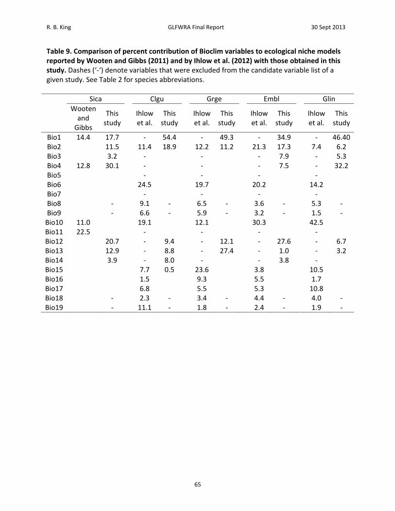
R. B. King GLFWRA Final Report 30 Sept 2013
65
Table 9. Comparison of percent contribution of Bioclim variables to ecological niche models reported by Wooten and Gibbs (2011) and by Ihlow et al. (2012) with those obtained in this study. Dashes (‘‐‘) denote variables that were excluded from the candidate variable list of a given study. See Table 2 for species abbreviations.
Sica Clgu Grge Embl Glin
Wooten and Gibbs
This study
Ihlow et al.
This study
Ihlow et al.
This study
Ihlow et al.
This study
Ihlow et al.
This study
Bio1 14.4 17.7 ‐ 54.4 ‐ 49.3 ‐ 34.9 ‐ 46.40Bio2 11.5 11.4 18.9 12.2 11.2 21.3 17.3 7.4 6.2 Bio3 3.2 ‐ ‐ ‐ 7.9 ‐ 5.3 Bio4 12.8 30.1 ‐ ‐ ‐ 7.5 ‐ 32.2 Bio5 ‐ ‐ ‐ ‐ Bio6 24.5 19.7 20.2 14.2 Bio7 ‐ ‐ ‐ ‐ Bio8 ‐ 9.1 ‐ 6.5 ‐ 3.6 ‐ 5.3 ‐ Bio9 ‐ 6.6 ‐ 5.9 ‐ 3.2 ‐ 1.5 ‐ Bio10 11.0 19.1 12.1 30.3 42.5 Bio11 22.5 ‐ ‐ ‐ ‐ Bio12 20.7 ‐ 9.4 ‐ 12.1 ‐ 27.6 ‐ 6.7 Bio13 12.9 ‐ 8.8 ‐ 27.4 ‐ 1.0 ‐ 3.2 Bio14 3.9 ‐ 8.0 ‐ ‐ 3.8 ‐ Bio15 7.7 0.5 23.6 3.8 10.5 Bio16 1.5 9.3 5.5 1.7 Bio17 6.8 5.5 5.3 10.8 Bio18 ‐ 2.3 ‐ 3.4 ‐ 4.4 ‐ 4.0 ‐ Bio19 ‐ 11.1 ‐ 1.8 ‐ 2.4 ‐ 1.9 ‐
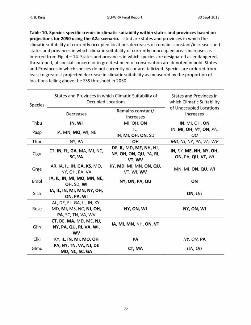
R. B. King GLFWRA Final Report 30 Sept 2013
66
Table 10. Species‐specific trends in climatic suitability within states and provinces based on projections for 2050 using the A2a scenario. Listed are states and provinces in which the climatic suitability of currently occupied locations decreases or remains constant/increases and states and provinces in which climatic suitability of currently unoccupied areas increases as inferred from Fig. 4 – 14. States and provinces in which species are designated as endangered, threatened, of special concern or in greatest need of conservation are denoted in bold. States and Provinces in which species do not currently occur are italicized. Species are ordered from least to greatest projected decrease in climatic suitability as measured by the proportion of locations falling above the SSS threshold in 2050.
Species
States and Provinces in which Climatic Suitability of Occupied Locations
States and Provinces in which Climatic Suitability of Unoccupied Locations
Increases Decreases Remains constant/
Increases
Thbu IN, WI MI, OH, ON IN, MI, OH, ON
Pasp IA, MN, MO, WI, NE IL,
IN, MI, OH, ON, SD IN, MI, OH, NY, ON, PA,
QU
Thbr NY, PA OH MD, NJ, NY, PA, VA, WV
Clgu CT, IN, FL, GA, MA, MI, NC,
SC, VA
DE, IL, MD, ME, NH, NJ, NY, OH, ON, QU, PA, RI,
VT, WV
IN, KY, ME, NH, NY, OH, ON, PA, QU, VT, WI
Grge AR, IA, IL, IN, GA, KS, MO,
NY, OH, PA, VA KY, MD, MI, MN, ON, QU,
VT, WI, WV MN, MI, ON, QU, WI
Embl IA, IL, IN, MI, MO, MN, NE,
OH, SD, WI NY, ON, PA, QU ON
Sica IA, IL, IN, MI, MN, NY, OH,
ON, PA, WI ON, QU
Rese AL, DE, FL, GA, IL, IN, KY, MD, MI, MS, NC, NJ, OH,
PA, SC, TN, VA, WV NY, ON, WI NY, ON, WI
Glin CT, DE, MA, MD, ME, NJ, NY, PA, QU, RI, VA, WI,
WV
IA, MI, MN, NH, ON, VT
Clki KY, IL, IN, MI, MO, OH PA NY, ON, PA
Glmu PA, NY, TN, VA, NJ, DE
MD, NC, SC, GA CT, MA ON, QU
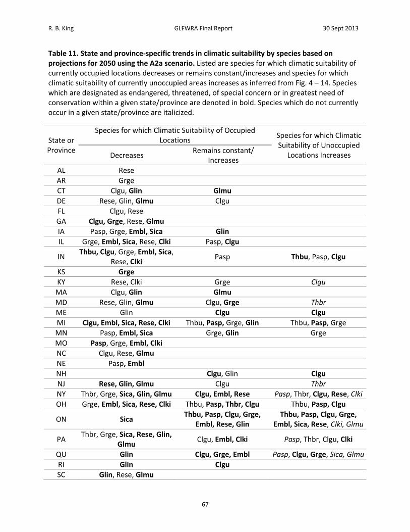
R. B. King GLFWRA Final Report 30 Sept 2013
67
Table 11. State and province‐specific trends in climatic suitability by species based on projections for 2050 using the A2a scenario. Listed are species for which climatic suitability of currently occupied locations decreases or remains constant/increases and species for which climatic suitability of currently unoccupied areas increases as inferred from Fig. 4 – 14. Species which are designated as endangered, threatened, of special concern or in greatest need of conservation within a given state/province are denoted in bold. Species which do not currently occur in a given state/province are italicized.
State or Province
Species for which Climatic Suitability of Occupied Locations
Species for which Climatic Suitability of Unoccupied
Locations Increases Decreases Remains constant/
Increases
AL Rese
AR Grge
CT Clgu, Glin Glmu
DE Rese, Glin, Glmu Clgu
FL Clgu, Rese
GA Clgu, Grge, Rese, Glmu
IA Pasp, Grge, Embl, Sica Glin
IL Grge, Embl, Sica, Rese, Clki Pasp, Clgu
IN Thbu, Clgu, Grge, Embl, Sica,
Rese, Clki Pasp Thbu, Pasp, Clgu
KS Grge
KY Rese, Clki Grge Clgu
MA Clgu, Glin Glmu
MD Rese, Glin, Glmu Clgu, Grge Thbr
ME Glin Clgu Clgu
MI Clgu, Embl, Sica, Rese, Clki Thbu, Pasp, Grge, Glin Thbu, Pasp, Grge
MN Pasp, Embl, Sica Grge, Glin Grge
MO Pasp, Grge, Embl, Clki
NC Clgu, Rese, Glmu
NE Pasp, Embl
NH Clgu, Glin Clgu
NJ Rese, Glin, Glmu Clgu Thbr
NY Thbr, Grge, Sica, Glin, Glmu Clgu, Embl, Rese Pasp, Thbr, Clgu, Rese, Clki
OH Grge, Embl, Sica, Rese, Clki Thbu, Pasp, Thbr, Clgu Thbu, Pasp, Clgu
ON Sica Thbu, Pasp, Clgu, Grge,
Embl, Rese, Glin Thbu, Pasp, Clgu, Grge,
Embl, Sica, Rese, Clki, Glmu
PA Thbr, Grge, Sica, Rese, Glin,
Glmu Clgu, Embl, Clki Pasp, Thbr, Clgu, Clki
QU Glin Clgu, Grge, Embl Pasp, Clgu, Grge, Sica, Glmu
RI Glin Clgu
SC Glin, Rese, Glmu
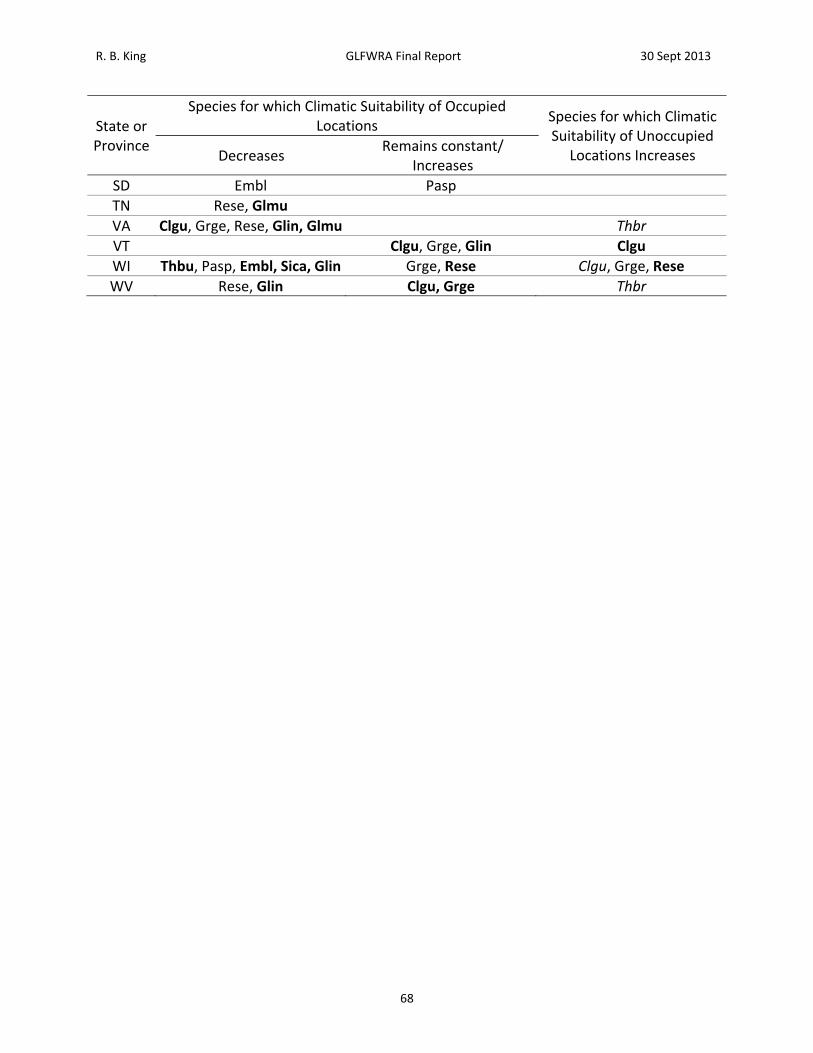
R. B. King GLFWRA Final Report 30 Sept 2013
68
State or Province
Species for which Climatic Suitability of Occupied Locations
Species for which Climatic Suitability of Unoccupied
Locations Increases Decreases Remains constant/
Increases
SD Embl Pasp
TN Rese, Glmu
VA Clgu, Grge, Rese, Glin, Glmu Thbr
VT Clgu, Grge, Glin Clgu
WI Thbu, Pasp, Embl, Sica, Glin Grge, Rese Clgu, Grge, Rese
WV Rese, Glin Clgu, Grge Thbr
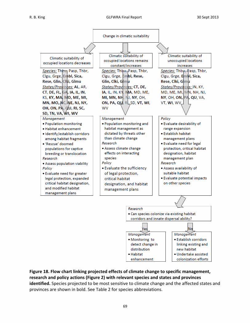
R. B. King GLFWRA Final Report 30 Sept 2013
69
Figure 18. Flow chart linking projected effects of climate change to specific management, research and policy actions (Figure 2) with relevant species and states and provinces identified. Species projected to be most sensitive to climate change and the affected states and provinces are shown in bold. See Table 2 for species abbreviations.
R. B. King GLFWRA Final Report 30 Sept 2013
70
Acknowledgements A project of this nature is only possible through the cooperation of curators and collections managers of specimen and data repositories and the institutions they represent. Tthe significant contributions of institutions, agencies and personnel listed in Table 1, including N. Baker, M. Barbour, D. Becker, N. Bradley, S. Bump, D. Butler, S. Cairns, J. Campbell, D. Cannatella, R. Craig, J. Davis, J. Delisle, D. Dickey, T. Erdman, G. Fowles, C. Franklin, D. Frost, S. H. Gerriets, J. Giermakowski, N. Gilmore, D. Gregg, B. Gray, R. Hellmich, S. Hines, J. Holling, D. Howell, J. Jacobs, R. Jones, T. Kieninger, D. Kizirian, K. Kozak, K. Krysko, T. Labedz, T. LaDuc, Y. Lee, A. Luxbacher, M. Mahoney, C. Mayer, G. Mayer, H. Mays, N. McCartney, W. Meshaka, S. Miller, S. Moody, R. Muehlheim, A. Nelson, R. Nussbaum, M. O'Brien, C. Osborne, A. Paquet, C. Phillips, A. Resetar, L. Rissler, D. Roberts, R. Rogers, B. Sargent, C. Schmidt, G. Schneider, R. Schneider, G. Schneider, A. Scott, R. Simpson, J. Sites, W. Skidmore, H. Snell, E. Stetzar, S. Sullivan, M. Suter, K. Tighe, T. Warf, E. Wild, K. Zyko are gratefully acknowledged. E. Hileman, C. Jaeger, and G. Rodda provided helpful discussions during the development and completion of this project. Northern Illinois University and the NIU Department of Biological Sciences provided financial and logistic support. Partial funding for this program came from a Grant Agreement from the U.S. Department of the Interior, Fish and Wildlife Service. Mention of trade names or commercial products does not constitute their endorsement by the U.S. Government. Literature Cited Acevedo, P., A. Jiménez‐Valverde, J. M. Lobo, and R. Real. 2012. Delimiting the geographical
background in species distribution modelling. Journal of Biogeography 39: 1383–1390. Ackerly, D.D., S.R. Loarie, W.K. Cornwell., S.B. Weiss, H. Hamilton, R. Branciforte, and J.J.B.
Kraft. 2010. The geography of climate change: implications for conservation biogeography. Diversity and Distributions 16:476‐487.
Araújo, M.B., and R.G. Pearson. 2005. Equilibrium of species’ distributions with climate. Ecography 28:693‐695.
Bailey, R. L., H. Campa, K. M. Bissell, and T. M. Harrison. 2012. Resource selection by the eastern massasauga rattlesnake on managed land in southwestern Michigan. Journal of Wildlife Management 76:414‐421.
Bennett, A. M., M. Keevil, and J. D. Litzgus. 2010. Spatial ecology and population genetics of Northern Map Turtles (Grapytemys geographica) in fragmented and continuous habitats in Canada. Chelonian Conservation and Biology 9:185‐195.
Bennie, J., J. A. Hodgson, C. R. Lawson, C. T. R. Holloway, D. B. Roy, T. Brereton, C. D. Thomas, and R. J. Wilson. 2013. Range expansion through fragmented landscapes under a variable climate. Ecology Letters 16:921‐929.
Brodman, R. 2009. A 14‐year study of amphibian popualtions and metacommunities. Herpetological Conservation and Biology 4:106‐119.
Brito, J. C., S. Fahd, P. Geniez, F. Martínez‐Freiría, J. M. Pleguezuelos, and J. –F. Trape. 2011. Biogeography and conservation of viperids from North‐West Africa: an application of ecological niche‐based models and GIS. Journal of Arid Environments 75:1029‐1037.
R. B. King GLFWRA Final Report 30 Sept 2013
71
Brito, J. C., S. Fahd, P. Geniez, F. Martínez‐Freiría, P. tarroso, S. Larbes, J. M. Pleguezuelos, and X. Santos. 2011. Climate change and peripheral populations: predictions for a relicth Mediterranean viper. Acta Herpetologica 6:105‐118.
Cao, Y., R. E. DeWalt, J. L. Robinson, T. Tweddale, L. Hinz, and M. Pessino. 2013. Using Maxent to model the historic distributions of stonefly species in Illinois streams: the effects of regularization and threshold selections. Ecological Modelling 259:30–39.
Chauvenet, A. L. M., J. G. Ewen, D. P. Armstrong, T. M. Blackburn, and N. Pettorelli. 2012. Maximizing the success of assisted colonizations. Animal Conservation 16:161‐169.
Collins, J. T. 1991. Viewpoint: a new taxonomic arrangement for some North American amphibians and reptiles. Herpetolgical Review 22:42–43.
Conant, R. and Collins, J. T. 1991. A Field Guide to Reptiles and Amphibians: Eastern and Central North America (Peterson Field Guides). Houghton Mifflin Company.
Congdon, J. D., T. E. Graham, T. B. Herman, J. W. Lang, M. J. Pappas, and B. J. Brecke. 2008. Emydoidea blandingii (Holbrook 1838) ‐ Blading's turtle. In A. G. J. Rhodin, P. C. H. Pritchard, P. P. van Dijk, R. A. Saumure, K. A. Buhlmann, and J. B. Iverson, editors. Conservation biology of freshwater turtles and tortoises: a compilation project of the IUCN/SSC tortoise and freshwater turtle specialist group. Chelonian Research Monographs No. 5, pp 05.1‐015.12. Chelonian Research Foundation.
Crother, B. I. (ed.). 2008. Scientific and Standard English Names of Amphibians and Reptiels of North America North of Mexico. Pp 1‐84. SSAR Herpetological Circular 37.
Crother, B.I., M.E. White, J.M. Savage, M.E. Eckstut, M.R.Graham, and D.W. Gardner. 2011. A reevaluation of the status of the fox snakes Pantherophis gloydi Conant and P. vulpinus Baird and Girard (Lepidosauria). ISRN Zoology, Article ID 436049, 15 pages. doi:10.5402/2011/436049.
DeGregorio, B. A., B. J. Putman, and B. A. Kingsbury. 2011. Which habitat selection method is most applicable to snakes? Case studies of the Eastern Massasuaga (Sistururus catenatus) and Eastern Fox Snake (Pantherophis gloydi). Herpetological Conservation and Biology 6:372‐382.
Di Cola, V., G. Cardozo, M. Lanfri, C. M. Scavuzzo, and M. Chiaraviglio. 2008. Modelling the distribution of the Boid snakes, Epicrates cenchria alvarezi and Boa constrictor occidentalis in the Gran Chaco (South America). Amphibia‐Reptilia 29:299‐310.
DiLeo, M. F., J. R. Row, and S. C. Lougheed. 2010. Discordant patterns of population structure for two co‐distributed snake species across a fragmented Ontario landscape. Diversity and Distributions 16:571‐591.
Deutsch, C.A., J.J. Tewksbury, R.B. Huey, K.S. Sheldon, C.K. Ghalambor, D.C. Haak, P.R. Martin. 2008. Impacts of climate warming on terrestrial ectotherms across latitude. PNAS 105: 6668‐6672.
Doody, J. S., and J. A. Moore. 2010. Conceptual model for thermal limits on the distribution of reptiles. Herpetological Conservation and Biology 5:283‐289.
Elith, J., C. H. Graham, R. P. Anderson, M. Dudík, S. Ferrier, A. Guisan, R. J. Hijmans, F. Huettmann, J. R. Leathwick, A. Lehmann, J. Li, L. G. Lohmann, B. A. Loiselle, G. Manion, C. Moritz, M. Nakamura, Y. Nakazawa, J. McC. Overton, A. T. Peterson, S. J. Phillips, K. Richardson, R. Scachetti‐Pereira, R. E. Schapire, J. Soberón, S. Williams, M. S. Wisz, and N.
R. B. King GLFWRA Final Report 30 Sept 2013
72
E. Zimmerman. 2006. Novel methods improve predictions of species’ distributions from occurrence data. Ecography 29:129‐151, 2006.
Enneson, J.J., and J.D. Litzgus. 2009. Stochastic and spatially explicit population viability analysis for an endangered freshwater turtle, Clemmys guttata. Canadian Journal of Zoology 87:1241‐1254.
Ewert, M. A., and Nelson, C. E. 1991. Sex determination in turtles: diverse patterns and some possible adaptive values. Copea 1991:50‐69.
Fang, F. , H. Sun, Q. Zhao, C. Lin, Y. Sun, W. Gao, J. Xu, J. Zou, F. Ge, and N. Lu. 2013. Patterns of diversity, areas of endemism, and multiple glacial refuges for freshwater crabs of the genus Sinopotamon in China (Decapoda: Brachyura: Potamidae). PLoS ONE 8: e53143.
Feaga, J. B., C. A. Haas, and J. A. Burger. Water table depth, surface saturation, and drought response in bog turtle (Glyptemys muhlenbergii) wetlands. Wetlands 32:1011‐1021.
Francl, K. E., K. Hayhoe, M. Saunders, and M. P. Maurer. 2009. Ecosystem adaptation to climate change: small mammal migration pathways in the Great Lakes states. Journal of Great Lakes Research 36:86‐93.
Franklin, J. 2010. Moving beyond static species distribution models in support of conservation biogeography. Diversity and Distributions 16:321‐330.
Galatowitsch, S., L. Frelich, and L. Phillips‐Mao. 2009. Regional climate change adaptation strategies for biodiversity conservation in a midcontinental region of North America. Biological Conservation 142:2012‐2022.
Gibbs HL, Murphy M, Chiucchi JE. 2010. Genetic identity of endangered massasauga rattlesnakes (Sistrurus sp.) in Missouri. Conservation Genetics 12:433–439.
Harding, J. H. 1997. Amphibians and Reptiles of the Great Lakes Region. The University of Michigan Press. Ann Arbor, MI.
Hedrick, P.W. 2005. "Genetic restoration": a more comprehensive perspective than "genetic rescue." Trends in Ecology and Evolution 20:109.
Hickling, R., D.B. Roy, J.K. Hill, R. Fox, and C.D. Thomas. 2006. The distributions of a wide range of taxonomic groups are expanding polewards. Global Change Biology 12:450‐455.
Hijmans, R.J., S.E. Cameron, J.L. Parra, P.G. Jones and A. Jarvis, 2005. Very high resolution interpolated climate surfaces for global land areas. International Journal of Climatology 25:1965‐1978.
Hijmans, R.J. and Graham, C.H. 2006. The ability of climate envelope models to predict the effect of climate change on species distributions. Global Change Biology 12:1‐10.
Huey, R. B. 1982. Temperature, phsiolology and the ecology of reptiles. In C. Gans and F. H. Pough (eds.), Biology of the Reptila, Volume 12: Physiology C‐Physiological Ecology. Academic Press, London.
Ihlow, F. ,J. Damback, J. O. Engler, M. Flecks, T. Harmann, S. Nekum, H. Rajaei, and D. Rödder. 2012. On the brink of extinction? How climate change may affect global chelonian species richness and distribution. Global Change Biology 18:1520–1530.
Intergovernmental Panel on Climate Change (IPCC) 2007. IPCC Special Report on Emissions Scenarios (SRES) Emissions Scenarios Dataset Version 1.1 New York, NY: Cambridge University Press.
R. B. King GLFWRA Final Report 30 Sept 2013
73
Kikillus, K. H., K. M. Hare, and S. Hartley. 2010. Minimizing false‐negatives when predictiong the potential distribution of an invasive species: a bioclimatic envelope for the red‐eared slider at global and regional scales. Animal Conservation 13 (Suppl. 1):5‐15.
Klaus, S. P., and S. C. Lougheed. 2013. Changes in breeding phenology of eastern Ontario frogs over four decades. Ecology and Evolution 3:835‐845.
Kramer‐Schadt, S., J. Niedballa, J. D. Pilgrim, B. Schröder, J. Lindeborn, V. Reinfelder, M. Stillfried, I. Heckmann, A. K. Scharf, D. M. Augeri, S. M. Cheyne, A. J. Hearn, J. Ross, D. W. Macdonald, J. Mathai, J. Eaton, A. J. Marshall, G. Semiadi, R. Rustam, H. Bernard, R. Alfred, H. Samejima, J. W. Duckworth, C. Breitenmoser_Wuersten, J. L. Belant, H. Hofer, and A. Wilting. 2013. The importance of correcting for sampling bias in MaxEnt species distribution models. Diversity and Distributions. Doi:10.1111/ddi.12096.
Kubatko LS, Gibbs HL, Bloomquist EW. 2011. Inferring species–level phylogenies and taxonomic distinctiveness using multilocus data in Sistrurus rattlesnakes. Systematic Biology 60:393–409.
Kumar, S. and Stohlgren, T. J. 2009. Maxent modeling for predicting suitable habitat for threatened and endangered tree Canacomyrica monticola in New Caledonia. Journal of Ecology and Natural Environment 1:94–98.
Lawing, A. M., and P. D. Polly. 2011. Pleistocene climate, phylogeny, and climate envelope models: an integrative approach to better understand species’ response to climate change. PLoS ONE 6: e28554. doi:10.1371/journal.pone.0028554.
Lourdais, O., R. Shine, X. Bonnet, M. Guillon, and G. Naulleau. 2004. Climate affects embryonic development in a viviparous snake, Vipera aspis. Oikos 104:551‐560.
Lyet, A., W. Thuiller, M. Cheylan, and A. Besnard. 2013. Fine‐scale regional distribution modeling of rare and threatened species: bridging GIS tools and conservation in practice. Diversity and Distributions 19:651‐663.
Makowsky, R., J. C. Marshall Jr., J. McVay, P. T. Chippendale, and L. J. Rissler. 2010. Phylogenetic analysis and environmental modeling of the plain‐bellied watersnake (Nerodia erythrogaster) reveals low levels of genetic and ecological differentiation. Molecular Phylogentics and Evolution 55:985‐995.
Millar, C. S., and G. Blouin‐Demers. 2012. Habitat suitability modeling for species at risk is sensitive to algorithm and scale: a case study of Blanding’s turtle, Emydoidea blandingii, in Ontario, Canada. Journal for Nature Conservation 20:18‐29.
Mitchell, N. J., and F. J. Janzen. 2010. Temperature‐dependent sex determination and contemporary climate change. Sexual Development 4:129‐140.
Mockford, S. W., T. B. Herman, M. Snyder, and J. M. Wright. 2007. Conservation genetics of Blanding’s turtle and its application to the identification of evolutionary significant units. Conservation Genetics 8:209‐219.
Monasterio, C., L. P. Shoo, a. Salvador, P. Iraeta, and J. A. Díaz. 2013. High temperature constrains reproductive success in a temperate lizard: implications for distributions range limits and the impacts of climate change. Journal of Zoology 291:136‐145.
Moreno‐Rueda, G., J. M. Pleguezuelos, M. Pizarro, and A. Montori. 2011. Northward shifts of the distributions of Spanish reptiles in association with climate change. Conservation Biology 26:278‐283.
R. B. King GLFWRA Final Report 30 Sept 2013
74
Myers, P., B. L. Lundrigan, S. M. G. Hoffman, A. P. Haraminac, and S. H. Seto. 2009. Climate‐induced changes in small mammal communities of the Northern Great Lakes Region. Global Change Biology 15:1434‐1454.
Owens, H. L., L. P. Campbell, L. L. Dornack, E. E. Saupe, N. Barve, J. Soberón, K. Ingeloff, a. Lira‐Noriega, C. M. Hensz, C. E. Myers, and A. T. Peterson. 2013. Ecological Modelling 263:10‐18.
Panella, M. J. 2012. Blanding’s Turtle (Emydoidea blandingii); a species conservation assessment for the Nebraska Natural Legacy Project. Nebraska Game and Parks Commission, Wildlife Division. 13 pp.
Paterson, J. E., B. D. Steinberg, and J. d. Litzgus. 2012. Revealing a cryptic life‐history stage: differences in habitat selection and survivorship between hatchlings of two turtle speces at risk (Glyptemys insulpta and Emydoidea blandingii). Wildlife Research 39:408‐418.
Pearson, R.G., Raxworthy, C.J., Nakamura, M., and Peterson, A.T. 2007. Predicting species distributions from small numbers of occurrence records: a test case using cryptic geckos in Madagascar. Journal of Biogeography 34:102‐117.
Penman, T.D., D.A. Pike, J.K. Webb, and R. Shine. 2010. Predicting the impact of climate change on Australia’s most endangered snake, Hoplocephalus bungaroides. Diversity and Distributions 16:109‐118.
Phillips, S. J. and Dudík, M. 2008. Modeling of species distributions with Maxent: new extensions and a comprehensive evaluation. Ecography 31:161–175.
Phillips, S.J., R.P. Anderson, and R.E. Schapire. 2006. Maximum entropy modeling of species geographic distributions. Ecological Modeling 190:213‐259.
Povilitis, A., and K. Suckling. 2010. Addressing climate change threats to endangered species in U.S. recovery plans. Conservation Biology 24:372‐376.
Ramirez, J. and Jarvis, A. 2008. High Resolution Statistically Downscaled Future Climate Surfaces. International Center for Tropical Agriculture (CIAT); CGIAR Research Program on Climate Change, Agriculture and Food Security (CCAFS). Cali, Colombia.
Ray, J.W., R.B. King, M.R. Duvall., J.W. Robinson, M.J. Dreslik, B.J. Swanson, and D. Mulkerin. 2012. Genetic analysis and captive breeding program design for the Eastern Massasauga Sistrurus catenatus catenatus. Journal of Fish and Wildlife Management 4:104‐113. Available at http://www.fwspubs.org/toc/fwma/0/0.
Refsnider, J. M., and F. J. Janzen. 2012. Behavioural plasticity may compensate for climate change in a long‐lived reptile with temperature‐dependent sex determination. Biological Conservation 152:90‐95.
Refsnider, J. M., B. L. Bodensteiner, J. L. Reneker, and F. J. Janzen. 2013. Nest depth may not compensate for sex ratio skews caused by climate change in turtles. Animal Conservation 16: DOI: 10.1111/acv.12034.
Rodda, G.H., C.S. Jarnevich, and R.N. Reed. 2011. Challenges in identifying sites climatically matched to the native ranges of animal invaders. PloS One 6(2):e14670. doi:10.1371/journal.pone.0014670.
Rödder, D., and S. Lötters. 2010. Potential distribution of the alien invasive brown tree snake, Boiga irregularis (Reptilia: Colubridae). Pacific Science 64:11‐22.
R. B. King GLFWRA Final Report 30 Sept 2013
75
Rodríguez‐Castañada, G., A. R. Hof, R. Jansson, and L. E. Harding. 2012. Predicting the fate of biodiversity using species’ distribution models” enhancing model comparability and repeatability. PLoS ONE 7:e44402. Doi:10.1371/journal.pone.0044402.
Roemer, G.W., C.J. Donlan and F. Courchamp (2002). Golden eagles, feral pigs and insular carnivores: how exotic species turn native predators into prey. Proceedings of the National Academy of Sciences, USA 99: 791–796.
Rohr, J. R., and B. D. Palmer. 2013. Climate change, multiple stressors, and the decline of ectotherms. Conservation Biology 27:741‐751.
Row, J. R., R. J. Brooks, C. A. MacKinnon, A. Lawson, B. I. Crother, M. White, and S. C. Lougheed. 2011. Approximate Bayesian computation reveals the factors that influence genetic diversity and population structure of foxsnakes. Journal of Evolutionary Biology 24:2364–2377.
Santos, X., J. C. Brito, J. Caro, a. J. Abril, M. Lorenzo, N. Sillero, and J. M. Pleguezuelos. 2009. Habitat suitability, threats and conservation of isolated populations of the smooth snake (Coronella austriaca) in the southern Iberian Peninsula. Biological Conservation 142:344‐352.
Schwartz, M. W. 2012. Using niche models with climate projections to inform conservation management decisions. Biological Conservation 155:149‐156.
Shirey, P.D., and G.A. Lamberti. 2009. Assisted colonization under the U.S. Endangered Species Act. Conservation Letters 3:45‐52.
Shoemaker, K. T., A. R. Breisch, J. W. Jaycox, and J. P. Gibbs. 2013. Reexamining the minimum viable population concept for long‐lived species. Conservation Biology 27:542‐551.
Suzuki, N., D.H. Olson, and E.C. Reilly. 2008. Developing landscape habitat models for rare amphibians with small geographic ranges: a case study of Siskiyou Mountains salamanders in the western USA. Biodiversity and Conservation 17:2197‐2218.
Telemeco, R. S., K. C. Abbott, and F. J. Janzen. 2013. Modeling the effects of climate change‐induced shifts in reproductive phenology on temperature‐dependent traits. American Naturalist 181:637‐648.
Thomas, C.D. 2010. Climate, climate change and range boundaries. Diversity and Distributions 16:488‐495
Thomas, C.D., A.Cameron, R.E. Green, M. Bakkenes, L.J. Beaumont, Y.C. Collingham, BF.N. Erasmus. M. Ferreira de Siqueira, A. Grainger, L. Hannah, L. Hughes, B. Huntley, A.S. van Jaarsveld, G.F. Midgley, L. Miles, M.A. Ortega‐Huerta, A. Townsend Peterson, O.L. Phillips, and S.E. Williams. 2004. Extinction risk from climate change. Nature 427:145‐148.
Thuiller, W., B. Lafourcade, R. Engler, and M.B. Araújo. 2009. BIOMOD – a platform for ensemble forcasting of species distributions. Ecography 32:369‐373.
Tigley, R., and T.B. Herman. 2009. Land‐cover data improve bioclimatic models for anurans and turtles at a regional scale. Journal of Biogeography 36:1656‐1672.
Travis, J. M. J., M. Delgado, G. Bocedi, M. Baguette, K. Bartoń, D. Bonte, I. boulangeat, J. A. Hodgson, A. Kubisch, V. Pentariani, M. Saastamoinen, V. M. Stevens, and J. M. Bullock. 2013. Dispersal and species’ responses to climate change. Oikos DOI: 10.1111/j.1600‐0706.2013.00399.x.
R. B. King GLFWRA Final Report 30 Sept 2013
76
Ujvari, B. , R. Shine, L. Luiselli, and T. Madsen. 2011. Climate‐induced reaction norms for life‐history traits in pythons. Ecology 92:1858‐1864.
VanDerWal, J., L. P. Shoo, C. Graham, and S. E. Williams. 2009. Selecting pseudo‐absence data for presence‐only distribution modeling: how far should you stray from what you know? Ecological Modelling 220:589–594.
Warren, D. L. and Seifert, S. N. 2011. Ecological niche modeling in Maxent: the importance of model complexity and the performance of model selection criteria. Ecological Applications 21:335–342.
Weatherhead, P. J., J. H. Sperry, G. L. F. Carfagno, and G. Blouin‐Demers. 2012. Latitudinal variation in thermal ecology of North American ratsnakes and its implications for the effect of climate warming on snakes. Journal of Thermal Biology 37:273‐281.
Willoughby, J. R., M. Sundaram, T. L. Lewis, and B. J. Swanson. 2013. Population decline in a long‐lived species: the wood turtle in Michigan. Herpetologica 69:186‐198.
Wisz, M. S., R. J. Hijmans, J. Li, A. T. Peterson, C. H. Graham, A. Guisan, and NCEAS Predicting Species Distributions Working Group. 2008. Effects of sample size on the performance of species distribution models. Diversity and Distributions 14:763‐773.
Wooten, J. A., and H. L. Gibbs. 2011. Niche divergence and lineage diversification among closely related Sistrurus rattlesnakes. Journal of Evolutionary Biology 25:317‐328.
Yackulic, C. B., R. Chanler, E. F. Zipkin, J. A. Royle, J. D. Nichols, E H. Campbell Grant, and S. Veran. 2013. Presence‐only modelling using MAXENT: when can we trust the inferences? Methods in Ecology and Evolution 4:236–243.