Greece in Recession: Economic predictions, mispredictions and

All views expressed in this paper are those of the authors and do not necessarily represent the views of the Hellenic Observatory or the LSE © Athanassios Petralias, Sotirios Petros and Pródromos Prodromídis

Greece in Recession:

Economic predictions, mispredictions

and policy implications

Athanassios Petralias, Sotirios Petros and Pródromos Prodromídis

GreeSE Paper No.75

Hellenic Observatory Papers on Greece and Southeast Europe

SEPTEMBER 2013

ii

_

TABLE OF CONTENTS

ABSTRACT __________________________________________________________ iii

1. Introduction _____________________________________________________ 1

2. The issue of early predictions and mispredictions _______________________ 4

3. Two predictive models of real GDP based on time series ________________ 12

4. Predictions based on a typical macroeconomic model __________________ 15

5. Some options ___________________________________________________ 22

6. Conclusions _____________________________________________________ 25

References _________________________________________________________ 27

Acknowledgements The paper was written in March of 2012 and has benefited from constructive comments offered by an anonymous referee. The usual disclaimer applies.

iii




Athanassios Petralias#, Sotirios Petros* and Pródromos Prodromídis†

ABSTRACT

We look into the available macroeconomic figures and the predictions made about the recession in Greece by international organizations, Greek research centers, and the Greek government; and suggest that the predictions regarding the decline in real GDP in recent years were overly optimistic. The same entities predict that real GDP will fall by 4.2-4.6% during 2013. However, by our calculations, the drop may be steeper than the one predicted, even if some of the assumptions made by these institutes or the government materialize. We hope the steps taken will disprove the accuracy of our prediction. To that end we provide some policy recommendations.

Keywords: recession; forecast errors; GDP; Greece JEL classifications: C22, C33, C52, C53, E65

# Postdoctoral Researcher, Department of Statistics, Athens University of Economics and Business ([email protected]). * Scientific Associate, Greek Ministry for Development and Competitiveness ([email protected]). † Senior Research Fellow, Centre for Planning and Economic Research (KEPE); Visiting Associate Professor, Department of Management Science and Technology, Athens University of Economics and Business ([email protected], [email protected]). Corresponding author: Pródromos Prodromídis, KEPE, Amerikis 11 str., Athens 10672, Greece. Tel: (+30) 210-3676412, Fax: (+30) 210-3630122 or 210-3611136.

mailto:[email protected]




1




1. Introduction

Caught in the tide of an international economic crisis while having surrendered

monetary policy sovereignty for the operation of the euro-zone, and unable

because of the high level public debt to engage in prolonged fiscal expansion in

order to sustain the gross domestic product (GDP), in May of 2010 Greece

accepted bailout loans from other euro-zone countries and the International

Monetary Fund (IMF). In exchange, the government pledged to adopt austerity

measures to bring the state deficit under control, and to carry out reforms

closely monitored and evaluated by the European Commission (EC), the

European Central Bank (ECB) and the IMF. Consequently, the mild contractions

in real GDP in 2009 and 2010 (by 3.1 and 4.9%, respectively) were succeeded

by more severe ones in 2011 and 2012 by 7.1 and 6.4%, respectively1. That is a

cumulative fall of 19.9% in five years, according to the figures published by the

Hellenic Statistical Authority (ELSTAT).

It is generally assumed that the measures taken in 2011 and 2012 were to

some or considerable extent based on expert views and expectations regarding

the economy’s condition and performance. However, a good number of

forecasts of how the economy would react or evolve, time and time again

1 The second figure (regarding 2012) is an official, yet temporary estimate. It is expected to be finalized in October 2013. In a similar fashion, the figure regarding the 2011 recession, which was estimated to about 6.9% in March 2012, when the updated data were released in December 2012, was finalized to 7.1%.

2

turned out to be widely off the mark. In particular, the early estimates

published by the EC, the IMF, the Organization for Economic Co-operation and

Development (OECD), and research centers in Greece, namely, the Centre for

Planning and Economic Research (KEPE) and the Institute for Economic and

Industrial Research (IOBE), as well as the Greek government since October

2010, are found to be overly optimistic. Understandably, while recognizing the

challenge to estimate in advance the level of economic activity (especially

when the progress of each and every factor involved is surrounded by

uncertainty), such incidents cast doubt on the usefulness of the

aforementioned reported predictions.

Obviously, the issue is by no means new or limited to early predictions (as

opposed to predictions carried out later in the year) or particular to Greece.

E.g., Öller and Barot (2000), Loungani (2001), Heilemann and Stekler (2007),

Merola and Pérez (2012). Furthermore, the repercussions may be crucial

insofar as GDP mispredictions affect the accuracy of budgetary projections and

other macroeconomic variables (Buettner and Kauder, 2010). In this context,

Strauch et al. (2004) suggest that both GDP growth and budgetary forecasts in

the EU range from too optimistic to overly cautious depending, respectively, on

policy- makers exercising discretion or abiding by rules; while Jonung and Larch

(2006) by linking the accuracy of potential GDP growth forecasts to EU Stability

and Growth Pact fiscal policies, find that forecasts in several member-states

(Germany, France, Italy) were consistently overoptimistic.

Apparently, the GDP forecasts were also optimistic in the EU from the outset of

the recent international economic crisis. According to Alogoskoufis (2012) in

the spring of 2008, the European Commission expected the Eurozone’s growth

rate to reach 1.7% by the end of the year, and 1.5% in 2009; when in fact the

3

zone’s economy slowed to 0.4% in 2008, and fell by 4.4% in 2009. By regressing

the forecast error for real GDP growth on forecasts of fiscal consolidation for

23 EU member-states and other European countries, Blanchard and Leigh

(2013) maintain that forecasters underestimated fiscal multipliers. As a result

growth disappointments were larger in economies that planned greater fiscal

cutbacks. The IMF (2013b) goes further by adding that due to a number of

idiosyncrasies and events, the private sector in Greece did not react as

expected either; and admits that the economy encountered a much-deeper-

than expected recession. Pisani-Ferry et al. (2013) spell out a good number of

policy mistakes and inconsistencies taking place in Greece and the EU. In

addition, they point out that though it is not unusual for IMF programs to

disappoint in comparison to initial forecasts, orders of magnitude are usually

much smaller. Indeed, an output shortfall as large as the one which occurred in

Greece can only be found in one percent of IMF programs. However, as we will

show in the next chapter, the IMF was not the only connoisseur that got the

recession forecast wrong.

A large number of techniques have been used to obtain short-term GDP

forecasts in a range of countries worldwide. These include time series models

such as Autoregressive Integrated Moving Average (ARIMA) (e.g., Runstler and

Sedillot, 2003; Cushman, 2012; Kiariakidis and Kargas, 2013) and Vector

Autoregression (VAR) models (e.g., Runstler and Sedillot, 2003; Cushman,

2012), models that employ larger sets of explanatory variables such as factor

models (e.g., Van Nieuwenhuyze, 2005; Schumacher, 2011; Antipa et. al., 2012)

and bridge models (e.g., Runstler and Sedillot, 2003; Antipa et. al., 2012;

Barhoume et. al., 2012), and mixed data sampling techniques (e.g., Andreou et.

al., 2013; Ferrara and Marsilli, 2013) using financial data observed on higher

frequencies to forecast GDP. With respect to Greece, Kiariakidis and Kargas

4

(2013) used time series decomposition, ARIMA methodology, and standard

GDP regression techniques to obtain the 2012 GDP forecasts.

Most of the analysts tend to use multiple methodologies to produce GDP

forecasts in order to crosscheck and validate the associated figures. With this in

mind we employ (a) a straightforward technique that produces GDP forecasts

based on alternative scenarios regarding its components in a deterministic

way, (b) time series ARIMA models and (c) a macroeconomic formulation that

allows GDP forecasting based on different investments and unemployment

scenarios. Our primary purpose is not to obtain a point estimate of GDP, but to

quantify and elaborate on the uncertainty involved in GDP predictions, even if

one adopts the scenarios suggested by the aforementioned organizations and

entities.

The rest of the paper is organized as follows: Section 2 looks into the early

predictions made about the recession in Greece in 2011, 2012 and 2013 by

several international organizations (EC, IMF, OECD), the Greek government and

Greek research centers prior to or at the beginning of each year. Sections 3 and

4 proceed to re-estimate the predictions pertaining to 2013 via different

statistical and macroeconomic models. To the extent the new forecasts are not

very encouraging, Section 5 supplies a number of proposals. The final section

(Section 6) provides the conclusions.

2. The issue of early predictions and mispredictions

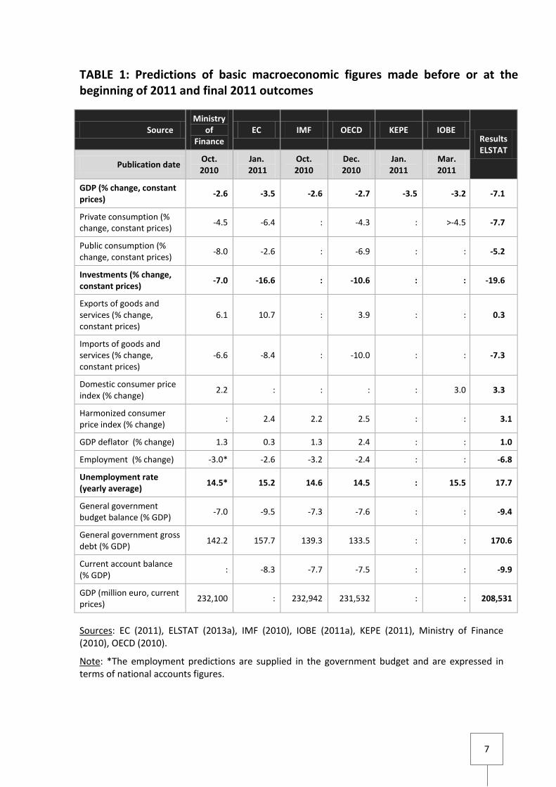
Table 1 lists the predictions made in late 2010 and early 2011 by the EC, IMF,

OECD, KEPE, IOBE, and the government about the evolution of basic

macroeconomic variables in the course of 2011, and (in the last column) the

corresponding final figures published by ELSTAT. It turns out that while the

5

predictions regarding the fall in real GDP were in the range of 2.6-3.5%, the

recession was much deeper: 7.1% (more than double the one predicted). In

looking into the factors behind the misprediction, we note that that though the

expected fall in private investments lied between 7.0 and 16.6%, the

contraction evidenced in the data was about 19.6%. The exports, which were

expected to grow by 3.9-10.7%, barely moved (+0.3%). The unemployment

rate, which was expected to lie between 14.5 and 15.5% rose to 17.7%.

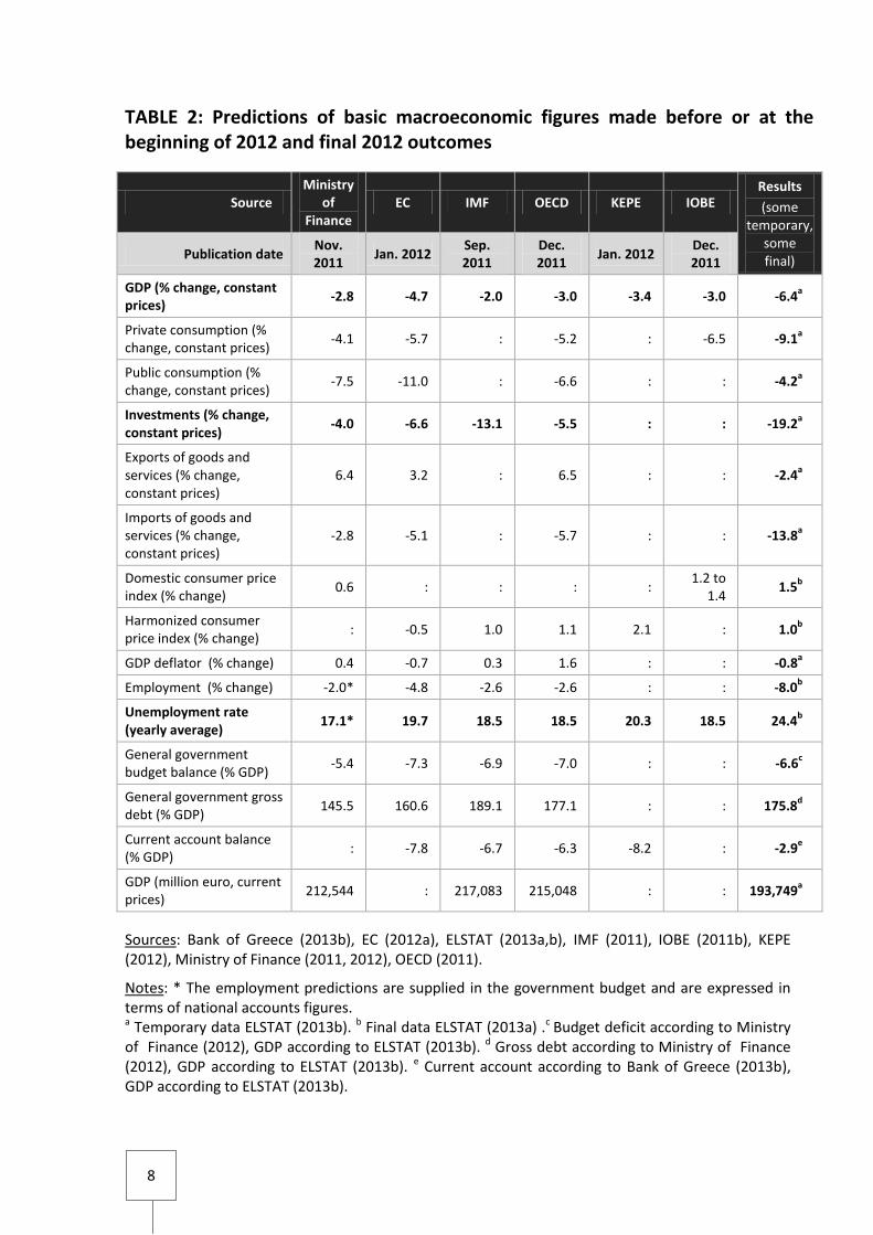
Likewise, even though the early predictions made about the fall in real GDP in

2012 were in the range of 2.0-4.7%, the estimates provided by ELSTAT (2013b)

suggest the recession was more severe: about 6.4%. (See Table 2.) Again, we

note that while the expectations regarding private investments lied between

-4.0 and -13.1%, the estimates provided by ELSTAT suggest that in fact private

investments shrunk considerably more: by about 19.6%. Imports, which were

expected to fall by 2.8-5.7%, and exports, which were expected to rise by 3.2%-

6.5% appear to have fallen by 13.8% and 2.4%, respectively. The

unemployment rate, which was expected to reach 17.1-20.3%, in the course of

the last quarter of 2012 seems to have reached 26.4% (as per ELSTAT’s

seasonally adjusted monthly data), thus affecting an annual average of 24.4%.

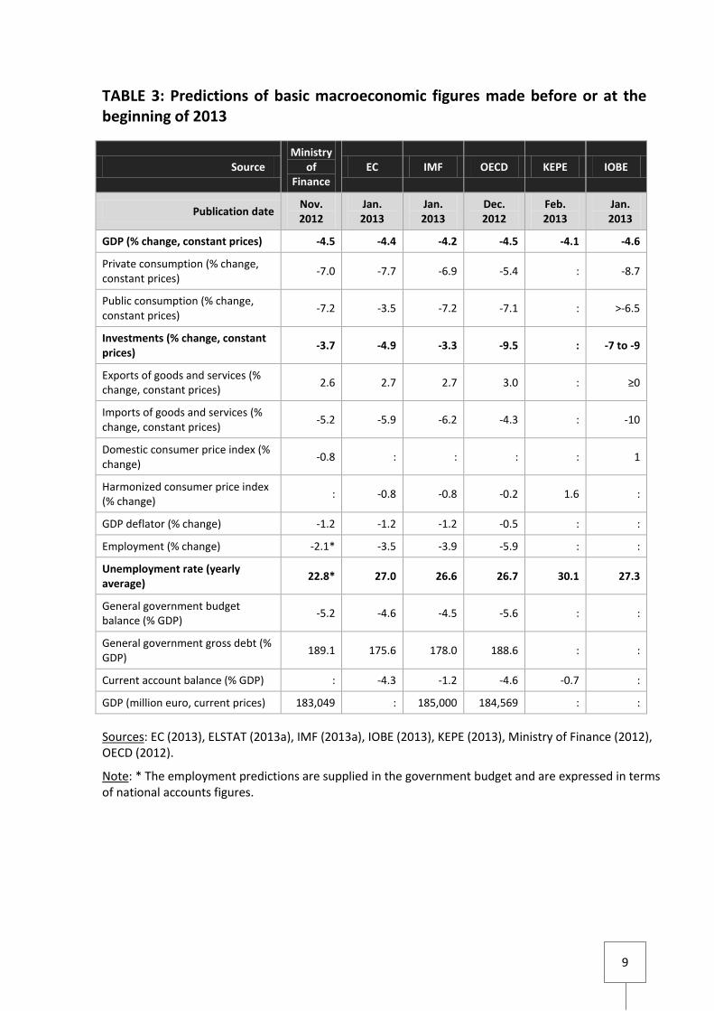
The early predictions made for 2013 prepare the public for a recession of 4.1-

4.6%, and come with expectations that private investments will fall by 3.3-

9.5%, and the unemployment rate will reach 22.8-27.3% (see Table 3). In some

quarters the figures foster optimism that the recession will be mild, about 3.0%

(Alpha Bank, 2013). On the other hand, KEPE expressed concern that the

unemployment rate may climb to 30.1%. In our view a rate in excess of 28% is

quite conceivable bearing in mind the rate’s continuous rise for the last couple

of years. The Bank of Greece (2013a: 21, 80) appears to share this view.

6

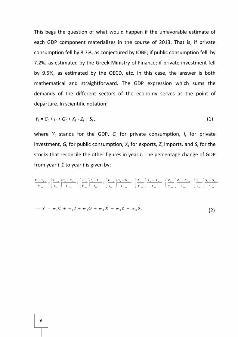
This begs the question of what would happen if the unfavorable estimate of

each GDP component materializes in the course of 2013. That is, if private

consumption fell by 8.7%, as conjectured by IOBE; if public consumption fell by

7.2%, as estimated by the Greek Ministry of Finance; if private investment fell

by 9.5%, as estimated by the OECD, etc. In this case, the answer is both

mathematical and straightforward. The GDP expression which sums the

demands of the different sectors of the economy serves as the point of

departure. In scientific notation:

Yt = Ct + It + Gt + Xt - Zt + St , (1)

where Yt stands for the GDP, Ct for private consumption, Ιt for private

investment, Gt for public consumption, Χt for exports, Ζt imports, and St for the

stocks that reconcile the other figures in year t. The percentage change of GDP

from year t-1 to year t is given by:

1 1 1 1 1 1 1 1 1 1 1 1 1

1 1 1 1 1 1 1 1 1 1 1 1 1

t t t t t t t t t t t t t t t t t t t t

t t t t t t t t t t t t t

Y Y C C C I I I G G G X X X Z Z Z S S S

Y Y C Y I Y G Y X Y Z Y S

1 2 3 4 5 6,Y w C w I w G w X w Z w S (2)

7

TABLE 1: Predictions of basic macroeconomic figures made before or at the beginning of 2011 and final 2011 outcomes

Source Ministry

of Finance

EC IMF OECD KEPE ΙΟΒΕ Results ELSTAT

Publication date Oct. 2010

Jan. 2011

Oct. 2010

Dec. 2010

Jan. 2011

Mar. 2011

GDP (% change, constant prices)

-2.6 -3.5 -2.6 -2.7 -3.5 -3.2 -7.1

Private consumption (% change, constant prices)

-4.5 -6.4 : -4.3 : >-4.5 -7.7

Public consumption (% change, constant prices)

-8.0 -2.6 : -6.9 : : -5.2

Investments (% change, constant prices)

-7.0 -16.6 : -10.6 : : -19.6

Exports of goods and services (% change, constant prices)

6.1 10.7 : 3.9 : : 0.3

Imports of goods and services (% change, constant prices)

-6.6 -8.4 : -10.0 : : -7.3

Domestic consumer price index (% change)

2.2 : : : : 3.0 3.3

Harmonized consumer price index (% change)

: 2.4 2.2 2.5 : : 3.1

GDP deflator (% change) 1.3 0.3 1.3 2.4 : : 1.0

Employment (% change) -3.0* -2.6 -3.2 -2.4 : : -6.8

Unemployment rate (yearly average)

14.5* 15.2 14.6 14.5 : 15.5 17.7

General government budget balance (% GDP)

-7.0 -9.5 -7.3 -7.6 : : -9.4

General government gross debt (% GDP)

142.2 157.7 139.3 133.5 : : 170.6

Current account balance (% GDP)

: -8.3 -7.7 -7.5 : : -9.9

GDP (million euro, current prices)

232,100 : 232,942 231,532 : : 208,531

Sources: EC (2011), ELSTAT (2013a), IMF (2010), IOBE (2011a), KEPE (2011), Ministry of Finance (2010), OECD (2010).

Note: *The employment predictions are supplied in the government budget and are expressed in terms of national accounts figures.

8

TABLE 2: Predictions of basic macroeconomic figures made before or at the beginning of 2012 and final 2012 outcomes

Source Ministry

of Finance

EC IMF OECD KEPE ΙΟΒΕ Results

(some temporary,

some final) Publication date

Nov. 2011

Jan. 2012 Sep. 2011

Dec. 2011

Jan. 2012 Dec. 2011

GDP (% change, constant prices)

-2.8 -4.7 -2.0 -3.0 -3.4 -3.0 -6.4a


-4.1 -5.7 : -5.2 : -6.5 -9.1a


-7.5 -11.0 : -6.6 : : -4.2a


-4.0 -6.6 -13.1 -5.5 : : -19.2a


6.4 3.2 : 6.5 : : -2.4a


-2.8 -5.1 : -5.7 : : -13.8a


0.6 : : : : 1.2 to

1.4 1.5

b


: -0.5 1.0 1.1 2.1 : 1.0b

GDP deflator (% change) 0.4 -0.7 0.3 1.6 : : -0.8a

Employment (% change) -2.0* -4.8 -2.6 -2.6 : : -8.0b


17.1* 19.7 18.5 18.5 20.3 18.5 24.4b


-5.4 -7.3 -6.9 -7.0 : : -6.6c


145.5 160.6 189.1 177.1 : : 175.8d

Current account balance (% GDP)

: -7.8 -6.7 -6.3 -8.2 : -2.9e

GDP (million euro, current prices)

212,544 : 217,083 215,048 : : 193,749a

Sources: Bank of Greece (2013b), EC (2012a), ELSTAT (2013a,b), IMF (2011), IOBE (2011b), KEPE (2012), Ministry of Finance (2011, 2012), OECD (2011).

Notes: * The employment predictions are supplied in the government budget and are expressed in terms of national accounts figures. a Temporary data ELSTAT (2013b). b Final data ELSTAT (2013a) .c Budget deficit according to Ministry of Finance (2012), GDP according to ELSTAT (2013b). d Gross debt according to Ministry of Finance (2012), GDP according to ELSTAT (2013b). e Current account according to Bank of Greece (2013b), GDP according to ELSTAT (2013b).

9

TABLE 3: Predictions of basic macroeconomic figures made before or at the beginning of 2013

Source Ministry

of Finance

EC IMF OECD KEPE ΙΟΒΕ

Publication date Nov. 2012

Jan. 2013

Jan. 2013

Dec. 2012

Feb. 2013

Jan. 2013

GDP (% change, constant prices) -4.5 -4.4 -4.2 -4.5 -4.1 -4.6


-7.0 -7.7 -6.9 -5.4 : -8.7


-7.2 -3.5 -7.2 -7.1 : >-6.5


-3.7 -4.9 -3.3 -9.5 : -7 to -9


2.6 2.7 2.7 3.0 : ≥0


-5.2 -5.9 -6.2 -4.3 : -10


-0.8 : : : : 1


: -0.8 -0.8 -0.2 1.6 :

GDP deflator (% change) -1.2 -1.2 -1.2 -0.5 : :

Employment (% change) -2.1* -3.5 -3.9 -5.9 : :


22.8* 27.0 26.6 26.7 30.1 27.3


-5.2 -4.6 -4.5 -5.6 : :


189.1 175.6 178.0 188.6 : :

Current account balance (% GDP) : -4.3 -1.2 -4.6 -0.7 :

GDP (million euro, current prices) 183,049 : 185,000 184,569 : :

Sources: EC (2013), ELSTAT (2013a), IMF (2013a), IOBE (2013), KEPE (2013), Ministry of Finance (2012), OECD (2012).

Note: * The employment predictions are supplied in the government budget and are expressed in terms of national accounts figures.

10

TABLE 4: Relative weights of the expenditure components in real GDP (%)

Year Private

consumption (w1)

Public consumption

(w2)

Private investments

(w3)

Exports of goods and

services (w4)

Imports of goods and

services (w5)

Change in stocks (w6)

2000 69.06 19.68 20.94 24.96 -37.00 2.36

2001 69.57 19.03 21.07 23.95 -35.92 2.30

2002 70.45 19.72 22.30 21.21 -34.29 0.61

2003 68.67 18.45 23.54 20.60 -33.33 2.05

2004 68.32 18.30 22.64 23.16 -33.74 1.32

2005 69.79 18.10 20.73 23.21 -32.50 0.67

2006 69.02 17.68 22.58 22.95 -34.22 1.99

2007 69.06 18.29 26.78 23.74 -37.85 -0.02

2008 72.16 17.85 22.99 24.19 -38.27 1.09

2009 73.33 19.33 20.48 20.12 -31.52 -1.73

2010 72.32 18.57 18.31 22.26 -31.12 -0.35

2011 71.84 18.96 15.84 24.05 -31.04 0.34

2012 69.78 19.40 13.67 25.06 -28.59 0.68

Note: Calculations based on quarterly data of GDP and its expenditure components as published by ELSTAT (2013b) until the last quarter of 2012.

TABLE 5: Estimates of three international organizations and of the Greek government about the evolution in 2013 of real GDP based on predictions regarding the expenditure components

Source Ministry

of Finance EC IMF OECD

Publication date Oct. 2012 Jan. 2013 Jan. 2013 Dec. 2012

Real GDP estimate (% change) (calculations based on items 1-6 and the 2012 weights wi of Table 4)

-4.65 -4.36 -4.21 -4.46

Published prediction of real GDP (% change) -4.5 -4.4 -4.2 -4.5

1. Private consumption (Ċ) -7.0 -7.7 -6.9 -5.4

2. Public consumption (Ġ) -7.2 -3.5 -7.2 -7.1

3. Investments (İ) -3.7 -4.9 -3.3 -9.5

4. Exports of goods and services (Ẋ) 2.6 2.7 2.7 3.0

5. Imports of goods and services (Ż) -5.2 -5.9 -6.2 -4.3

6. Change in stocks (Ṡ) * 0.0 0.0 *

Note: * Since the Ministry of Finance and OECD have not published their estimates concerning the change in stocks this was taken as equal to zero for the calculations of real GDP, as in the EC and IMF predictions.

11

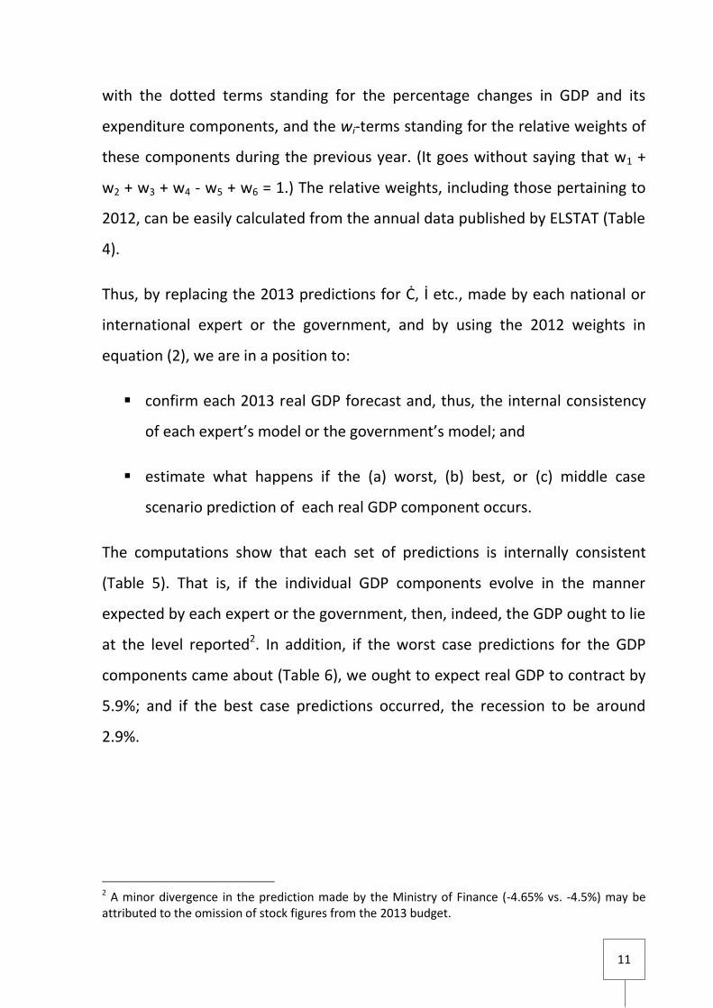
with the dotted terms standing for the percentage changes in GDP and its

expenditure components, and the wi-terms standing for the relative weights of

these components during the previous year. (It goes without saying that w1 +

w2 + w3 + w4 - w5 + w6 = 1.) The relative weights, including those pertaining to

2012, can be easily calculated from the annual data published by ELSTAT (Table

4).

Thus, by replacing the 2013 predictions for Ċ, İ etc., made by each national or

international expert or the government, and by using the 2012 weights in

equation (2), we are in a position to:

confirm each 2013 real GDP forecast and, thus, the internal consistency

of each expert’s model or the government’s model; and

estimate what happens if the (a) worst, (b) best, or (c) middle case

scenario prediction of each real GDP component occurs.

The computations show that each set of predictions is internally consistent

(Table 5). That is, if the individual GDP components evolve in the manner

expected by each expert or the government, then, indeed, the GDP ought to lie

at the level reported2. In addition, if the worst case predictions for the GDP

components came about (Table 6), we ought to expect real GDP to contract by

5.9%; and if the best case predictions occurred, the recession to be around

2.9%.

2 A minor divergence in the prediction made by the Ministry of Finance (-4.65% vs. -4.5%) may be attributed to the omission of stock figures from the 2013 budget.

12

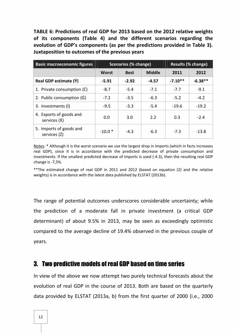
TABLE 6: Predictions of real GDP for 2013 based on the 2012 relative weights of its components (Table 4) and the different scenarios regarding the evolution of GDP’s components (as per the predictions provided in Table 3). Juxtaposition to outcomes of the previous years

Basic macroeconomic figures Scenarios (% change) Results (% change)

Worst Best Middle 2011 2012

Real GDP estimate (Ẏ) -5.91 -2.92 -4.57 -7.10** -6.38**

1. Private consumption (Ċ) -8.7 -5.4 -7.1 -7.7 -9.1

2. Public consumption (Ġ) -7.2 -3.5 -6.3 -5.2 -4.2

3. Investments (İ) -9.5 -3.3 -5.4 -19.6 -19.2

4. Exports of goods and services (Ẋ)

0.0 3.0 2.2 0.3 -2.4

5. Imports of goods and services (Ż)

-10.0 * -4.3 -6.3 -7.3 -13.8

Notes: * Although it is the worst scenario we use the largest drop in imports (which in facts increases real GDP), since it is in accordance with the predicted decrease of private consumption and investments. If the smallest predicted decrease of imports is used (-4.3), then the resulting real GDP change is -7,5%.

**The estimated change of real GDP in 2011 and 2012 (based on equation (2) and the relative weights) is in accordance with the latest data published by ELSTAT (2013b).

The range of potential outcomes underscores considerable uncertainty; while

the prediction of a moderate fall in private investment (a critical GDP

determinant) of about 9.5% in 2013, may be seen as exceedingly optimistic

compared to the average decline of 19.4% observed in the previous couple of

years.

3. Two predictive models of real GDP based on time series

In view of the above we now attempt two purely technical forecasts about the

evolution of real GDP in the course of 2013. Both are based on the quarterly

data provided by ELSTAT (2013a, b) from the first quarter of 2000 (i.e., 2000

13

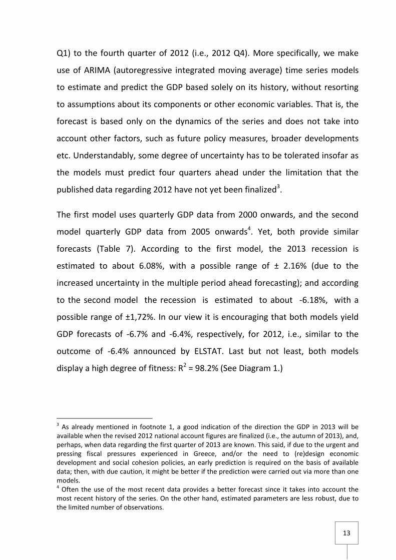
Q1) to the fourth quarter of 2012 (i.e., 2012 Q4). More specifically, we make

use of ARIMA (autoregressive integrated moving average) time series models

to estimate and predict the GDP based solely on its history, without resorting

to assumptions about its components or other economic variables. That is, the

forecast is based only on the dynamics of the series and does not take into

account other factors, such as future policy measures, broader developments

etc. Understandably, some degree of uncertainty has to be tolerated insofar as

the models must predict four quarters ahead under the limitation that the

published data regarding 2012 have not yet been finalized3.

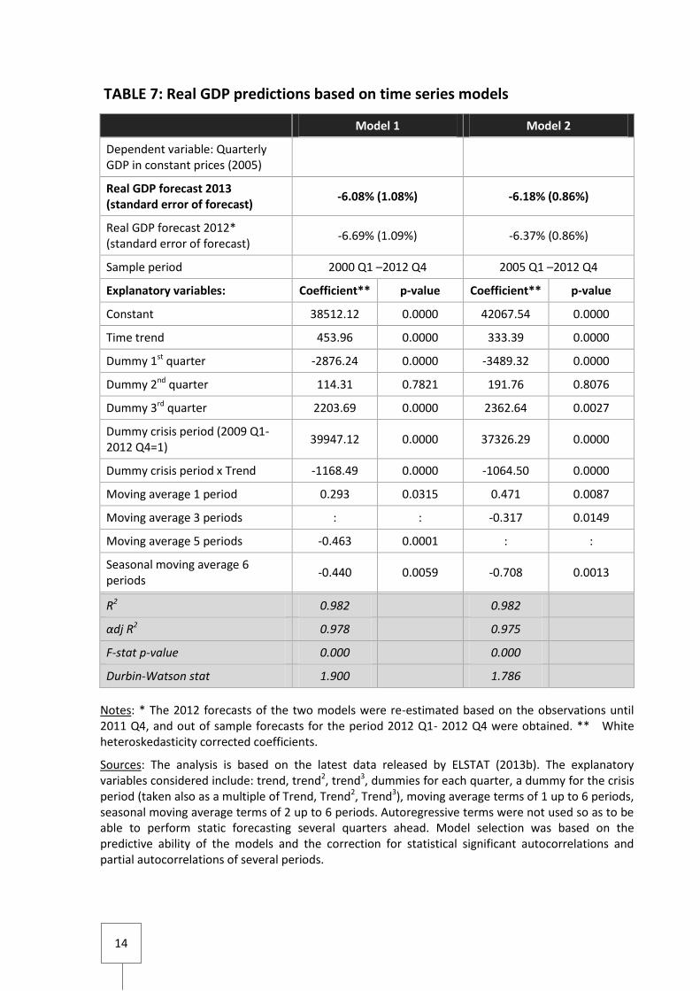
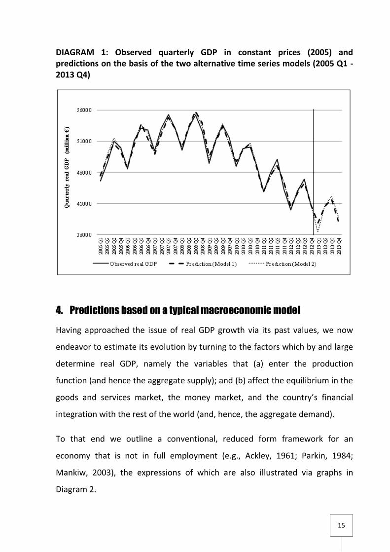
The first model uses quarterly GDP data from 2000 onwards, and the second

model quarterly GDP data from 2005 onwards4. Yet, both provide similar

forecasts (Table 7). According to the first model, the 2013 recession is

estimated to about 6.08%, with a possible range of ± 2.16% (due to the

increased uncertainty in the multiple period ahead forecasting); and according

to the second model the recession is estimated to about -6.18%, with a

possible range of ±1,72%. In our view it is encouraging that both models yield

GDP forecasts of -6.7% and -6.4%, respectively, for 2012, i.e., similar to the

outcome of -6.4% announced by ELSTAT. Last but not least, both models

display a high degree of fitness: R2 = 98.2% (See Diagram 1.)

3 As already mentioned in footnote 1, a good indication of the direction the GDP in 2013 will be available when the revised 2012 national account figures are finalized (i.e., the autumn of 2013), and, perhaps, when data regarding the first quarter of 2013 are known. This said, if due to the urgent and pressing fiscal pressures experienced in Greece, and/or the need to (re)design economic development and social cohesion policies, an early prediction is required on the basis of available data; then, with due caution, it might be better if the prediction were carried out via more than one models. 4 Often the use of the most recent data provides a better forecast since it takes into account the most recent history of the series. On the other hand, estimated parameters are less robust, due to the limited number of observations.

14

TABLE 7: Real GDP predictions based on time series models

Model 1 Model 2

Dependent variable: Quarterly GDP in constant prices (2005)

Real GDP forecast 2013 (standard error of forecast)

-6.08% (1.08%) -6.18% (0.86%)

Real GDP forecast 2012* (standard error of forecast)

-6.69% (1.09%) -6.37% (0.86%)

Sample period 2000 Q1 –2012 Q4 2005 Q1 –2012 Q4

Explanatory variables: Coefficient** p-value Coefficient** p-value

Constant 38512.12 0.0000 42067.54 0.0000

Time trend 453.96 0.0000 333.39 0.0000

Dummy 1st quarter -2876.24 0.0000 -3489.32 0.0000

Dummy 2nd quarter 114.31 0.7821 191.76 0.8076

Dummy 3rd quarter 2203.69 0.0000 2362.64 0.0027

Dummy crisis period (2009 Q1-2012 Q4=1)

39947.12 0.0000 37326.29 0.0000

Dummy crisis period x Trend -1168.49 0.0000 -1064.50 0.0000

Moving average 1 period 0.293 0.0315 0.471 0.0087

Moving average 3 periods : : -0.317 0.0149

Moving average 5 periods -0.463 0.0001 : :

Seasonal moving average 6 periods

-0.440 0.0059 -0.708 0.0013

R2 0.982

0.982

αdj R2 0.978

0.975

F-stat p-value 0.000

0.000

Durbin-Watson stat 1.900

1.786

Notes: * The 2012 forecasts of the two models were re-estimated based on the observations until 2011 Q4, and out of sample forecasts for the period 2012 Q1- 2012 Q4 were obtained. ** White heteroskedasticity corrected coefficients.

Sources: The analysis is based on the latest data released by ELSTAT (2013b). The explanatory variables considered include: trend, trend2, trend3, dummies for each quarter, a dummy for the crisis period (taken also as a multiple of Trend, Trend2, Trend3), moving average terms of 1 up to 6 periods, seasonal moving average terms of 2 up to 6 periods. Autoregressive terms were not used so as to be able to perform static forecasting several quarters ahead. Model selection was based on the predictive ability of the models and the correction for statistical significant autocorrelations and partial autocorrelations of several periods.

15

DIAGRAM 1: Observed quarterly GDP in constant prices (2005) and predictions on the basis of the two alternative time series models (2005 Q1 - 2013 Q4)

4. Predictions based on a typical macroeconomic model

Having approached the issue of real GDP growth via its past values, we now

endeavor to estimate its evolution by turning to the factors which by and large

determine real GDP, namely the variables that (a) enter the production

function (and hence the aggregate supply); and (b) affect the equilibrium in the

goods and services market, the money market, and the country’s financial

integration with the rest of the world (and, hence, the aggregate demand).

To that end we outline a conventional, reduced form framework for an

economy that is not in full employment (e.g., Ackley, 1961; Parkin, 1984;

Mankiw, 2003), the expressions of which are also illustrated via graphs in

Diagram 2.

16

The equilibrium in the money market is given by:

r=f(M, Y, P, constant terms), (3)

where r stands for the interest rate, Μ the quantity of money, Υ the real GDP, P

the average price level.

The equilibrium in the goods and services market is given by:

r=g(Υ, G, Β, I1, Y*, P, constant terms), (4)

where G stands for public expenses, Β for transfers, I1 for private investments

attributed to expectations over the future level of Y, Υ* for the income of

foreign trading partners (in this context: the total GDP of OECD countries).

Typically, indirect taxes are also included, but here by and large replicate the

time series of Υ.

At the same time the financial integration with respect to the rest of the world

is given by:

r=h(Y, Y*, P, constant terms) (5)

under flexible exchange rates. However, r is inflexible in the case of fixed

exchange rates.

So, the Aggregate Demand is derived on the basis of the expressions (3)-(5):

P=j(Y, M1, G, Β, I1, Y*, constant terms). (6)

In addition, the Aggregate Supply is given by:

P=ω(L, K, Α, constant terms), (7)

where L stands for the number of people employed in paid work activities, Κ for

the capital stock, Α for entrepreneurship and technology. The amount of land is

taken as constant.

17

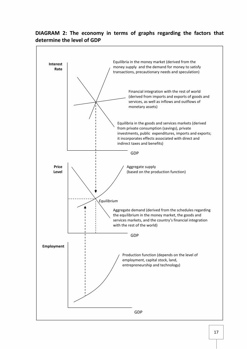
DIAGRAM 2: The economy in terms of graphs regarding the factors that determine the level of GDP

*

Equilibrium

Equilibria in the money market (derived from the money supply and the demand for money to satisfy transactions, precautionary needs and speculation)

Financial integration with the rest of world (derived from imports and exports of goods and services, as well as inflows and outflows of monetary assets)

Equilibria in the goods and services markets (derived from private consumption (savings), private investments, public expenditures, imports and exports; it incorporates effects associated with direct and indirect taxes and benefits)

GDP

Aggregate supply (based on the production function)

Aggregate demand (derived from the schedules regarding the equilibrium in the money market, the goods and services markets, and the country’s financial integration with the rest of the world)

Production function (depends on the level of employment, capital stock, land, entrepreneurship and technology)

GDP

GDP

Employment

Price Level

Interest Rate

18

So based on equations (6) and (7), the real GDP level may be written as follows:

Υ=y( M, G, Β, I1, Y*, L, K, Α, constant terms). (8)

In order to empirically estimate and predict the real GDP level we consider the

time series of the (a) annual 1960-2011 national accounts published by ELSTAT;

(b) monthly 1980-2012 monetary aggregates supplied by the Bank of Greece

(2013b); (c) annual 1988-2001 drachma to US dollar and 2002-2013 euro to US

dollar exchange rates, and (d) annual 1960-2012 five-year government bond

yields supplied by Eurostat (2013). Then, after testing the interpretive ability of

these regressors and taking into account the currency changeover, and

weighing up the need to preserve degrees of freedom5, we estimate the

following variant of equation (8) for the 1981-2011 period:

Change in real GDP1981-2011 = 0.027*ΔL + 0.639*ΔΙ1, N=31, R2=43.39%, (9) (3‰) (2‰)

with ΔL standing for the annual change in the number of actively employed

people, and ΔΙ1 for the annual change in the value of private investments

attributed to expectations over future income and demand (in billion euro at

constant 2005 prices)6. The aforementioned regressors prevail over other

available explanatory variables. The estimated coefficients, obtained via a

robust variance estimator, are statistically significant. (The probabilities of error

(p-values) are supplied in parentheses below the estimates.)

5 Understandably due to the paucity of observations (32-52 years) we do not use many explanatory variables. Among those considered is the technology-entrepreneurship vector supplied in Diagram 4.III. It is empirically estimated (as a residual) from the production function Υ = L0.567k0.942 recovered from the 1960-2011 data. (k is the orthogonal variant (residual) of capital with respect to labor, L. R2=99.54%. The estimated output elasticities of labor and capital are statistically significant at the 1‰ level.) A more detailed estimate of the technology-entrepreneurship variable across regions in Greece has been carried out by KEPE (2010). 6 The size of I1 is empirically estimated from the residuals of Ι1960-2011 = 6.455 – 0.420*r + 0.198*Y. R2=90.68%. The coefficients are statistically significant at the 1‰ level.

19

It goes without saying that it is important to verify the equation’s predictive

capacity for 2012. Indeed, for an employment (job market) contraction of

about 371 thousand people and a private investment contraction of about 5.5

billion euro (as per the 2012 national account figures published by ELSTAT)7,

according to expression (9) we should expect a fall in real GDP of about 6.6%.

According to the official statistics, indeed, in 2012 the contraction was about

that. (See Table 2.)

Likewise, in order to engage in predictions for 2013, we incorporate the figures

pertaining to 2012, and re-estimate the relationship. It turns out that:

Change in real GDP1981-2012 = 0.026*ΔL + 0.666*ΔΙ1, N=32, R2=50.91% (10) (<1‰) (2‰)

So for an additional contraction in employment of about 250-300 thousand

people (i.e., a contraction smaller than the one observed in 2012)8, and private

investment of 4.7 billion euro (i.e., four fifths of the one observed in 2012),

ceteris paribus, real GDP is estimated to shrink by 5.6-6.4%9. More if the

contraction in employment in larger. See Table 8. This is consistent with (and

by and large corroborates) the findings of the two technical predictions. On the

other hand, if in the course of 2013, private investment falls as much as in the

7 The 5.5 billion contraction in private investments corresponds to the 19.2% drop which is supplied in the last column of Table 2. 8 If these people do not migrate or withdraw from the workforce then the unemployment rate will climb to 28-29%. 9 If we incorporate the figures associated with 2012, then the investment expression takes the form: Ι = 6.329 – 0.377*r + 0.192*Y. R2=87.15%. The estimated coefficients are statistically significant at the 1‰ level. Accordingly, Ι1 is estimated from the residuals as follows: Ι1 = Ι - (6.329 – 0.377*r + 0.192*Y), hence ΔΙ1 = ΔΙ + 0.377*Δr – 0.192*ΔY. As a consequence, the 2013 GDP prediction is calculated in conjunction with expression (10) and is a follows: ΔΥ = 0.026*ΔL + 0.666*ΔΙ1 = 0.026*ΔL + 0.666* (ΔΙ + 0.377*Δr – 0.192*ΔY) → ΔΥ = (0.026*ΔL + 0.666* ΔΙ + 0.251*Δr) / (1.128). To estimate the change in real GDP all one has to do is to substitute the values of ΔL, ΔΙ, Δr. See Table 8.

20

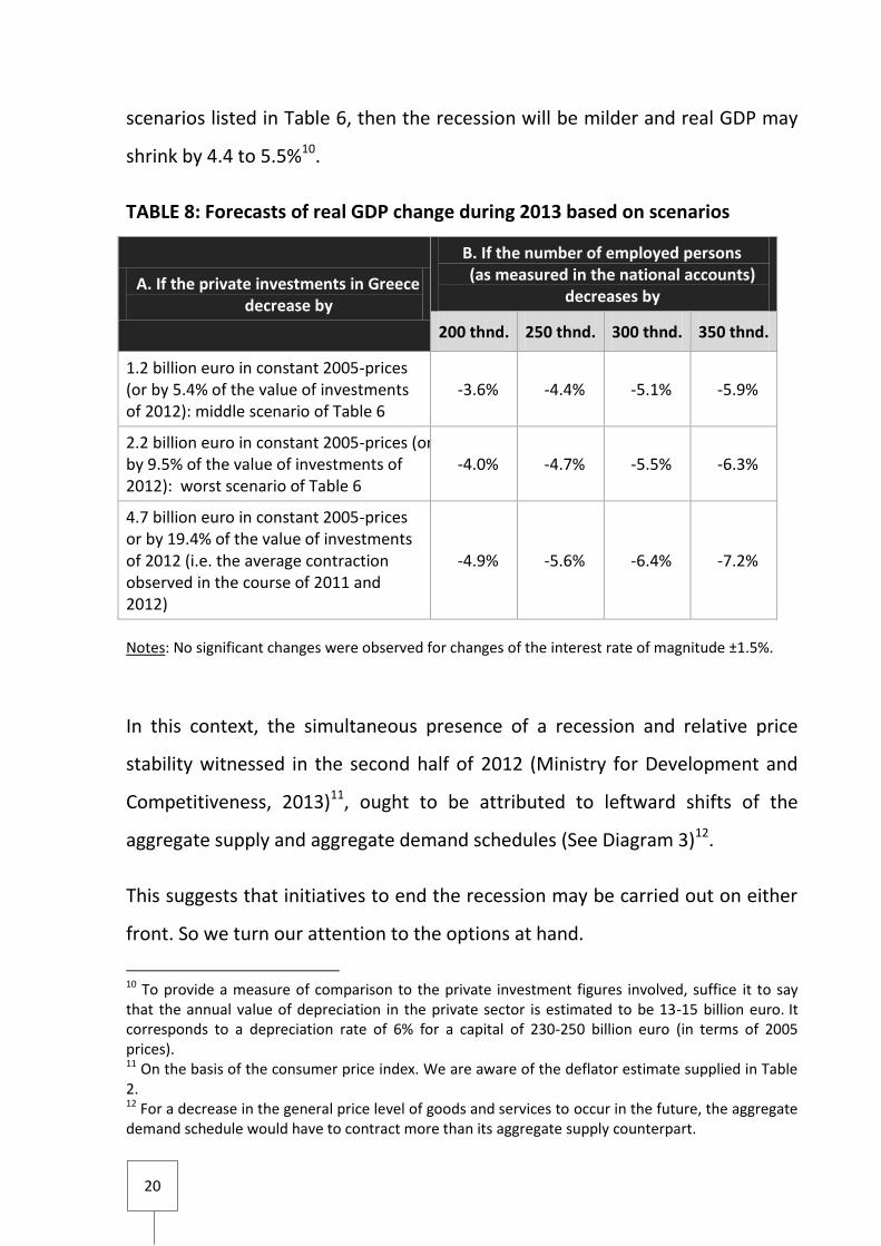
scenarios listed in Table 6, then the recession will be milder and real GDP may

shrink by 4.4 to 5.5%10.

TABLE 8: Forecasts of real GDP change during 2013 based on scenarios

A. If the private investments in Greece decrease by

Β. If the number of employed persons (as measured in the national accounts)

decreases by

200 thnd. 250 thnd. 300 thnd. 350 thnd.

1.2 billion euro in constant 2005-prices (or by 5.4% of the value of investments of 2012): middle scenario of Table 6

-3.6% -4.4% -5.1% -5.9%

2.2 billion euro in constant 2005-prices (or by 9.5% of the value of investments of 2012): worst scenario of Table 6

-4.0% -4.7% -5.5% -6.3%

4.7 billion euro in constant 2005-prices or by 19.4% of the value of investments of 2012 (i.e. the average contraction observed in the course of 2011 and 2012)

-4.9% -5.6% -6.4% -7.2%

Notes: No significant changes were observed for changes of the interest rate of magnitude ±1.5%.

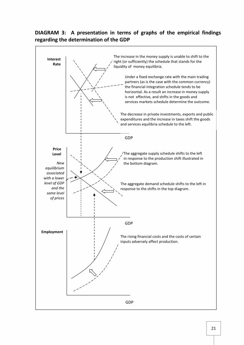
In this context, the simultaneous presence of a recession and relative price

stability witnessed in the second half of 2012 (Ministry for Development and

Competitiveness, 2013)11, ought to be attributed to leftward shifts of the

aggregate supply and aggregate demand schedules (See Diagram 3)12.

This suggests that initiatives to end the recession may be carried out on either

front. So we turn our attention to the options at hand.

10 To provide a measure of comparison to the private investment figures involved, suffice it to say that the annual value of depreciation in the private sector is estimated to be 13-15 billion euro. It corresponds to a depreciation rate of 6% for a capital of 230-250 billion euro (in terms of 2005 prices). 11 On the basis of the consumer price index. We are aware of the deflator estimate supplied in Table 2. 12 For a decrease in the general price level of goods and services to occur in the future, the aggregate demand schedule would have to contract more than its aggregate supply counterpart.

21

DIAGRAM 3: A presentation in terms of graphs of the empirical findings regarding the determination of the GDP

Interest Rate

The increase in the money supply is unable to shift to the right (or sufficiently) the schedule that stands for the liquidity of money equilibria.

Employment

Price Level

Under a fixed exchange rate with the main trading partners (as is the case with the common currency) the financial integration schedule tends to be horizontal. As a result an increase in money supply is not effective, and shifts in the goods and services markets schedule determine the outcome.

The decrease in private investments, exports and public expenditures and the increase in taxes shift the goods and services equilibria schedule to the left.

GDP

GDP

GDP

The aggregate supply schedule shifts to the left in response to the production shift illustrated in the bottom diagram.

The aggregate demand schedule shifts to the left in response to the shifts in the top diagram.

New equilibrium associated

with a lower level of GDP

and the same level

of prices

The rising financial costs and the costs of certain inputs adversely affect production.

22

5. Some options

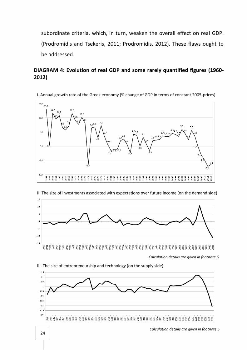
First of all we ought to take into account that the current economic crisis is the

longest and most severe the country has experienced in the last sixty years (see

Diagram 4.I). The closest historical parallel may be found in 1974, a year

marked by political instability and regional tension as the Turkish invasion of

Cyprus brought Greece to the brink of war with Turkey. However, the similarity

is superficial. In economic terms, the current situation is clearly worse both in

magnitude and length (five consecutive years, not counting 2013). Last but not

least, whereas (up until recently) it was possible to deal with negative growth

rates by resorting to tried, tested and effective fiscal and monetary

interventions, as mentioned in the Introduction, these basic policy instruments

are no longer at the government's disposal. As a result, the options are limited.

Like:

a) Encourage foreign demand for Greek products and services, and attract

investments in all sorts of projects (whether above or under the ground or

water, whether tangible or intangible assets). An improved economic climate

in the euro-zone and/or worldwide may be helpful13. Yet, the effort should

be made even if conditions abroad became unfavorable or the creditability

of other EU member-states were downgraded, confidence in the security of

deposits in the euro-zone at large undermined etc14. Unfortunately the

13 Our econometric analyses of macroeconomic (national account) figures suggest that ceteris paribus: An increase (decrease) in incomes by 1% in OECD-countries will positively (negatively) affect Greek exports by 0.55%. A decrease (increase) by 1% of relative prices in Greece vis-à-vis OECD countries is expected to stimulate (reduce) the volume of tourism services from foreign countries by 0.87%. A decrease (increase) in the real effective exchange rate by 1% is expected to stimulate (reduce) Greek exports by 0.32%. 14 For instance, the EC-ECB-IMF proposition in mid-March to seize a part of insured deposits in Cyprus (though eventually rejected by the Cypriot legislature) and a large portion of deposits over 100,000 euro, is likely to prevent potential investors from engaging in businesses (for which this kind of large bank account are needed) in other euro-zone countries in which the EC, the ECB and the IMF collectively have a say.

23

euphoria of 2007-2008 about the country’s prospects has been succeeded by

disappointment (see Diagram 4.II). For the psychology to change a

succession of consistent signals by the authorities and the public that build

faith in doing business in Greece is needed. May the long-awaited

resumption of work on the expansion and modernization of the

transportation network, privatizations, and the achievement of a budget

surplus be in that direction.

b) Increase the quantity and/or velocity of money in order to reduce the cost of

borrowing and facilitate monetary transactions. This may be advanced in a

number of ways: By recapitalizing the banking sector, by enabling the state

to pay the money owed to private sector suppliers and VAT returns to other

businesses, by deregulating Sunday shopping among small retailers etc.

c) Deregulate markets and remove distortions in competition (in agriculture,

trade, services, everywhere) so as to reduce prices and raise the level of

output.

d) Promote the overall state of technology and entrepreneurship, a pair of

essential production inputs which currently seem to be at an all-time low

(see Diagram 4.ΙΙΙ); and set up a friendlier business environment (see Vima,

2011).

e) Absorb and utilize the funds earmarked for economic development by the

EU via the Greek National Strategic Reference Framework (NSRF), in areas

and sectors associated with significant multipliers. Unfortunately, several

NSRF operational programs lack a strategic focus, while planning and

implementation are often based on (i) broad regional averages with little or

no consideration for intra-regional heterogeneity and spillovers or (ii)

24

subordinate criteria, which, in turn, weaken the overall effect on real GDP.

(Prodromidis and Tsekeris, 2011; Prodromidis, 2012). These flaws ought to

be addressed.

DIAGRAM 4: Evolution of real GDP and some rarely quantified figures (1960-2012)

Ι. Annual growth rate of the Greek economy (% change of GDP in terms of constant 2005-prices)

Calculation details are given in footnote 6

Calculation details are given in footnote 5

ΙΙ. The size of investments associated with expectations over future income (on the demand side)

ΙΙΙ. The size of entrepreneurship and technology (on the supply side)

25

6. Conclusions

The early estimates of a number of international organizations, the Greek

government, and the country’s research institutes in 2011 and 2012, suggested

the recession would range between 2.6-3.5% and 2.0-4.7%, respectively, when

in fact real GDP decreased by 7.1% in 2011, and 6.4% in 2012 (according the

temporary data of ELSTAT (2013b)). Similar forecast errors are observed for

individual GDP components. Insofar as the early 2013 estimates provided by

these institutes and the government point in the direction of a 4.2-4.6%

recession, we are concerned that they may be overly optimistic as well. Maybe

it is better if we treated these projections with caution.

According to alternative models which we estimate based on different

methodological approaches and temporal frequency, we find that any

prediction for the actual GDP growth contains a high degree of uncertainty. The

recession can lie in the range of 2.9-7.2%, possibly 4.4-6.4%, if the

unemployment rate climbs to 28-30%. So it is best to avoid any complacency

and to keep on taking steps towards improving the variables which contribute

to growth as if the likelihood of last year's recession has not gone away. The

situation is sensitive and stabilization has not yet occurred. As much as we all

hope for the best, and that the measures taken by the policy-makers and the

mobilization of society at large may halt the downward economic trend of

recent years and even disprove the contractionary economic forecasts, it is

important to have (prepare) alternative or additional plans in the direction of

economic development, financial and social cohesion if the optimistic scenarios

do not materialize.

As the above lines were printed, ELSTAT announced a smaller the expected

decline in real GDP during the second quarter of 2013: Specifically, that the

26

5,6% drop in the first quarter (vis- à-vis the respective quarter of 2012) was

succeeded by 3,8% drop in the second quarter. Beyond illustrating our basic

point regarding the uncertainty of early projections, coupled with a general

impression that the tourist season went exceptionally well in the third quarter

(thus hindering a rise in unemployment), this may be a sign that the economy is

inching toward the lower end of the estimated range provided above. The

argument regarding complacency holds.

27

References

Ackley G. (1961). Macroeconomic Theory. New York: Macmillan.

Alogoskoufis G. (2012). Greece’s Sovereign Debt Crisis: Retrospect and Prospect. LSE Hellenic Observatory Paper on Greece and Southeast Europe, 54.

Alpha Bank (2013). Weekly Economic Report. February 28th. [In Greek.] Athens: Division of Economic-Market Research.

Andreou E., E. Ghysels and A. Kourtellos A. (2013). “Should Macroeconomic Forecasters Use Daily Financial Data and How?” Journal of Business & Economic Statistics, 31: 240-251.

Antipa P., K. Barhoumi, V. Brunhes-Lesage and O. Darne (2012). “Nowcasting German GDP: A comparison of bridge and factor models.” Journal of Policy Modeling, 34: 864-878.

Bank of Greece (2013a). Report of the Board Director for the year 2012. [In Greek.] Athens.

Bank of Greece (2013b). Data accessed via www.bankofgreece.gr during the last week of February and the first week of March 2013.

Blanchard O. and D. Leigh (2013). Growth Forecast Errors and Fiscal Multipliers. IMF Working Paper, 13/1.

Barhoumi K., O. Darne, L. Ferrara and B. Pluyaud (2012). “Monthly GDP Forecasting using Bridge Models: Application for the French Economy.” Bulletin of Economic Research, 64 Issue Supplement: s53-s70.

Buettner T and B. Kauder (2010). “Revenue Forecasting Practices: Differences across Countries and Consequences for Forecasting Performance.” Fiscal Studies, 31: 313-340.

Cushman D.O. (2012). “Mankiw vs. DeLong and Krugman on the CEA’s Real GDP Forecasts in Early 2009: What Might a Time Series Econometrician Have Said?” Econ Journal Watch, 9: 309-349.

EC (2006). Regulation No 1083/2006 laying down general provisions on the European Regional Development Fund, the European Social Fund and the Cohesion Fund and repealing Regulation (EC) No 1260/1999. Luxembourg: Publications Office of the European Union.

EC (2011). Εuropean economic forecast spring 2011. Brussels: Directorate-General for Economic and Financial Affairs of the European Commission.

28

EC (2012a). Εuropean economic forecast spring 2012. Brussels: Directorate-General for Economic and Financial Affairs of the European Commission.

ELSTAT (2013a). Data accessed via www.statistics.gr during the last week of February and the first week of March 2013.

ELSTAT (2013b). Press release of March 11th. [In Greek.] Piraeus.

Εurostat (2013). Statistical data retrieved from Eurostat epp.eurostat.ec.europa.eu during the last week of February and first week of March 2013.

Ferrara L. and C. Marsilli (2013). “Financial variables as leading indicators of GDP growth: Evidence from a MIDAS approach during the Great Recession.” Applied Economic Letters, 20: 233-237.

Heilemann U. and H. Stekler (2007). “Introduction to ‘The future of macroeconomic forecasting’.” International Journal of Forecasting, 23: 159-165

IMF (2010). IMF World Economic Outlook. October. Washington DC.

IMF (2011). IMF World Economic Outlook. September. Washington DC.

IMF (2013a). Greece. IMF Country Report No. 13/20. January. Washington DC.

IMF (2013b). IMF Country Report No. 13/156. June. Washington DC.

IOBE (2011a). The Greek Economy 1/11. Quarterly Bulletin No. 63. [In Greek.] Athens.

ΙΟΒΕ (2011b). The Greek Economy 4/11. Quarterly Bulletin No. 66. [In Greek.] Athens.

ΙΟΒΕ (2013). The Greek Economy 4/12. Quarterly Bulletin No. 70. [In Greek.] Athens.

Jonung L. and M. Larch (2006). Fiscal policy in the EU: Are official output forecasts biased? Economic Policy, 21: 491-534.

KEPE (2010). The regional dimension of the National Strategic Reference Framework. [In Greek.] Prepared in two volumes by P. Prodromidis, Th. Tsekeris, J. Anastasakou, L. Athanassiou, N. Kanellopoulos, R. Karagianni, A. Petralias, I. Psycharis, S. Spathi, T. Terrovitis, K. Vogiatzoglou. Athens.

KEPE (2011). The short-term predictions. Press release of January 19th. [In Greek.] Athens.

KEPE (2012). The short-term predictions for the basic macroeconomic figures of the Greek economy. Press release of January 31st. [In Greek.] Athens.

KEPE (2013). Predictions for the short-term perspectives of the macroeconomic figures of the Greek economy. Press release of February 14th. [In Greek.] Athens.

http://www.statistics.gr/

29

Kiriakidis M. and A. Kargas (2013). “Greek GDP forecast estimates.” Applied Economic Letters. 20: 767-772.

Loungani P. (2001). “How accurate are private sector forecasts? Cross-country evidence from consensus forecasts of output growth.” International Journal of Forecasting, 17: 419-432.

Mankiw N.G. (2003). Macroeconomics. New York: Worth.

Merola R. and J.J. Pérez (2012). Fiscal forecast errors: Governments vs independent agencies? Documentos de Trabajo No 1233. Madrid: Banco de España.

Ministry for Development and Competitiveness (2013). The Greek market is getting cheaper. The evolution of prices during 2012. [In Greek.] Athens.

Ministry of Finance (2010). Government budget 2011. [In Greek.] Athens.



OECD (2010). OECD Economic Outlook , 88. Paris.

OECD (2011). OECD Economic Outlook , 90. Paris.

OECD (2012). OECD Economic Outlook, 92. Paris.

Öller L.E. and B. Barot (2000). “The accuracy of European growth and inflation forecasts.” International Journal of Forecasting, 16: 293-315.

Parkin M. (1984). Macroeconomics. Englewood Cliffs, NJ: Prentice-Hall.

Pisani-Ferry J., G.B. Wolff and A. Sapir (2013). EU-IMF assistance to euro area countries: an early assessment. Bruegel Blueprint, 16.

Prodromídis P. and T. Tsekeris (2011). Probing into Greece’s 2007-2013 National Strategic Reference Framework. KEPE discussion paper series, 118. Athens. [in Greek]

Prodromídis P. (2012). Round table discussion on the regional development of Greece and the National Strategic Reference Framework. ΑΩ, 55. [In Greek.] Accessed via www.onassis.gr/onassis-magazine/issue-55/espa.

Runstler G. and F. Sedillot (2003). Short-term estimates of Euro Area Real GDP by means of monthly data. ECB Working paper No. 276, Germany.

http://www.onassis.gr/onassis-magazine/issue-55/espa

30

Schumacher C. (2011). “Forecasting with Factor Models Estimated on Large Datasets: A Review of the Recent Literature and Evidence for German GDP.” Journal of Economics and Statistics 231: 28-49.

Strauch R., M. Hallerberg, and J.von Hagen, (2004). Budgetary Forecasts in Europe – The Track Record of Stability and Convergence Programmes. European Central Bank Working Paper Series, 307.

Van Nieuwenhuyze C. (2005). “A Generalized Dynamic Factor Model for the Belgian Economy. Identification of the Business Cycle and GDP Growth Forecasts.” OECD Journal: Journal of Business Cycle Measurement and Analysis, 9: 213-247.

Vima (2011). OECD: Greece blocks entrepreneurship. [In Greek.] Issue of June 29th.

Previous Papers in this Series

74. Katsourides, Yiannos, Political Parties and Trade Unions in Cyprus, September 2013

73. Ifantis, Kostas, The US and Turkey in the fog of regional uncertainty, August 2013

72. Mamatzakis, Emmanuel, Are there any Animal Spirits behind the Scenes of the Euro-area Sovereign Debt Crisis?, July 2013

71. Etienne, Julien, Controlled negative reciprocity between the state and civil society: the Greek case, June 2013

70. Kosmidis, Spyros, Government Constraints and Economic Voting in Greece, May 2013

69. Venieris, Dimitris, Crisis Social Policy and Social Justice: the case for Greece, April 2013

68. Alogoskoufis, George, Macroeconomics and Politics in the Accumulation of Greece’s Debt: An econometric investigation 1974-2009, March 2013

67. Knight, Daniel M., Famine, Suicide and Photovoltaics: Narratives from the Greek crisis, February 2013

66. Chrysoloras, Nikos, Rebuilding Eurozone’s Ground Zero - A review of the Greek economic crisis, January 2013

65. Exadaktylos, Theofanis and Zahariadis, Nikolaos, Policy Implementation and Political Trust: Greece in the age of austerity, December 2012

64. Chalari, Athanasia, The Causal Powers of Social Change: the Case of Modern Greek Society, November 2012

63. Valinakis, Yannis, Greece’s European Policy Making, October 2012

62. Anagnostopoulos, Achilleas and Siebert, Stanley, The impact of Greek labour market regulation on temporary and family employment - Evidence from a new survey, September 2012

61. Caraveli, Helen and Tsionas, Efthymios G., Economic Restructuring, Crises and the Regions: The Political Economy of Regional Inequalities in Greece, August 2012

60. Christodoulakis, Nicos, Currency crisis and collapse in interwar Greece: Predicament or Policy Failure?, July 2012

59. Monokroussos, Platon and Thomakos, Dimitrios D., Can Greece be saved? Current Account, fiscal imbalances and competitiveness, June 2012

58. Kechagiaras, Yannis, Why did Greece block the Euro-Atlantic integration of the Former Yugoslav Republic of Macedonia? An Analysis of Greek Foreign Policy Behaviour Shifts, May 2012

57. Ladi, Stella, The Eurozone Crisis and Austerity Politics: A Trigger for Administrative Reform in Greece?, April 2012

56. Chardas, Anastassios, Multi-level governance and the application of the partnership principle in times of economic crisis in Greece, March 2012

55. Skouroliakou, Melina, The Communication Factor in Greek Foreign Policy: An Analysis, February 2012

54. Alogoskoufis, George, Greece's Sovereign Debt Crisis: Retrospect and Prospect, January 2012

53. Prasopoulou, Elpida, In quest for accountability in Greek public administration: The case of the Taxation Information System (TAXIS), December 2011

52. Voskeritsian, Horen and Kornelakis, Andreas, Institutional Change in Greek Industrial Relations in an Era of Fiscal Crisis, November 2011

51. Heraclides, Alexis, The Essence of the Greek-Turkish Rivalry: National Narrative and Identity, October 2011

50. Christodoulaki, Olga; Cho, Haeran; Fryzlewicz, Piotr, A Reflection of History: Fluctuations in Greek Sovereign Risk between 1914 and 1929, September 2011

Online papers from the Hellenic Observatory

All GreeSE Papers are freely available for download at http://www2.lse.ac.uk/ europeanInstitute/research/hellenicObservatory/pubs/GreeSE.aspx

Papers from past series published by the Hellenic Observatory are available at http://www.lse.ac.uk/collections/hellenicObservatory/pubs/DP_oldseries.htm

javascript:link(0,'',3221254,0,0,0,0,0,0,,,,'',21,'',)

javascript:link(0,'',3221254,0,0,0,0,0,0,,,,'',21,'',)

javascript:link(0,'',3221253,0,0,0,0,0,0,,,,'',21,'',)

http://www2.lse.ac.uk/europeanInstitute/research/hellenicObservatory/pdf/GreeSE/GreeSE50.pdf

http://www2.lse.ac.uk/europeanInstitute/research/hellenicObservatory/pdf/GreeSE/GreeSE50.pdf

http://www2.lse.ac.uk/%20europeanInstitute/research/hellenicObservatory/pubs/GreeSE.aspx

http://www2.lse.ac.uk/%20europeanInstitute/research/hellenicObservatory/pubs/GreeSE.aspx

http://www.lse.ac.uk/collections/hellenicObservatory/pubs/DP_oldseries.htm

Documents

Greece in Recession: Economic predictions, mispredictions and