Greeks: option sensitivities, formula proofs and Python · Greeks: option sensitivities, formula proofs and Python scripts Part A - 1st order greeks The Smile of Thales April 11,

Greeks: option sensitivities, formula proofs and Pythonscripts Part A - 1st order greeks

The Smile of Thales

April 11, 2015

Abstract

This documents is the first part of a general overview of vanilla options partial sensitivities(greeks). Here we provide 1st generation greeks, their formula, mathematical proof, andsuggest an implementation in Python.

? ? ?

Keywords: Options, Greeks, Python, Black Scholes

1

First order greeks in Python The Smile of Thales

Contents

1 Delta 41.1 Definition . . . . . . . . . . . . . . . . . . . . . . . . . . . . . . . . . . . . . . 41.2 Shape . . . . . . . . . . . . . . . . . . . . . . . . . . . . . . . . . . . . . . . . 41.3 Formula . . . . . . . . . . . . . . . . . . . . . . . . . . . . . . . . . . . . . . . 41.4 Proof . . . . . . . . . . . . . . . . . . . . . . . . . . . . . . . . . . . . . . . . . 51.5 Python script . . . . . . . . . . . . . . . . . . . . . . . . . . . . . . . . . . . . 5

2 Gamma 82.1 Definition . . . . . . . . . . . . . . . . . . . . . . . . . . . . . . . . . . . . . . 82.2 Shape . . . . . . . . . . . . . . . . . . . . . . . . . . . . . . . . . . . . . . . . 82.3 Formula . . . . . . . . . . . . . . . . . . . . . . . . . . . . . . . . . . . . . . . 82.4 Proof . . . . . . . . . . . . . . . . . . . . . . . . . . . . . . . . . . . . . . . . . 82.5 Python script . . . . . . . . . . . . . . . . . . . . . . . . . . . . . . . . . . . . 8

3 Vega 103.1 Definition . . . . . . . . . . . . . . . . . . . . . . . . . . . . . . . . . . . . . . 103.2 Shape . . . . . . . . . . . . . . . . . . . . . . . . . . . . . . . . . . . . . . . . 103.3 Formula . . . . . . . . . . . . . . . . . . . . . . . . . . . . . . . . . . . . . . . 103.4 Proof . . . . . . . . . . . . . . . . . . . . . . . . . . . . . . . . . . . . . . . . . 113.5 Python script . . . . . . . . . . . . . . . . . . . . . . . . . . . . . . . . . . . . 11

4 Theta 124.1 Definition . . . . . . . . . . . . . . . . . . . . . . . . . . . . . . . . . . . . . . 124.2 Shape . . . . . . . . . . . . . . . . . . . . . . . . . . . . . . . . . . . . . . . . 124.3 Formula . . . . . . . . . . . . . . . . . . . . . . . . . . . . . . . . . . . . . . . 124.4 Proof . . . . . . . . . . . . . . . . . . . . . . . . . . . . . . . . . . . . . . . . . 134.5 Python script . . . . . . . . . . . . . . . . . . . . . . . . . . . . . . . . . . . . 13

5 Rho 145.1 Definition . . . . . . . . . . . . . . . . . . . . . . . . . . . . . . . . . . . . . . 145.2 Shape . . . . . . . . . . . . . . . . . . . . . . . . . . . . . . . . . . . . . . . . 145.3 Formula . . . . . . . . . . . . . . . . . . . . . . . . . . . . . . . . . . . . . . . 145.4 Proof . . . . . . . . . . . . . . . . . . . . . . . . . . . . . . . . . . . . . . . . . 155.5 Python script . . . . . . . . . . . . . . . . . . . . . . . . . . . . . . . . . . . . 15

6 Phi 166.1 Definition . . . . . . . . . . . . . . . . . . . . . . . . . . . . . . . . . . . . . . 166.2 Shape . . . . . . . . . . . . . . . . . . . . . . . . . . . . . . . . . . . . . . . . 166.3 Formula . . . . . . . . . . . . . . . . . . . . . . . . . . . . . . . . . . . . . . . 166.4 Proof . . . . . . . . . . . . . . . . . . . . . . . . . . . . . . . . . . . . . . . . . 176.5 Python script . . . . . . . . . . . . . . . . . . . . . . . . . . . . . . . . . . . . 17

CONTENTS 2


List of Figures

1 Figure 1: Delta . . . . . . . . . . . . . . . . . . . . . . . . . . . . . . . . . . . 42 Figure 2: Gamma . . . . . . . . . . . . . . . . . . . . . . . . . . . . . . . . . . 83 Figure 3: Vega . . . . . . . . . . . . . . . . . . . . . . . . . . . . . . . . . . . 104 Figure 4: Theta . . . . . . . . . . . . . . . . . . . . . . . . . . . . . . . . . . . 125 Figure 5: Rho . . . . . . . . . . . . . . . . . . . . . . . . . . . . . . . . . . . . 146 Figure 6: Phi . . . . . . . . . . . . . . . . . . . . . . . . . . . . . . . . . . . . 16

LIST OF FIGURES 3


1 Delta

1.1 Definition

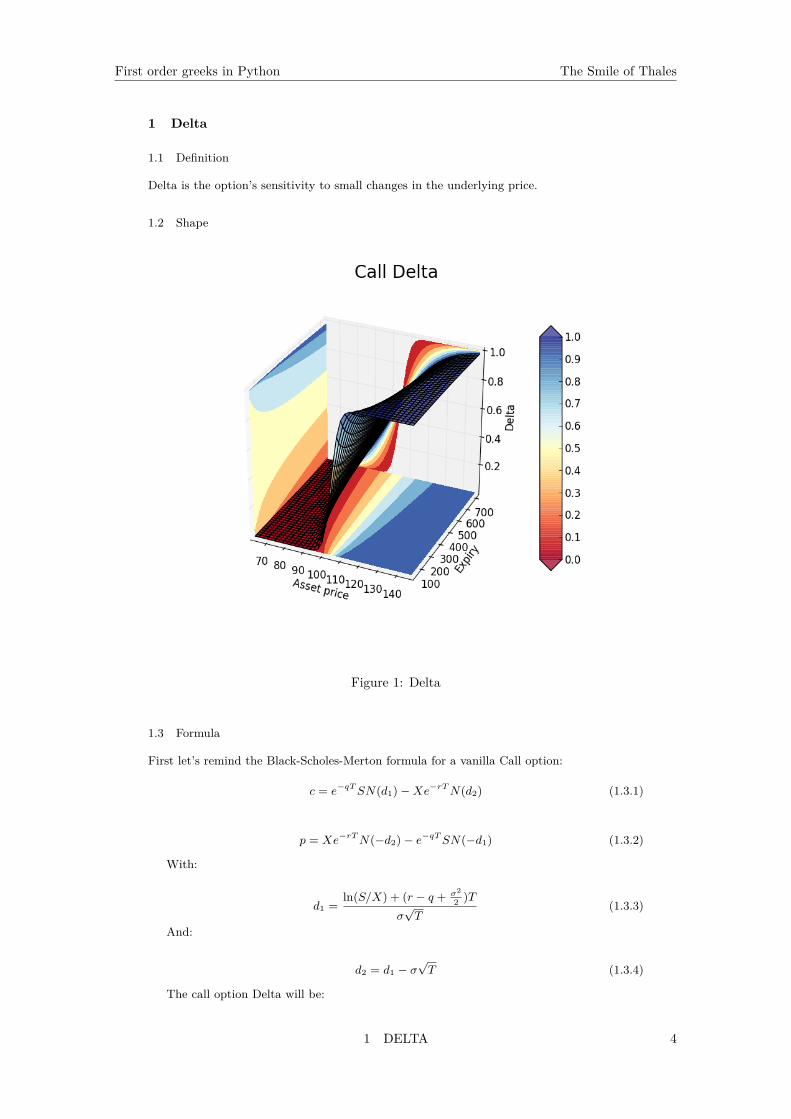
Delta is the option’s sensitivity to small changes in the underlying price.

1.2 Shape

Figure 1: Delta

1.3 Formula

First let’s remind the Black-Scholes-Merton formula for a vanilla Call option:

c = e−qTSN(d1)−Xe−rTN(d2) (1.3.1)

p = Xe−rTN(−d2)− e−qTSN(−d1) (1.3.2)

With:

d1 =ln(S/X) + (r − q + σ2

2 )Tσ√T

(1.3.3)

And:

d2 = d1 − σ√T (1.3.4)

The call option Delta will be:

1 DELTA 4


∆c = dc

dS= e−qTN(d1) (1.3.5)

1.4 Proof

∆c = dc

dS= d(e−qTSN(d1)−Xe−rTN(d2))

dS

=e−qTN(d1) + Se−qT∂N(d1)∂S

−Xe−rT ∂N(d2)∂S

=e−qTN(d1) + Se−qT∂d1

∂S

∂N(d1)∂d1

−Xe−rT ∂d2

∂S

∂N(d2)∂d2

=e−qTN(d1) + Se−qT∂d1

∂SN ′(d1)−Xe−rT ∂d2

∂SN ′(d2)

=e−qTN(d1) + Se−qTN ′(d1)Sσ√T

− Xe−rTN ′(d2)Sσ√T︸︷︷︸

I=0

(1.4.1)

Above, I=0. Indeed, according to (1.3.3) we have:

ln(S/X) + (r − q + σ2

2 )T = d1σ√T

⇒ ln(S)− ln(X) + (r − q)T = d1σ√T − σ2

2 T = 12[d2

1 − (d1 − σ√T )2]

⇒ ln(S) + ln( 1√2π

)− d21

2 = ln(X)− (r − q)T + ln( 1√2π

)− d22

2

⇒ S1√2πe−

d21

2 = Xe−(r−q)T 1√2πe−

d22

2

⇒ SN ′(d1) = Xe−(r−q)TN ′(d2)

⇒ Se−qTN ′(d1) = Xe−rTN ′(d2)

(1.4.2)

Finally from (1.4.1) we obtain:

∆c = e−qT N(d1) (1.4.3)

For the Put, since by parity we have:

p+ Se−qT = c+Xe−rT

⇒ dp

dS= dc

dS− e−qT

⇒∆p = N(d1) − 1

(1.4.4)

1.5 Python script

import numpy as npfrom math import sqrt , pi ,log , efrom enum import Enumimport scipy . stats as statfrom scipy . stats import normimport time

class BSMerton :def __init__ (self , args ):

self.Type = int(args [0]) # 1 for a Call , - 1 for a putself.S = float (args [1]) # Underlying asset priceself.K = float (args [2]) # Option strike Kself.r = float (args [3]) # Continuous risk fee rate

1 DELTA 5


self.q = float (args [4]) # Dividend continuous rateself.T = float (args [5]) / 365.0 # Compute time to expiryself. sigma = float (args [6]) # Underlying volatilityself. sigmaT = self. sigma * self.T ** 0.5# sigma *T for reusabilityself.d1 = (log(self.S / self.K) + \

(self.r - self.q + 0.5 * (self. sigma ** 2)) \* self.T) / self. sigmaT

self.d2 = self.d1 - self. sigmaT[self. Delta ] = self. delta ()

def delta (self ):dfq = e ** (-self.q * self.T)if self.Type == 1:

return [dfq * norm.cdf(self.d1 )]else:

return [dfq * (norm.cdf(self.d1) - 1)]

Now here is a piece of code that you can use to calculate and chart the Delta surfacedisplayed above (the python file that contains the Delta calculation above is called ”Option-sAnalytics.py”).

import numpy as npimport matplotlib . pyplot as pltfrom mpl_toolkits . mplot3d import Axes3Dimport mathfrom matplotlib import cmimport OptionsAnalyticsfrom OptionsAnalytics import BSMerton

# Option parameterssigma = 0.12 # Flat volatilitystrike = 105.0 # Fixed strikeepsilon = 0.4 # The % on the left/ right of Strike .

# Asset prices are centered around Spot (" ATM Spot ")shortexpiry = 30 # Shortest expiry in dayslongexpiry = 720 # Longest expiry in daysriskfree = 0.00 # Continuous risk free ratedivrate = 0.00 # Continuous div rate

# Grid definitiondx , dy = 40, 40 # Steps throughout asset price and expiries axis

# xx: Asset price axis , yy: expiry axis , zz: greek axisxx , yy = np. meshgrid (np. linspace ( strike *(1 - epsilon ), (1+ epsilon )* strike , dx), \

np. linspace ( shortexpiry , longexpiry , dy ))print " Calculating greeks ..."zz = np. array ([ BSMerton ([1 ,x,strike ,riskfree ,divrate ,y, sigma ]). Delta for

x,y in zip(np. ravel (xx), np. ravel (yy ))])zz = zz. reshape (xx. shape )

# Plot greek surfaceprint " Plotting surface ..."fig = plt. figure ()fig. suptitle (’Call Delta ’,fontsize =20)ax = fig.gca( projection =’3d’)surf = ax. plot_surface (xx , yy , zz , rstride =1, cstride =1, alpha =0.75 , cmap=cm. RdYlBu )ax. set_xlabel (’Asset price ’)ax. set_ylabel (’Expiry ’)ax. set_zlabel (’Delta ’)

# Plot 3D contourzzlevels = np. linspace (zz.min (),zz.max (), num =8, endpoint =True)xxlevels = np. linspace (xx.min (),xx.max (), num =8, endpoint =True)yylevels = np. linspace (yy.min (),yy.max (), num =8, endpoint =True)

1 DELTA 6


cset = ax. contourf (xx , yy , zz , zzlevels , zdir=’z’,offset =zz.min (),cmap=cm.RdYlBu , linestyles =’dashed ’)

cset = ax. contourf (xx , yy , zz , xxlevels , zdir=’x’,offset =xx.min (),cmap=cm.RdYlBu , linestyles =’dashed ’)

cset = ax. contourf (xx , yy , zz , yylevels , zdir=’y’,offset =yy.max (),cmap=cm.RdYlBu , linestyles =’dashed ’)

for c in cset. collections :c. set_dashes ([(0 , (2.0 , 2.0))]) # Dash contours

plt. clabel (cset , fontsize =10 , inline =1)

ax. set_xlim (xx.min (),xx.max ())ax. set_ylim (yy.min (),yy.max ())ax. set_zlim (zz.min (),zz.max ())

#ax. relim ()#ax. autoscale_view (True ,True ,True)

# Colorbarcolbar = plt. colorbar (surf , shrink =1.0 , extend =’both ’, aspect = 10)l,b,w,h = plt.gca (). get_position (). boundsll ,bb ,ww ,hh = colbar .ax. get_position (). boundscolbar .ax. set_position ([ll , b +0.1*h, ww , h *0.8])

# Show chartplt.show ()

1 DELTA 7


2 Gamma

2.1 Definition

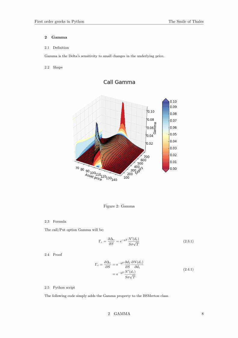
Gamma is the Delta’s sensitivity to small changes in the underlying price.

2.2 Shape

Figure 2: Gamma

2.3 Formula

The call/Put option Gamma will be:

Γc = ∂∆c

∂S= e−qT

N ′(d1)Sσ√T

(2.3.1)

2.4 Proof

Γc = ∂∆c

∂S= e−qT

∂d1

∂S

∂N(d1)∂d1

= e−qTN ′(d1)Sσ√T

(2.4.1)

2.5 Python script

The following code simply adds the Gamma property to the BSMerton class.

2 GAMMA 8



self.Type = int(args [0]) # 1 for a Call , - 1 for a putself.S = float (args [1]) # Underlying asset priceself.K = float (args [2]) # Option strike Kself.r = float (args [3]) # Continuous risk fee rateself.q = float (args [4]) # Dividend continuous rateself.T = float (args [5]) / 365.0 # Compute time to expiryself. sigma = float (args [6]) # Underlying volatilityself. sigmaT = self. sigma * self.T ** 0.5# sigma *T for reusabilityself.d1 = (log(self.S / self.K) + \


self.d2 = self.d1 - self. sigmaT[self. Delta ] = self. delta ()[self. Gamma ] = self. gamma ()

def gamma (self ):return [e ** (-self.q * self.T) * norm.pdf(self.d1) / (self.S * self. sigmaT )]

2 GAMMA 9


3 Vega

3.1 Definition

Vega is the option’s sensitivity to small changes in the underlying volatility.

3.2 Shape

Figure 3: Vega

3.3 Formula

The call/Put option Vega will be:

νc = νp = ∂c

∂σ= Se−qTN ′(d1)

√T (3.3.1)

3 VEGA 10


3.4 Proof

νc = ∂c

∂σ

= ∂(e−qTSN(d1)−Xe−rTN(d2))∂σ

= Se−qTN ′(d1)∂d1

∂σ−Xe−rTN ′(d2)∂d2

∂σ

= Se−qTN ′(d1)(√T − d1

σ)−Xe−rTN ′(d2)(∂d1

∂σ−√T )

= Se−qTN ′(d1)(√T − d1

σ)−Xe−rTN ′(d2)(−d1

σ)

= −d1

σ

[Se−qTN ′(d1)−Xe−rTN ′(d2)︸︷︷︸

I = 0

]+ Se−qTN ′(d1)

√T

= Se−qTN ′(d1)√T

(3.4.1)

3.5 Python script

The following code simply adds the Vega property to the BSMerton class.




self.d2 = self.d1 - self. sigmaT[self.Vega] = self.vega ()

# Vega for 1% change in voldef vega(self ):

return [0.01 * self.S * e ** (-self.q * self.T) * \norm.pdf(self.d1) * self.T ** 0.5]

3 VEGA 11


4 Theta

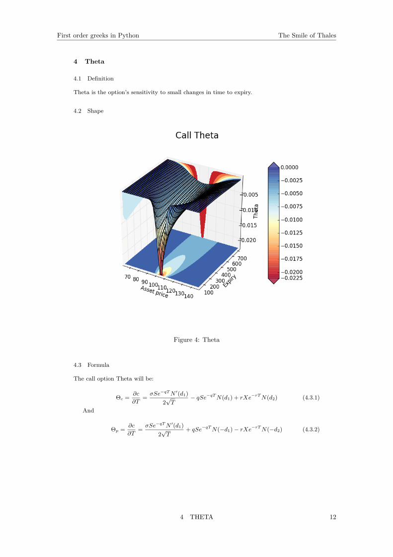
4.1 Definition

Theta is the option’s sensitivity to small changes in time to expiry.

4.2 Shape

Figure 4: Theta

4.3 Formula

The call option Theta will be:

Θc = ∂c

∂T= σSe−qTN ′(d1)

2√T

− qSe−qTN(d1) + rXe−rTN(d2) (4.3.1)

And

Θp = ∂c

∂T= σSe−qTN ′(d1)

2√T

+ qSe−qTN(−d1)− rXe−rTN(−d2) (4.3.2)

4 THETA 12


4.4 Proof

Θc = ∂c

∂T

= ∂(e−qTSN(d1)−Xe−rTN(d2))∂T

= − qSe−qTN(d1) + Se−qTN ′(d1)∂d1

∂T+ rXe−rTN(d2)−Xe−rTN ′(d2)∂d2

∂T

= rXe−rTN(d2)− qSe−qTN(d1) + Se−qTN ′(d1)∂d1

∂T−Xe−rTN ′(d2)∂(d1 − σ

√T )

∂T

= rXe−rTN(d2)− qSe−qTN(d1) + ∂d1

∂T

[Se−qTN ′(d1)−Xe−rTN ′(d2)]︸︷︷︸

=0,see(1.4.2)

+Xe−rTN ′(d2)σ2√T

= rXe−rTN(d2)− qSe−qTN(d1) + Se−qTN ′(d1)σ2√T

(4.4.1)

4.5 Python script

The following code simply adds the Theta property to the BSMerton class.




self.d2 = self.d1 - self. sigmaT[self. Theta ] = self. theta ()

# Theta for 1 day changedef theta (self ):

df = e ** -(self.r * self.T)dfq = e ** (-self.q * self.T)tmptheta = (1.0 / 365.0) \

* ( -0.5 * self.S * dfq * norm.pdf(self.d1) * \self. sigma / (self.T ** 0.5) + \

self.Type * (self.q * self.S * dfq * norm.cdf(self.Type * self.d1) \- self.r * self.K * df * norm.cdf(self.Type * self.d2 )))

return [ tmptheta ]

4 THETA 13


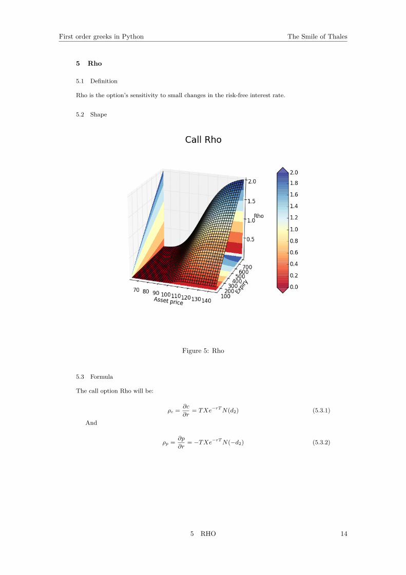
5 Rho

5.1 Definition

Rho is the option’s sensitivity to small changes in the risk-free interest rate.

5.2 Shape

Figure 5: Rho

5.3 Formula

The call option Rho will be:

ρc = ∂c

∂r= TXe−rTN(d2) (5.3.1)

And

ρp = ∂p

∂r= −TXe−rTN(−d2) (5.3.2)

5 RHO 14


5.4 Proof

ρc = ∂c

∂r

= ∂(e−qTSN(d1)−Xe−rTN(d2))∂r


∂r+ TXe−rTN(d2)−Xe−rTN ′(d2)∂d2

∂r


∂r+ TXe−rTN(d2)−Xe−rTN ′(d2)∂(d1 − σ

√T )

∂r

= ∂d1

∂r


=0,see(1.4.2)

] + Te−rTN(d2)

= Te−rTN(d2)

(5.4.1)

5.5 Python script

The following code simply adds the Rho property to the BSMerton class.




self.d2 = self.d1 - self. sigmaT[self.Rho] = self.rho ()

def rho(self ):df = e ** -(self.r * self.T)return [self.Type * self.K * self.T * df * 0.01 * norm.cdf(self.Type * self.d2 )]

5 RHO 15


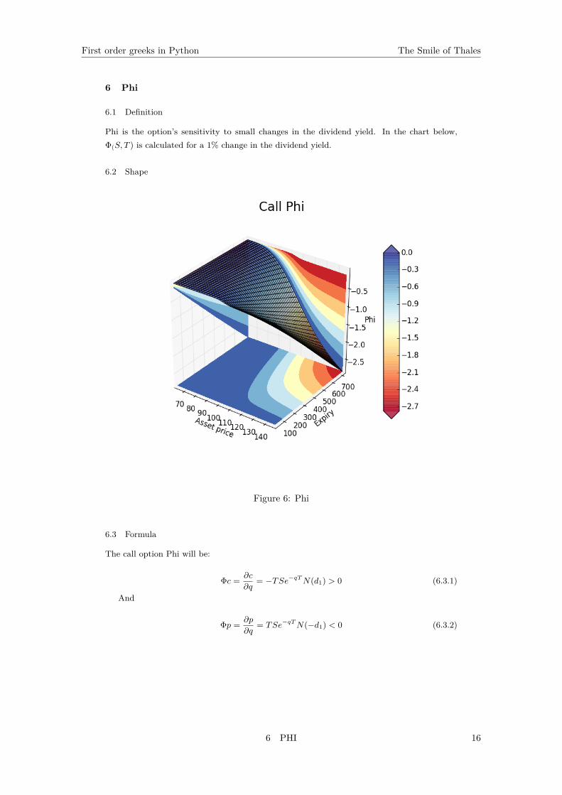
6 Phi

6.1 Definition

Phi is the option’s sensitivity to small changes in the dividend yield. In the chart below,Φ(S, T ) is calculated for a 1% change in the dividend yield.

6.2 Shape

Figure 6: Phi

6.3 Formula

The call option Phi will be:

Φc = ∂c

∂q= −TSe−qTN(d1) > 0 (6.3.1)

And

Φp = ∂p

∂q= TSe−qTN(−d1) < 0 (6.3.2)

6 PHI 16


6.4 Proof

Φc = ∂c

∂q

= ∂(e−qTSN(d1)−Xe−rTN(d2))∂q

= − TSe−qTN(d1) + Se−qTN(d1)∂d1

∂q−Xe−rTN ′(d2)∂d2

∂q

= ∂d1

∂q


=0,see(1.4.2)

]− TSe−qTN(d1)

= − TSe−qTN(d1)

(6.4.1)

6.5 Python script

The following code simply adds the Phi property to the BSMerton class.




self.d2 = self.d1 - self. sigmaT[self.Phi] = self.phi ()

def phi(self ):return [0.01* -self.Type * self.T * self.S * \

e ** (-self.q * self.T) * norm.cdf(self.Type * self.d1 )]

References

[1] Espen Gaarder Haug, The Complete Guide to Option Pricing Formulas. McGraw-Hill,2nd Edition, 2007.

REFERENCES 17

Documents

Greeks: option sensitivities, formula proofs and Python · Greeks: option sensitivities, formula proofs and Python scripts Part A - 1st order greeks The Smile of Thales April 11,